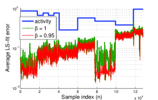
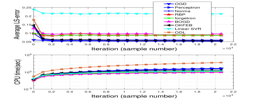
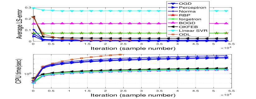
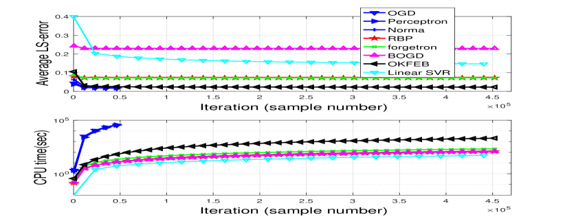
Large-scale Kernel-based Feature Extraction
via Low-rank Subspace Tracking on a Budget

Fatemeh Sheikholeslami,  Dimitris Berberidis,  and Georgios B. Giannakis Part of this work was presented in IEEE International Workshop on Computational Advances in Multi-Sensor Adaptive Processing (CAMSAP), Curacao, Dutch Antilles, Dec. 2017 [43].
This work was supported by NSF grants 1500713, 1514056, and the NIH grant no. 1R01GM104975-01. Preliminary parts of this work were presented at the Proc. of Globalsip Conf., Orlando, FL, Dec. 2015.
Authors are with the Dept. of Electrical and Comp. Engr. and the Digital Tech. Center, University of Minnesota, Minneapolis, MN 55455, USA.
E-mails: {sheik081,bermp001,georgios}@umn.edu
Abstract

Kernel-based methods enjoy powerful generalization capabilities in learning a variety of pattern recognition tasks. When such methods are provided with sufficient training data, broadly-applicable classes of nonlinear functions can be approximated with desired accuracy. Nevertheless, inherent to the nonparametric nature of kernel-based estimators are computational and memory requirements that become prohibitive with large-scale datasets. In response to this formidable challenge, the present work puts forward a low-rank, kernel-based, feature extraction approach that is particularly tailored for online operation. A novel generative model is introduced to approximate high-dimensional (possibly infinite) features via a low-rank nonlinear subspace, the learning of which lends itself to a kernel function approximation. Offline and online solvers are developed for the subspace learning task, along with affordable versions, in which the number of stored data vectors is confined to a predefined budget. Analytical results provide performance bounds on how well the kernel matrix as well as kernel-based classification and regression tasks can be approximated by leveraging budgeted online subspace learning and feature extraction schemes. Tests on synthetic and real datasets demonstrate and benchmark the efficiency of the proposed method for dynamic nonlinear subspace tracking as well as online classification and regressions tasks.

Index Terms:
Online nonlinear feature extraction, kernel methods, classification, regression, budgeted learning, nonlinear subspace tracking.

I Introduction

Kernel-based expansions can boost the generalization capability of learning tasks by powerfully modeling nonlinear functions, when linear functions fall short in practice. When provided with sufficient training data, kernel methods can approximate arbitrary nonlinear functions with desired accuracy. Although “data deluge” sets the stage by providing the “data-hungry” kernel methods with huge datasets, limited memory and computational constraints prevent such tools from fully exploiting their learning capabilities. In particular, given N𝑁N training D×1𝐷1D\times 1 vectors {𝐱ν}ν=1Nsuperscriptsubscriptsubscript𝐱𝜈𝜈1𝑁\{{\bf x}_{\nu}\}_{\nu=1}^{N}, kernel regression or classification machines take 𝒪(N2D)𝒪superscript𝑁2𝐷\mathcal{O}(N^{2}D) operations to form the N×N𝑁𝑁N\times N kernel matrix 𝐊𝐊{\bf K}, memory 𝒪(N2)𝒪superscript𝑁2\mathcal{O}(N^{2}) to store it, and 𝒪(N3)𝒪superscript𝑁3\mathcal{O}(N^{3}) computational complexity to find the sought predictor or classifier.

In this context, several efforts have been made in different fields of stochastic optimization, functional analysis, and numerical linear algebra to speed up kernel machines for “big data” applications [21, 9, 41, 12, 52, 33, 26]. A common approach to scaling up kernel methods is to approximate the kernel matrix 𝐊𝐊{\bf K} by a low-rank factorization; that is, 𝐊𝐊^:=𝐙𝐙similar-to-or-equals𝐊^𝐊assignsuperscript𝐙top𝐙{\bf K}\simeq\hat{{\bf K}}:={\bf Z}^{\top}{\bf Z}, where 𝐙r×N𝐙superscript𝑟𝑁{\bf Z}\in\mathbb{R}^{r\times N} with r(N)annotated𝑟much-less-thanabsent𝑁r\;(\ll N) is the reduced rank, through which storage and computational requirements go down to 𝒪(Nr)𝒪𝑁𝑟\mathcal{O}(Nr) and 𝒪(Nr2)𝒪𝑁superscript𝑟2\mathcal{O}(Nr^{2}), respectively. Kernel (K)PCA [38] provides a viable factorization for a such low-rank approximation, at the cost of order 𝒪(N2r)𝒪superscript𝑁2𝑟\mathcal{O}(N^{2}r) computations. Alternatively, a low-rank factorization can be effected by randomly selecting r𝑟r training vectors to approximate the kernel matrix [23]. Along these lines, Nystrom approximation [52], and its advanced renditions [12, 54, 22, 44, 48] are popular among this class of randomized factorizations. They trade off accuracy in approximating 𝐊𝐊{\bf K} with 𝐊^^𝐊\hat{{\bf K}}, for reducing KPCA complexity from 𝒪(N2r)𝒪superscript𝑁2𝑟\mathcal{O}(N^{2}r) to 𝒪(Nr)𝒪𝑁𝑟\mathcal{O}(Nr). Their merits are well-documented for nonlinear regression and classification tasks performed offline [8, 55, 1]. Rather than factorizing 𝐊𝐊{\bf K}, one can start from high-dimensional (lifted) feature vectors ϕ(𝐱ν)bold-italic-ϕsubscript𝐱𝜈\bm{\phi}({\bf x}_{\nu}) whose inner product induces the kernel κ(𝐱i,𝐱j):=ϕ(𝐱i),ϕ(𝐱j)assign𝜅subscript𝐱𝑖subscript𝐱𝑗bold-italic-ϕsubscript𝐱𝑖bold-italic-ϕsubscript𝐱𝑗\kappa({\bf x}_{i},{\bf x}_{j}):=\langle{\bm{\phi}}({\bf x}_{i}),{\bm{\phi}}({\bf x}_{j})\rangle [33, 53, 25, 26, 42]. Approximating ϕ(𝐱)bold-italic-ϕ𝐱{\bm{\phi}}({\bf x}) through an r×1𝑟1r\times 1 vector 𝐳𝐳{\bf z}, the nonlinear kernel can be approximated by a linear one as κ(𝐱i,𝐱j)𝐳i𝐳jsimilar-to-or-equals𝜅subscript𝐱𝑖subscript𝐱𝑗superscriptsubscript𝐳𝑖topsubscript𝐳𝑗\kappa({\bf x}_{i},{\bf x}_{j})\simeq{\bf z}_{i}^{\top}{\bf z}_{j}. Exploiting the fast linear learning machines [13, 41], the kernel-based task then reduces to learning a linear function over features {𝐳ν}ν=1Nsuperscriptsubscriptsubscript𝐳𝜈𝜈1𝑁\{{\bf z}_{\nu}\}_{\nu=1}^{N}, which can be achieved in 𝒪(Nr)𝒪𝑁𝑟\mathcal{O}(Nr) operations. Such a computationally attractive attribute is common to both kernel matrix factorization and lifted feature approximation. Note however, that online Nystrom-type schemes are not available, while feature approximation algorithms are randomized, and thus they are not data driven.

Different from kernel matrix and feature approximations performed in batch form, online kernel-based learning algorithms are of paramount importance. Instead of loading the entire datasets in memory, online methods iteratively pass over the set from an external memory [21, 41, 45, 5, 18, 40, 20]. This is also critical when the entire dataset is not available beforehand, but is acquired one datum at a time. For large data streams however, as the number of data increases with time, the support vectors (SVs) through which the function is estimated, namely the set 𝒮𝒮\mathcal{S} in the approximation f(𝐱)f^(𝐱)=i𝒮αiκ(𝐱i,𝐱)similar-to-or-equals𝑓𝐱^𝑓𝐱subscript𝑖𝒮subscript𝛼𝑖𝜅subscript𝐱𝑖𝐱f({\bf x})\simeq\hat{f}({\bf x})=\sum_{i\in\mathcal{S}}\alpha_{i}\kappa({\bf x}_{i},{\bf x}), also increases in size. Thus, the function evaluation delay as well as the required memory for storing the SV set eventually become unaffordable. Efforts have been devoted to reducing the number of SVs while trying to maintain performance on unseen data (a.k.a. generalization capability) [11]. In more recent attempts, by restricting the maximum number of SVs to a predefined budget B𝐵B, the growth of algorithmic complexity is confined to an affordable limit, that is maintained throughout the online classification [50, 49, 10] or regression [47] task.

The present work builds a generative model according to which the high (possibly infinite)-dimensional features are approximated by their projection onto a low-rank subspace, thus providing a linear kernel function approximation (Section II). In contrast to [33, 12, 54, 25], where due to the nature of randomization the number of required features for providing an accurate kernel function approximation is often large, systematically learning the ambient nonlinear subspace yields an accurate approximation through a smaller number of extracted features.

Offline and online solvers for subspace learning are developed, and their convergence is analyzed in Sections III and IV respectively. In order to keep the complexity and memory requirements affordable, budgeted versions of the proposed algorithms are devised in Section V, in which the number of stored data vectors is confined to a predefined budget B𝐵B. Budget maintenance is performed through a greedy approach, whose effectiveness is corroborated through simulated tests. This is the first work to address dynamic nonlinear (kernel-based) feature extraction under limited memory resources.

Analytical results in Section VI provide performance bounds on how well the kernel matrix as well as kernel-based classification and regression can be approximated by leveraging the novel budgeted online subspace-learning and feature-extraction approach. Finally, Section VII presents experiments on synthetic and real datasets, demonstrating the efficiency of the proposed methods in terms of accuracy and run time.

II Preliminaries and Problem Statement

Consider N𝑁N real data vectors {𝐱ν}ν=1Nsuperscriptsubscriptsubscript𝐱𝜈𝜈1𝑁\{{\bf x}_{\nu}\}_{\nu=1}^{N} of size D×1𝐷1D\times 1. As large values of D𝐷D and N𝑁N hinder storage and processing of such datasets, extracting informative features from the data (a.k.a. dimensionality reduction) results in huge savings on memory and computational requirements. This fundamentally builds on the premise that the informative part of the data is of low dimension r<D𝑟𝐷r<D, and thus the data {𝐱ν}ν=1Nsuperscriptsubscriptsubscript𝐱𝜈𝜈1𝑁\{{\bf x}_{\nu}\}_{\nu=1}^{N} are well represented by the generative model

𝐱ν=𝐋𝐪ν+𝐯ν,ν=1,,Nformulae-sequencesubscript𝐱𝜈subscript𝐋𝐪𝜈subscript𝐯𝜈𝜈1𝑁{\bf x}_{\nu}={\bf L}{\bf q}_{\nu}+\mathbf{v}_{\nu}\;,\quad\nu=1,\ldots,N (1)

where the tall D×r𝐷𝑟D\times r matrix 𝐋𝐋{\bf L} has rank r<D𝑟𝐷r<D; vector 𝐪νsubscript𝐪𝜈{\bf q}_{\nu} is the r×1𝑟1r\times 1 projection of 𝐱νsubscript𝐱𝜈{\bf x}_{\nu} onto the column space of 𝐋𝐋{\bf L}; and 𝐯νsubscript𝐯𝜈\mathbf{v}_{\nu} denotes zero-mean additive noise.

Pursuit of the subspace 𝐋𝐋{\bf L} and the low-dimensional features {𝐪ν}ν=1Nsuperscriptsubscriptsubscript𝐪𝜈𝜈1𝑁\{{\bf q}_{\nu}\}_{\nu=1}^{N} is possible using a blind least-squares (LS) criterion regularized by a rank-promoting term using e.g., the nuclear norm of 𝐗^=𝐋𝐐N^𝐗subscript𝐋𝐐𝑁\hat{\mathbf{X}}={\bf L}{\bf Q}_{N}, where 𝐐N:=[𝐪1,,𝐪N]assignsubscript𝐐𝑁subscript𝐪1subscript𝐪𝑁{\bf Q}_{N}:=[{\bf q}_{1},...,{\bf q}_{N}] [35]. Albeit convex, nuclear-norm regularization is not attractive for sequential learning.

To facilitate reducing the computational complexity, it is henceforth assumed that an upper bound on the rank of matrix 𝐗^^𝐗\hat{{\bf X}} is given ρrank(𝐗^)𝜌rank^𝐗\rho\geq\text{rank}(\hat{{\bf X}}). 111In practice, the rank is controlled by tuning regularization parameter, as it can be made small enough for sufficiently large λ𝜆\lambda. Thus, building on the work of [29] by selecting rρ𝑟𝜌r\geq\rho, and to arrive at a scalable subspace tracker, here we surrogate the nuclear norm with the summation of the Frobenious-norms of 𝐋𝐋{\bf L} and 𝐐Nsubscript𝐐𝑁{\bf Q}_{N}, which yields (cf. Prop. 1 in [29] for proof on equivalence)

min𝐋,{𝐪ν}ν=1N12Nν=1n𝐱ν𝐋𝐪ν22+λ2N(𝐋F2+𝐐NF2)subscript𝐋superscriptsubscriptsubscript𝐪𝜈𝜈1𝑁12𝑁superscriptsubscript𝜈1𝑛superscriptsubscriptnormsubscript𝐱𝜈subscript𝐋𝐪𝜈22𝜆2𝑁superscriptsubscriptnorm𝐋𝐹2superscriptsubscriptnormsubscript𝐐𝑁𝐹2\min_{{\bf L},\{{\bf q}_{\nu}\}_{\nu=1}^{N}}{\dfrac{1}{2N}\sum_{\nu=1}^{n}{\|{\bf x}_{\nu}-{\bf L}{\bf q}_{\nu}\|_{2}^{2}}+\dfrac{\lambda}{2N}\Big{(}\|{\bf L}\|_{F}^{2}+\|{\bf Q}_{N}\|_{F}^{2}\Big{)}} (2)

where λ𝜆\lambda controls the tradeoff between LS fit and rank regularization [28]. Principal component analysis (PCA) - the “workhorse” of dimensionality reduction- solves (2) when the rank regularization is replaced with orthonormality constraints on 𝐋𝐋{\bf L}. Undoubtedly, the accuracy of any linear dimensionality reduction method is dictated by how well the model (1) fits a given dataset, which is related to how well the corresponding data covariance matrix can be approximated by a low-rank matrix [17, p. 534].

In practice however, low-rank linear models often fail to accurately capture the datasets. A means to deal with nonlinearities in pattern recognition tasks, is to first map vectors {𝐱ν}ν=1Nsuperscriptsubscriptsubscript𝐱𝜈𝜈1𝑁\{{\bf x}_{\nu}\}_{\nu=1}^{N} to a higher D¯¯𝐷\bar{D}-dimensional space using a function ϕ:DD¯:bold-italic-ϕsuperscript𝐷superscript¯𝐷\bm{\phi}:\mathbb{R}^{D}\rightarrow\mathbb{R}^{\bar{D}} (possibly with D¯=¯𝐷{\bar{D}}=\infty), and subsequently seek a linear function over the lifted data ϕ(𝐱)bold-italic-ϕ𝐱\bm{\phi}({\bf x}). This map induces a so-termed kernel function κ(𝐱i,𝐱j)=ϕ(𝐱i)ϕ(𝐱j)𝜅subscript𝐱𝑖subscript𝐱𝑗superscriptbold-italic-ϕtopsubscript𝐱𝑖bold-italic-ϕsubscript𝐱𝑗\kappa({\bf x}_{i},{\bf x}_{j})=\bm{\phi}^{\top}({\bf x}_{i})\bm{\phi}({\bf x}_{j}). Selecting the kernel to have a closed-form expression circumvents the need to explicitly know {ϕ(𝐱ν)}ν=1Nsuperscriptsubscriptbold-italic-ϕsubscript𝐱𝜈𝜈1𝑁\{\bm{\phi}({\bf x}_{\nu})\}_{\nu=1}^{N} - what is referred to as the “kernel trick.” Similarly, the norm corresponding to the reproducing kernel Hilbert space (RKHS) is defined as ϕ(𝐱)2:=ϕ(𝐱),ϕ(𝐱)=κ(𝐱,𝐱)assignsuperscriptsubscriptnormitalic-ϕ𝐱2bold-italic-ϕ𝐱bold-italic-ϕ𝐱𝜅𝐱𝐱\|\mathbf{\phi}(\mathbf{x})\|_{\mathcal{H}}^{2}:=\langle\bm{\phi}({\bf x}),\bm{\phi}({\bf x})\rangle=\kappa({\bf x},{\bf x}). Upon defining the D¯×N¯𝐷𝑁\bar{D}\times N matrix 𝚽N:=[ϕ(𝐱1),,ϕ(𝐱N)]assignsubscript𝚽𝑁bold-italic-ϕsubscript𝐱1bold-italic-ϕsubscript𝐱𝑁\bm{\Phi}_{N}:=[\bm{\phi}({\bf x}_{1}),...,\bm{\phi}({\bf x}_{N})], the N×N𝑁𝑁N\times N kernel matrix related to the covariance of the lifted data is formed with (i,j)𝑖𝑗(i,j) entry κ(𝐱i,𝐱j)𝜅subscript𝐱𝑖subscript𝐱𝑗\kappa({\bf x}_{i},{\bf x}_{j}) as 𝐊(𝐱1:N,𝐱1:N)=𝚽N𝚽N𝐊subscript𝐱:1𝑁subscript𝐱:1𝑁superscriptsubscript𝚽𝑁topsubscript𝚽𝑁{\bf K}({\bf x}_{1:N},{\bf x}_{1:N})=\bm{\Phi}_{N}^{\top}\bm{\Phi}_{N}, where 𝐱1:N:=vec[𝐱1,𝐱2,,𝐱N]assignsubscript𝐱:1𝑁vecsubscript𝐱1subscript𝐱2subscript𝐱𝑁{\bf x}_{1:N}:=\text{vec}[{\bf x}_{1},{\bf x}_{2},...,{\bf x}_{N}]. Its computation and storage incurs complexity 𝒪(N2D)𝒪superscript𝑁2𝐷\mathcal{O}(N^{2}D) and 𝒪(N2)𝒪superscript𝑁2\mathcal{O}(N^{2}) respectively, which is often not affordable when Nmuch-greater-than𝑁absentN\gg and/or Dmuch-greater-than𝐷absentD\gg.

Fortunately, 𝐊𝐊{\bf K} for large data sets in practice has approximately low rank. This fact is exploited in e.g., [53, 12] and [52] to approximate 𝐊𝐊{\bf K} via a low-rank factorization, hence reducing the evaluation and memory requirements of offline kernel-based learning tasks from 𝒪(N2)𝒪superscript𝑁2\mathcal{O}(N^{2}) down to 𝒪(Nr)𝒪𝑁𝑟\mathcal{O}(Nr). Here, we further build on this observation to deduce that the low-rank property of 𝐊=𝚽N𝚽N𝐊subscriptsuperscript𝚽top𝑁subscript𝚽𝑁{\bf K}=\bm{\Phi}^{\top}_{N}\bm{\Phi}_{N} implies that 𝚽Nsubscript𝚽𝑁\bm{\Phi}_{N} can also be approximated by a low-rank matrix, thus motivating our pursuit of online low-rank factorization of 𝚽Nsubscript𝚽𝑁\bm{\Phi}_{N}. To this end, instead of projecting {𝐱ν}subscript𝐱𝜈\{{\bf x}_{\nu}\}s onto the columns of 𝐋𝐋{\bf L} as in (2), we will project {ϕ(𝐱ν)}bold-italic-ϕsubscript𝐱𝜈\{\bm{\phi}({\bf x}_{\nu})\}s on 𝐋¯D¯×r¯𝐋superscript¯𝐷𝑟\bar{{\bf L}}\in\mathbb{R}^{\bar{D}\times r}, whose columns span what we refer to as “virtual” column subspace since D¯¯𝐷\bar{D} can be infinite. Specifically, we consider [cf. (2)]

min𝐋¯,{𝐪ν}ν=1N12Nν=1Nϕ(𝐱ν)𝐋¯𝐪ν2+λ2N(𝐋¯HS2+𝐐NF2)subscript¯𝐋superscriptsubscriptsubscript𝐪𝜈𝜈1𝑁12𝑁superscriptsubscript𝜈1𝑁superscriptsubscriptnormbold-italic-ϕsubscript𝐱𝜈¯𝐋subscript𝐪𝜈2𝜆2𝑁superscriptsubscriptnorm¯𝐋𝐻𝑆2superscriptsubscriptnormsubscript𝐐𝑁𝐹2\min_{{\bar{{\bf L}},\{{\bf q}_{\nu}\}_{\nu=1}^{N}}}\dfrac{1}{2N}\sum_{\nu=1}^{N}{\|\bm{\phi}({\bf x}_{\nu})-\bar{{\bf L}}{\bf q}_{\nu}\|_{\mathcal{H}}^{2}}+\dfrac{\lambda}{2N}\Big{(}\|\bar{{\bf L}}\|_{HS}^{2}+\|{\bf Q}_{N}\|_{F}^{2}\Big{)} (3)

where the 2subscript2\ell_{2}-norm has been substituted by the \mathcal{H}-norm in the D¯¯𝐷\bar{D}-dimensional Hilbert space. Similarly, let the Hilbert–Schmidt operator be defined as 𝐋¯HS=Tr(𝐋¯𝐋¯):=c=1r𝐥¯c2subscriptnorm¯𝐋𝐻𝑆Trsuperscript¯𝐋top¯𝐋assignsuperscriptsubscript𝑐1𝑟superscriptsubscriptnormsubscript¯𝐥𝑐2\|\bar{{\bf L}}\|_{HS}=\sqrt{\text{Tr}(\bar{{\bf L}}^{\top}\bar{{\bf L}})}:={\sqrt{\sum_{c=1}^{r}\|\bar{\mathbf{l}}_{c}\|_{\mathcal{H}}^{2}}} with 𝐥¯csubscript¯𝐥𝑐\bar{\mathbf{l}}_{c} denoting the c𝑐c-th column of 𝐋¯¯𝐋\bar{{\bf L}}. Note that for Euclidean spaces, the Hilbert-Schmidt norm reduces to the Frobenious norm.

Observe also that similar to the linear model in (2), upon removing the regularization terms and adding the orthonormality constraints on the columns of 𝐋¯¯𝐋\bar{{\bf L}}, (3) reduces to that of KPCA (without centering) in primal domain [38, p. 429]. The present formulation in (3) however, enables us to develop sequential learning algorithms, which will later be enhanced with a tracking capability for dynamic datasets.

For a fixed 𝐐Nsubscript𝐐𝑁{\bf Q}_{N}, the criterion in (3) is minimized by

𝐋¯N=𝚽N𝐐N(𝐐N𝐐N+λ𝐈)1:=𝚽N𝐀subscript¯𝐋𝑁subscript𝚽𝑁superscriptsubscript𝐐𝑁topsuperscriptsubscript𝐐𝑁superscriptsubscript𝐐𝑁top𝜆𝐈1assignsubscript𝚽𝑁𝐀{\bar{\bf L}}_{N}=\bm{\Phi}_{N}{\bf Q}_{N}^{\top}\Big{(}{\bf Q}_{N}{\bf Q}_{N}^{\top}+{\lambda}\mathbf{I}\Big{)}^{-1}:=\bm{\Phi}_{N}{\bf A}\; (4)

where the N×r𝑁𝑟N\times r factor 𝐀𝐀{\bf A} can be viewed as “morphing’ the columns of 𝚽Nsubscript𝚽𝑁\bm{\Phi}_{N} to offer a flexible basis for the lifted data. Substituting (4) back into (3) and exploiting the kernel trick, we arrive at

min𝐀,{𝐪ν}ν=1Nsubscript𝐀superscriptsubscriptsubscript𝐪𝜈𝜈1𝑁\displaystyle\min_{{\bf A},\{{\bf q}_{\nu}\}_{\nu=1}^{N}} 12Nν=1N(κ(𝐱ν,𝐱ν)2𝐤(𝐱1:N,𝐱ν)𝐀𝐪ν\displaystyle\quad\dfrac{1}{2N}\sum_{\nu=1}^{N}\Big{(}\kappa({\bf x}_{\nu},{\bf x}_{\nu})-2{\bf k}^{\top}({\bf x}_{1:N},{\bf x}_{\nu}){\bf A}{\bf q}_{\nu} (5)
+𝐪ν𝐀𝐊(𝐱1:N,𝐱1:N)𝐀𝐪ν)\displaystyle\qquad\qquad+{\bf q}_{\nu}^{\top}{\bf A}^{\top}{\bf K}({\bf x}_{1:N},{\bf x}_{1:N}){\bf A}{\bf q}_{\nu}\Big{)}
+λ2N(tr{𝐀𝐊(𝐱1:N,𝐱1:N)𝐀}+ν=1N𝐪ν22)𝜆2𝑁trsuperscript𝐀top𝐊subscript𝐱:1𝑁subscript𝐱:1𝑁𝐀superscriptsubscript𝜈1𝑁superscriptsubscriptnormsubscript𝐪𝜈22\displaystyle+\dfrac{\lambda}{2N}\Big{(}\text{tr}\{{\bf A}^{\top}\mathbf{K}({\bf x}_{1:N},{\bf x}_{1:N}){\bf A}\}+\sum_{\nu=1}^{N}\|{\bf q}_{\nu}\|_{2}^{2}\Big{)}

where the N×1𝑁1N\times 1 vector 𝐤(𝐱1:N,𝐱n)𝐤subscript𝐱:1𝑁subscript𝐱𝑛{\bf k}({\bf x}_{1:N},{\bf x}_{n}) in (5) is the n𝑛n-th column of 𝐊(𝐱1:N,𝐱1:N)𝐊subscript𝐱:1𝑁subscript𝐱:1𝑁{\bf K}({\bf x}_{1:N},{\bf x}_{1:N}), and since 𝐀𝐀{\bf A} has size N×r𝑁𝑟N\times r, the minimization in (5) does not depend on D¯¯𝐷\bar{D}.

Our goal is to develop and analyze batch as well as online solvers for (5). By pre-specifying an affordable complexity for the online solver, we aim at a low-complexity algorithm where subspace learning and feature extraction can be performed on-the-fly for streaming applications. Furthermore, we will introduce a novel approach to extracting features on which the kernel-based learning tasks of complexity 𝒪(N3)𝒪superscript𝑁3\mathcal{O}(N^{3}) can be well approximated by linear counterparts of complexity 𝒪(rN)𝒪𝑟𝑁\mathcal{O}(rN), hence realizing great savings in memory and computation while maintaining performance. A remark is now in order.

Remark 1. The subspace 𝐋¯Nsubscript¯𝐋𝑁\bar{{\bf L}}_{N} in (4) can be thought as a dictionary whose atoms are morphed via factor 𝐀𝐀{\bf A}. Sparse representation over kernel-based dictionaries have been considered [37, 16, 46, 30]. Different from these approaches however, the novelty here is on developing algorithms that can process streaming datasets, possibly with dynamic underlying generative models. Thus, our goal is to efficiently learn and track a dictionary that adequately captures streaming data vectors, and can afford a low-rank approximation of the underlying high-dimensional map.

III Offline kernel based Feature Extraction

Given a dataset {𝐱ν}ν=1Nsuperscriptsubscriptsubscript𝐱𝜈𝜈1𝑁\{{\bf x}_{\nu}\}_{\nu=1}^{N} and leveraging the bi-convexity of the minimization in (5), we introduce in this section a batch solver, where two blocks of variables (𝐀𝐀{\bf A} and {𝐪ν}ν=1Nsuperscriptsubscriptsubscript𝐪𝜈𝜈1𝑁\{{\bf q}_{\nu}\}_{\nu=1}^{N}) are updated alternately. The following two updates are carried out iteratively until convergence.

Update 1. With 𝐀[k]𝐀delimited-[]𝑘{\bf A}[k] given from iteration k𝑘k, the projection vectors {𝐪ν}ν=1Nsuperscriptsubscriptsubscript𝐪𝜈𝜈1𝑁\{{\bf q}_{\nu}\}_{\nu=1}^{N} in iteration k+1𝑘1k+1 are updated as

𝐪ν[k+1]=argmin𝐪subscript𝐪𝜈delimited-[]𝑘1subscript𝐪\displaystyle{\bf q}_{\nu}[k+1]=\arg\min_{{\bf q}}\quad (𝐱ν;𝐀[k],𝐪;𝐱1:N)+λ2𝐪22subscript𝐱𝜈𝐀delimited-[]𝑘𝐪subscript𝐱:1𝑁𝜆2superscriptsubscriptnorm𝐪22\displaystyle\ell({\bf x}_{\nu};{\bf A}[k],{\bf q};{\bf x}_{1:N})+\dfrac{\lambda}{2}\|{\bf q}\|_{2}^{2} (6a)
where the fitting cost (.)\ell(.) is given by [cf. (3)-(5)]
(𝐱ν;𝐀[k],𝐪;𝐱1:N)subscript𝐱𝜈𝐀delimited-[]𝑘𝐪subscript𝐱:1𝑁\displaystyle\ell({\bf x}_{\nu};{\bf A}[k],{\bf q};{\bf x}_{1:N}) :=12ϕ(𝐱ν)𝚽N𝐀[k]𝐪2assignabsent12superscriptsubscriptnormbold-italic-ϕsubscript𝐱𝜈subscript𝚽𝑁𝐀delimited-[]𝑘𝐪2\displaystyle:=\dfrac{1}{2}\|{\bm{\phi}}({\bf x}_{\nu})-{\bm{\Phi}}_{N}{\bf A}[k]{\bf q}\|_{\mathcal{H}}^{2} (6b)
=κ(𝐱ν,𝐱ν)2𝐤(𝐱1:N,𝐱ν)𝐀[k]𝐪absent𝜅subscript𝐱𝜈subscript𝐱𝜈2superscript𝐤topsubscript𝐱:1𝑁subscript𝐱𝜈𝐀delimited-[]𝑘𝐪\displaystyle\;=\kappa({\bf x}_{\nu},{\bf x}_{\nu})-2{\bf k}^{\top}({\bf x}_{1:N},{\bf x}_{\nu}){\bf A}[k]{\bf q}
+𝐪𝐀[k]𝐊(𝐱1:N,𝐱1:N)𝐀[k]𝐪.superscript𝐪topsuperscript𝐀topdelimited-[]𝑘𝐊subscript𝐱:1𝑁subscript𝐱:1𝑁𝐀delimited-[]𝑘𝐪\displaystyle\,\quad+{\bf q}^{\top}{\bf A}^{\top}[k]{\bf K}({\bf x}_{1:N},{\bf x}_{1:N}){\bf A}[k]{\bf q}\;.

The minimizer of (6a) yields the features as regularized projection coefficients of the lifted data vectors onto the virtual subspace 𝐋¯N[k]=𝚽N𝐀[k]subscript¯𝐋𝑁delimited-[]𝑘subscript𝚽𝑁𝐀delimited-[]𝑘\bar{{\bf L}}_{N}[k]=\bm{\Phi}_{N}{\bf A}[k], and is given in closed form by

𝐪ν[k+1]subscript𝐪𝜈delimited-[]𝑘1\displaystyle{\bf q}_{\nu}[k+1] =(𝐀[k]𝐊(𝐱1:N,𝐱1:N)𝐀[k]+λ𝐈r)1absentsuperscriptsuperscript𝐀topdelimited-[]𝑘𝐊subscript𝐱:1𝑁subscript𝐱:1𝑁𝐀delimited-[]𝑘𝜆subscript𝐈𝑟1\displaystyle=({\bf A}^{\top}[k]\mathbf{K}({\bf x}_{1:N},{\bf x}_{1:N}){\bf A}[k]+\lambda\mathbf{I}_{r})^{-1}
×𝐀[k]𝐤(𝐱1:N,𝐱ν),ν=1,,N.\displaystyle\;\times{\bf A}^{\top}[k]{\bf k}({\bf x}_{1:N},{\bf x}_{\nu}),\quad\nu=1,...,N\;. (7)

Update 2. With {𝐪ν[k+1]}ν=1Nsuperscriptsubscriptsubscript𝐪𝜈delimited-[]𝑘1𝜈1𝑁\{{\bf q}_{\nu}[k+1]\}_{\nu=1}^{N} fixed and after dropping irrelevant terms, the subspace factor is obtained as [cf. (5)]

𝐀[k+1]=argmin𝐀𝐀delimited-[]𝑘1subscript𝐀\displaystyle{\bf A}[k+1]=\arg\min_{\bf A} 1Nν=1N(𝐱ν;𝐀,𝐪ν[k+1];𝐱1:N)1𝑁superscriptsubscript𝜈1𝑁subscript𝐱𝜈𝐀subscript𝐪𝜈delimited-[]𝑘1subscript𝐱:1𝑁\displaystyle\dfrac{1}{N}\sum_{\nu=1}^{N}\ell({\bf x}_{\nu};{\bf A},{\bf q}_{\nu}[k+1];{\bf x}_{1:N})
+λ2Ntr{𝐀𝐊(𝐱1:N,𝐱1:N)𝐀}.𝜆2𝑁trsuperscript𝐀top𝐊subscript𝐱:1𝑁subscript𝐱:1𝑁𝐀\displaystyle+\dfrac{\lambda}{2N}\text{tr}\{{\bf A}^{\top}\mathbf{K}({\bf x}_{1:N},{\bf x}_{1:N}){\bf A}\}\;. (8)

Since 𝐊𝐊{\bf K} is positive definite in practice, (III) involves a strictly convex minimization. Equating the gradient to zero, yields the wanted subspace factor in closed form

𝐀[k+1]=𝐐N[k+1](𝐐N[k+1]𝐐N[k+1]+λ𝐈r)1.𝐀delimited-[]𝑘1superscriptsubscript𝐐𝑁topdelimited-[]𝑘1superscriptsubscript𝐐𝑁delimited-[]𝑘1superscriptsubscript𝐐𝑁topdelimited-[]𝑘1𝜆subscript𝐈𝑟1{\bf A}[k+1]={\bf Q}_{N}^{\top}[k+1]\Big{(}{\bf Q}_{N}[k+1]{\bf Q}_{N}^{\top}[k+1]+{\lambda}\mathbf{I}_{r}\Big{)}^{-1}\;. (9)

Algorithm 1 provides the pseudocode for the update rules (III) and (9) of the batch solver, and the following proposition gives a guarantee on the convergence of the proposed solver to a local stationary point.

Proposition 1. For positive definite kernels and λ>0𝜆0\lambda>0, the sequence {𝐀[k],𝐐N[k]}𝐀delimited-[]𝑘subscript𝐐𝑁delimited-[]𝑘\{{\bf A}[k],{\bf Q}_{N}[k]\} generated by Algorithm 1 converges to a stationary point of the minimization in (5).

Proof: Since the minimizations in (6a) and (III) are strictly convex with unique solutions, the result follows readily from [3, p. 272]. \hfill\blacksquare

Algorithm 1 BKFE: Batch Kernel-based Feature Extraction
Input {𝐱ν}ν=1N,λsuperscriptsubscriptsubscript𝐱𝜈𝜈1𝑁𝜆\{{\bf x}_{\nu}\}_{\nu=1}^{N},\lambda
Initialize 𝐀[1]𝐀delimited-[]1{\bf A}{[1]} at random
For k=1,𝑘1k=1,\ldots do
𝐒[k+1]=(𝐀[k]𝐊(𝐱1:N,𝐱1:N)𝐀[k]+λ𝐈r)1𝐀[k]𝐒delimited-[]𝑘1superscriptsuperscript𝐀topdelimited-[]𝑘𝐊subscript𝐱:1𝑁subscript𝐱:1𝑁𝐀delimited-[]𝑘𝜆subscript𝐈𝑟1superscript𝐀topdelimited-[]𝑘\quad{\bf S}[k+1]=\Big{(}{\bf A}^{\top}[k]\mathbf{K}({\bf x}_{1:N},{\bf x}_{1:N}){\bf A}[k]+\lambda\mathbf{I}_{r}\Big{)}^{-1}{\bf A}^{\top}[k]
𝐐[k+1]=𝐒[k+1]𝐊(𝐱1:N,𝐱1:N)𝐐delimited-[]𝑘1𝐒delimited-[]𝑘1𝐊subscript𝐱:1𝑁subscript𝐱:1𝑁\displaystyle{\bf Q}[k+1]={\bf S}[k+1]{\bf K}({\bf x}_{1:N},{\bf x}_{1:N})\qquad\qquad\qquad\qquad
𝐀[k+1]=𝐐N[k+1](𝐐N[k+1]𝐐N[k+1]+λ𝐈r)1𝐀delimited-[]𝑘1superscriptsubscript𝐐𝑁topdelimited-[]𝑘1superscriptsubscript𝐐𝑁delimited-[]𝑘1superscriptsubscript𝐐𝑁topdelimited-[]𝑘1𝜆subscript𝐈𝑟1\quad{\bf A}[k+1]={\bf Q}_{N}^{\top}[k+1]\Big{(}{\bf Q}_{N}[k+1]{\bf Q}_{N}^{\top}[k+1]+{\lambda}\mathbf{I}_{r}\Big{)}^{-1}
Repeat Until Convergence
Return 𝐀[k],{𝐪ν[k]}ν=1N𝐀delimited-[]𝑘superscriptsubscriptsubscript𝐪𝜈delimited-[]𝑘𝜈1𝑁{\bf A}{[k]},\{{\bf q}_{\nu}[k]\}_{\nu=1}^{N}

Since matrix inversions in (III) and (9) cost 𝒪(r3)𝒪superscript𝑟3\mathcal{O}(r^{3}), and 𝐐Nsubscript𝐐𝑁{\bf Q}_{N} and 𝐀𝐀{\bf A} have size r×N𝑟𝑁r\times N and N×r𝑁𝑟N\times r, respectively, the per iteration cost is 𝒪(N2r+Nr2+r3)𝒪superscript𝑁2𝑟𝑁superscript𝑟2superscript𝑟3\mathcal{O}(N^{2}r+Nr^{2}+r^{3}). Although the number of iterations needed in practice for Algorithm 1 to converge is effectively small, this per iteration complexity can be unaffordable for large datasets. In addition, datasets are not always available offline, or due to their massive volume, can not be uploaded into memory at once. To cope with these issues, an online solver for (5) is developed next, where the updates are carried out by iteratively passing over the dataset one datum at a time.

IV Online kernel based feature extraction

This section deals with low-cost, on-the-fly updates of the ‘virtual’ subspace 𝐋¯¯𝐋\bar{\bf L}, or equivalently its factor 𝐀𝐀{\bf A} as well as the features {𝐪ν}subscript𝐪𝜈\{{\bf q}_{\nu}\} that are desirable to keep up with streaming data. For such online updates, stochastic gradient descent (SGD) has well-documented merits, especially for parametric settings. However, upon processing n𝑛n data vectors, 𝐀𝐀{\bf A} has size n×r𝑛𝑟n\times r, which obviously grows with n𝑛n. Hence, as the size of 𝐀𝐀{\bf A} increases with the number of data, the task of interest is a nonparametric one. Unfortunately, performance of SGD on nonparametric learning such as the one at hand is an uncharted territory. Nevertheless, SGD can still be performed on the initial formulation (3), where solving for the virtual 𝐋¯¯𝐋\bar{\bf L} constitutes a parametric task, not dependent on n𝑛n.

Starting with an update for 𝐋¯¯𝐋\bar{{\bf L}}, an update for 𝐀𝐀{\bf A} will be derived first, as an alternative to those in [41, 9], and [49]. Next, an SGD iteration for 𝐀𝐀{\bf A} will be developed in subsection IV-B, while in subsection IV-C a connection between the two update rules will be drawn, suggesting how SGD can be broadened to learning nonparametric models as well.

IV-A SGD on “parametric” subspace tracking

Suppose that 𝐱nsubscript𝐱𝑛{\bf x}_{n} is acquired at time n𝑛n, posing the overall joint subspace tracking and feature extraction problem as [cf. (3)]

min𝐋¯,{𝐪ν}ν=1n12nν=1nϕ(𝐱ν)𝐋¯𝐪ν2+λ2n(𝐋¯HS2+𝐐nF2).subscript¯𝐋superscriptsubscriptsubscript𝐪𝜈𝜈1𝑛12𝑛superscriptsubscript𝜈1𝑛superscriptsubscriptnormbold-italic-ϕsubscript𝐱𝜈¯𝐋subscript𝐪𝜈2𝜆2𝑛superscriptsubscriptnorm¯𝐋𝐻𝑆2superscriptsubscriptnormsubscript𝐐𝑛𝐹2\min_{\bar{{\bf L}},\{{\bf q}_{\nu}\}_{\nu=1}^{n}}\dfrac{1}{2n}\sum_{\nu=1}^{n}{\|\bm{\phi}({\bf x}_{\nu})-\bar{{\bf L}}{\bf q}_{\nu}\|_{\mathcal{H}}^{2}}+\dfrac{\lambda}{2n}\Big{(}\|\bar{{\bf L}}\|_{HS}^{2}+\|{\bf Q}_{n}\|_{F}^{2}\Big{)}\;. (10)

Using an alternating minimization approach, we update features and the subspace per data vector as follows.

Update 1. Fixing the subspace estimate at its recent value 𝐋¯[n1]:=𝚽n1𝐀[n1]assign¯𝐋delimited-[]𝑛1subscript𝚽𝑛1𝐀delimited-[]𝑛1\bar{\bf L}[n-1]:={\bm{\Phi}}_{n-1}{\bf A}[n-1] from time n1𝑛1n-1, the projection vector of the new data vector 𝐱nsubscript𝐱𝑛{\bf x}_{n} is found as [cf. (6a)]

𝐪[n]𝐪delimited-[]𝑛\displaystyle{\bf q}[n] =argmin𝐪(𝐱n;𝐀[n1],𝐪;𝐱1:n1)+λ2𝐪22absentsubscript𝐪subscript𝐱𝑛𝐀delimited-[]𝑛1𝐪subscript𝐱:1𝑛1𝜆2superscriptsubscriptnorm𝐪22\displaystyle=\arg\min_{{\bf q}}{\ell({\bf x}_{n};{\bf A}[n-1],{\bf q};{\bf x}_{1:n-1})+\dfrac{\lambda}{2}\|{\bf q}\|_{2}^{2}} (11a)
which through the kernel trick readily yields
𝐪[n]=𝐪delimited-[]𝑛absent\displaystyle{\bf q}[n]= (𝐀[n1]𝐊(𝐱1:n1,𝐱1:n1)𝐀[n1]+λ𝐈r)1superscriptsuperscript𝐀topdelimited-[]𝑛1𝐊subscript𝐱:1𝑛1subscript𝐱:1𝑛1𝐀delimited-[]𝑛1𝜆subscript𝐈𝑟1\displaystyle({\bf A}^{\top}[n-1]\mathbf{K}({\bf x}_{1:n-1},{\bf x}_{1:n-1}){\bf A}[n-1]+\lambda\mathbf{I}_{r})^{-1}
×𝐀[n1]𝐤(𝐱1:n1,𝐱n).absentsuperscript𝐀topdelimited-[]𝑛1𝐤subscript𝐱:1𝑛1subscript𝐱𝑛\displaystyle\times{\bf A}^{\top}[n-1]{\bf k}({\bf x}_{1:n-1},{\bf x}_{n})\;. (11b)

Although (11) can be done for all the previous features {𝐪ν}ν=1n1superscriptsubscriptsubscript𝐪𝜈𝜈1𝑛1\{{\bf q}_{\nu}\}_{\nu=1}^{n-1} as well, it is skipped in practice to prevent exploding complexity. In the proposed algorithm, feature extraction is performed only for the most recent data vector 𝐱nsubscript𝐱𝑛{\bf x}_{n}.

Update 2. Having obtained 𝐪[n]𝐪delimited-[]𝑛{\bf q}[n], the subspace update is given by solving

min𝐋¯1nν=1n¯(𝐱ν;𝐋¯,𝐪[ν])subscript¯𝐋1𝑛superscriptsubscript𝜈1𝑛¯subscript𝐱𝜈¯𝐋𝐪delimited-[]𝜈\min_{\bar{{\bf L}}}\dfrac{1}{n}\sum_{\nu=1}^{n}\bar{\cal L}({\bf x}_{\nu};\bar{{\bf L}},{\bf q}[\nu]) (12)

where ¯(𝐱ν;𝐋¯,𝐪[ν]):=12ϕ(𝐱ν)𝐋¯𝐪[ν]2+λ2n𝐋¯HS2.assign¯subscript𝐱𝜈¯𝐋𝐪delimited-[]𝜈12superscriptsubscriptnormbold-italic-ϕsubscript𝐱𝜈¯𝐋𝐪delimited-[]𝜈2𝜆2𝑛superscriptsubscriptnorm¯𝐋𝐻𝑆2\bar{\cal L}({\bf x}_{\nu};\bar{{\bf L}},{\bf q}[\nu]):={\dfrac{1}{2}\|\bm{\phi}({\bf x}_{\nu})-\bar{{\bf L}}{\bf q}[\nu]\|_{\mathcal{H}}^{2}}+\dfrac{\lambda}{2n}\|\bar{{\bf L}}\|_{HS}^{2}\;. Solving (12) as time evolves, becomes increasingly complex, and eventually unaffordable. If data {𝐱ν}ν=1nsuperscriptsubscriptsubscript𝐱𝜈𝜈1𝑛\{{\bf x}_{\nu}\}_{\nu=1}^{n} satisfy the law of large numbers, then (12) approximates min𝐋¯𝔼[¯(𝐱ν;𝐋¯,𝐪ν)]subscript¯𝐋𝔼delimited-[]¯subscript𝐱𝜈¯𝐋subscript𝐪𝜈\min_{\bar{\bf L}}\mathbb{E}[\bar{\mathcal{L}}({\bf x}_{\nu};\bar{\bf L},{\bf q}_{\nu})], where expectation is with respect to the unknown probability distribution of the data. To reduce complexity of the minimization, one typically resorts to stochastic approximation solvers, where by dropping the expectation (or the sample averaging operator), the ‘virtual’ subspace update is

𝐋¯[n]=𝐋¯[n1]μn,L𝐆¯n¯𝐋delimited-[]𝑛¯𝐋delimited-[]𝑛1subscript𝜇𝑛𝐿subscript¯𝐆𝑛\bar{\bf L}[n]=\bar{\bf L}[n-1]-\mu_{n,L}\bar{{\bf G}}_{n} (13)

with μn,Lsubscript𝜇𝑛𝐿\mu_{n,L} denoting a preselected stepsize, and 𝐆¯nsubscript¯𝐆𝑛\bar{{\bf G}}_{n} the gradient of the n𝑛n-th summand in (12) given by

𝐆¯nsubscript¯𝐆𝑛\displaystyle\bar{{\bf G}}_{n} :=𝐋¯¯(𝐱n;𝐋¯[n1],𝐪[n])assignabsentsubscript¯𝐋¯subscript𝐱𝑛¯𝐋delimited-[]𝑛1𝐪delimited-[]𝑛\displaystyle:=\nabla_{\bar{\bf L}}\bar{\cal L}({\bf x}_{n};\bar{\bf L}[n-1],{\bf q}[n])
=(ϕ(𝐱n)𝐋¯[n1]𝐪[n])𝐪[n]+λn𝐋¯[n1]absentbold-italic-ϕsubscript𝐱𝑛¯𝐋delimited-[]𝑛1𝐪delimited-[]𝑛superscript𝐪topdelimited-[]𝑛𝜆𝑛¯𝐋delimited-[]𝑛1\displaystyle\;=-\Big{(}\bm{\phi}({\bf x}_{n})-\bar{\bf L}[n-1]{\bf q}[n]\Big{)}{\bf q}^{\top}[n]+\dfrac{\lambda}{n}\bar{\bf L}[n-1]
=𝚽n[𝐀[n1]𝐪[n]𝐪[n]𝐪[n]]+λn𝚽n[𝐀[n1]𝟎1×r].absentsubscript𝚽𝑛matrix𝐀delimited-[]𝑛1𝐪delimited-[]𝑛superscript𝐪topdelimited-[]𝑛superscript𝐪topdelimited-[]𝑛𝜆𝑛subscript𝚽𝑛matrix𝐀delimited-[]𝑛1subscript01𝑟\displaystyle\;=\bm{\Phi}_{n}\begin{bmatrix}{\bf A}[n-1]{\bf q}[n]{\bf q}^{\top}[n]\\ -{\bf q}^{\top}[n]\end{bmatrix}+\dfrac{\lambda}{n}\bm{\Phi}_{n}\begin{bmatrix}{\bf A}[n-1]\\ \mathbf{0}_{1\times r}\end{bmatrix}\;. (14)

Because 𝐋¯[n]¯𝐋delimited-[]𝑛\bar{{\bf L}}[n] has size D¯×r¯𝐷𝑟\bar{D}\times r regardless of n𝑛n, iteration (13) is termed “parametric” Using (4) to rewrite 𝐋¯[n]=𝚽n𝐀[n]¯𝐋delimited-[]𝑛subscript𝚽𝑛𝐀delimited-[]𝑛\bar{\bf L}[n]=\bm{\Phi}_{n}{\bf A}[n], and substituting into (13), yields

𝚽n𝐀[n]=subscript𝚽𝑛𝐀delimited-[]𝑛absent\displaystyle\bm{\Phi}_{n}{\bf A}[n]= 𝚽n[𝐀[n1]𝟎1×r]subscript𝚽𝑛matrix𝐀delimited-[]𝑛1subscript01𝑟\displaystyle\bm{\Phi}_{n}\begin{bmatrix}{\bf A}[n-1]\\ \mathbf{0}_{1\times r}\end{bmatrix}
μn,L𝚽n[𝐀[n1](𝐪[n]𝐪[n]+λn𝐈r)𝐪[n]]subscript𝜇𝑛𝐿subscript𝚽𝑛matrix𝐀delimited-[]𝑛1𝐪delimited-[]𝑛superscript𝐪topdelimited-[]𝑛𝜆𝑛subscript𝐈𝑟superscript𝐪topdelimited-[]𝑛\displaystyle-\mu_{n,L}\bm{\Phi}_{n}\begin{bmatrix}{\bf A}[n-1]\Big{(}{\bf q}[n]{\bf q}^{\top}[n]+\dfrac{\lambda}{n}\mathbf{I}_{r}\Big{)}\\ -{\bf q}^{\top}[n]\end{bmatrix} (15)

which suggests the following update rule for factor 𝐀𝐀{\bf A}

𝐀[n]=[𝐀[n1]μn,L𝐀[n1](𝐪[n]𝐪[n]+λn𝐈r)μn,L𝐪[n]].𝐀delimited-[]𝑛matrix𝐀delimited-[]𝑛1subscript𝜇𝑛𝐿𝐀delimited-[]𝑛1𝐪delimited-[]𝑛superscript𝐪topdelimited-[]𝑛𝜆𝑛subscript𝐈𝑟subscript𝜇𝑛𝐿superscript𝐪topdelimited-[]𝑛{\bf A}[n]=\begin{bmatrix}{\bf A}[n-1]-\mu_{n,L}{\bf A}[n-1]\Big{(}{\bf q}[n]{\bf q}^{\top}[n]+\dfrac{\lambda}{n}\mathbf{I}_{r}\Big{)}\\ \mu_{n,L}{\bf q}^{\top}[n]\end{bmatrix}\;. (16)

Even though (16) is not the only iteration satisfying (IV-A), it offers an efficient update of the factor 𝐀𝐀{\bf A}. The update steps for the proposed parametric tracker are summarized as Algorithm 2. Note that the multiplication and inversion in (9) are avoided. However, per data vector processed, the kernel matrix is expanded by one row and one column, while the subspace factor 𝐀𝐀{\bf A} grows accordingly by one row.

Algorithm 2 Online kernel-based feature extraction with parametric update rule
Input {𝐱ν}ν=1n,λsuperscriptsubscriptsubscript𝐱𝜈𝜈1𝑛𝜆\{{\bf x}_{\nu}\}_{\nu=1}^{n},\lambda
Initialize 𝐀[1]=𝟏1×r𝐀delimited-[]1subscript11𝑟{\bf A}{[1]}=\mathbf{1}_{1\times r} , 𝐊(𝐱1,𝐱1)=κ(𝐱1,𝐱1)𝐊subscript𝐱1subscript𝐱1𝜅subscript𝐱1subscript𝐱1{\bf K}({\bf x}_{1},{\bf x}_{1})=\kappa({\bf x}_{1},{\bf x}_{1})
For n=2,𝑛2n=2,\ldots do
𝐪[n]=𝐪delimited-[]𝑛absent\displaystyle{\bf q}[n]= (𝐀[n1]𝐊(𝐱1:n1,𝐱1:n1)𝐀[n1]+λ𝐈r)1superscriptsuperscript𝐀topdelimited-[]𝑛1𝐊subscript𝐱:1𝑛1subscript𝐱:1𝑛1𝐀delimited-[]𝑛1𝜆subscript𝐈𝑟1\displaystyle\;({\bf A}^{\top}[n-1]\mathbf{K}({\bf x}_{1:n-1},{\bf x}_{1:n-1}){\bf A}[n-1]+\lambda\mathbf{I}_{r})^{-1}
×𝐀[n1]𝐤(𝐱1:n1,𝐱n)absentsuperscript𝐀topdelimited-[]𝑛1𝐤subscript𝐱:1𝑛1subscript𝐱𝑛\displaystyle\times{\bf A}^{\top}[n-1]{\bf k}({\bf x}_{1:n-1},{\bf x}_{n})\;
𝐊(𝐱1:n,𝐱1:n)=[𝐊(𝐱1:n1,𝐱1:n1)𝐤(𝐱1:n1,𝐱n)𝐤(𝐱1:n1,𝐱n)κ(𝐱n,𝐱n)]𝐊subscript𝐱:1𝑛subscript𝐱:1𝑛matrix𝐊subscript𝐱:1𝑛1subscript𝐱:1𝑛1𝐤subscript𝐱:1𝑛1subscript𝐱𝑛superscript𝐤topsubscript𝐱:1𝑛1subscript𝐱𝑛𝜅subscript𝐱𝑛subscript𝐱𝑛\>\;{\bf K}({\bf x}_{1:n},{\bf x}_{1:n})=\begin{bmatrix}{\bf K}({\bf x}_{1:n-1},{\bf x}_{1:n-1})\quad{\bf k}({\bf x}_{1:n-1},{\bf x}_{n})\\ {\bf k}^{\top}({\bf x}_{1:n-1},{\bf x}_{n})\qquad\quad\kappa({\bf x}_{n},{\bf x}_{n})\end{bmatrix}
𝐀[n]=[𝐀[n1]μn,L𝐀[n1](𝐪[n]𝐪[n]+λn𝐈r)μn,L𝐪[n]]𝐀delimited-[]𝑛matrix𝐀delimited-[]𝑛1subscript𝜇𝑛𝐿𝐀delimited-[]𝑛1𝐪delimited-[]𝑛superscript𝐪topdelimited-[]𝑛𝜆𝑛subscript𝐈𝑟subscript𝜇𝑛𝐿superscript𝐪topdelimited-[]𝑛{\bf A}[n]=\begin{bmatrix}{\bf A}[n-1]-\mu_{n,L}{\bf A}[n-1]\Big{(}{\bf q}[n]{\bf q}^{\top}[n]+\dfrac{\lambda}{n}\mathbf{I}_{r}\Big{)}\\ \mu_{n,L}{\bf q}^{\top}[n]\end{bmatrix}
Return 𝐀[n],{𝐪[ν]}ν=2n𝐀delimited-[]𝑛superscriptsubscript𝐪delimited-[]𝜈𝜈2𝑛{\bf A}{[n]},\{{\bf q}[{\nu}]\}_{\nu=2}^{n}

IV-B SGD for “nonparametric” subspace tracking

In this subsection, the feature extraction rule in (11) is retained, while the update rule (16) is replaced by directly acquiring the SGD direction along the gradient of the instantaneous objective term with respect to 𝐀𝐀{\bf A}. Since, in contrast to the fixed-size matrix 𝐋¯¯𝐋\bar{{\bf L}}, the number of parameters in 𝐀𝐀{\bf A} grows with n𝑛n, we refer to the solver developed in this subsection as a nonparametric subspace tracker. Furthermore, the connection between the two solvers is drawn in subsection IV-C, and convergence of the proposed algorithm is analyzed in subsection IV-D.

At time instance n𝑛n, subproblem (12) can be expanded using the kernel trick as

min𝐀n×r1nν=1n(𝐱ν;𝐀,𝐪[ν];𝐱1:n)}\min_{{{\bf A}\in\mathbb{R}^{n\times r}}}\dfrac{1}{n}\sum_{\nu=1}^{n}{\cal L}({\bf x}_{\nu};{\bf A},{\bf q}[\nu];{\bf x}_{1:n})\} (17)

where

(𝐱ν;𝐀,𝐪[ν];𝐱1:n):=assignsubscript𝐱𝜈𝐀𝐪delimited-[]𝜈subscript𝐱:1𝑛absent\displaystyle{\cal L}({\bf x}_{\nu};{\bf A},{\bf q}[\nu];{\bf x}_{1:n}):= (𝐱ν;𝐀,𝐪[ν];𝐱1:n)subscript𝐱𝜈𝐀𝐪delimited-[]𝜈subscript𝐱:1𝑛\displaystyle\,\,\ell({\bf x}_{\nu};{\bf A},{\bf q}[\nu];{\bf x}_{1:n})
+λ2ntr{𝐀𝐊(𝐱1:n,𝐱1:n)𝐀}𝜆2𝑛trsuperscript𝐀top𝐊subscript𝐱:1𝑛subscript𝐱:1𝑛𝐀\displaystyle+\dfrac{\lambda}{2n}\text{tr}\{{\bf A}^{\top}\mathbf{K}({\bf x}_{1:n},{\bf x}_{1:n}){\bf A}\}\; (18)

with (.)\ell(.) given by (6b). Stochastic approximation solvers of (17) suggest the update

𝐀[n]=[𝐀[n1]𝟎r×1]μn,A𝐆n𝐀delimited-[]𝑛matrix𝐀delimited-[]𝑛1superscriptsubscript0𝑟1topsubscript𝜇𝑛𝐴subscript𝐆𝑛{\bf A}[n]=\begin{bmatrix}{\bf A}[n-1]\\ \mathbf{0}_{r\times 1}^{\top}\end{bmatrix}-\mu_{n,A}{{\bf G}}_{n} (19a)
where μn,Asubscript𝜇𝑛𝐴\mu_{n,A} denotes the user-selected step size, and 𝐆nsubscript𝐆𝑛{\bf G}_{n} denotes the gradient of the n𝑛n-th summand in (17) with respect to 𝐀𝐀{\bf A} that is given by
𝐆n:=:subscript𝐆𝑛\displaystyle{\bf G}_{n}:= 𝐀(𝐱n;[𝐀[n1],𝟎r×1],𝐪[n];𝐱1:n)subscript𝐀subscript𝐱𝑛superscriptsuperscript𝐀topdelimited-[]𝑛1subscript0𝑟1top𝐪delimited-[]𝑛subscript𝐱:1𝑛\displaystyle\nabla_{\bf A}{\cal L}({\bf x}_{n};[{\bf A}^{\top}[n-1],\mathbf{0}_{r\times 1}]^{\top},{\bf q}[n];{\bf x}_{1:n})
=\displaystyle= 𝐊(𝐱1:n,𝐱1:n)[𝐀[n1]𝟎r×1]𝐪[n]𝐪[n]𝐊subscript𝐱:1𝑛subscript𝐱:1𝑛matrix𝐀delimited-[]𝑛1superscriptsubscript0𝑟1top𝐪delimited-[]𝑛superscript𝐪topdelimited-[]𝑛\displaystyle\,{\bf K}({\bf x}_{1:n},{\bf x}_{1:n})\begin{bmatrix}{\bf A}[n-1]\\ \mathbf{0}_{r\times 1}^{\top}\end{bmatrix}{\bf q}[n]{\bf q}^{\top}[n] (19b)
𝐤(𝐱1:n,𝐱n)𝐪[n]+λn𝐊(𝐱1:n,𝐱1:n)[𝐀[n1]𝟎r×1].𝐤subscript𝐱:1𝑛subscript𝐱𝑛superscript𝐪topdelimited-[]𝑛𝜆𝑛𝐊subscript𝐱:1𝑛subscript𝐱:1𝑛matrix𝐀delimited-[]𝑛1superscriptsubscript0𝑟1top\displaystyle-{\bf k}({\bf x}_{1:n},{\bf x}_{n}){\bf q}^{\top}[n]+\dfrac{\lambda}{n}{\bf K}({\bf x}_{1:n},{\bf x}_{1:n})\begin{bmatrix}{\bf A}[n-1]\\ \mathbf{0}_{r\times 1}^{\top}\end{bmatrix}\;.

Substituting (19) into (19a) yields the desired update of 𝐀𝐀{\bf A} which together with (11) constitute our nonparametroc solver, tabulated under Algorithm 3.

Algorithm 3 Online kernel-based feature extraction with nonparametric update rule
Input {𝐱ν}ν=1n,λsuperscriptsubscriptsubscript𝐱𝜈𝜈1𝑛𝜆\{{\bf x}_{\nu}\}_{\nu=1}^{n},\lambda
Initialize 𝐀[1]=𝟏1×r𝐀delimited-[]1subscript11𝑟{\bf A}{[1]}=\mathbf{1}_{1\times r} , 𝐊(𝐱1,𝐱1)=κ(𝐱1,𝐱1)𝐊subscript𝐱1subscript𝐱1𝜅subscript𝐱1subscript𝐱1{\bf K}({\bf x}_{1},{\bf x}_{1})=\kappa({\bf x}_{1},{\bf x}_{1})
For n=2,𝑛2n=2,\ldots do
𝐪[n]=𝐪delimited-[]𝑛absent\displaystyle{\bf q}[n]= (𝐀[n1]𝐊(𝐱1:n1,𝐱1:n1)𝐀[n1]+λ𝐈r)1superscriptsuperscript𝐀topdelimited-[]𝑛1𝐊subscript𝐱:1𝑛1subscript𝐱:1𝑛1𝐀delimited-[]𝑛1𝜆subscript𝐈𝑟1\displaystyle\;({\bf A}^{\top}[n-1]\mathbf{K}({\bf x}_{1:n-1},{\bf x}_{1:n-1}){\bf A}[n-1]+\lambda\mathbf{I}_{r})^{-1}
×𝐀[n1]𝐤(𝐱1:n1,𝐱n)absentsuperscript𝐀topdelimited-[]𝑛1𝐤subscript𝐱:1𝑛1subscript𝐱𝑛\displaystyle\times{\bf A}^{\top}[n-1]{\bf k}({\bf x}_{1:n-1},{\bf x}_{n})\;
𝐊(𝐱1:n,𝐱1:n)=[𝐊(𝐱1:n1,𝐱1:n1)𝐤(𝐱1:n1,𝐱n)𝐤(𝐱1:n1,𝐱n)κ(𝐱n,𝐱n)]𝐊subscript𝐱:1𝑛subscript𝐱:1𝑛matrix𝐊subscript𝐱:1𝑛1subscript𝐱:1𝑛1𝐤subscript𝐱:1𝑛1subscript𝐱𝑛superscript𝐤topsubscript𝐱:1𝑛1subscript𝐱𝑛𝜅subscript𝐱𝑛subscript𝐱𝑛{\bf K}({\bf x}_{1:n},{\bf x}_{1:n})=\begin{bmatrix}{\bf K}({\bf x}_{1:n-1},{\bf x}_{1:n-1})\quad{\bf k}({\bf x}_{1:n-1},{\bf x}_{n})\\ {\bf k}^{\top}({\bf x}_{1:n-1},{\bf x}_{n})\qquad\quad\kappa({\bf x}_{n},{\bf x}_{n})\end{bmatrix}
𝐆n=subscript𝐆𝑛absent\displaystyle{\bf G}_{n}= 𝐊(𝐱1:n,𝐱1:n)[𝐀[n1]𝟎r×1]𝐪[n]𝐪[n]𝐊subscript𝐱:1𝑛subscript𝐱:1𝑛matrix𝐀delimited-[]𝑛1superscriptsubscript0𝑟1top𝐪delimited-[]𝑛superscript𝐪topdelimited-[]𝑛\displaystyle\,{\bf K}({\bf x}_{1:n},{\bf x}_{1:n})\begin{bmatrix}{\bf A}[n-1]\\ \mathbf{0}_{r\times 1}^{\top}\end{bmatrix}{\bf q}[n]{\bf q}^{\top}[n]
𝐤(𝐱1:n,𝐱n)𝐪[n]+λn𝐊(𝐱1:n,𝐱1:n)[𝐀[n1]𝟎r×1]𝐤subscript𝐱:1𝑛subscript𝐱𝑛superscript𝐪topdelimited-[]𝑛𝜆𝑛𝐊subscript𝐱:1𝑛subscript𝐱:1𝑛matrix𝐀delimited-[]𝑛1superscriptsubscript0𝑟1top\displaystyle-{\bf k}({\bf x}_{1:n},{\bf x}_{n}){\bf q}^{\top}[n]+\dfrac{\lambda}{n}{\bf K}({\bf x}_{1:n},{\bf x}_{1:n})\begin{bmatrix}{\bf A}[n-1]\\ \mathbf{0}_{r\times 1}^{\top}\end{bmatrix}\;
𝐀[n]=[𝐀[n1]𝟎r×1]μn,A𝐆n𝐀delimited-[]𝑛matrix𝐀delimited-[]𝑛1superscriptsubscript0𝑟1topsubscript𝜇𝑛𝐴subscript𝐆𝑛{\bf A}[n]=\begin{bmatrix}{\bf A}[n-1]\\ \mathbf{0}_{r\times 1}^{\top}\end{bmatrix}-\mu_{n,A}{{\bf G}}_{n}
Return 𝐀[n],{𝐪[ν]}ν=2n𝐀delimited-[]𝑛superscriptsubscript𝐪delimited-[]𝜈𝜈2𝑛{\bf A}{[n]},\{{\bf q}[{\nu}]\}_{\nu=2}^{n}

IV-C Parametric vis-a-vis nonparametric SGD updates

Considering that 𝐋¯[n]=𝚽n𝐀[n]¯𝐋delimited-[]𝑛subscript𝚽𝑛𝐀delimited-[]𝑛\bar{{\bf L}}[n]=\bm{\Phi}_{n}{\bf A}[n] holds for all n𝑛n, it is apparent from (19) and (IV-A) that 𝐆n=𝚽n𝐆¯nsubscript𝐆𝑛superscriptsubscript𝚽𝑛topsubscript¯𝐆𝑛{\bf G}_{n}=\bm{\Phi}_{n}^{\top}\bar{{\bf G}}_{n}. The latter implies that the update rule in (19a) amounts to performing SGD on 𝐋¯¯𝐋\bar{{\bf L}} with a matrix stepsize 𝐃n=𝚽n𝚽nsubscript𝐃𝑛subscript𝚽𝑛superscriptsubscript𝚽𝑛top{\bf D}_{n}=\bm{\Phi}_{n}\bm{\Phi}_{n}^{\top}; that is,

𝐋¯[n]=𝐋¯[n1]μn,A𝐃n𝐆¯n.¯𝐋delimited-[]𝑛¯𝐋delimited-[]𝑛1subscript𝜇𝑛𝐴subscript𝐃𝑛subscript¯𝐆𝑛\bar{\bf L}[n]=\bar{\bf L}[n-1]-\mu_{n,A}{\bf D}_{n}\bar{\bf G}_{n}\;. (20)

It is important to check whether this 𝐃nsubscript𝐃𝑛{\bf D}_{n} constitutes a valid descent direction, which is guaranteed since

𝐆¯n𝐃n𝐆¯n=𝐇n𝐊(𝐱1:n,𝐱1:n)𝐊(𝐱1:n,𝐱1:n)𝐇n𝟎superscriptsubscript¯𝐆𝑛topsubscript𝐃𝑛subscript¯𝐆𝑛superscriptsubscript𝐇𝑛topsuperscript𝐊topsubscript𝐱:1𝑛subscript𝐱:1𝑛𝐊subscript𝐱:1𝑛subscript𝐱:1𝑛subscript𝐇𝑛succeeds-or-equals0\bar{{\bf G}}_{n}^{\top}{\bf D}_{n}\bar{{\bf G}}_{n}={\bf H}_{n}^{\top}{\bf K}^{\top}({\bf x}_{1:n},{\bf x}_{1:n}){\bf K}({\bf x}_{1:n},{\bf x}_{1:n}){\bf H}_{n}\succcurlyeq\mathbf{0} (21)

where

𝐇n:=[𝐀[n1](𝐪n𝐪n+λn𝐈r)𝐪n].assignsubscript𝐇𝑛matrix𝐀delimited-[]𝑛1subscript𝐪𝑛superscriptsubscript𝐪𝑛top𝜆𝑛subscript𝐈𝑟superscriptsubscript𝐪𝑛top{\bf H}_{n}:=\begin{bmatrix}{\bf A}[n-1]({\bf q}_{n}{\bf q}_{n}^{\top}+\dfrac{\lambda}{n}\mathbf{I}_{r})\\ {{-{\bf q}_{n}^{\top}}}\end{bmatrix}\;.

For positive-definite e.g., Gaussian kernel matrices, we have 𝐆¯n𝐃n𝐆¯n𝟎succeedssuperscriptsubscript¯𝐆𝑛topsubscript𝐃𝑛subscript¯𝐆𝑛0\bar{{\bf G}}_{n}^{\top}{\bf D}_{n}\bar{{\bf G}}_{n}\succ\mathbf{0}, which guarantees that 𝐃n𝐆¯nsubscript𝐃𝑛subscript¯𝐆𝑛-{\bf D}_{n}\bar{{\bf G}}_{n} is a descent direction [3,  p. 35]. Leveraging this link, Algorithm 3 will be shown next to enjoy the same convergence guarantee as that of Algorithm 2.

Remark 2. Although the SGD solver in Algorithm 3 can be viewed as a special case of Algorithm 2, developing the parametric SGD solver in Algorithm 2 will allow us to analyze convergence of the two algorithms in the ensuing subsections.

IV-D Convergence analysis

The cost in (10) can be written as

Fn(𝐋¯):=1nν=1nmin𝐪fν(𝐱ν;𝐋¯,𝐪)assignsubscript𝐹𝑛¯𝐋1𝑛superscriptsubscript𝜈1𝑛subscript𝐪subscript𝑓𝜈subscript𝐱𝜈¯𝐋𝐪{F}_{n}(\bar{\bf L}):=\dfrac{1}{n}\sum_{\nu=1}^{n}\min_{{\bf q}}{f_{\nu}}({\bf x}_{\nu};\bar{\bf L},{\bf q}) (22)

with fν(𝐱ν,𝐋¯,𝐪):=¯(𝐱ν;𝐋¯,𝐪)+(λ/2)𝐪22assignsubscript𝑓𝜈subscript𝐱𝜈¯𝐋𝐪¯subscript𝐱𝜈¯𝐋𝐪𝜆2superscriptsubscriptnorm𝐪22f_{\nu}({\bf x}_{\nu},\bar{\bf L},{\bf q}):={\bar{\cal L}}({\bf x}_{\nu};\bar{\bf L},{\bf q})+({\lambda}/{2})\|{\bf q}\|_{2}^{2}, and ¯¯\bar{\cal L} as in (12). Thus, the minimization in (10) is equivalent to min𝐋¯Fn(𝐋¯)subscript¯𝐋subscript𝐹𝑛¯𝐋\min_{\bar{\bf L}}F_{n}(\bar{\bf L}). To ensure convergence of the proposed algorithms, the following assumptions are adopted.

(A1) {𝐱ν}ν=1nsuperscriptsubscriptsubscript𝐱𝜈𝜈1𝑛\{{\bf x}_{\nu}\}_{\nu=1}^{n} independent identically distributed; and

(A2) The sequence {𝐋¯[ν]HS}ν=1superscriptsubscriptsubscriptnorm¯𝐋delimited-[]𝜈𝐻𝑆𝜈1\{\|\bar{\bf L}[\nu]\|_{HS}\}_{\nu=1}^{\infty} is bounded.

Data independence across time is standard when studying the performance of online algorithms [28], while boundedness of the iterates {𝐋¯[ν]HS}ν=1superscriptsubscriptsubscriptnorm¯𝐋delimited-[]𝜈𝐻𝑆𝜈1\{\|\bar{\bf L}[\nu]\|_{HS}\}_{\nu=1}^{\infty}, corroborated by simulations, is a technical condition that simplifies the analysis, and in the present setting is provided due to the Frobenious-norm regularization. In fact, rewriting subspace update in Alg. 2 yields

𝐋¯[n]=𝐋¯[n1](𝐈μn,L(𝐪[n]𝐪[n]+λn𝐈r))+μn,Lϕn𝐪,¯𝐋delimited-[]𝑛¯𝐋delimited-[]𝑛1𝐈subscript𝜇𝑛𝐿𝐪delimited-[]𝑛superscript𝐪topdelimited-[]𝑛𝜆𝑛subscript𝐈𝑟subscript𝜇𝑛𝐿subscriptbold-italic-ϕ𝑛superscript𝐪top\bar{{\bf L}}[n]=\bar{{\bf L}}[n-1]\Big{(}\mathbf{I}-\mu_{n,L}({\bf q}[n]{\bf q}^{\top}[n]+\dfrac{\lambda}{n}\mathbf{I}_{r})\Big{)}+\mu_{n,L}{\bm{\phi}}_{n}{\bf q}^{\top},

which consists of: i) contraction of the most recent subspace iterate; and, ii) an additive term. Thus, with proper selection of the diminishing step size μn,Lsubscript𝜇𝑛𝐿\mu_{n,L}, A2 is likely to hold. The following proposition provides convergence guarantee for the proposed algorithm.

Proposition 2. Under (A1)-(A2), if μn,L=1/γ¯nsubscript𝜇𝑛𝐿1subscript¯𝛾𝑛\mu_{n,L}={1}/{\bar{\gamma}_{n}} with γ¯n:=ν=1nγνassignsubscript¯𝛾𝑛superscriptsubscript𝜈1𝑛subscript𝛾𝜈\bar{\gamma}_{n}:=\sum_{\nu=1}^{n}\gamma_{\nu} and γν2¯(𝐱ν;𝐋¯,𝐪[ν])nsubscript𝛾𝜈subscriptnormsuperscript2¯subscript𝐱𝜈¯𝐋𝐪delimited-[]𝜈for-all𝑛\gamma_{\nu}\geq\|\nabla^{2}{\bar{\cal L}}({\bf x}_{\nu};\bar{\bf L},{\bf q}[\nu])\|_{\mathcal{H}}\quad\forall n, then the subspace iterates in (13) satisfy limnFn(𝐋¯[n])=𝟎subscript𝑛subscript𝐹𝑛¯𝐋delimited-[]𝑛0\lim_{n\rightarrow\infty}\nabla F_{n}(\bar{\bf L}[n])=\mathbf{0} almost surely; that is, Pr{limn𝐋¯Fn(𝐋¯[n])=0}=1Prsubscript𝑛subscript¯𝐋subscript𝐹𝑛¯𝐋delimited-[]𝑛01\textrm{Pr}\{\lim\limits_{n\rightarrow\infty}\nabla_{\bar{\mathbf{L}}}{F_{n}}(\bar{{\bf L}}[n])=0\}=1, thus the sequence {𝐋¯[ν]}ν=1superscriptsubscript¯𝐋delimited-[]𝜈𝜈1\{\bar{{\bf L}}[\nu]\}_{\nu=1}^{\infty} falls into the stationary point of (10).

Proof: Proof is inspired by [27], and a sketch of the required modifications can be found in the Appendix.

So far, we have asserted convergence of the SGD-based algorithm for the “virtual” 𝐋¯¯𝐋\bar{\bf L} provided by Algorithm 2. A related convergence result for Algorithm 3 is guaranteed by the following argument.

Proposition 3. Under (A1)-(A2) and for positive definite radial kernels, if μn,A=1/ξ¯nsubscript𝜇𝑛𝐴1subscript¯𝜉𝑛\mu_{n,A}={1}/{\bar{\xi}_{n}} with ξ¯n:=ν=1nξnassignsubscript¯𝜉𝑛superscriptsubscript𝜈1𝑛subscript𝜉𝑛\bar{\xi}_{n}:=\sum_{\nu=1}^{n}\xi_{n} and ξnnγnsubscript𝜉𝑛𝑛subscript𝛾𝑛\xi_{n}\geq n\gamma_{n}, then the subspace iterates in (19a) satisfy limnCn(𝐋¯[n])=𝟎subscript𝑛subscript𝐶𝑛¯𝐋delimited-[]𝑛0\lim_{n\rightarrow\infty}\nabla C_{n}(\bar{\bf L}[n])=\mathbf{0} almost surely; that is, Pr{limnCn(𝐋¯[n])=𝟎}=1Prsubscript𝑛subscript𝐶𝑛¯𝐋delimited-[]𝑛01\textrm{Pr}\{\lim_{n\rightarrow\infty}\nabla C_{n}(\bar{\bf L}[n])=\mathbf{0}\}=1 , and the subspace iterates will converge to the stationary point of (10).

Proof: The proof follows the steps in Proposition 2, with an extra step in the construction of the appropriate surrogate cost in Step 1. In particular, using that nfor-all𝑛\forall n the optimal subspace is of the form 𝐋¯n=𝚽n𝐀subscript¯𝐋𝑛subscript𝚽𝑛𝐀\bar{{\bf L}}_{n}={\bm{\Phi}}_{n}{\bf A}, the objective f~νsubscript~𝑓𝜈\tilde{f}_{\nu} can be further majorized over the subset of virtual subspaces 𝐋¯=𝚽n𝐀¯𝐋subscript𝚽𝑛𝐀\bar{\bf L}=\bm{\Phi}_{n}{\bf A}, by

fˇn(𝐱n;𝚽n,𝐀,𝐪[n]):=fn(𝐱n;𝐋¯[n1],𝐪[n])assignsubscriptˇ𝑓𝑛subscript𝐱𝑛subscript𝚽𝑛𝐀𝐪delimited-[]𝑛subscript𝑓𝑛subscript𝐱𝑛¯𝐋delimited-[]𝑛1𝐪delimited-[]𝑛\displaystyle\check{f}_{n}({\bf x}_{n};{\bm{\Phi}}_{n},{\bf A},{\bf q}[n]):=f_{n}({\bf x}_{n};\bar{\bf L}[n-1],{\bf q}[n])
+tr{𝐋¯fn(𝐱n;𝐋¯[n1],𝐪[n])(𝚽n𝐀𝐋¯[n1])}trsubscript¯𝐋subscript𝑓𝑛subscript𝐱𝑛¯𝐋delimited-[]𝑛1𝐪delimited-[]𝑛superscriptsubscript𝚽𝑛𝐀¯𝐋delimited-[]𝑛1top\displaystyle\qquad\quad+\text{tr}\{\nabla_{\bar{\bf L}}f_{n}({\bf x}_{n};\bar{{\bf L}}[n-1],{\bf q}[n])({\bm{\Phi}}_{n}{\bf A}-\bar{\bf L}[n-1])^{\top}\}
+ξn2𝐀[𝐀[n1]𝟎1×r]F2subscript𝜉𝑛2superscriptsubscriptnorm𝐀matrix𝐀delimited-[]𝑛1subscript01𝑟𝐹2\displaystyle\qquad\quad+\dfrac{\xi_{n}}{2}\|{\bf A}-\begin{bmatrix}{\bf A}[n-1]\\ \mathbf{0}_{1\times r}\end{bmatrix}\|_{F}^{2}

for which we have

f~n(𝐱n;𝐋¯,𝐪[n])subscript~𝑓𝑛subscript𝐱𝑛¯𝐋𝐪delimited-[]𝑛\displaystyle\tilde{f}_{n}({\bf x}_{n};\bar{\bf L},{\bf q}[n]) fˇν(𝐱ν;𝚽n,𝐀,𝐪ν)subscriptˇ𝑓𝜈subscript𝐱𝜈subscript𝚽𝑛𝐀subscript𝐪𝜈\displaystyle-\check{f}_{\nu}({\bf x}_{\nu};{\bm{\Phi}}_{n},{\bf A},{\bf q}_{\nu})
=γn2𝐋¯𝐋¯[n1]HS2ξn2𝐀[𝐀[n1]𝟎1×r]F2.absentsubscript𝛾𝑛2superscriptsubscriptnorm¯𝐋¯𝐋delimited-[]𝑛1𝐻𝑆2subscript𝜉𝑛2superscriptsubscriptnorm𝐀matrix𝐀delimited-[]𝑛1subscript01𝑟𝐹2\displaystyle=\dfrac{\gamma_{n}}{2}\|\bar{\bf L}-\bar{\bf L}[n-1]\|_{HS}^{2}-\dfrac{\xi_{n}}{2}\|{\bf A}-\begin{bmatrix}{\bf A}[n-1]\\ \mathbf{0}_{1\times r}\end{bmatrix}\|_{F}^{2}\;.

The Cauchy-Schwarz inequality implies that

𝐋¯𝐋¯[n1]HS2superscriptsubscriptnorm¯𝐋¯𝐋delimited-[]𝑛1𝐻𝑆2\displaystyle\|\bar{\bf L}-\bar{\bf L}[n-1]\|_{HS}^{2} =𝚽n𝐀𝚽n[𝐀[n1]𝟎1×r]HS2absentsuperscriptsubscriptnormsubscript𝚽𝑛𝐀subscript𝚽𝑛matrix𝐀delimited-[]𝑛1subscript01𝑟𝐻𝑆2\displaystyle=\|{\bm{\Phi}}_{n}{\bf A}-{\bm{\Phi}}_{n}\begin{bmatrix}{\bf A}[n-1]\\ \mathbf{0}_{1\times r}\end{bmatrix}\|_{HS}^{2}
𝚽nHS2𝐀[𝐀[n1]𝟎1×r]F2absentsuperscriptsubscriptnormsubscript𝚽𝑛𝐻𝑆2superscriptsubscriptnorm𝐀matrix𝐀delimited-[]𝑛1subscript01𝑟𝐹2\displaystyle\leq\|{\bm{\Phi}}_{n}\|_{HS}^{2}\|{\bf A}-\begin{bmatrix}{\bf A}[n-1]\\ \mathbf{0}_{1\times r}\end{bmatrix}\|_{F}^{2}

and by choosing ξn𝚽nF2γn=nγnsubscript𝜉𝑛superscriptsubscriptnormsubscript𝚽𝑛𝐹2subscript𝛾𝑛𝑛subscript𝛾𝑛\xi_{n}\geq\|{\bm{\Phi}}_{n}\|_{F}^{2}\gamma_{n}=n\gamma_{n}, we will have f~n(𝐱n;𝐋¯,𝐪[n])fˇν(𝐱ν;𝚽n,𝐀,𝐪ν)subscript~𝑓𝑛subscript𝐱𝑛¯𝐋𝐪delimited-[]𝑛subscriptˇ𝑓𝜈subscript𝐱𝜈subscript𝚽𝑛𝐀subscript𝐪𝜈\tilde{f}_{n}({\bf x}_{n};\bar{\bf L},{\bf q}[n])\leq\check{f}_{\nu}({\bf x}_{\nu};{\bm{\Phi}}_{n},{\bf A},{\bf q}_{\nu}). Selecting now fˇν(.)\check{f}_{\nu}(.) as the new surrogate whose minimizer coincides with the update rule in (19a), the rest of the proof follows that of Prop. 2. \hfill\blacksquare

V Reduced-complexity OK-FE on a budget

Per data vector processed, the iterative solvers of the previous section have one column of 𝚽nsubscript𝚽𝑛{\bm{\Phi}}_{n} and one row of 𝐀𝐀{\bf A} added, which implies growing memory and complexity requirements as n𝑛n grows. The present section combines two means of coping with this formidable challenge: one based on censoring uninformative data, and the second based on budget maintenance. By modifying Algorithms 2 and 3 accordingly, memory and complexity requirements are rendered affordable.

V-A Censoring uninformative data

In the LS cost that Algorithms 2 and 3 rely on, small values of the fitting error can be tolerated in practice without noticeable performance degradation. This suggests modifying the LS cost so that small fitting errors (say up to ±ϵplus-or-minusitalic-ϵ\pm\epsilon) induce no penalty, e.g., by invoking the ϵlimit-fromitalic-ϵ\epsilon-insensitive cost that is popular in support vector regression (SVR) settings [17].

Consider henceforth positive-definite kernels for which low-rank factors offer an approximation to the full-rank kernel matrix, and lead to a generally nonzero LS-fit 𝚽n𝐋¯𝐐n2superscriptsubscriptnormsubscript𝚽𝑛¯𝐋subscript𝐐𝑛2\|\bm{\Phi}_{n}-\bar{\bf L}{\bf Q}_{n}\|_{\mathcal{H}}^{2}. These considerations suggest replacing the LS cost (𝐱n;𝐀[n1],𝐪;𝐱1:n1)subscript𝐱𝑛𝐀delimited-[]𝑛1𝐪subscript𝐱:1𝑛1\ell({\bf x}_{n};{\bf A}[n-1],{\bf q};{\bf x}_{1:{n-1}}) with

ˇ(𝐱n;𝐀[n1],𝐪;𝐱1:n1)ˇsubscript𝐱𝑛𝐀delimited-[]𝑛1𝐪subscript𝐱:1𝑛1\displaystyle\check{\ell}({\bf x}_{n};{\bf A}[n-1],{\bf q};{\bf x}_{1:n-1}) (23)
:={0if (𝐱n;𝐀[n1],𝐪;𝐱1:n1)<ϵ(𝐱n;𝐀[n1],𝐪;𝐱1:n1)ϵotherwise.assignabsentcases0if subscript𝐱𝑛𝐀delimited-[]𝑛1𝐪subscript𝐱:1𝑛1italic-ϵotherwisesubscript𝐱𝑛𝐀delimited-[]𝑛1𝐪subscript𝐱:1𝑛1italic-ϵotherwiseotherwise\displaystyle:=\begin{cases}{0}\qquad\qquad\qquad\hskip 2.84544pt\mbox{if }{\ell}({\bf x}_{n};{\bf A}[n-1],{\bf q};{\bf x}_{1:n-1})<\epsilon\\ {\ell}({\bf x}_{n};{\bf A}[n-1],{\bf q};{\bf x}_{1:n-1})-\epsilon\hskip 39.83368pt\mbox{otherwise}.\end{cases}

By proper choice of ϵitalic-ϵ\epsilon, the cost ˇ(.)\check{\ell}(.) implies that if (𝐱n;𝐀[n1],𝐪n;𝐱1:n1)<ϵsubscript𝐱𝑛𝐀delimited-[]𝑛1subscript𝐪𝑛subscript𝐱:1𝑛1italic-ϵ{\ell}({\bf x}_{n};{\bf A}[n-1],{\bf q}_{n};{\bf x}_{1:n-1})<\epsilon, the virtual ϕ(𝐱n)bold-italic-ϕsubscript𝐱𝑛\bm{\phi}({\bf x}_{n}) is captured well enough by the virtual current subspace 𝐋¯[n1]=𝚽n1𝐀[n1]¯𝐋delimited-[]𝑛1subscript𝚽𝑛1𝐀delimited-[]𝑛1\bar{{\bf L}}[n-1]=\bm{\Phi}_{n-1}{\bf A}[n-1], and the solver will not attempt to decrease its LS error, which suggests skipping the augmentation of 𝚽n1subscript𝚽𝑛1{\bm{\Phi}}_{n-1}, provided by the new lifted datum ϕ(𝐱n)bold-italic-ϕsubscript𝐱𝑛{\bm{\phi}}({\bf x}_{n}) [4].

In short, if the upper branch of (23) is in effect, ϕ(𝐱n)bold-italic-ϕsubscript𝐱𝑛\bm{\phi}({\bf x}_{n}) is deemed uninformative, and it is censored for the subspace update step; whereas having the lower branch deems ϕ(𝐱n)bold-italic-ϕsubscript𝐱𝑛\bm{\phi}({\bf x}_{n}) informative, and augments the basis set of the virtual subspace. The latter case gives rise to what we term online support vectors (OSV), which must be stored, while ‘censored’ data are discarded from subsequent subspace updates.

In order to keep track of the OSVs, let 𝒮n1subscript𝒮𝑛1\mathcal{S}_{n-1} denote the set of indices corresponding to the SVs revealed up to time n𝑛n. Accordingly, rewrite 𝐋¯[n1]=𝚽𝒮n1𝐀[n1]¯𝐋delimited-[]𝑛1subscript𝚽subscript𝒮𝑛1𝐀delimited-[]𝑛1\bar{\bf L}[n-1]={\bm{\Phi}}_{\mathcal{S}_{n-1}}{\bf A}[n-1], and the modified LS cost as ˇ(𝐱n;𝐀[n1],𝐪;𝐱𝒮n1)ˇsubscript𝐱𝑛𝐀delimited-[]𝑛1𝐪subscript𝐱subscript𝒮𝑛1{\check{\ell}}({\bf x}_{n};{\bf A}[n-1],{\bf q};{\bf x}_{\mathcal{S}_{n-1}}), depending on which of the following two cases emerges.

C1. If ˇ(𝐱n;𝐀[n1],𝐪;𝐱𝒮n1)ϵˇsubscript𝐱𝑛𝐀delimited-[]𝑛1𝐪subscript𝐱subscript𝒮𝑛1italic-ϵ{\check{\ell}}({\bf x}_{n};{\bf A}[n-1],{\bf q};{\bf x}_{\mathcal{S}_{n-1}})\leq\epsilon, the OSV set will not grow, and we will have 𝒮n=𝒮n1subscript𝒮𝑛subscript𝒮𝑛1\mathcal{S}_{n}=\mathcal{S}_{n-1}; or,

C2. If ˇ(𝐱n;𝐀[n1],𝐪;𝐱𝒮n1)>ϵˇsubscript𝐱𝑛𝐀delimited-[]𝑛1𝐪subscript𝐱subscript𝒮𝑛1italic-ϵ{\check{\ell}}({\bf x}_{n};{\bf A}[n-1],{\bf q};{\bf x}_{\mathcal{S}_{n-1}})>\epsilon, the OSV set will grow, and we will have 𝒮n=𝒮n1{n}subscript𝒮𝑛subscript𝒮𝑛1𝑛\mathcal{S}_{n}=\mathcal{S}_{n-1}\cup\{n\}.

The subspace matrix per iteration will thus take the form 𝐋¯[n]=𝚽𝒮n𝐀[n]¯𝐋delimited-[]𝑛subscript𝚽subscript𝒮𝑛𝐀delimited-[]𝑛\bar{{\bf L}}[n]={\bm{\Phi}}_{\mathcal{S}_{n}}{\bf A}[n], where 𝚽𝒮n:=[ϕn1,,ϕn|𝒮n|]assignsubscript𝚽subscript𝒮𝑛subscriptbold-italic-ϕsubscript𝑛1subscriptbold-italic-ϕsubscript𝑛subscript𝒮𝑛{\bm{\Phi}}_{\mathcal{S}_{n}}:=[\bm{\phi}_{n_{1}},...,\bm{\phi}_{n_{|\mathcal{S}_{n}|}}], with 𝒮n:={n1,n2,,n|𝒮n|}assignsubscript𝒮𝑛subscript𝑛1subscript𝑛2subscript𝑛subscript𝒮𝑛\mathcal{S}_{n}:=\{n_{1},n_{2},...,n_{|\mathcal{S}_{n}|}\}, and 𝐀|𝒮n|×r𝐀superscriptsubscript𝒮𝑛𝑟{\bf A}\in\mathbb{R}^{|\mathcal{S}_{n}|\times r}. Upon replacing 𝐱1:nsubscript𝐱:1𝑛{\bf x}_{1:n} in Algorithm 3 with 𝐱𝒮nsubscript𝐱subscript𝒮𝑛{\bf x}_{\mathcal{S}_{n}}, Algorithm 4 gives the pseudocode for our reduced-complexity online kernel-based feature extraction (OK-FE), which also includes a budget maintenance module that will be presented in the ensuing Section V-B.

Modifying the LS-fit in (23) and discarding the censored data, certainly reduce the rate at which the memory and complexity requirements increase. In practice, thresholding is enforced after the budget is exceeded, when one needs to discard data. Regarding the selection of the threshold value, the later may be initialized at zero and be gradually increased until the desired censoring rate is reached ( final threshold value will depend on the average fitting error and desired censoring rate) ; see also [4] for related issues. Albeit at a slower rate, |𝒮n|subscript𝒮𝑛|\mathcal{S}_{n}| may still grow unbounded as time proceeds. Thus, one is motivated to restrict the number of OSVs to a prescribed affordable budget, |𝒮n|Bsubscript𝒮𝑛𝐵|\mathcal{S}_{n}|\leq B, and introduce a solver which maintains such a budget throughout the iterations. To this end, we introduce next a greedy ‘budget maintenance’ scheme.

V-B Budget maintenance

When inclusion of a new data vector into the OSV set pushes its cardinality |𝒮n|subscript𝒮𝑛|\mathcal{S}_{n}| beyond the prescribed budget B𝐵B, the budget maintenance module will discard one SV from the SV set. The removal strategy is decided according to a predefined rule. In the following, we will describe two strategies for budget maintenace.

V-B1 Minimum-distortion removal rule

In this scheme, the SV whose exclusion distorts the subspace 𝐋¯[n]¯𝐋delimited-[]𝑛\bar{{\bf L}}[n] minimally will be discarded. Specifically, with 𝚽nisubscript𝚽𝑛𝑖{\bm{\Phi}}_{n\setminus i} and 𝐀i[n]subscript𝐀𝑖delimited-[]𝑛{\bf A}_{\setminus i}[n] denoting 𝚽nsubscript𝚽𝑛{\bm{\Phi}}_{n} and 𝐀[n]𝐀delimited-[]𝑛{\bf A}[n] devoid of their i𝑖i-th column and row, respectively, our rule for selecting the index to be excluded is

isubscript𝑖\displaystyle i_{*} =argmini𝒮n𝚽n𝐀[n]𝚽ni𝐀i[n]HS2absentsubscript𝑖subscript𝒮𝑛superscriptsubscriptnormsubscript𝚽𝑛𝐀delimited-[]𝑛subscript𝚽𝑛𝑖subscript𝐀𝑖delimited-[]𝑛𝐻𝑆2\displaystyle=\arg\min_{i\in\mathcal{S}_{n}}\|{\bm{\Phi}}_{n}{\bf A}[n]-{\bm{\Phi}}_{n\setminus i}{\bf A}_{\setminus i}[n]\|_{HS}^{2}
=argmini𝒮ntr{𝐀[n]𝐊(𝐱𝒮n,𝐱𝒮n)𝐀[n]\displaystyle=\arg\min_{i\in\mathcal{S}_{n}}\text{tr}\{{\bf A}^{\top}[n]{\bf K}({\bf x}_{\mathcal{S}_{n}},{\bf x}_{\mathcal{S}_{n}}){\bf A}[n] (24)
2𝐀i[n]𝐊(𝐱𝒮ni,𝐱𝒮n)𝐀[n]2superscriptsubscript𝐀𝑖topdelimited-[]𝑛𝐊subscript𝐱subscript𝒮𝑛𝑖subscript𝐱subscript𝒮𝑛𝐀delimited-[]𝑛\displaystyle\hskip 54.06006pt-2{\bf A}_{\setminus i}^{\top}[n]{\bf K}({\bf x}_{\mathcal{S}_{n}\setminus i},{\bf x}_{\mathcal{S}_{n}}){\bf A}[n]
+𝐀i[n]𝐊(𝐱𝒮ni,𝐱𝒮ni)𝐀i[n]}.\displaystyle\hskip 54.06006pt+{\bf A}_{\setminus i}^{\top}[n]{\bf K}({\bf x}_{\mathcal{S}_{n}\setminus i},{\bf x}_{\mathcal{S}_{n}\setminus i}){\bf A}_{\setminus i}[n]\}\;.

Enumeration over 𝒮nsubscript𝒮𝑛\mathcal{S}_{n} and evaluation of the cost incurs complexity 𝒪(B3)𝒪superscript𝐵3\mathcal{O}(B^{3}) for solving (V-B1). Hence, in order to mitigate the computational complexity, a greedy scheme is put forth. Since exclusion of an SV will result in removing the corresponding row from the subspace factor, discarding the SV corresponding to the row with the smallest 2limit-fromsubscript2\ell_{2}-norm suggests a reasonable heuristic greedy policy. To this end, one needs to find the index

i^=argmini=1,2,,B+1𝐚i[n]2subscript^𝑖subscript𝑖12𝐵1subscriptnormsubscript𝐚𝑖delimited-[]𝑛2\hat{i}_{*}=\arg\min_{i=1,2,...,B+1}{\|{\bf a}_{i}[n]\|_{2}} (25)

where 𝐚i[n]subscriptsuperscript𝐚top𝑖delimited-[]𝑛{\bf a}^{\top}_{i}[n] denotes the ilimit-from𝑖i-th row of 𝐀[n]𝐀delimited-[]𝑛{\bf A}[n]. Subsequently, i^subscript^𝑖\hat{i}_{*} as well as the corresponding SV are discarded from 𝒮nsubscript𝒮𝑛\mathcal{S}_{n} and the SV set respectively, and an OSV set of cardinality |𝒮n|=Bsubscript𝒮𝑛𝐵|\mathcal{S}_{n}|=B is maintained.

Remark 3. In principle, methods related to those in [49], including replacement of two SVs by a linear combination of the two, or projecting an SV on the SV set and discarding the projected SV, are also viable alternatives. In practice however, their improved performance relative to (25) is negligible and along with their increased complexity, renders such alternatives less attractive for large-scale datasets.

V-B2 Recency-aware removal rule

This policy is tailored for tracking applications, where the subspace capturing the data vectors can change dynamically. As the subspace evolves, the fitting error will gradually increase, indicating the gap between the true and learned subspace, thus requiring incorporation of new vectors into the subspace. In order for the algorithm to track a dynamic subspace on a fixed budget, the budget maintenance module must gradually discard outdated SVs inherited from “old” subspaces, and include new SVs. Therefore, apart from “goodness-of-fit” (cf. (25)), any policy tailored to tracking should also take into account “recency” when deciding which SV is to be discarded.

To this end, corresponding to the i𝑖i-th SV, let ηisubscript𝜂𝑖\eta_{i} denote the recency factor whose value is initialized to 1. For every inclusion of a new SV, the recency ηisubscript𝜂𝑖\eta_{i} of the current SVs will be degraded by a forgetting factor 0<β10𝛽10<\beta\leq 1; that is, ηisubscript𝜂𝑖\eta_{i} will be replaced by βηi𝛽subscript𝜂𝑖\beta\eta_{i}. Consequently, older SVs will have smaller ηisubscript𝜂𝑖\eta_{i} value whereas recent vectors will have ηi1similar-to-or-equalssubscript𝜂𝑖1\eta_{i}\simeq 1. To incorporate this memory factor into the budget maintenance module, our idea is to choose the SV to be discarded according to

i^=argmini=1,2,,B+1ηi𝐚i[n]2subscript^𝑖subscript𝑖12𝐵1subscript𝜂𝑖subscriptnormsubscript𝐚𝑖delimited-[]𝑛2\hat{i}_{*}=\arg\min_{i=1,2,...,B+1}{\eta_{i}\|{\bf a}_{i}[n]\|_{2}} (26)

which promotes discarding older SVs over more recent ones.

By tuning β𝛽\beta, the proposed memory-aware budget maintenance module can cover a range of different schemes. For large values of β1𝛽1\beta\eqsim 1, it follows that ηiηji,j𝒮formulae-sequencesubscript𝜂𝑖subscript𝜂𝑗for-all𝑖𝑗𝒮\eta_{i}\approx{\eta_{j}}~{}\forall{i,j\in{\mathcal{S}}}, and (26) approaches the minimum distortion removal rule in (25), which is tailored for learning static subspaces. On the other hand, for small β𝛽\beta, the discarding rule is heavily biased towards removing old SVs rather than the newly-included ones, thus pushing the maintenance strategy towards a first-in-first-out (FIFO) approach, which is often optimal for applications with fast-varying subspaces. Algorithms 4 and 5 tabulate the updates and the greedy budget maintenance scheme, respectively. Budget maintenance strategy in (25) is a special case of Alg. 5 with β=1𝛽1\beta=1.

Algorithm 4 Online Kernel-based Feature Extraction on a Budget (OKFEB)
Input {𝐱ν}ν=1n,λsuperscriptsubscriptsubscript𝐱𝜈𝜈1𝑛𝜆\{{\bf x}_{\nu}\}_{\nu=1}^{n},\lambda
Initialize 𝐀[1]𝐀delimited-[]1{\bf A}{[1]} at random and 𝒮1={1}subscript𝒮11\mathcal{S}_{1}=\{1\}
For n=2,𝑛2n=2,\ldots do
𝐪[n]=𝐪delimited-[]𝑛absent\displaystyle{\bf q}[n]= (𝐀[n1]𝐊(𝐱𝒮n1,𝐱𝒮n1)𝐀[n1]+λ𝐈r)1superscriptsuperscript𝐀topdelimited-[]𝑛1𝐊subscript𝐱subscript𝒮𝑛1subscript𝐱subscript𝒮𝑛1𝐀delimited-[]𝑛1𝜆subscript𝐈𝑟1\displaystyle({\bf A}^{\top}[n-1]\mathbf{K}({\bf x}_{\mathcal{S}_{n-1}},{\bf x}_{\mathcal{S}_{n-1}}){\bf A}[n-1]+\lambda\mathbf{I}_{r})^{-1}
×𝐀[n1]𝐤(𝐱𝒮n1,𝐱n)absentsuperscript𝐀topdelimited-[]𝑛1𝐤subscript𝐱subscript𝒮𝑛1subscript𝐱𝑛\displaystyle\times{\bf A}^{\top}[n-1]{\bf k}({\bf x}_{\mathcal{S}_{n-1}},{\bf x}_{n})
n=k(𝐱n,𝐱n)2𝐤(𝐱𝒮n1,𝐱n)𝐀[n1]𝐪[n]subscript𝑛𝑘subscript𝐱𝑛subscript𝐱𝑛2superscript𝐤topsubscript𝐱subscript𝒮𝑛1subscript𝐱𝑛𝐀delimited-[]𝑛1𝐪delimited-[]𝑛\displaystyle\ell_{n}=k({\bf x}_{n},{\bf x}_{n})-2{\bf k}^{\top}({\bf x}_{\mathcal{S}_{n-1}},{\bf x}_{n}){\bf A}[n-1]{\bf q}[n]
+𝐪n𝐀[n1]𝐊(𝐱𝒮n1,𝐱𝒮n1)𝐀[n1]𝐪[n]subscriptsuperscript𝐪top𝑛superscript𝐀topdelimited-[]𝑛1𝐊subscript𝐱subscript𝒮𝑛1subscript𝐱subscript𝒮𝑛1𝐀delimited-[]𝑛1𝐪delimited-[]𝑛\displaystyle\qquad+{\bf q}^{\top}_{n}{\bf A}^{\top}[n-1]{\bf K}({\bf x}_{\mathcal{S}_{n-1}},{\bf x}_{\mathcal{S}_{n-1}}){\bf A}[n-1]{\bf q}[n]
if n<ϵsubscript𝑛italic-ϵ\ell_{n}<\epsilon  then 𝒮n=𝒮n1subscript𝒮𝑛subscript𝒮𝑛1\mathcal{S}_{n}=\mathcal{S}_{n-1}
else
     𝒮n=𝒮n1{n}subscript𝒮𝑛subscript𝒮𝑛1𝑛\mathcal{S}_{n}=\mathcal{S}_{n-1}\cup\{n\}
     
𝐆ˇn=subscriptˇ𝐆𝑛absent\displaystyle\check{{\bf G}}_{n}= 𝐊(𝐱𝒮n,𝐱𝒮n)[𝐀[n1]𝟎r×1]𝐪[n]𝐪[n]𝐊subscript𝐱subscript𝒮𝑛subscript𝐱subscript𝒮𝑛matrix𝐀delimited-[]𝑛1superscriptsubscript0𝑟1top𝐪delimited-[]𝑛superscript𝐪topdelimited-[]𝑛\displaystyle\,{\bf K}({\bf x}_{\mathcal{S}_{n}},{\bf x}_{\mathcal{S}_{n}})\begin{bmatrix}{\bf A}[n-1]\\ \mathbf{0}_{r\times 1}^{\top}\end{bmatrix}{\bf q}[n]{\bf q}^{\top}[n]
𝐤(𝐱𝒮n,𝐱n)𝐪[n]+λn𝐊(𝐱𝒮n,𝐱𝒮n)[𝐀[n1]𝟎r×1]𝐤subscript𝐱subscript𝒮𝑛subscript𝐱𝑛superscript𝐪topdelimited-[]𝑛𝜆𝑛𝐊subscript𝐱subscript𝒮𝑛subscript𝐱subscript𝒮𝑛matrix𝐀delimited-[]𝑛1superscriptsubscript0𝑟1top\displaystyle-{\bf k}({\bf x}_{\mathcal{S}_{n}},{\bf x}_{n}){\bf q}^{\top}[n]+\dfrac{\lambda}{n}{\bf K}({\bf x}_{\mathcal{S}_{n}},{\bf x}_{\mathcal{S}_{n}})\begin{bmatrix}{\bf A}[n-1]\\ \mathbf{0}_{r\times 1}^{\top}\end{bmatrix}
     𝐀[n]=[𝐀[n1]𝟎r×1]μn,A𝐆ˇn𝐀delimited-[]𝑛matrix𝐀delimited-[]𝑛1superscriptsubscript0𝑟1topsubscript𝜇𝑛𝐴subscriptˇ𝐆𝑛{\bf A}[n]=\begin{bmatrix}{\bf A}[n-1]\\ \mathbf{0}_{r\times 1}^{\top}\end{bmatrix}-\mu_{n,A}\check{{\bf G}}_{n}
     if |𝒮n|>Bsubscript𝒮𝑛𝐵|\mathcal{S}_{n}|>B then Run budget maintenance module
     end if
end if
EndFor
Return 𝐀[n],𝒮n,{𝐪[ν]}ν=1n𝐀delimited-[]𝑛subscript𝒮𝑛superscriptsubscript𝐪delimited-[]𝜈𝜈1𝑛{\bf A}{[n]},\mathcal{S}_{n},\{{\bf q}[{\nu}]\}_{\nu=1}^{n}
Algorithm 5 Budget maintenace module
Input {𝒮,𝐀,{ηi}i𝒮}𝒮𝐀subscriptsubscript𝜂𝑖𝑖𝒮\{\mathcal{S},{\bf A}\,,\{\eta_{i}\}_{i\in\mathcal{S}}\}
ηiβηii𝒮formulae-sequencesubscript𝜂𝑖𝛽subscript𝜂𝑖for-all𝑖𝒮\eta_{i}\leftarrow{\beta\eta_{i}}\qquad{\forall i\in\mathcal{S}}
i^=argmini𝒮ηi𝐚i2subscript^𝑖subscript𝑖𝒮subscript𝜂𝑖subscriptnormsubscriptsuperscript𝐚top𝑖2\hat{i}_{*}=\arg\min_{i\in\mathcal{S}}\eta_{i}\|{\bf a}^{\top}_{i}\|_{2}
𝒮𝒮{i^}𝒮𝒮subscript^𝑖\mathcal{S}\leftarrow\mathcal{S}\setminus\{\hat{i}_{*}\}
Discard the i^subscript^𝑖\hat{i}_{*}-th row of 𝐀𝐀{\bf A} and ηi^subscript𝜂subscript^𝑖\eta_{\hat{i}_{*}}
Return {𝒮,𝐀,{ηi}i𝒮}𝒮𝐀subscriptsubscript𝜂𝑖𝑖𝒮\{\mathcal{S},{\bf A},\{\eta_{i}\}_{i\in\mathcal{S}}\}

V-C Complexity analysis

Computational complexity of the proposed OK-FEB is evaluated in the present section. The computations required by the nlimit-from𝑛n-th iteration of Alg. 4 for feature extraction and parameter update depend on B,r𝐵𝑟B,r, and D𝐷D, as well as the censoring process outlined in Section V-A. Specifically, computing 𝐆ˇnsubscriptˇ𝐆𝑛\check{\mathbf{G}}_{n} and performing the first-order stochastic update that yields 𝐀[n]𝐀delimited-[]𝑛\mathbf{A}[n] requires 𝒪(B2r)𝒪superscript𝐵2𝑟\mathcal{O}(B^{2}r) multiplications, a cost that is saved for skipped instances when n<ϵsubscript𝑛italic-ϵ\ell_{n}<\epsilon. Regarding the computation of 𝐪[n]𝐪delimited-[]𝑛\mathbf{q}[n], Br(B+r)𝐵𝑟𝐵𝑟Br(B+r) multiplications are needed to form 𝐀[n1]𝐊(𝐱𝒮n1,𝐱𝒮n1)𝐀[n1]superscript𝐀topdelimited-[]𝑛1𝐊subscript𝐱subscript𝒮𝑛1subscript𝐱subscript𝒮𝑛1𝐀delimited-[]𝑛1{\bf A}^{\top}[n-1]\mathbf{K}({\bf x}_{\mathcal{S}_{n-1}},{\bf x}_{\mathcal{S}_{n-1}}){\bf A}[n-1], and 𝒪(r3)𝒪superscript𝑟3\mathcal{O}(r^{3}) multiplications for the inversion of 𝐀[n1]𝐊(𝐱𝒮n1,𝐱𝒮n1)𝐀[n1]+λ𝐈rsuperscript𝐀topdelimited-[]𝑛1𝐊subscript𝐱subscript𝒮𝑛1subscript𝐱subscript𝒮𝑛1𝐀delimited-[]𝑛1𝜆subscript𝐈𝑟{\bf A}^{\top}[n-1]\mathbf{K}({\bf x}_{\mathcal{S}_{n-1}},{\bf x}_{\mathcal{S}_{n-1}}){\bf A}[n-1]+\lambda\mathbf{I}_{r}. Fortunately, the aforementioned computations can also be avoided for iteration n𝑛n, if the previous iteration performs no update on 𝐀[n1]𝐀delimited-[]𝑛1\mathbf{A}[n-1]; in this case, (𝐀[n1]𝐊(𝐱𝒮n1,𝐱𝒮n1)𝐀[n1]+λ𝐈r)1superscriptsuperscript𝐀topdelimited-[]𝑛1𝐊subscript𝐱subscript𝒮𝑛1subscript𝐱subscript𝒮𝑛1𝐀delimited-[]𝑛1𝜆subscript𝐈𝑟1({\bf A}^{\top}[n-1]\mathbf{K}({\bf x}_{\mathcal{S}_{n-1}},{\bf x}_{\mathcal{S}_{n-1}}){\bf A}[n-1]+\lambda\mathbf{I}_{r})^{-1} remains unchanged and can simply be accessed from memory. Nevertheless, a “baseline” of computations is required for feature extraction related operations that take place regardless of censoring. Indeed, forming 𝐀[n1]𝐤(𝐱𝒮n1,𝐱n)superscript𝐀topdelimited-[]𝑛1𝐤subscript𝐱subscript𝒮𝑛1subscript𝐱𝑛{\bf A}^{\top}[n-1]{\bf k}({\bf x}_{\mathcal{S}_{n-1}},{\bf x}_{n}) requires Br𝐵𝑟Br multiplications for the matrix-vector product, and 𝒪(BD)𝒪𝐵𝐷\mathcal{O}(BD) for the evaluation of B𝐵B kernels in 𝐤(𝐱𝒮n1,𝐱n)𝐤subscript𝐱subscript𝒮𝑛1subscript𝐱𝑛{\bf k}({\bf x}_{\mathcal{S}_{n-1}},{\bf x}_{n}); the matrix-vector product that remains for obtaining 𝐪[n]𝐪delimited-[]𝑛\mathbf{q}[n] requires r2superscript𝑟2r^{2} additional multiplications.

Overall, running OK-FEB on N𝑁N data and with a value of ϵitalic-ϵ\epsilon such that NˇNˇ𝑁𝑁\check{N}\leq N data are used for updates requires 𝒪(Nˇ(Br(B+r)+r3)+N(B(D+r)+r2))𝒪ˇ𝑁𝐵𝑟𝐵𝑟superscript𝑟3𝑁𝐵𝐷𝑟superscript𝑟2\mathcal{O}(\check{N}(Br(B+r)+r^{3})+N(B(D+r)+r^{2})). Alternatively, tuning ϵitalic-ϵ\epsilon such that Pr{n>ϵ}=𝔼[Nˇ/N]:=ρPrsubscript𝑛italic-ϵ𝔼delimited-[]ˇ𝑁𝑁assign𝜌\Pr\{\ell_{n}>\epsilon\}=\mathbb{E}[\check{N}/N]:=\rho yields an expected complexity 𝒪(N(Br(ρ(B+r)+1)+(ρr+1)r2+BD))𝒪𝑁𝐵𝑟𝜌𝐵𝑟1𝜌𝑟1superscript𝑟2𝐵𝐷\mathcal{O}(N(Br(\rho(B+r)+1)+(\rho r+1)r^{2}+BD)). As simulation tests will corroborate, the budget parameter B𝐵B can be chosen as B=cr𝐵𝑐𝑟B=cr with c[1.5,5]𝑐1.55c\in[1.5,5]. Thus, we can simplify the overall complexity order as 𝒪(Nr2(ρr+1)+NDr)𝒪𝑁superscript𝑟2𝜌𝑟1𝑁𝐷𝑟\mathcal{O}(Nr^{2}(\rho r+1)+NDr).

VI Stability of kernel approximation

In this section, the effect of low-rank approximation of the lifted vectors on kernel-matrix approximation as well as kernel-based classification and regression is analytically quantified. Recall that given {𝐱ν}ν=1Nsuperscriptsubscriptsubscript𝐱𝜈𝜈1𝑁\{{\bf x}_{\nu}\}_{\nu=1}^{N}, the virtual subspace obtained by running OK-FEB is 𝐋¯=𝚽𝒮𝐀D¯×r¯𝐋subscript𝚽𝒮𝐀superscript¯𝐷𝑟\bar{{\bf L}}={\bm{\Phi}}_{\mathcal{S}}{\bf A}\in\mathbb{R}^{\bar{D}\times r}, and the corresponding projection coefficients are 𝐐Nsubscript𝐐𝑁{\bf Q}_{N}. By defining the random variables ei:=ϕ(𝐱i)ϕ^(𝐱i)2=ϕ(𝐱i)𝐋¯𝐪i2assignsubscript𝑒𝑖superscriptsubscriptnormbold-italic-ϕsubscript𝐱𝑖^bold-italic-ϕsubscript𝐱𝑖2superscriptsubscriptnormbold-italic-ϕsubscript𝐱𝑖¯𝐋subscript𝐪𝑖2e_{i}:=\|{\bm{\phi}}({\bf x}_{i})-\hat{{\bm{\phi}}}({\bf x}_{i})\|_{\mathcal{H}}^{2}=\|{\bm{\phi}}({\bf x}_{i})-\bar{{\bf L}}{\bf q}_{i}\|_{\mathcal{H}}^{2}capturing the LS error, we have the following result.

Proposition 4. If the random variables ei[0, 1]subscript𝑒𝑖01e_{i}\in[0\;,\;1] are i.i.d. with mean e¯:=𝔼[ei]assign¯𝑒𝔼delimited-[]subscript𝑒𝑖\bar{e}:=\mathbb{E}[e_{i}], then for kernels satisfying |κ(𝐱i,𝐱j)|1𝜅subscript𝐱𝑖subscript𝐱𝑗1|\kappa{({\bf x}_{i},{\bf x}_{j})}|\leq 1, the matrix 𝐊=𝚽𝚽𝐊superscript𝚽top𝚽{\bf K}={\bm{\Phi}}^{\top}{\bm{\Phi}} can be approximated by 𝐊^:=𝚽^𝚽^assign^𝐊superscript^𝚽top^𝚽\hat{{\bf K}}:=\hat{{\bm{\Phi}}}^{\top}\hat{{\bm{\Phi}}}, and with probability at least 12e2Nt212superscript𝑒2𝑁superscript𝑡21-2e^{-2Nt^{2}}, it holds that

1N𝐊𝐊^Fe¯+t(e¯+t+2).1𝑁subscriptnorm𝐊^𝐊𝐹¯𝑒𝑡¯𝑒𝑡2\dfrac{1}{N}\|{\bf K}-\hat{\bf K}\|_{F}\leq\sqrt{\bar{e}+t}\;(\sqrt{\bar{e}+t}+2)\;. (27)

Proof: Upon defining 𝐄¯:=𝚽^𝚽assign¯𝐄^𝚽𝚽\bar{{\bf E}}:=\hat{{\bm{\Phi}}}-{\bm{\Phi}}, one can write

𝐊𝐊^Fsubscriptnorm𝐊^𝐊𝐹\displaystyle\|{\bf K}-\hat{{\bf K}}\|_{F} =𝚽𝚽𝚽^𝚽^Fabsentsubscriptnormsuperscript𝚽top𝚽superscript^𝚽top^𝚽𝐹\displaystyle=\|{\bm{\Phi}}^{\top}{\bm{\Phi}}-\hat{{\bm{\Phi}}}^{\top}\hat{{\bm{\Phi}}}\|_{F}
=𝚽𝚽(𝚽+𝐄¯)(𝚽+𝐄¯)Fabsentsubscriptnormsuperscript𝚽top𝚽superscript𝚽¯𝐄top𝚽¯𝐄𝐹\displaystyle=\|{\bm{\Phi}}^{\top}{\bm{\Phi}}-{({\bm{\Phi}}+\bar{{\bf E}})}^{\top}{({\bm{\Phi}}+\bar{{\bf E}})}\|_{F}
=2𝐄¯𝚽+𝐄¯𝐄¯Fabsentsubscriptnorm2superscript¯𝐄top𝚽superscript¯𝐄top¯𝐄𝐹\displaystyle=\|\-2\bar{{\bf E}}^{\top}{\bm{\Phi}}+\bar{{\bf E}}^{\top}\bar{{\bf E}}\|_{F}
2𝐄¯HS𝚽HS+𝐄¯HS2absent2subscriptnorm¯𝐄𝐻𝑆subscriptnorm𝚽𝐻𝑆superscriptsubscriptnorm¯𝐄𝐻𝑆2\displaystyle\leq 2\|\bar{{\bf E}}\|_{HS}\|{\bm{\Phi}}\|_{HS}+\|\bar{{\bf E}}\|_{HS}^{2} (28a)
2N𝐄¯HS+𝐄¯HS2absent2𝑁subscriptnorm¯𝐄𝐻𝑆superscriptsubscriptnorm¯𝐄𝐻𝑆2\displaystyle\leq 2\sqrt{N}\|\bar{{\bf E}}\|_{HS}+\|\bar{{\bf E}}\|_{HS}^{2} (28b)

where in (28a) we used the triangle inequality for the Frobenious norm along with the property 𝐁𝐂F𝐁F𝐂Fsubscriptnorm𝐁𝐂𝐹subscriptnorm𝐁𝐹subscriptnorm𝐂𝐹\|\mathbf{B}\mathbf{C}\|_{F}\leq\|\mathbf{B}\|_{F}\|\mathbf{C}\|_{F}, and (28b) holds because for, e.g., radial kernels satisfying |κ(𝐱i,𝐱j)|1𝜅subscript𝐱𝑖subscript𝐱𝑗1|\kappa({\bf x}_{i},{\bf x}_{j})|\leq 1, we have

𝚽HS:=tr(𝚽𝚽)=i=1Nκ(𝐱i,𝐱i)N.assignsubscriptnorm𝚽𝐻𝑆trsuperscript𝚽top𝚽superscriptsubscript𝑖1𝑁𝜅subscript𝐱𝑖subscript𝐱𝑖𝑁\|{\bm{\Phi}}\|_{HS}:=\sqrt{\text{tr}({\bm{\Phi}}^{\top}{\bm{\Phi}})}=\sqrt{\sum_{i=1}^{N}\kappa({\bf x}_{i},{\bf x}_{i})}\leq\sqrt{N}\;.

Furthermore, since 𝐄¯F:=i=1Neiassignsubscriptnorm¯𝐄𝐹superscriptsubscript𝑖1𝑁subscript𝑒𝑖\|\bar{{\bf E}}\|_{F}:=\sqrt{\sum_{i=1}^{N}e_{i}}, and e¯N:=(1/N)i=1Neiassignsubscript¯𝑒𝑁1𝑁superscriptsubscript𝑖1𝑁subscript𝑒𝑖\bar{e}_{N}:=(1/N)\sum_{i=1}^{N}e_{i} with ei[0,1]subscript𝑒𝑖01e_{i}\in[0,1], Hoeffding’s inequality yields Pr(e¯Ne¯t)e2Nt2Prsubscript¯𝑒𝑁¯𝑒𝑡superscript𝑒2𝑁superscript𝑡2{\rm{Pr}}\Big{(}\bar{e}_{N}-\bar{e}\geq t\Big{)}\leq e^{-2Nt^{2}}, which in turn implies

Pr(1N𝐄¯F2e¯+t)=Pr(e¯Ne¯+t)e2Nt2.Pr1𝑁superscriptsubscriptnorm¯𝐄𝐹2¯𝑒𝑡Prsubscript¯𝑒𝑁¯𝑒𝑡superscript𝑒2𝑁superscript𝑡2{\rm{Pr}}\Big{(}\dfrac{1}{N}\|\bar{{\bf E}}\|_{F}^{2}\geq\bar{e}+t\Big{)}={\rm{Pr}}\Big{(}\bar{e}_{N}\geq\bar{e}+t\Big{)}\leq e^{-2Nt^{2}}\;. (29)

Finally, taking into account (28b), it follows that with probability at least 12e2Nt212superscript𝑒2𝑁superscript𝑡21-2e^{-2Nt^{2}}, we have

𝐊𝐊^FN(2e¯+t+(e¯+t)).formulae-sequencesubscriptnorm𝐊^𝐊𝐹𝑁2¯𝑒𝑡¯𝑒𝑡\|{\bf K}-\hat{{\bf K}}\|_{F}\leq N(2\sqrt{\bar{e}+t}+(\bar{e}+t))\;\hfill.\blacksquare (30)

Proposition 4 essentially bounds the kernel approximation mismatch based on how well the projection onto the subspace approximates the lifted data ϕ(𝐱)bold-italic-ϕ𝐱{\bm{\phi}}({\bf x}).

Remark 4. Consider now decomposing the kernel matrix as

𝐊^:=𝚽^𝚽^=assign^𝐊superscript^𝚽top^𝚽absent\displaystyle\hat{{\bf K}}:=\hat{{\bm{\Phi}}}^{\top}\hat{{\bm{\Phi}}}=\, (𝐋¯𝐐)(𝐋¯𝐐)=𝐐𝐀𝚽𝒮𝚽𝒮𝐀𝐐superscript¯𝐋𝐐top¯𝐋𝐐superscript𝐐topsuperscript𝐀topsuperscriptsubscript𝚽𝒮topsubscript𝚽𝒮𝐀𝐐\displaystyle(\bar{{\bf L}}{\bf Q})^{\top}(\bar{{\bf L}}{\bf Q})={\bf Q}^{\top}{\bf A}^{\top}{\bm{\Phi}}_{\mathcal{S}}^{\top}{\bm{\Phi}}_{\mathcal{S}}{\bf A}{\bf Q}
=\displaystyle=\, 𝐐𝐀𝐊𝒮𝐀𝐐=𝐙𝐙superscript𝐐topsuperscript𝐀topsubscript𝐊𝒮𝐀𝐐superscript𝐙top𝐙\displaystyle{\bf Q}^{\top}{\bf A}^{\top}{\bf K}_{\mathcal{S}}{\bf A}{\bf Q}={\bf Z}^{\top}{\bf Z} (31)

where matrix 𝐙:=𝐊𝒮1/2𝐀𝐐assign𝐙superscriptsubscript𝐊𝒮12𝐀𝐐{\bf Z}:={\bf K}_{\mathcal{S}}^{1/2}{\bf A}{\bf Q} has size |𝒮|×N𝒮𝑁|\mathcal{S}|\times N, and 𝒮𝒮\mathcal{S} denotes the budgeted SV set. This factorization of 𝐊^^𝐊\hat{{\bf K}} could have resulted from a linear kernel over the |𝒮|×1𝒮1|\mathcal{S}|\times 1 training data vectors forming the N𝑁N columns of 𝐙𝐙{\bf Z}. Thus, for kernel-based tasks such as kernel classification, regression, and clustering applied to large datasets, we can simply map the D×N𝐷𝑁D\times N data 𝐗𝐗{\bf X} to the corresponding features 𝐙𝐙{\bf Z} trained via the proposed solvers, and then simply rely on fast linear learning methods to approximate the original kernel-based learning task; that is to approximate the function f(𝐱)=i𝒮ciκ(𝐱,𝐱i)𝑓𝐱subscript𝑖𝒮subscript𝑐𝑖𝜅𝐱subscript𝐱𝑖f({\bf x})=\sum_{i\in\mathcal{S}}c_{i}\kappa({\bf x},{\bf x}_{i}) by the linear function g(𝐳)=𝐰𝐳𝑔𝐳superscript𝐰top𝐳g({\bf z})={\bf w}^{\top}{\bf z} expressed via the extracted features. Since linear pattern recognition tasks incur complexity 𝒪(NB2)𝒪𝑁superscript𝐵2\mathcal{O}(NB^{2}), they scale extremely well for large datasets (with Nmuch-greater-than𝑁absentN\gg), compared to kernel SVM that incurs complexity 𝒪(N3)𝒪superscript𝑁3\mathcal{O}(N^{3}). Furthermore, in the testing phase, evaluation of function f(𝐱)𝑓𝐱f({\bf x}) requires κ(𝐱ν,𝐱i)𝜅subscript𝐱𝜈subscript𝐱𝑖\kappa({\bf x}_{\nu},{\bf x}_{i}) for i𝒮for-all𝑖𝒮\forall i\in\mathcal{S} to be evaluated at complexity 𝒪(|𝒮|D)𝒪𝒮𝐷\mathcal{O}(\mathcal{|S|}D), where |𝒮|𝒮|\mathcal{S}| is the number of SVs that typically grows with N𝑁N. In contrast, if approximated by the linear g(𝐳)𝑔𝐳g({\bf z}), function evaluation requires 𝒪(BD+Br)𝒪𝐵𝐷𝐵𝑟\mathcal{O}(BD+Br) operations including the feature extraction and function evaluation. Setting the budget B𝐵B to 1.5 to 5 times the rank parameter r𝑟r, our complexity is of order 𝒪(rD+r2)𝒪𝑟𝐷superscript𝑟2\mathcal{O}(rD+r^{2}), which represents a considerable decrease over 𝒪(|𝒮|D)𝒪𝒮𝐷\mathcal{O}(|\mathcal{S}|D).

Subsequently, we wish to quantify how the performance of linear classification and regression based on the features 𝐊𝒮1/2𝐀𝐐superscriptsubscript𝐊𝒮12𝐀𝐐{\bf K}_{\mathcal{S}}^{1/2}{\bf A}{\bf Q} compares to the one obtained when training with the exact kernel matrix 𝐊𝐊{\bf K}.

VI-A Stability analysis for kernel-based classification

Kernel-based SVM classifiers solve [38, p. 205]

𝜶=argmin𝜶superscript𝜶subscript𝜶\displaystyle{\bm{\alpha}}^{*}=\arg\min_{{\bm{\alpha}}} 12𝜶𝐘𝐊𝐘𝜶𝟏𝜶12superscript𝜶top𝐘𝐊𝐘𝜶superscript1top𝜶\displaystyle\;{\dfrac{1}{2}{\bm{\alpha}}^{\top}{\bf Y}{\bf K}{\bf Y}{\bm{\alpha}}-\mathbf{1}^{\top}{\bm{\alpha}}} (32)
s.t. 𝐲𝜶=0  0𝜶CN𝟏Nsuperscript𝐲top𝜶0  0𝜶𝐶𝑁subscript1𝑁\displaystyle\;{\bf y}^{\top}{\bm{\alpha}}=0\,\;\mathbf{0}\leq{\bm{\alpha}}\leq\dfrac{C}{N}\mathbf{1}_{N}

where 𝐘𝐘{\bf Y} is the diagonal matrix with the i𝑖i-th label yisubscript𝑦𝑖y_{i} as its i𝑖i-th diagonal entry, 𝐲:=[y1,y2,,yN]assignsuperscript𝐲topsubscript𝑦1subscript𝑦2subscript𝑦𝑁{\bf y}^{\top}:=[y_{1},y_{2},...,y_{N}], and 𝟏Nsubscript1𝑁\mathbf{1}_{N} is an n×1𝑛1n\times 1 vector of 111’s. Solution (32) corresponds to the dual variables of the primal optimization problem, which yields

𝐰¯=argmin𝐰¯D¯superscript¯𝐰subscript¯𝐰superscript¯𝐷\displaystyle\bar{{\bf w}}^{*}=\arg\min_{\bar{{\bf w}}\in\mathbb{R}^{\bar{D}}} 12𝐰¯2+CNi=1Nmax{0,1yi𝐰¯ϕ(𝐱i)}.12superscriptsubscriptnorm¯𝐰2𝐶𝑁superscriptsubscript𝑖1𝑁01subscript𝑦𝑖superscript¯𝐰topbold-italic-ϕsubscript𝐱𝑖\displaystyle\;{\dfrac{1}{2}\|\bar{{\bf w}}\|_{\mathcal{H}}^{2}+\dfrac{C}{N}\sum_{i=1}^{N}{\max\{0,1-y_{i}\bar{{\bf w}}^{\top}{\bm{\phi}}({\bf x}_{i})\}}}\;. (33)

Here, parameter C𝐶C controls the trade-off between maximization of the margin 1/𝐰1subscriptnorm𝐰1/\|{\bf w}\|_{\mathcal{H}}, and minimization of the misclassification penalty, while the solution of (33) can be expressed as 𝐰¯=i=1Nαiyiϕ(𝐱i)superscript¯𝐰superscriptsubscript𝑖1𝑁superscriptsubscript𝛼𝑖subscript𝑦𝑖bold-italic-ϕsubscript𝐱𝑖\bar{{\bf w}}^{*}=\sum_{i=1}^{N}\alpha_{i}^{*}y_{i}{\bm{\phi}}({\bf x}_{i})[38,  p.187].

Exploiting the reduced memory requirement offered through the low-rank approximation of the kernel matrix via OK-FEB, the dual problem can be approximated as

𝜶^=argmin𝜶superscript^𝜶subscript𝜶\displaystyle\hat{{\bm{\alpha}}}^{*}=\arg\min_{{{\bm{\alpha}}}} 12𝜶𝐘𝐊^𝐘𝜶𝟏𝜶12superscript𝜶top𝐘^𝐊𝐘𝜶superscript1top𝜶\displaystyle\;{\dfrac{1}{2}{\bm{\alpha}}^{\top}{\bf Y}\hat{{\bf K}}{\bf Y}{\bm{\alpha}}-\mathbf{1}^{\top}{\bm{\alpha}}} (34)
s.t. 𝐲𝜶=0,𝟎𝜶CN𝟏N.formulae-sequencesuperscript𝐲top𝜶00𝜶𝐶𝑁subscript1𝑁\displaystyle\;{\bf y}^{\top}{\bm{\alpha}}=0\;,\mathbf{0}\leq{\bm{\alpha}}\leq\dfrac{C}{N}\mathbf{1}_{N}.

Viewing 𝐊^^𝐊\hat{{\bf K}} as a linear kernel matrix over {ϕ^(𝐱i)}^bold-italic-ϕsubscript𝐱𝑖\{\hat{{\bm{\phi}}}({\bf x}_{i})\}s (cf. Remark 4), similar to (32), the minimization (34) can be re-written in the primal form as

𝐰¯^=argmin𝐰¯superscript^¯𝐰subscript¯𝐰\displaystyle\hat{\bar{{\bf w}}}^{*}=\arg\min_{\bar{{\bf w}}} 12𝐰¯2+CNi=1Nmax{0,1yi𝐰¯ϕ^(𝐱i)}12superscriptsubscriptnorm¯𝐰2𝐶𝑁superscriptsubscript𝑖1𝑁01subscript𝑦𝑖superscript¯𝐰top^bold-italic-ϕsubscript𝐱𝑖\displaystyle\;{\dfrac{1}{2}\|\bar{{\bf w}}\|_{\mathcal{H}}^{2}+\dfrac{C}{N}\sum_{i=1}^{N}{\max\{0,1-y_{i}\bar{{\bf w}}^{\top}\hat{{\bm{\phi}}}({\bf x}_{i})\}}} (35)

for which we have 𝐰¯^=i=1Nα^iyiϕ^(𝐱i)superscript^¯𝐰superscriptsubscript𝑖1𝑁superscriptsubscript^𝛼𝑖subscript𝑦𝑖^bold-italic-ϕsubscript𝐱𝑖\hat{\bar{{\bf w}}}^{*}=\sum_{i=1}^{N}\hat{\alpha}_{i}^{*}y_{i}\hat{{\bm{\phi}}}({\bf x}_{i}). Upon defining the random variable ξi:=ϕ(𝐱i)ϕ^(𝐱i)assignsubscript𝜉𝑖subscriptnormbold-italic-ϕsubscript𝐱𝑖^bold-italic-ϕsubscript𝐱𝑖\xi_{i}:=\|{\bm{\phi}}({\bf x}_{i})-\hat{{\bm{\phi}}}({\bf x}_{i})\|_{\mathcal{H}} with expected value ξ¯:=𝔼[ξi]assign¯𝜉𝔼delimited-[]subscript𝜉𝑖\bar{\xi}:=\mathbb{E}[\xi_{i}], the following proposition quantifies the gap between 𝐰¯superscript¯𝐰\bar{{\bf w}}^{*} and 𝐰¯^superscript^¯𝐰\hat{\bar{{\bf w}}}^{*}.

Proposition 5. If ξi[0, 1]subscript𝜉𝑖01\xi_{i}\in[0\;,\;1] are i.i.d., with mean ξ¯¯𝜉\bar{\xi}, the mismatch between the linear classifiers given by (33) and (35) can be bounded, and with probability at least 1e2Nt21superscript𝑒2𝑁superscript𝑡21-e^{-2Nt^{2}}, we have

Δ𝐰2:=𝐰¯𝐰¯^22C3/2(ξ¯+t).assignsuperscriptsubscriptnormΔ𝐰2superscriptsubscriptnormsuperscript¯𝐰superscript^¯𝐰22superscript𝐶32¯𝜉𝑡\|\Delta{\bf w}\|_{\mathcal{H}}^{2}:=\|{\bar{{\bf w}}}^{*}-\hat{\bar{{\bf w}}}^{*}\|_{\mathcal{H}}^{2}\leq 2{C^{3/2}}\Big{(}{\bar{\xi}+t}\Big{)}\;. (36)

Proof: It clearly holds that

Δ𝐰2superscriptsubscriptnormΔ𝐰2\displaystyle\|\Delta{\bf w}\|_{\mathcal{H}}^{2} CN(𝐰¯+𝐰¯^)i=1Nϕ(𝐱i)ϕ^(𝐱i)absent𝐶𝑁subscriptnormsuperscript¯𝐰subscriptnorm^¯𝐰superscriptsubscript𝑖1𝑁subscriptnormbold-italic-ϕsubscript𝐱𝑖^bold-italic-ϕsubscript𝐱𝑖\displaystyle\leq\dfrac{C}{N}(\|\bar{{\bf w}}^{*}\|_{\mathcal{H}}+\|\hat{\bar{{\bf w}}}\|_{\mathcal{H}}){\sum_{i=1}^{N}{}\|{\bm{\phi}}({\bf x}_{i})-\hat{{\bm{\phi}}}({\bf x}_{i})\|_{\mathcal{H}}}
2C3/2Ni=1Nϕ(𝐱i)ϕ^(𝐱i)2C3/2(ξ¯+t)absent2superscript𝐶32𝑁superscriptsubscript𝑖1𝑁subscriptnormbold-italic-ϕsubscript𝐱𝑖^bold-italic-ϕsubscript𝐱𝑖2superscript𝐶32¯𝜉𝑡\displaystyle\leq\dfrac{2C^{3/2}}{N}{\sum_{i=1}^{N}\|{\bm{\phi}}({\bf x}_{i})-\hat{{\bm{\phi}}}({\bf x}_{i})\|_{\mathcal{H}}}\leq 2{C^{3/2}}({\bar{\xi}}+t)

where the first inequality relies on the strong convexity of (33), (35), and the fact that 𝐰¯Csubscriptnormsuperscript¯𝐰𝐶\|\bar{{\bf w}}^{*}\|_{\mathcal{H}}\leq\sqrt{C} and 𝐰¯^Csubscriptnormsuperscript^¯𝐰𝐶\|\hat{\bar{{\bf w}}}^{*}\|_{\mathcal{H}}\leq\sqrt{C} [41]; while the second inequality holds with probability at least 1e2Nt21superscript𝑒2𝑁superscript𝑡21-e^{-2Nt^{2}} using Hoeffding’s inequality for ξ¯N:=(1/N)i=1Nξiassignsubscript¯𝜉𝑁1𝑁superscriptsubscript𝑖1𝑁subscript𝜉𝑖\bar{\xi}_{N}:=({1}/{N})\sum_{i=1}^{N}{\xi_{i}}. \hfill\blacksquare

Note that under the i.i.d. assumption on ei:=ϕ(𝐱i)ϕ^(𝐱i)2assignsubscript𝑒𝑖superscriptsubscriptnormbold-italic-ϕsubscript𝐱𝑖^bold-italic-ϕsubscript𝐱𝑖2e_{i}:=\|{\bm{\phi}}({\bf x}_{i})-\hat{{\bm{\phi}}}({\bf x}_{i})\|_{\mathcal{H}}^{2}, random variables ξisubscript𝜉𝑖\xi_{i} are also i.i.d., rendering the conditions of Propositions 4 and 5 equivalent.

Next, we study the performance of linear SVMs trained on the set {𝐳i,yi}i=1Nsuperscriptsubscriptsubscript𝐳𝑖subscript𝑦𝑖𝑖1𝑁\{{\bf z}_{i},y_{i}\}_{i=1}^{N}, where 𝐳i:=𝐊𝒮1/2𝐀𝐪iassignsubscript𝐳𝑖superscriptsubscript𝐊𝒮12subscript𝐀𝐪𝑖{\bf z}_{i}:={\bf K}_{\mathcal{S}}^{1/2}{\bf A}{\bf q}_{i}; that is, the linear function g(𝐳)=𝐰𝐳𝑔𝐳superscript𝐰top𝐳g({\bf z})={\bf w}^{\top}{\bf z} is learned by finding

𝐰=argmin𝐰rsuperscript𝐰subscript𝐰superscript𝑟\displaystyle{\bf w}^{*}=\arg\min_{{\bf w}\in\mathbb{R}^{{r}}} 12𝐰2+CNi=1Nmax{0,1yi𝐰𝐳i}.12superscriptnorm𝐰2𝐶𝑁superscriptsubscript𝑖1𝑁01subscript𝑦𝑖superscript𝐰topsubscript𝐳𝑖\displaystyle\;{\dfrac{1}{2}\|{\bf w}\|^{2}+\dfrac{C}{N}\sum_{i=1}^{N}{\max\{0,1-y_{i}{\bf w}^{\top}{\bf z}_{i}\}}}. (37)

The following result asserts that the classifiers learned through (35) and (37) can afford identical generalization capabilities.

Proposition 6. The generalization capability of classifiers (35) and (37) is identical, in the sense that 𝐰¯^ϕ^(𝐱)=𝐰𝐳superscript^¯𝐰absenttop^bold-ϕ𝐱superscript𝐰absenttop𝐳\hat{\bar{{\bf w}}}^{*\top}\hat{{\bm{\phi}}}({\bf x})={{\bf w}}^{*\top}{\bf z}.

Proof: Since for the low-rank approximation of the kernel matrix we have 𝐊^=𝐙𝐙^𝐊superscript𝐙top𝐙\hat{{\bf K}}={\bf Z}^{\top}{\bf Z}, then (34) and (37) are equivalent, and consequently 𝐰=i=1Nα^iyi𝐳isuperscript𝐰superscriptsubscript𝑖1𝑁superscriptsubscript^𝛼𝑖subscript𝑦𝑖subscript𝐳𝑖{\bf w}^{*}=\sum_{i=1}^{N}\hat{\alpha}_{i}^{*}y_{i}{\bf z}_{i}. Now, one can further expand 𝐰¯^ϕ^(𝐱)superscript^¯𝐰absenttop^bold-italic-ϕ𝐱\hat{\bar{{\bf w}}}^{*\top}\hat{{\bm{\phi}}}({\bf x}) and 𝐰𝐳superscript𝐰absenttop𝐳{\bf w}^{*\top}{\bf z} to obtain

𝐰¯^ϕ^(𝐱)=i=1Nα^iyiϕ^(𝐱i)ϕ^(𝐱)=i=1Nα^iyi𝐪i𝐀𝚽^𝒮𝚽^𝒮𝐀𝐪superscript^¯𝐰absenttop^bold-italic-ϕ𝐱superscriptsubscript𝑖1𝑁superscriptsubscript^𝛼𝑖subscript𝑦𝑖superscript^bold-italic-ϕtopsubscript𝐱𝑖^bold-italic-ϕ𝐱superscriptsubscript𝑖1𝑁superscriptsubscript^𝛼𝑖subscript𝑦𝑖superscriptsubscript𝐪𝑖topsuperscript𝐀topsuperscriptsubscript^𝚽𝒮topsubscript^𝚽𝒮𝐀𝐪\hat{\bar{{\bf w}}}^{*\top}\hat{{\bm{\phi}}}({\bf x})=\sum_{i=1}^{N}\hat{\alpha}_{i}^{*}y_{i}\hat{{\bm{\phi}}}^{\top}({\bf x}_{i})\hat{{\bm{\phi}}}({\bf x})=\sum_{i=1}^{N}\hat{\alpha}_{i}^{*}y_{i}{\bf q}_{i}^{\top}{\bf A}^{\top}\hat{{\bm{\Phi}}}_{\mathcal{S}}^{\top}\hat{{\bm{\Phi}}}_{\mathcal{S}}{\bf A}{\bf q}

and 𝐰𝐳=i=1Nα^iyi𝐳i𝐳=i=1Nα^iyi𝐪i𝐀𝚽^𝒮𝚽^𝒮𝐀𝐪superscript𝐰absenttop𝐳superscriptsubscript𝑖1𝑁superscriptsubscript^𝛼𝑖subscript𝑦𝑖superscriptsubscript𝐳𝑖top𝐳superscriptsubscript𝑖1𝑁superscriptsubscript^𝛼𝑖subscript𝑦𝑖superscriptsubscript𝐪𝑖topsuperscript𝐀topsubscriptsuperscript^𝚽top𝒮subscript^𝚽𝒮𝐀𝐪{\bf w}^{*\top}{\bf z}=\sum_{i=1}^{N}\hat{\alpha}_{i}^{*}y_{i}{\bf z}_{i}^{\top}{\bf z}=\sum_{i=1}^{N}\hat{\alpha}_{i}^{*}y_{i}{\bf q}_{i}^{\top}{\bf A}^{\top}\hat{{\bm{\Phi}}}^{\top}_{\mathcal{S}}\hat{{\bm{\Phi}}}_{\mathcal{S}}{\bf A}{\bf q} where the equivalence follows readily. \hfill\blacksquare

In addition to markedly reduced computational cost when utilizing linear (L)SVM, our novel classifier can also be efficiently trained online [41] as new data becomes available (or iteratively when the entire datasets can not be stored in memory which necessitates one-by-one acquisition). In this case, the proposed OK-FEB in Algorithm 4 can be run in parallel with the online classifier training, an attribute most suitable for big data applications.

VI-B Stability analysis for kernel-based regression

Consider now the kernel-based ridge regression task on the dataset {𝐱i,yi}i=1Nsuperscriptsubscriptsubscript𝐱𝑖subscript𝑦𝑖𝑖1𝑁\{{\bf x}_{i},y_{i}\}_{i=1}^{N}, namely

min𝜷1N𝐲𝐊𝜷22+λ𝜷𝐊𝜷subscript𝜷1𝑁superscriptsubscriptnorm𝐲𝐊𝜷22𝜆superscript𝜷top𝐊𝜷\min_{{\bm{\beta}}}\dfrac{1}{N}\|{\bf y}-{\bf K}{\bm{\beta}}\|_{2}^{2}+\lambda{\bm{\beta}}^{\top}{\bf K}{\bm{\beta}} (38)

which admits the closed-form solution 𝜷=(𝐊+λN𝐈)1𝐲superscript𝜷superscript𝐊𝜆𝑁𝐈1𝐲{\bm{\beta}}^{*}=({\bf K}+\lambda N\mathbf{I})^{-1}{\bf y} [38,  p. 251]. Alleviating the 𝒪(N2)𝒪superscript𝑁2\mathcal{O}(N^{2}) memory requirement through low-rank approximation of matrix 𝐊𝐊{\bf K}, the kernel-based ridge regression can be approximated by

min𝜷1N𝐲𝐊^𝜷22+λ𝜷𝐊^𝜷subscript𝜷1𝑁superscriptsubscriptnorm𝐲^𝐊𝜷22𝜆superscript𝜷top^𝐊𝜷\min_{{\bm{\beta}}}\dfrac{1}{N}\|{\bf y}-\hat{{\bf K}}{\bm{\beta}}\|_{2}^{2}+\lambda{\bm{\beta}}^{\top}\hat{{\bf K}}{\bm{\beta}} (39)

whose solution is given as 𝜷^=(𝐊^+λN𝐈)1𝐲superscript^𝜷superscript^𝐊𝜆𝑁𝐈1𝐲\hat{{\bm{\beta}}}^{*}=(\hat{{\bf K}}+\lambda N\mathbf{I})^{-1}{\bf y}. The following proposition bounds the mismatch between 𝜷superscript𝜷{\bm{\beta}}^{*} and 𝜷^superscript^𝜷\hat{{\bm{\beta}}}^{*}.

Proposition 7. If the random variables ei[0, 1]subscript𝑒𝑖01e_{i}\in[0\;,\;1] are i.i.d., with mean e¯¯𝑒\bar{e}, and |yi|Bysubscript𝑦𝑖subscript𝐵𝑦|y_{i}|\leq B_{y} for i=1,2,,N𝑖12𝑁i=1,2,...,N, with probability at least 12e2Nt212superscript𝑒2𝑁superscript𝑡21-2e^{-2Nt^{2}}, we have

𝜷𝜷^2Byλ2e¯+t(e¯+t+2).superscriptnormsuperscript𝜷superscript^𝜷2subscript𝐵𝑦superscript𝜆2¯𝑒𝑡¯𝑒𝑡2\|{\bm{\beta}}^{*}-\hat{{\bm{\beta}}}^{*}\|^{2}\leq\dfrac{B_{y}}{\lambda^{2}}\sqrt{\bar{e}+t}(\sqrt{\bar{e}+t}+2)\;. (40)

Proof: Following [8], we can write

𝜷𝜷^superscript𝜷superscript^𝜷\displaystyle{\bm{\beta}}^{*}-\hat{{\bm{\beta}}}^{*} =(𝐊+λN𝐈)1𝐲(𝐊^+λN𝐈)1𝐲absentsuperscript𝐊𝜆𝑁𝐈1𝐲superscript^𝐊𝜆𝑁𝐈1𝐲\displaystyle=({\bf K}+\lambda N\mathbf{I})^{-1}{\bf y}-(\hat{{\bf K}}+\lambda N\mathbf{I})^{-1}{\bf y}
=((𝐊^+λN𝐈)1(𝐊𝐊^)(𝐊+λN𝐈)1)𝐲absentsuperscript^𝐊𝜆𝑁𝐈1𝐊^𝐊superscript𝐊𝜆𝑁𝐈1𝐲\displaystyle=-\Big{(}(\hat{{\bf K}}+\lambda N\mathbf{I})^{-1}({\bf K}-\hat{{\bf K}})({{\bf K}}+\lambda N\mathbf{I})^{-1}\Big{)}{\bf y}

where we have used the identity 𝐏^1𝐏1=𝐏1(𝐏^𝐏)𝐏^1superscript^𝐏1superscript𝐏1superscript𝐏1^𝐏𝐏superscript^𝐏1\hat{{\bf P}}^{-1}-{\bf P}^{-1}=-{\bf P}^{-1}(\hat{{\bf P}}-{\bf P})\hat{{\bf P}}^{-1}, which holds for any invertible matrices 𝐏𝐏{\bf P} and 𝐏^^𝐏\hat{{\bf P}}. Taking the 2subscript2\ell_{2}-norm of both sides and using the Cauchy-Schwartz inequality, we arrive at

𝜷𝜷^normsuperscript𝜷superscript^𝜷\displaystyle\|{\bm{\beta}}^{*}-\hat{{\bm{\beta}}}^{*}\| (𝐊+λN𝐈)1𝐊𝐊^(𝐊^+λN𝐈)1𝐲absentnormsuperscript𝐊𝜆𝑁𝐈1norm𝐊^𝐊normsuperscript^𝐊𝜆𝑁𝐈1norm𝐲\displaystyle\leq\|({\bf K}+\lambda N\mathbf{I})^{-1}\|\|{\bf K}-\hat{{\bf K}}\|\|(\hat{{\bf K}}+\lambda N\mathbf{I})^{-1}\|\|{\bf y}\|
𝐊𝐊^NByλmin(𝐊+λN𝐈)λmin(𝐊^+λN𝐈)absentnorm𝐊^𝐊𝑁subscript𝐵𝑦subscript𝜆𝐊𝜆𝑁𝐈subscript𝜆^𝐊𝜆𝑁𝐈\displaystyle\leq\dfrac{\|{\bf K}-\hat{{\bf K}}\|NB_{y}}{\lambda_{\min}({\bf K}+\lambda N\mathbf{I})\lambda_{\min}(\hat{{\bf K}}+\lambda N\mathbf{I})}
By𝐊𝐊^2λ2N.absentsubscript𝐵𝑦subscriptnorm𝐊^𝐊2superscript𝜆2𝑁\displaystyle\leq\dfrac{B_{y}\|{\bf K}-\hat{{\bf K}}\|_{2}}{\lambda^{2}N}\;. (41)

Using the inequality 𝐏2𝐏Fsubscriptnorm𝐏2subscriptnorm𝐏𝐹\|{\bf P}\|_{2}\leq\|{\bf P}\|_{F} along with Proposition 4, yields the bound with probability 12e2Nt212superscript𝑒2𝑁superscript𝑡21-2e^{-2Nt^{2}}. \hfill\blacksquare

VII Numerical tests

This section presents numerical evaluation of various performance metrics to test our proposed algorithms using both synthetic and real datasets. In subsection 7.1, we empirically study the proposed batch and online feature extraction algorithms using a toy synthetic dataset. In subsection 7.2, we focus on the tracking capability of the proposed OK-FEB and demonstrate its performance in terms of the evolution of average LS-fitting error obtained at iteration n𝑛n as (1/n)ν=1nϕ(𝐱ν)𝐋¯[n]𝐪ν21𝑛superscriptsubscript𝜈1𝑛superscriptsubscriptnormbold-italic-ϕsubscript𝐱𝜈¯𝐋delimited-[]𝑛subscript𝐪𝜈2({1}/{n})\sum_{\nu=1}^{n}{\|\bm{\phi}({\bf x}_{\nu})-\bar{{\bf L}}[n]{\bf q}_{\nu}\|_{\mathcal{H}}^{2}}. Regarding the kernel matrix approximation performance, given a window size Nwindsubscript𝑁windN_{\text{wind}}, we have (NNwind𝑁subscript𝑁windN-N_{\text{wind}}) windows in a dataset of size N𝑁N. Consequently, the mismatch of kernel matrix approximation is averaged over all such windows, and it is thus obtained as

1NNwindw=1NNwind(1Nwind𝐊w𝐊^wF)1𝑁subscript𝑁windsuperscriptsubscript𝑤1𝑁subscript𝑁wind1subscript𝑁windsubscriptnormsubscript𝐊𝑤subscript^𝐊𝑤𝐹\dfrac{1}{N-N_{\text{wind}}}\sum_{w=1}^{N-N_{\text{wind}}}\Big{(}\dfrac{1}{N_{\text{wind}}}\|\mathbf{K}_{w}-\mathbf{\hat{K}}_{w}\|_{F}\Big{)}

where 𝐊wsubscript𝐊𝑤\mathbf{K}_{w} and 𝐊^wsubscript^𝐊𝑤\hat{\mathbf{K}}_{w} are the kernel matrix and its approximation over the data vectors in the w𝑤w-th window. Finally, in subsection 7.3 we test how well OK-FEB approximates the kernel-based classification and regression modules, and compare its performance with competing alternatives.

VII-A Kernel-based feature extraction: Batch vs. online

Performance of Algorithms 1, 2 and 3 on solving the minimization (10) is tested using synthetically generated data arriving in streaming mode with ν=1,2,,5,000𝜈125000\nu=1,2,\dots,5,000. The test involves generating two equiprobable classes of 3×1313\times 1 data vectors {𝐱ν}subscript𝐱𝜈\{{\bf x}_{\nu}\}, each uniformly drawn from the surface of a sphere centered at the origin with radius Rc1=1subscript𝑅𝑐11R_{c1}=1 or Rc2=2subscript𝑅𝑐22R_{c2}=2, depending on whether its label yνsubscript𝑦𝜈y_{\nu} equals 111 or 11-1, respectively. Noise drawn from the Gaussian distribution 𝒩(𝟎3×1,σ2𝐈3×3)𝒩subscript031superscript𝜎2subscript𝐈33\mathcal{N}(\mathbf{0}_{3\times 1},\sigma^{2}\mathbf{I}_{3\times 3}) is added to each 𝐱νsubscript𝐱𝜈{\bf x}_{\nu}, with σ2superscript𝜎2\sigma^{2} controlling the overlap between the two classes. Linear classifiers can not correctly classify data generated in this manner. For this reason, the Gaussian kernel κ(𝐱i,𝐱j)=exp(𝐱i𝐱j22/γ)𝜅subscript𝐱𝑖subscript𝐱𝑗superscriptsubscriptnormsubscript𝐱𝑖subscript𝐱𝑗22𝛾\kappa({\bf x}_{i},{\bf x}_{j})=\exp({-\|{\bf x}_{i}-{\bf x}_{j}\|_{2}^{2}}/{\gamma}) was used with γ=100𝛾100\gamma=100. The online schemes can solve the problem on-the-fly, while the batch Algorithm 1 is also employed to solve (10) offline. We compare the overall LS fit given by the subspace update 𝐋¯[n]¯𝐋delimited-[]𝑛\bar{{\bf L}}[n] using the three different solvers across time (iteration) index n𝑛n.The parameters for the OK-FE solvers are chosen as μn,L1/nproportional-tosubscript𝜇𝑛𝐿1𝑛\mu_{n,L}\propto{1}/{n}, μn,A1/n2proportional-tosubscript𝜇𝑛𝐴1superscript𝑛2\mu_{n,A}\propto{1}/{n^{2}}, λ=103𝜆superscript103\lambda=10^{-3}, and the maximum number of iterations in the batch solver is set to Imax=50subscript𝐼50I_{\max}=50.

Figure 1(a) depicts how stochastic low-complexity updates of 𝐀𝐀{\bf A} in the online solvers ensure convergence of the average LS cost to the high-complexity batch solution for r=7𝑟7r=7. When n𝑛n is small, the low-rank approximation is accurate and the resulting LS error in Batch-KFE is small. Note however that LS is nonzero for n<r𝑛𝑟n<r, due to regularization. As n𝑛n increases, the number of vectors in the batch minimization also increases, while r𝑟r is fixed. Thus, the fitting problem becomes more challenging and the LS error increases slightly until n𝑛n is large enough and the n𝑛n data vectors are representative of the pdf from which data is drawn - a case that the LS fit stabilizes. Fig. 1(b) plots the convergence curve for Algs. 2 and 3.

While the Gaussian kernel that was adopted here is the most widely used type, other kernels are also applicable (e.g. polynomial kernels). Although it goes beyond the scope and claims of this paper, similar to all kernel-based schemes, the effect of not knowing the ideal kernel can be mitigated via data-driven multi-kernel approaches [34, 2]. Plotted in Fig. 2 is the fitting error for different kernels with different parameters versus r𝑟r to highlight this issue (in Gaussian kernel, γ=2σ2𝛾2superscript𝜎2\gamma=2\sigma^{2}).

In addition, Fig. 3 plots the evolution of the average LS cost across iterations for different choices of parameters (r,B)𝑟𝐵(r,B) in the OK-FEB solver. Note that relative to the batch Alg. 1 that incurs complexity 𝒪(N2r)𝒪superscript𝑁2𝑟\mathcal{O}(N^{2}r) per iteration, OK-FE exhibits similar performance at much lower complexity 𝒪(Nr3+NDr)𝒪𝑁superscript𝑟3𝑁𝐷𝑟\mathcal{O}(Nr^{3}+NDr).

Refer to caption

(a)

Refer to caption

(b)

Figure 1: LS-fit versus iteration index for the synthetic dataset (a), and convergence curve for the subspace iterates (b).
Refer to caption
Figure 2: LS-fit of OKFE for different choices of polynomial and Gaussian kernels with different parameters
Refer to caption
Figure 3: LS-fit for different choices of (r,B)𝑟𝐵(r,B) using OK-FEB

VII-B Dynamic subspace tracking

In this subsection, we assess efficiency of the novel approach in tracking dynamic subspaces using synthetic and real-world datasets.

VII-B1 Synthetic data

We generated a set of N=2,000𝑁2000N=2,000 data vectors in 3superscript3\mathbb{R}^{3}. For n=1,,1000𝑛11000n=1,...,1000 the data were drawn from the surface of the sphere given by the manifold (x1/3)2+x22+x32=1superscriptsubscript𝑥132superscriptsubscript𝑥22superscriptsubscript𝑥321(x_{1}/3)^{2}+x_{2}^{2}+x_{3}^{2}=1, while for n=1,001,,2,000𝑛10012000n=1,001,...,2,000 they were sampled from the surface of the spheroid x12+(x2/3)2+(x3)2=1superscriptsubscript𝑥12superscriptsubscript𝑥232superscriptsubscript𝑥321x_{1}^{2}+(x_{2}/3)^{2}+(x_{3})^{2}=1, in Fig. 4. Plotted in Fig. 5 is the LS error of the low-rank feature extraction with r=10𝑟10r=10 and kernel parameter γ=2𝛾2\gamma=2 (averaged by a window of length 200 for improved visualization) across time n𝑛n. To enable tracking, the step size at sample index ν𝜈\nu is chosen as μν=1/𝐪ν2subscript𝜇𝜈1subscriptnormsubscript𝐪𝜈2\mu_{\nu}=1/\|{\bf q}_{\nu}\|_{2}. As the plot suggests, the change of the manifold at n=1,000𝑛1000n=1,000 can be spotted by the rise in the LS error. The tracking capability of OK-FEB enables the subspace to adapt to the change in the underlying manifold. However, within a window of fixed subspace, namely for 1<n<1,000formulae-sequence1𝑛10001<n<1,000, and 1,200<n<2,000formulae-sequence1200𝑛20001,200<n<2,000, and especially for small budget B=2r𝐵2𝑟B=2r, the budget maintenance policy in Alg. 3 outperforms the FIFO budget maintenance policy by carefully discarding the SVs whose exclusion least distorts the learned subspace. Among the budgeted algorithms, setting small β𝛽\beta leads to a forceful exclusion of relatively older vectors, and thus adaptation to the new subspace at t=1000𝑡1000t=1000 takes place faster. In contrast, having small β𝛽\beta reduces the capability of fine tuning to the underlying subspace when it is not changing. This is corroborated by the lower curve for β=0.9𝛽0.9\beta=0.9 versus β=1𝛽1\beta=1 during the subspace change, while β=1𝛽1\beta=1 gives lower error when subspace is not changing. Budget size B=2r𝐵2𝑟B=2r demonstrates such effects more clearly as smaller B𝐵B requires a more careful selection of the support vectors, hence emphasizing the effect of parameter β𝛽\beta. The performance of the batch solver with no budget size constraint is also plotted, whose average fitting error is worse than that of budget size B=5r𝐵5𝑟B=5r and is similar to the very restrictive budget size B=2r𝐵2𝑟B=2r. This is contributed to the fact that in the batch solver, the union of two subspaces is approximated by low-rank r𝑟r, and thus the performance is inferior to the proposed online approach which is capable of tracking the underlying subspace. Overall, given the dynamics of a particular dataset, selection of β𝛽\beta directly sets the operation mode of our subspace learning, and is tunable to the pace of dynamics.
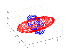
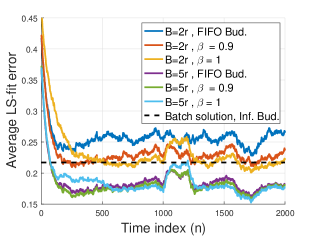
Refer to caption
Figure 4: Visualization of the nonlinear synthetic manifolds
Refer to caption
Figure 5: LS-fitting error of dynamic dataset versus time

Average mismatch of 𝐊^^𝐊\hat{{\bf K}} found from OK-FEB for various values of rank r𝑟r and choice of B=2r𝐵2𝑟B=2r is plotted in Fig. 6, and is compared with KPCA as well as state-of-the-art variations of the Nystrom approximation, namely Improved Nystrom [54], SS-Nystrom [48], and MEKA [44]. Considering the dynamic nature of the data, the mismatch is evaluated over a moving window of length Nwind=100subscript𝑁𝑤𝑖𝑛𝑑100N_{wind}=100, and averaged over all such windows. As the plot suggests, OK-FEB outperforms competing alternatives and better suites datasets with dynamic subspaces.
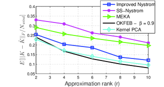
Refer to caption
Figure 6: Average kernel mismatch of dynamic data

VII-C Real-data on physical activity tracking

In this subsection, we test performance of OK-FEB on the physical activity monitoring dataset PAMAP2 [36]. The dataset contains N=129,200𝑁129200N=129,200 measurements from 3 Colibri wireless inertial measurement units (MU) worn by 9 subjects during different physical activities, such as walking and cycling. The MUs are placed on the dominant arm, chest, and dominant ankle of the subjects, each recording 13 quantities including acceleration and gyroscope data with sampling frequency 100Hz. We discarded all measurement vectors with missing entries, idle state measurements, and first and last 1,00010001,000 measurements of each activity, as they correspond to transient states. The tests are performed on data corresponding to subject number 1, and can be similarly repeated for other subjects as well.

The data is fed to OK-FEB with (r,B)=(10,15)𝑟𝐵1015(r,B)=(10,15), and step size set to μt=1/𝐪t2subscript𝜇𝑡1subscriptnormsubscript𝐪𝑡2\mu_{t}=1/\|{\bf q}_{t}\|_{2}. LS error given by the nonlinear feature extraction (averaged over a window of length 200 for improved visualization) is plotted in Fig. 7 across time. Every activity is also coded to a number in (0,1]01(0,1], and plotted in the same figure versus time to highlight the activity changes over time. As the figure illustrates, different activities correspond to different manifolds, each of which can be approximated with a certain accuracy via dynamic subspace learning and feature extraction. Introducing the forgetting factor β<1𝛽1\beta<1 enhances the learning capability. Table I reports the average LS-error and its variance for different activities using various budget maintenance strategies, with β=1,0.9𝛽10.9\beta=1,0.9, and the FIFO strategy.

Refer to caption
Figure 7: LS-fitting error of the PAMAP2 dataset versus time
TABLE I: Mean and variance of LS-fitting error of the extracted features with (r,B)=(10,15)𝑟𝐵1015(r,B)=(10,15) for different activities using different budget maintenance strategies
Code Activity β=1𝛽1\beta=1 β=0.9𝛽0.9\beta=0.9 FIFO Bud.
0.3 Walking 0.0990.0990.099 0.0740.0740.074 0.0740.0740.074
±0.016plus-or-minus0.016\pm 0.016 ±0.012plus-or-minus0.012\pm 0.012 ±0.012plus-or-minus0.012\pm 0.012
0.4 Running 0.2270.2270.227 0.1870.1870.187 0.1870.1870.187
±0.025plus-or-minus0.025\pm 0.025 ±0.022plus-or-minus0.022\pm 0.022 ±0.022plus-or-minus0.022\pm 0.022
0.5 Cycling 0.0580.0580.058 0.0280.0280.028 0.0280.0280.028
±0.027plus-or-minus0.027\pm 0.027 ±0.012plus-or-minus0.012\pm 0.012 ±0.12plus-or-minus0.12\pm 0.12
0.6 Nordic 0.1300.1300.130 0.1030.1030.103 0.1030.1030.103
Walking ±0.020plus-or-minus0.020\pm 0.020 ±0.016plus-or-minus0.016\pm 0.016 ±0.016plus-or-minus0.016\pm 0.016
0.7 Ascending 0.0790.0790.079 0.0630.0630.063 0.0630.0630.063
Stairs ±0.022plus-or-minus0.022\pm 0.022 ±0.018plus-or-minus0.018\pm 0.018 ±0.018plus-or-minus0.018\pm 0.018
0.8 Descending 0.0940.0940.094 0.0660.0660.066 0.0650.0650.065
Stairs ±0.021plus-or-minus0.021\pm 0.021 ±0.016plus-or-minus0.016\pm 0.016 ±0.016plus-or-minus0.016\pm 0.016
0.9 Vacuum 0.0450.0450.045 0.0290.0290.029 0.0290.0290.029
cleaning ±0.013plus-or-minus0.013\pm 0.013 ±0.008plus-or-minus0.008\pm 0.008 ±0.008plus-or-minus0.008\pm 0.008
1.0 Rope 0.2720.2720.272 0.2380.2380.238 0.2380.2380.238
jumping ±0.063plus-or-minus0.063\pm 0.063 ±0.057plus-or-minus0.057\pm 0.057 ±0.057plus-or-minus0.057\pm 0.057

Similar to Fig. 6, Fig. 8 depicts the average mismatch of kernel matrix approximation of OK-FEB with B=1.5r𝐵1.5𝑟B=1.5r for the PAMAP2 dataset. Comparison with the competing Nystrom variations in [54] and [44] clearly demonstrates the advantage of OK-FEB with forgetting factor β=0.9𝛽0.9\beta=0.9. Due to the large number of data vectors, KPCA and SS-Nystrom could not be implemented.
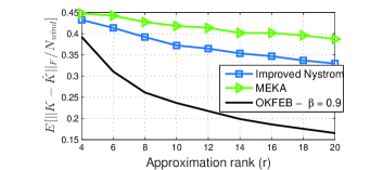
Refer to caption
Figure 8: Average kernel mismatch of PAMAP2 dataset

VII-D Online regression and classification

In this subsection, the generalization capability of the online linear classification and regression modules based on the features 𝐙𝐙{\bf Z} returned by OK-FEB is tested. We compare the performance of linear regression and classification as well as competing online kernel-based learners including (unbudgeted) Perceptron [15], (unbudgeted) Norma [21], (unbudgeted) online gradient descent (OGD) [41], (unbudgeted) online dictionary learning (ODL), and budgeted online gradient descent (BOGD) [49], Forgetron [10], Projectron [32], and budgeted passive-aggressive algorithm (BPA) [51] with our novel OK-FEB, where the acquired features 𝐳nsubscript𝐳𝑛{\bf z}_{n} are fed to online linear Pegasus[41] and regularized-LMS solvers for the classification and regression tasks, respectively. The size and specifications of the dataset used are listed in Table II, and are accessible from the LIBSVM website222http://www.csie.ntu.edu.tw/~cjlin/libsvmtools/ or the UCI machine learning repository 333http://www.ics.uci.edu/~mlearn/. The parameter values used per dataset are reported in Table II. In particular, tuning of the Frobenious norm regularization and kernel bandwidth parameters are done via cross validation over a discretized grid. Regarding the budget, to ensure stability of the algorithm it suffices that we set B>r𝐵𝑟B>r, while it has been observed that setting B𝐵B very high yields only marginal improvement in terms of accuracy. Finally, for the selection of r𝑟r, we test an increasing sequence of values starting from r=2𝑟2r=2 and gradually increasing until the improvement in terms of fitting error becomes negligible. The aforementioned process is typically used to determine the minimum required complexity of parametric models (e.g., order-adaptive least-squares [19]). The censoring threshold ϵitalic-ϵ\epsilon is set using a moving-average of LS-error values for the past 100100100 data vectors.

TABLE II: Specifications of datasets.
dataset D𝐷D N𝑁N r𝑟r B𝐵B γ𝛾\gamma C𝐶C
Adult 123 32K 505050 1.2r1.2𝑟1.2r 202020 101010
CADATA 8 20.6K 555 1,5r15𝑟1,5r 7×1077superscript1077\times 10^{7} 0.010.010.01
Slice 384 53.5K 101010 1.2r1.2𝑟1.2r 505050 0.010.010.01
Year 90 463.7K 101010 1.2r1.2𝑟1.2r 5×1075superscript1075\times 10^{7} 0.010.010.01

Classification and regression accuracy as well as run time are plotted versus iteration index. Perceptron, Norma, ODL, and OGD are unbudgeted algorithms, and their SV sets (dictionary atoms in ODL) grow as iteration index increases in Fig. 9. Although the accuracy of these algorithms can serve as a benchmark, their run time grows the fastest. Thus, for the “Year” dataset (Nmuch-greater-than𝑁absentN\gg), the mentioned algorithms are run only over 10%percent1010\% of the data vectors. As these tests demonstrate, among the budgeted algorithms, OK-FEB reliably approximates the kernel function through the extracted features, thus offering more accurate classification and regression performance when compared to existing alternatives.
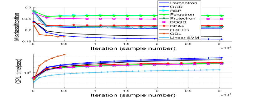
Refer to caption

(a)

Refer to caption

(b)

Refer to caption

(c)

Refer to caption

(d)

Figure 9: Online classification tests on (a) Adult, and regression tests on (b) CADATA, (c) Slice, and (d) Year datasets.

VIII Concluding Remarks

Low-complexity feature extraction algorithms were introduced in this paper to markedly improve performance of kernel-based learning methods applied to large-scale datasets. The novel approach begins with a generative model having data mapped to a high-(possibly infinite-) dimensional space, where they lie close to a linear low-rank subspace, the tracking of which enables effective feature extraction on a budget. The extracted features can be used by fast linear classifiers or regression predictors at scale.

Offline and online solvers of the subspace learning task were developed, and their convergence was studied analytically. To keep the complexity and memory requirements within affordable levels, budgeted algorithms were devised, in which the number of stored data vectors is restricted to a prescribed budget. Further analysis provided performance bounds on the quality of the resultant kernel matrix approximation, as well as the precision with which kernel-based classification and regression tasks can be approximated by leveraging budgeted online subspace-learning and feature-extraction tasks.

Finally, online subspace tracking and nonlinear feature extraction for dynamic datasets as well as classification and regression tests on synthetic and real datasets demonstrated the efficiency of OK-FEB with respect to competing alternatives, in terms of both accuracy and run time.

IX Appendix

Proof of Proposition 2: The proof of the proposition is inspired by [28] and [27], and is sketched along the following steps.

Step 1. First, we judiciously introduce a surrogate for Fn(𝐋¯)subscript𝐹𝑛¯𝐋F_{n}(\bar{\bf L}) whose minimizer coincides with the SGD updates in (13).

To this end, we have that min𝐪fν(𝐱ν;𝐋¯,𝐪)fν(𝐱ν;𝐋¯,𝐪[ν])subscript𝐪subscript𝑓𝜈subscript𝐱𝜈¯𝐋𝐪subscript𝑓𝜈subscript𝐱𝜈¯𝐋𝐪delimited-[]𝜈\min_{{\bf q}}{f_{\nu}}({\bf x}_{\nu};\bar{\bf L},{\bf q})\leq{f_{\nu}}({\bf x}_{\nu};\bar{\bf L},{\bf q}[\nu]); hence, F^n(𝐋¯):=(1/n)ν=1nfν(𝐱ν;𝐋¯,𝐪[ν])assignsubscript^𝐹𝑛¯𝐋1𝑛superscriptsubscript𝜈1𝑛subscript𝑓𝜈subscript𝐱𝜈¯𝐋𝐪delimited-[]𝜈\hat{F}_{n}(\bar{\bf L}):=(1/n)\sum_{\nu=1}^{n}f_{\nu}({\bf x}_{\nu};\bar{\bf L},{\bf q}[\nu]) upper bounds the cost function, namely Fn(𝐋¯)F^n(𝐋¯),𝐋¯subscript𝐹𝑛¯𝐋subscript^𝐹𝑛¯𝐋for-all¯𝐋F_{n}(\bar{\bf L})\leq\hat{F}_{n}(\bar{\bf L}),\;\forall\bar{{\bf L}}. Further approximating fnsubscript𝑓𝑛f_{n} through a second-order Taylor’s expansion at the previous subspace update 𝐋¯[n1]¯𝐋delimited-[]𝑛1\bar{\bf L}[n-1], we arrive at

f~n(𝐱n;𝐋¯,𝐪[n])subscript~𝑓𝑛subscript𝐱𝑛¯𝐋𝐪delimited-[]𝑛\displaystyle\tilde{f}_{n}({\bf x}_{n};\bar{\bf L},{\bf q}[n]) =fn(𝐱n;𝐋¯[n1],𝐪[n])absentsubscript𝑓𝑛subscript𝐱𝑛¯𝐋delimited-[]𝑛1𝐪delimited-[]𝑛\displaystyle=f_{n}({\bf x}_{n};\bar{\bf L}[n-1],{\bf q}[n]) (42)
+tr{𝐋¯fn(𝐱n;𝐋¯[n1],𝐪[n])(𝐋¯𝐋¯[n1])}trsubscript¯𝐋subscript𝑓𝑛subscript𝐱𝑛¯𝐋delimited-[]𝑛1𝐪delimited-[]𝑛superscript¯𝐋¯𝐋delimited-[]𝑛1top\displaystyle+\text{tr}\{\nabla_{\bar{\bf L}}f_{n}({\bf x}_{n};\bar{\bf L}[n-1],{\bf q}[n])(\bar{\bf L}-\bar{\bf L}[n-1])^{\top}\}
+γn2𝐋¯𝐋¯[n1]HS2.subscript𝛾𝑛2superscriptsubscriptnorm¯𝐋¯𝐋delimited-[]𝑛1𝐻𝑆2\displaystyle+\dfrac{\gamma_{n}}{2}\|\bar{\bf L}-\bar{\bf L}[n-1]\|_{HS}^{2}\;.

By choosing γn𝐋¯2fn(𝐱n;𝐋¯[n1],𝐪n)=(𝐪[n]𝐪[n])𝐈D¯+(λ/n)𝐈rD¯subscript𝛾𝑛subscriptnormsubscriptsuperscript2¯𝐋subscript𝑓𝑛subscript𝐱𝑛¯𝐋delimited-[]𝑛1subscript𝐪𝑛subscriptnormtensor-product𝐪delimited-[]𝑛superscript𝐪topdelimited-[]𝑛subscript𝐈¯𝐷𝜆𝑛subscript𝐈𝑟¯𝐷\gamma_{n}\geq\|\nabla^{2}_{\bar{\bf L}}f_{n}({\bf x}_{n};\bar{\bf L}[n-1],{\bf q}_{n})\|_{\mathcal{H}}=\|({\bf q}[n]{\bf q}^{\top}[n])\otimes\mathbf{I}_{\bar{D}}+(\lambda/n)\mathbf{I}_{r\bar{D}}\|_{\mathcal{H}} and using the norm properties in the Hilbert space, the following can be verified:

(i) f~nsubscript~𝑓𝑛\tilde{f}_{n} is locally tight; i.e., f~n(𝐱n;𝐋¯[n1],𝐪[n])=fn(𝐱n;𝐋¯[n1],𝐪[n])subscript~𝑓𝑛subscript𝐱𝑛¯𝐋delimited-[]𝑛1𝐪delimited-[]𝑛subscript𝑓𝑛subscript𝐱𝑛¯𝐋delimited-[]𝑛1𝐪delimited-[]𝑛\tilde{f}_{n}({\bf x}_{n};\bar{\bf L}[n-1],{\bf q}[n])={f}_{n}({\bf x}_{n};\bar{\bf L}[n-1],{\bf q}[n]);

(ii) gradient of f~nsubscript~𝑓𝑛\tilde{f}_{n} is locally tight; i.e., 𝐋¯f~n(𝐱n;𝐋¯[n1],𝐪[n])=𝐋¯fn(𝐱n;𝐋¯[n1],𝐪[n])subscript¯𝐋subscript~𝑓𝑛subscript𝐱𝑛¯𝐋delimited-[]𝑛1𝐪delimited-[]𝑛subscript¯𝐋subscript𝑓𝑛subscript𝐱𝑛¯𝐋delimited-[]𝑛1𝐪delimited-[]𝑛\nabla_{\bar{\bf L}}\tilde{f}_{n}({\bf x}_{n};\bar{\bf L}[n-1],{\bf q}[n])=\nabla_{\bar{\bf L}}{f}_{n}({\bf x}_{n};\bar{\bf L}[n-1],{\bf q}[n]); and

(iii) f~nsubscript~𝑓𝑛\tilde{f}_{n} globally majorizes the original instantaneous cost fnsubscript𝑓𝑛f_{n}; that is, fn(𝐱n;𝐋¯,𝐪[n])f~n(𝐱n;𝐋¯,𝐪[n])subscript𝑓𝑛subscript𝐱𝑛¯𝐋𝐪delimited-[]𝑛subscript~𝑓𝑛subscript𝐱𝑛¯𝐋𝐪delimited-[]𝑛f_{n}({\bf x}_{n};\bar{\bf L},{\bf q}[n])\leq\tilde{f}_{n}({\bf x}_{n};\bar{\bf L},{\bf q}[n]), 𝐋¯for-all¯𝐋\forall\,\bar{\bf L}.

Selecting now the target surrogate cost as F~n(𝐋¯)=1nν=1nf~ν(𝐱ν;𝐋¯,𝐪[ν])subscript~𝐹𝑛¯𝐋1𝑛superscriptsubscript𝜈1𝑛subscript~𝑓𝜈subscript𝐱𝜈¯𝐋𝐪delimited-[]𝜈\tilde{F}_{n}(\bar{\bf L})=\dfrac{1}{n}\sum_{\nu=1}^{n}\tilde{f}_{\nu}({\bf x}_{\nu};\bar{\bf L},{\bf q}[\nu]) we have Fn(𝐋¯)F^n(𝐋¯)F~n(𝐋¯),𝐋¯formulae-sequencesubscript𝐹𝑛¯𝐋subscript^𝐹𝑛¯𝐋subscript~𝐹𝑛¯𝐋for-all¯𝐋F_{n}(\bar{\bf L})\leq\hat{F}_{n}(\bar{\bf L})\leq\tilde{F}_{n}(\bar{\bf L}),\forall\,\bar{\bf L}. Minimizing the cost F~n(𝐋¯)subscript~𝐹𝑛¯𝐋\tilde{F}_{n}(\bar{\bf L}) amounts to nullifying the gradient, i.e., 𝐋¯F~n(𝐋¯[n])=𝟎subscript¯𝐋subscript~𝐹𝑛¯𝐋delimited-[]𝑛0\nabla_{\bar{{\bf L}}}\tilde{F}_{n}(\bar{{\bf L}}[n])=\mathbf{0}, which yields [28] 𝐋¯[n]=𝐋¯[n1]γ¯n1𝐆¯n¯𝐋delimited-[]𝑛¯𝐋delimited-[]𝑛1superscriptsubscript¯𝛾𝑛1subscript¯𝐆𝑛\bar{\bf L}[n]=\bar{\bf L}[n-1]-{\bar{\gamma}_{n}}^{-1}\bar{\bf G}_{n}, with γ¯n:=ν=1nγνassignsubscript¯𝛾𝑛superscriptsubscript𝜈1𝑛subscript𝛾𝜈\bar{\gamma}_{n}:=\sum_{\nu=1}^{n}\gamma_{\nu}. By setting μn=1/γ¯nsubscript𝜇𝑛1subscript¯𝛾𝑛\mu_{n}=1/\bar{\gamma}_{n}, the SGD-based update of 𝐋¯[n]¯𝐋delimited-[]𝑛\bar{\bf L}[n] now coincides with the minimizer of F~n(𝐋¯)subscript~𝐹𝑛¯𝐋\tilde{F}_{n}(\bar{\bf L}); that is, 𝐋¯[n]=argmin𝐋¯F~n(𝐋¯)¯𝐋delimited-[]𝑛subscript¯𝐋subscript~𝐹𝑛¯𝐋\bar{\bf L}[n]=\arg\min_{\bar{\bf L}}\tilde{F}_{n}(\bar{\bf L}).

Step 2. The second step establishes that the surrogate costs {F~n(𝐋¯)}subscript~𝐹𝑛¯𝐋\{\tilde{F}_{n}(\bar{\bf L})\} form a quasi-martingale sequence [24], and using tightness of the surrogate cost we deduce that limn(Fn(𝐋¯[n])F~n(𝐋¯[n]))=0subscript𝑛subscript𝐹𝑛¯𝐋delimited-[]𝑛subscript~𝐹𝑛¯𝐋delimited-[]𝑛0\lim_{n\rightarrow\infty}(F_{n}(\bar{\bf L}[n])-\tilde{F}_{n}(\bar{\bf L}[n]))=0. Thus, the surrogate cost asymptotically converges to the original cost Fn(𝐋¯)subscript𝐹𝑛¯𝐋F_{n}(\bar{\bf L}).

Step 3. Leveraging the regularity of ¯(𝐱ν;𝐋¯,𝐪ν)¯subscript𝐱𝜈¯𝐋subscript𝐪𝜈\bar{\cal L}({\bf x}_{\nu};\bar{\bf L},{\bf q}_{\nu}), convergence of the cost sequence implies convergence of {𝐋¯Fn(𝐋¯[n])𝐋¯F~n(𝐋¯[n])𝒮}subscriptnormsubscript¯𝐋subscript𝐹𝑛¯𝐋delimited-[]𝑛subscript¯𝐋subscript~𝐹𝑛¯𝐋delimited-[]𝑛𝒮\{\|\nabla_{\bar{\bf L}}F_{n}(\bar{\bf L}[n])-\nabla_{\bar{\bf L}}\tilde{F}_{n}(\bar{\bf L}[n])\|_{\cal{HS}}\} to zero, which along with 𝐋¯F~n(𝐋¯[n])=𝟎subscript¯𝐋subscript~𝐹𝑛¯𝐋delimited-[]𝑛0\nabla_{\bar{{\bf L}}}\tilde{F}_{n}(\bar{{\bf L}}[n])=\mathbf{0}, yields {𝐋¯Fn(𝐋¯[n])𝒮}𝟎subscriptnormsubscript¯𝐋subscript𝐹𝑛¯𝐋delimited-[]𝑛𝒮0\{\|\nabla_{\bar{\bf L}}F_{n}(\bar{\bf L}[n])\|_{\cal{HS}}\}\rightarrow\mathbf{0}. \hfill\blacksquare

References

  • [1] F. Bach, “Sharp analysis of low-rank kernel matrix approximations,” Conference on Learning Theory, pp. 185-209, Princeton, NJ, June 2013.
  • [2] F. Bach, G. Lanckriet, and M. Jordan, “Multiple kernel learning, conic duality, and the SMO algorithm,” Proc. of Intl. Conf. on Mach. Learn., Alberta, Canada, June 2004.
  • [3] D. P. Bertsekas, Nonlinear Programming, Athena Scientific, 1999.
  • [4] D. Berberidis, V. Kekatos, and G.B. Giannakis, “Online Censoring for Large-Scale Regressions with Application to Streaming Big Data,” IEEE Trans. on Signal Proc., vol. 64, pp. 3854-3867, Aug. 2016.
  • [5] A. Bordes, S. Ertekin, J. Weston, and L. Bottou, “Fast kernel classifiers with online and active learning,” J. of Mach. Learn. Res., vol. 6, pp. 1579-1619, Sept. 2005.
  • [6] G. Cavallanti, N. Cesa-Bianchi, and C. Gentile, “Tracking the best hyperplane with a simple budget perceptron,” Machine Learning, vol. 69, pp. 143-167, Dec. 2007.
  • [7] C. C. Chang and C. J. Lin, “LIBSVM: A library for support vector machines,” ACM Trans. Intelligent Systems and Technology, vol. 2, no. 3, pp. 27:1-27:27, Apr. 2011.
  • [8] C. Cortes, M. Mohri, and A. Talwalkar, “On the impact of kernel approximation on learning accuracy,” Proc. of Intl. Conf. on Artif. Intel. and Stat., pp. 113-120, Sardinia, Italy, May 2010.
  • [9] B. Dai, B. Xie, N. He, Y. Liang, A. Raj, M. F. Balcan, and L. Song, “Scalable kernel methods via doubly stochastic gradients,” Proc. of NIPS, pp. 3041-3049, Montreal, Canada, Dec. 2014.
  • [10] O. Dekel, S. Shalev-Shwartz, and Y. Singer, “The forgetron: A kernel-based perceptron on a budget,” SIAM J. on Computing, vol. 37, no. 5, pp. 1342-1372, Dec. 2008.
  • [11] O. Dekel, and Y. Singer, “Support vector machines on a budget,” Proc. of NIPS, pp. 345-352, Vancouver, Canada, Dec. 2007.
  • [12] P. Drineas, M. W. Mahoney, “On the Nystrom method for approximating a Gram matrix for improved kernel-based learning,” J. of Mach. Learn. Res., vol. 6, pp. 2153-2175, Dec. 2005.
  • [13] R. E. Fan, K. W. Chang, C. J. Hsieh, X. R. Wang, and C. J. Lin, “LIBLINEAR: A Library for Large Linear Classification,” J. of Mach. Learn. Res., vol. 9, pp. 1871-1874, Apr. 2008.
  • [14] S. Fine, and K. Scheinberg, “Efficient SVM training using low-rank kernel representations,” J. of Mach. Learn. Res., vol. 2, pp. 243-264, Dec. 2002.
  • [15] Y. Freund, R. E. Schapire, “Large margin classification using the perceptron algorithm,” Machine Learning, vol. 37, pp. 277-296, Dec. 1999.
  • [16] R. Gribonval, R. Jenatton, F. Bach, M. Kleinsteuber, M. Seibert, “Sample complexity of dictionary learning and other matrix factorizations,” IEEE Trans. on Info. Theory , vol. 61, pp. 3469-3486, June 2015.
  • [17] Y. Hastie, R. Tibshirani, and J. Friedman, The Elements of Statistical Learning, Springer, 2008.
  • [18] P. Honeine, “Online kernel principal component analysis: A reduced-order model,” IEEE Trans. on Patt. Anal. and Mach. Intel., vol. 34, pp. 1814-1826, Sept. 2012.
  • [19] S. Kay, Fundamentals of statistical signal processing, Prentice Hall PTR, 1993.
  • [20] K. Kim, M. Franz, and B. Scholkopf, “Iterative principal component analysis for image modeling,” IEEE Trans. on Patt. Anal. and Mach. Intl., vol. 27, pp. 1351-1366, Sept. 2005.
  • [21] J. Kivinen, A. Smola, and R. Williamson, “Online learning with kernels,” IEEE Trans. on Sign. Proc., vol. 52, pp. 2165-2176, Aug. 2004.
  • [22] S. Kumar, M. Mohri, and A. Talwalkar, “Ensemble Nystrom method,” Proc. of NIPS, pp. 1060-1068, Vancouver, Canada, Dec. 2009.
  • [23] Y. J. Lee, and O.L. Mangasarian, “RSVM: Reduced Support Vector Machines,” Proc. of SIAM Intl. Conf. on Data Mining, vol. 1, pp. 325-361, Chicago, April 2001.
  • [24] L. Ljung and T. Soderstrom Theory and Practice of Recursive Identification, 2nd ed. MIT Press, 1983.
  • [25] D. Lopez-Paz, S. Sra, A. Smola, Z. Ghahramani, and B. Scholkopf, “Randomized nonlinear component analysis,” Proc. of Intl. Conf. on Mach. Learn., pp. 1359-1367, Beijing, China, June 2014.
  • [26] J. Lu, S. C. H. Hoi, J. Wang, P. Zhao, Z. Liu, “Large scale online kernel learning,” J. of Mach. Learn. Res., vol. 17, pp. 1−-43, Jan. 2016.
  • [27] J. Mairal, F. Bach, J. Ponce, and G. Sapiro, “Online learning for matrix factorization and sparse coding,” J. of Mach. Learn. Res., vol. 11, pp. 19-60, March 2011.
  • [28] M. Mardani, G. Mateos, and G. B. Giannakis, “Dynamic anomalography: Tracking network anomalies via sparsity and low-rank,” IEEE J. Sel. Topics in Sig. Proc., vol. 7, no. 1, pp. 50-66, Feb. 2013.
  • [29] M. Mardani, G. Mateos, and G. B. Giannakis, “Decentralized sparsity-regularized rank minimization: Algorithms and applications,” IEEE Tran. on Sig. Proc., vol. 61, no. 21, pp. 5374–5388, Nov. 2013.
  • [30] A. Maurer, M. Pontil, “K-Dimensional Coding Schemes in Hilbert Spaces,” IEEE Trans. on Info. Theory, vol. 56, pp. 5839-5846, Nov. 2010.
  • [31] A. Nemirovski, J. Anatoli, L. G. Lan, and A. Shapiro, “Robust stochastic approximation approach to stochastic programming,” SIAM J. on Optim., vol. 19, pp. 1574-1609, Jan. 2009.
  • [32] F. Orabona, J. Keshet, B. Caputo, “The projectron: A bounded kernel-based perceptron,” Proc. of Intl. Conf. on Mach. Learn., pp. 720-727, Chicago, July 2011.
  • [33] A. Rahimi and B. Recht, “Random features for large-scale kernel machines,” Proc. of Advances in Neural Inf. Proc. Systems, pp. 1177-1184, Lake Tahoe, Dec. 2013.
  • [34] A. Rakotomamonjy, F. Bach, S. Canu, and Y. Grandvalet, “More efficiency in multiple kernel learning,” Proc. of Intl. Conf. Mach. Learn., pp. 775–782, Corvallis, USA, June 2007.
  • [35] B. Recht, M. Fazel, and P. A. Parrilo, “Guaranteed minimum-rank solutions of linear matrix equations via nuclear norm minimization,” SIAM Rev., vol. 52, pp. 471-501, Aug. 2010.
  • [36] A. Reiss, and D. Stricker, “Introducing a new Benchmarked dataset for activity monitoring,” IEEE Intl. Symp. on Wearable Computers, Newcastle, United Kingdom, June 2012.
  • [37] R. Rubinstein, M. Zibulevsky, M. Elad, “Double sparsity: Learning sparse dictionaries for sparse signal approximation,” IEEE Trans. on Sig.nal Proc., vol. 58, pp. 1553-1564, March 2010.
  • [38] B. Scholkopf, and A. J. Smola, Learning with Kernels: Support Vector Machines, Regularization, Optimization, and beyond, MIT Press, 2001.
  • [39] B. Scholkopf, A. Smola, and K. R. Muller, “Nonlinear component analysis as a kernel eigenvalue problem,” Neural Computation, vol. 10.5, pp. 1299-1319, July 1998.
  • [40] N. Schraudolph, S. Gunter, and S. V. N. Vishwanathan, “Fast iterative kernel principal component analysis,” J. of Mach. Learn. Res., vol. 8, pp. 1893-1918, Aug. 2008.
  • [41] S. Shalev-Shwartz, Y. Singer, N. Srebro, and A. Cotter, “Pegasos: Primal estimated sub-gradient solver for SVM,” Mathematical Programming, Springer, vol. 127, no. 1, pp. 3-30, March 2011.
  • [42] F. Sheikholeslami, and G. B. Giannalis, “Scalable kernel-based learning via low-rank approximation of lifted data,” Proc. of Allerton Conf. on Comm., Control, and Computing, Urbana, IL, Oct. 2017.
  • [43] F. Sheikholeslami, D. Berberidis, and G. B. Giannakis, “Memory efficient low-rank nonlinear subspace tracking,” Proc. of CAMSAP, Curacao, Dutch Antilles, Dec. 2017.
  • [44] S. Si, C. J. Hsieh, and I. S. Dhillon “Memory efficient kernel approximation,” Proc. of Intl. Conf. on Mach. Learn., pp. 701-709, Beijing, China, June 2014.
  • [45] I. W. Tsang, J. T. Kwok, and P. M. Cheung. “Core vector machines: Fast SVM training on very large data sets,” J. of Mach. Learn. Res., pp. 363-392, Apr. 2005.
  • [46] D. Vainsencher, S. Mannor, A. M. Bruckstein, “The sample complexity of dictionary learning,” J. of Mach. Learn. Res., vol. 12, pp. 3259-3281, Nov. 2011.
  • [47] S. Van Vaerenbergh, I. Santamaria, W. Liu, and J. C. Principe, “Fixed-budget kernel recursive least-squares,” Proc of Intl. Conf. on Acoust., Speech and Sig. Proc., pp. 1882-1885, Dallas, TX, Mar. 2010.
  • [48] S. Wang, C. Zhang, H. Qian, Z. Zhang, “Improving the modified nyström method using spectral shifting,” Proc. of KDD, pp. 611-620, New York, Aug. 2014.
  • [49] Z. Wang, K. Crammer, and S. Vucetic, “Breaking the curse of kernelization: Budgeted stochastic gradient descent for large scale SVM training,” J. of Mach. Learn. Res., vol. 13, pp. 3103-3131, June 2012.
  • [50] Z. Wang, and S. Vucetic, “Online training on a budget of support vector machines using twin prototypes,” Statistical Analysis and Data Mining: The ASA Data Science Journal, vol. 3, pp. 149-169, June 2010.
  • [51] Z. Wang, and S. Vucetic, “Online passive-aggressive algorithms on a budget,” J. of Mach. Learn. Res., vol. 9, pp. 908-915, March 2010.
  • [52] C. Williams, and M. Seeger, “Using the Nystrom method to speed up kernel machines,” Proc. of Advances on NIPS, pp. 682-688, Vancouver, Canada, Dec. 2001.
  • [53] K. Zhang, L. Lan, Z. Wang, and F. Moerchen, “Scaling up kernel SVM on limited resources: A low-rank linearization approach,” Proc. of Intl. Conf. on Artif. Intel. and Stat., pp. 1425-1434, La Palma, Canary Islands, April 2012.
  • [54] K. Zhang, I. Tsang, and J. Kwok, “Improved Nystrom low-rank approximation and error analysis,” Proc. of Intl. Conf. on Mach. Learn., pp. 1232-1239, Helsinki, Finland, July 2008.
  • [55] T. Yang, Y. Li, M. Mahdavi, R. Jin, and Z. Zhou, “Nystrom method vs random Fourier features: A theoretical and empirical comparison,” Proc. of NIPS, pp. 476-484, Lake Tahoe, Dec. 2012.