Abstract

Many models and real complex systems possess critical thresholds at which the systems shift from one sate to another. The discovery of the early warnings of the systems in the vicinity of critical point are of great importance to estimate how far a system is from a critical threshold. Multifractal Detrended Fluctuation analysis (MF-DFA) and visibility graph method have been employed to investigate the fluctuation and geometrical structures of magnetization time series of two-dimensional Ising model around critical point. The Hurst exponent has been confirmed to be a good indicator of phase transition. Increase of the multifractality of the time series have been observed from generalized Hurst exponents and singularity spectrum. Both Long-term correlation and broad probability density function are identified to be the sources of multifractality of time series near critical regime. Heterogeneous nature of the networks constructed from magnetization time series have validated the fractal properties of magnetization time series from complex network perspective. Evolution of the topology quantities such as clustering coefficient, average degree, average shortest path length, density, assortativity and heterogeneity serve as early warnings of phase transition. Those methods and results can provide new insights about analysis of phase transition problems and can be used as early warnings for various complex systems.

Introduction

Complex systems are consisted with subunits that interact non-linearly with each other. Among so many general properties which describe the complex systems, the existence of critical threshold is apparently common to plenty of complex systems[44]. It is not possible to fully anticipate the behaviour of the system in terms of behaviours of its components. Thus characterizing the dynamical process of a complex system from time series is a fundamental problem of significant importance in many research fields[55, 27]. Here we focus on the very well known physical system, two-dimensional Ising model[18, 6]. It is a statistical physics model for ferromagnetic materials which goes through phase transition at non-zero temperature. The Ising model has been widely applied to different fields such as social systems[8] and financial systems[47]. We use the Metropolis algorithm[35]to simulate two-dimensional Ising system. The output of the simulation are time series of average magnetization of the system at different temperature. Time evolution of average magnetization can be used to reveal the dynamical properties of the system.

Fractals and mutifractals are ubiquitous in physics and social systems[33]. Time series are the most common fractal objects in most of the scientific research fields. Lots of techniques have been proposed to analyze the fractal and multifractal properties of time series[41, 23, 24, 57, 42, 15, 21]. Multifractal detrended fluctuation analysis(MF-DFA)[24] we adopted here has shown to be a quite effective tool to investigate the multifractal properties of non-stationary time series. Also the complex network[1] is one of the generic ways to describe complex systems. Transformations from time series to networks have attracted substantial considerations recently[51, 55, 29, 56]. It has been shown that the visibility graph method[29] is suitable for characterizing the correlation and geometrical structure of time series[28].

Recently there has been an substantial interest in understanding how those complex systems behave near the critical point. Lots of early warnings have been discovered to serve as a signals of the coming of the tipping points[44]. In this paper, we use the MF-DFA and the visibility graph method to analyze the behaviour of the Ising system near critical temperature. The level of the mutifractality of the time series and topological quantities of the complex networks converted from time series can bee seen as some new early warnings. Hurst exponents increase dramatically around critical point which means the time series change from a weak correlated to long term correlated ones. Generalized Hurst exponents have shown the transformation of fractal structures of the time series from weak multifractal (or monofractal) to multifractal while the system approaches to critical regime. These indicate huge differences between the dynamical behaviours of Ising system at different temperatures. Evolution of the singularity spectrum has depicted the extreme strong multifractality around critical point. Structure parameters of the singularity spectrum suggest that the time series become much more complex around critical point. The shuffling procedure reveals that both broad probability density function and long term correlations are the sources of multifractality of the magnetization time series around critical point. Visibility graphs converted from the time series at different temperature share the heterogeneous property which is consist with the previous results: fractal time series can be converted to scale-free networks[29]. We also find that the increase and decrease of the topological quantities can be used to identify the coming of phase transition. The evolution behaviours of topological structures of the visibility graphs have manifested the differences among geometrical structures of magnetization time series at different temperature regimes from network perspective.

Methods

Simulation of Ising model

The two-dimensional Ising model is a paradigm of physical phase transition. Suppose we have a square lattice of $N$ sites with periodic boundary conditions. A spin state $\sigma$ is defined on each site with one of two possible orientation values which denoted by $\sigma=\pm 1$. So the number of all possible configurations of the system is $2^{N}$. The Hamiltonian is

$$H(\sigma)=-\sum\limits_{<i,j>}J_{ij}\sigma_{i}\sigma_{j}-\mu\sum\limits_{i=1}^{N}h_{i}\sigma_{i}\qquad.$$ (1)

Any two adjacent sites $i,j\in N$ have an interaction strength $J_{ij}$. A site $i\in N$ has an external magnetic field $h_{i}$ acting on it and $\mu$ is the magnetic moment. Here we concern about the case while $J_{ij}=1$ and $h_{i}=0$. The order of the system can be measured through the magnetization per spin which defined as

$$M=\frac{1}{N}\sum\limits_{i=1}^{N}\sigma_{i}\qquad.$$ (2)

It is well known that for two-dimensional Ising model the system goes through a phase transition when temperature $T$ is equal to critical temperature $T_{c}$. There exists spontaneous magnetization as all the spins tend to equal towards either +1 state or -1 state at a non-zero critical temperature $T_{c}$.

Here in this paper we focus on the dynamics of the Ising model. Monte Carlo simulation by using Metropolis algorithm[35] is employed to capture the evolution of the system. Thus the time series of magnetization $M$ can be obtained from simulation procedure.

In the Metropolis algorithm, new configurations are generated from the previous state using a transition probability. The probability of the system being in a state $n$ follows the Boltzmann distribution:

$$P_{n}=\frac{e^{-E_{n}/kT}}{Z}$$ (3)

,where $E_{n}$ is the free energy of the state, $k$ is the Boltzmann constant, $T$ is temperature and $Z$ is the partition function. Thus the transition probability from state $n$ to $m$ is given by

$$P_{n\rightarrow m}=\mathrm{exp}[-\Delta E/kT]$$ (4)

,here $\Delta E=E_{m}-E_{n}$.

According to previous description, given an initial state of the system, the algorithm proceeds as follows:
1. Choose a site $i$ randomly;
2. Calculate the energy change $\Delta E$ if spin site $i$ were to be flipped;
3. If $\Delta E$ is negative, flip of the spin of site $i$ is accepted. If $\Delta E$ is positive, a random number is drawn between 0 and 1 uniformly and the flip is accepted only if the random number is smaller than $\mathrm{exp}[-\Delta E/kT]$;
4. Choose another site and repeat the previous steps.

A Monte Carlo step is completed when every spin of the system has had a chance to flip. In the ordinary simulation schematic, due to the phenomena of critical slowing down, when the system is around critical temperature $T_{c}$, one should skip several Monte Carlo steps in order to avoid correlations between successive configurations. This is important for evaluating the interested quantities accurately. On the contrary, here we keep all the time series of magnetization $M$ calculated from every simulation step. We are indeed very interested about the correlations and the properties caused by the critical slowing down phenomena.

We set $k=1$ and $J_{ij}=1$ which means the exact critical temperature $T_{c}\simeq 2.27$. We have simulated the system from $T=1.17$ to $T=3.62$ with $\Delta T=0.05$. For every discrete temperature we run an ensemble of 100 simulations of 100000 Monte Carlo steps(the first 10000 steps have been discarded to overcome the influence of the initial configuration). In order to investigate the finite size effect, we have simulated different lattice sizes for $N=100\times 100,150\times 150,200\times 200,300\times 300$.

By using the Metropolis algorithm, we have obtained a time series ensemble at different temperature. Then in the following section we will introduce two methods which used to analyze the properties of those time series from two different aspects: multifractal and complex network.

Mutifractal Detrended Fluctuation Analysis

We adopt multifractal detrended fluctuation analysis (MF-DFA) to analyze the hierarchy of scaling exponents of the magnetization time series corresponding to different scaling behaviour[24]. It is the generalization of detrended fluctuation analysis (DFA)[41]. The MF-DFA method have been widely applied to characterize the properties of various non-stationary time series from different fields such as financial market [20, 43, 26, 38, 40, 46, 37, 17, 48, 49], physiological[11], biology[10],traffic jamming[2], geophysics[50] and neuroscience[60].

The MF-DFA method is proceeded as follows: $(i)$ Suppose we have a time series $\{x(i)\},i=1,\ldots,l$. We first integrate the time series to get the profile $y(k)=\sum\limits_{i=1}^{k}[x(i)-\langle x\rangle],k=1,\ldots,l$, where $\langle x\rangle$ is the mean value of $\{x(i)\}$. $(ii)$ Divide the integrated series $y(k)$ into $l_{s}=int(l/s)$ non-overlapping segments of length $s$. Calculate the local trends for each of $l_{s}$ segments by a least-square fit and subtract it from $y(k)$ to detrend the integrated series. We get the detrended variance of each segment $v$

$$F^{2}(v,s)=\frac{1}{s}\sum\limits_{i=1}^{s}\{y(v-1+i)-\widetilde{y(v,i)}\}^{2}\qquad$$ (5)

,here $\widetilde{y(v,i)}$ is the fitting polynomial in segment $v=1,\ldots,l_{s}$. We use the three order polynomial fit here. $(iii)$ The step $(ii)$ has been proceed from both the beginning and the end of the time series which leads to $2l_{s}$ segments in total. Average over all segments to obtain the $q\mathrm{th}$ order fluctuation function

$$F_{q}(s)=\{\frac{1}{2l_{s}}\sum\limits_{v=1}^{2l_{s}}[F^{2}(v,s)]^{q/2}\}^{1/q}\qquad.$$ (6)

$(iv)$ Repeat this calculation to get the fluctuation function $F_{q}(s)$ for different box size $s$. If $F_{q}(s)$ increases by a power law $F_{q}(s)\sim s^{h(q)}$, the scaling exponents $h(q)$ (called generalized Hurst exponent) can estimated as the slope of the linear regression of $\mathrm{log}F_{q}(s)$ versus $\mathrm{log}s$. $h(q)$ is the fluctuation parameter and describe the correlation structures of the time series at different magnitude. The value of $h(0)$ can not be determined by using Eq(6) because of the diverging exponent. The logarithm averaging procedure should be used,

$$F_{0}(s)=\mathrm{exp}\{\frac{1}{4l_{s}}\sum\limits_{v=1}^{2l_{s}}\mathrm{ln}[F^{2}(v,s)]\}\sim s^{h(0)}\qquad.$$ (7)

Generalized Hurst exponents $h(q)$ as a function of the $q\mathrm{th}$ order can quantify the multifractality. If $h(q)$ are the same for all $q$, the time series is monofractal or the time series is mutifractal.

The classical multifractal scaling exponents[4]

$$\tau(q)=qh(q)-1$$ (8)

are directly related to the generalized Hurst exponents $h(q)$. Another way to characterize multifractal time series is by using the singularity spectrum $f(\alpha)$ which is related to $\tau(q)$ via the Legendre transform[24],

$$\alpha=\tau^{{}^{\prime}}(q),f(\alpha)=q\alpha-\tau(q)\qquad.$$ (9)

Using Eq(8), we have

$$\alpha=h(q)+qh^{{}^{\prime}}(q),f(\alpha)=q[\alpha-h(q)]+1\qquad.$$ (10)

Here $\alpha$ is the singularity strength. Geometrical shape of the singularity spectrum can illustrate the level of mutifractality from three parameters: position of the maximum $\alpha_{0}$ where $f(\alpha)$ reaches its maxima; width of the spectrum $W=\alpha_{max}-\alpha_{min}$ which can be obtained from extrapolating the fitted $f(\alpha)$ curve to zero; and skew shape of the spectrum $r=(\alpha_{max}-\alpha_{0})/(\alpha_{0}-\alpha_{min})$. In a nutshell, small value of $\alpha_{0}$ means the underlying process is more regular. The wider the spectrum (larger $W$), the richer the structure of time series. Right skew shape of the spectrum with $r>1$ indicates more complex than left skew shape with $r<1$[45, 48].

Visibility Graph Method

Complex network and time series are two generic ways to describe complex systems. Dynamical properties of time series can usually be preserved in network topological structures. Lots of methods have been developed to capture the geometrical structure of time series from complex network aspect such as cycle network[55], correlation network[54], visibility graph[29], recurrence network[52], isometric network[56] and many others. It has been reported that the visibility graph can capture the geometric properties of time series by network structure and it has a straight-forward geometric interpretation of the original time series. That is periodic time series can be transformed into regular networks and random series corresponding to random networks[39]. Moreover, fractal series can be converted into scale-free networks[3]. Hence the visibility graph method has been successfully applied in many fields[53, 32, 2]
The visibility graph procedure can be described as follows: For a time series $\{x(i)\},i=1,\ldots,l$, the final transformed network has $l$ vertices. Two arbitrary data points $(t_{i},x(i))$ and $(t_{j},x(j))$ will have visibility, and those two data points will become two connected nodes $i$ and $j$ of the associated network connected by edge $e_{ij}$, if all the data points $(t_{k},x(k))$ placed between them fulfil:

$$x(k)<x(j)+(x(i)-x(j))\frac{t_{j}-t_{k}}{t_{j}-t_{i}}.$$ (11)

The network obtained from this algorithm will always be connected. The network is also undirected because we do not keep any direction information in the transformation.

Results and Discussion

Statistical Properties of Time Series

Figure 1: Magnetization per spin time series. Magnetization as a function of time in the two-dimensional Ising model for different temperatures.

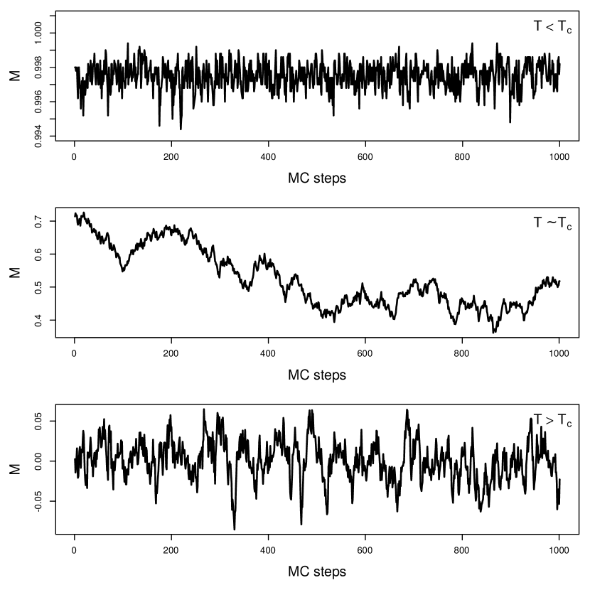
Fig. 1 shows the time series at three regimes $T<T_{c}$, $T\simeq T_{c}$, and $T>T_{c}$ from top to bottom respectively. Obviously we can observe different outlines of the time series at different temperature regimes. Detailed properties of those time series will be analyzed by using multifractal detrended analysis and visibility graph method in the following context.

Figure 2: First four moments of the magnetization time series. Ensemble average of (a) mean, (b) variance, (c) skewness (d) kurtosis of the magnetization time series versus the relative temperature, $T/T_{c}$ for system size $N=100\times 100$.

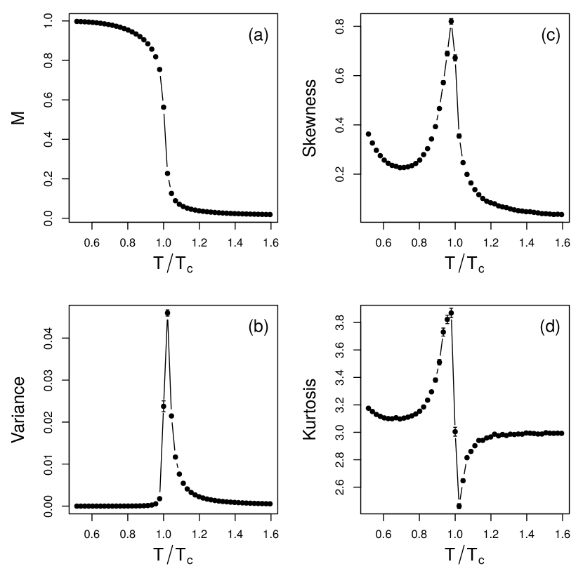
The trends of magnetization time series at different temperature are obviously different. We use first four order moments to quantify the distribution differences between those time series in Fig. 2. The ensemble standard errors are defined as standard deviation divided by square root of ensemble size (100) and are shown with error bars in figures. Fig. 2 (a) is the ensemble average magnetization vary with relative temperature $T/T_{c}$. Simulation results have confirmed the existence of phase transition around theoretical critical temperature $T_{c}\simeq 2.27$. This transition can also be verified from three statistical quantities in Fig. 2 : (b) variance, (c) skewness and (d) kurtosis which have been fully discussed in Ref[36]. Those moments have been used as early warnings of phase transition therein. The variance is almost zero at non-critical regimes, but it becomes relatively large around critical point. The abrupt change at low temperature regime is obviously different from the continuous evolution at high temperature regime. Thus the variance can not be recognized as a useful early warning when reaching the system from low temperature regime. Skewness is related to the asymmetry of events in the time series. It is large only in the low temperature regime and reaches its maxima at critical point and it becomes very small at high temperature regime. This is due to the meta-stable states at low temperature[36]. The stochastic permutation is not strong enough to make the system escape from the meta-stable states. This makes the distribution of magnetization asymmetric. The kurtosis fluctuates severely around critical point and becomes very close to the reference normal distribution (which has a kurtosis equal to 3) when $T\ll T_{c}$ and $T\gg T_{c}$. Apparent distribution differences between magnetization time series at different temperature regimes give a hint about the structure heterogeneous which demands more detailed investigations.

MF-DFA

If we set $q=2$ in the MF-DFA, we get the same results as standard DFA method. The Hurst exponents $h(q=2)$ have been used as early warning to detect the rising memory in time series of a system close to critical point[30, 9]. We have calculated the ensemble average of Hurst exponent $h(q=2)$ in Fig. 3. The Hurst exponent $h(q=2)\simeq 0.5$ when $T\ll T_{c}$ and $T\gg T_{c}$ which means the magnetization time series are short range correlated at these two regimes. When $T\sim T_{c}$ the Hurst exponent increases rapidly which results in $h(q=2)>1$. This means the time series becomes non-stationary which turns to be a unbounded process. The Hurst exponent $h(q=2)\geq 1.2$ when temperature gets very close to critical temperature. This indicates that the magnetization time series posses long range correlation when the system approaches critical regime. The Hurst exponent behave almost the same when we use different system size.

Figure 3: Hurst exponent at different temperature. (Color online) Ensemble average of the Hurst exponent $h(q=2)$ versus the relative temperature $T/T_{c}$ for different system sizes.

Figure 4: Generalized Hurst exponent at different temperature. (Color online) Heat map of ensemble average of the generalized Hurst exponent $h(q)$ for $q\in[-5,5]$ at different temperature regimes for different system sizes.

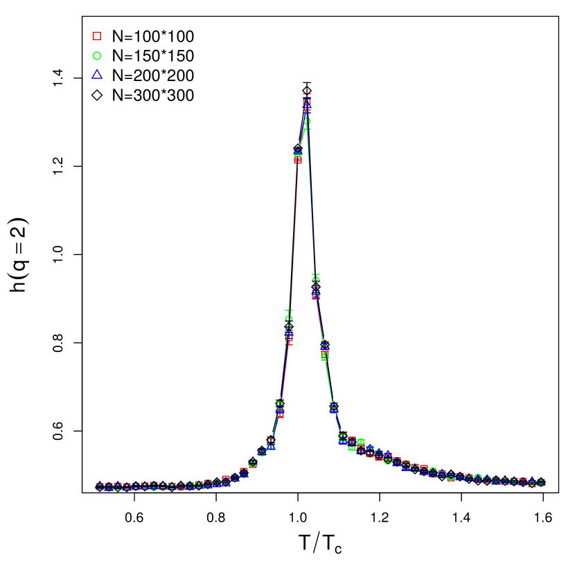
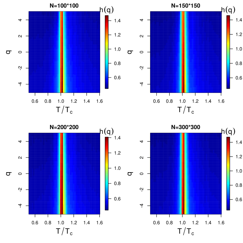
Fig. 4 shows the generalized Hurst exponents $h(q)$ at different temperatures for $q\in[-5,5]$ with $\Delta_{q}=0.1$. The system sizes are $N=100\times 100,150\times 150,200\times 200,300\times 300$. When $T\ll T_{c}$ and $T\gg T_{c}$ the weak dependence on $q$ of $h(q)$ show the weak multifractal (monofractal) structures of time series. As the system approaches the critical regime, $h(q)$ become strongly depend on $q$. The small and large fluctuations of the Ising system near critical point display different scaling behaviours. The strong non-linear dependence on $q$ of $h(q)$ around $T_{c}$ reveals the strong mutifractal nature of the Ising system in the time domain. Transformation of the multifractal properties uncover the apparent structural and dynamical differences of the Ising system at different temperature regimes.

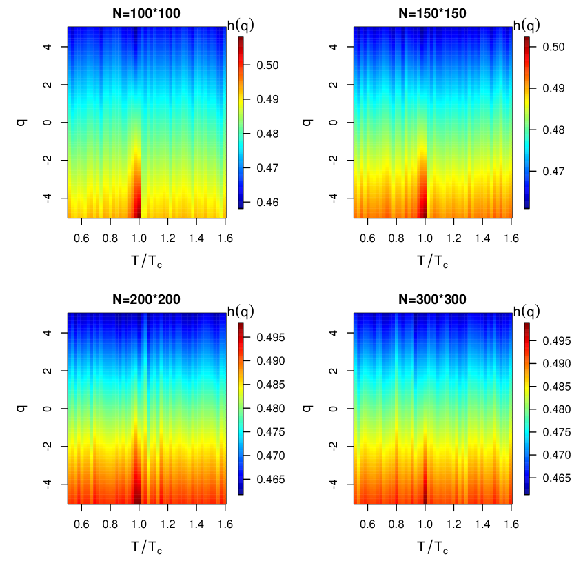
Heat map of $h(q)$ for different $q$ at different temperatures presented in Fig. 4 has given a comprehensive description about scaling behaviours of the fluctuations at different magnitude. Dramatic increase of the generalized Hurst exponent around critical temperature at different order $q$, not only at $q=2$, can be observed. We can see that the generalized Hurst exponent is very close to 0.5 and then it becomes remarkably larger than 1 around critical point at all observed order $q\in[-5,5]$. This indicates that the generalized Hurst exponent is also a very good indicator of phase transition. Multifractality of the time series increase remarkably around critical point. Those characteristics should also be very good early warnings[36, 44].

Figure 5: Singularity spectrum at different temperature regimes. (Color online) Singularity spectrum $f(\alpha)$ of the time series as a function of the singularity strength $\alpha$ at different temperature regimes for different system sizes.

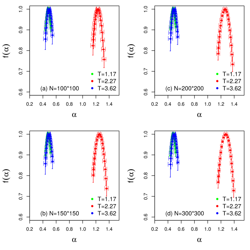
In order to quantify the level of mulfitracality, the singularity spectrum of the time series at different temperatures for different system sizes have been presented in Fig. 5. The maximum of the $\alpha_{0}$ increases to 1.3 when $T\sim T_{c}(2.27)$, but it decreases to 0.5 when temperature deviates form $T_{c}$. We can observe that the width of singularity spectrum increases as $T$ approaches $T_{c}$. At the same instant the singularity becomes right skew. Those changes indicate more complex time series around critical temperature. The evolution of the singularity spectrum at different temperatures are basic consistent for different system sizes.

A more quantitative measure about the level of complexity of the series can be given by fitting the singularity spectrum[48] and calculating the multifractal spectrum parameters: position of maximum $\alpha_{0}$; width of the spectrum $W=\alpha_{max}-\alpha_{min}$; and the skew parameter $r=(\alpha_{max}-\alpha_{0})/(\alpha_{0}-\alpha_{min})$ as described in previous method section. A large value of $\alpha_{0}$ suggests the time series is irregular. Larger value of $W$ means richer structure of the series. Meanwhile the skew parameter $r$ determines which fractal exponents are dominant. These parameters lead to a comprehensive measure of the singularity complexity of the time series: a series with large value of $\alpha_{0}$, a wide range $W$ of fractal exponents, and a right-skewed shape may be considered more complex than one with opposite characteristics[45].

Figure 6: Complexity measure of the singularity spectrum and autocorrelation length of time series. (Color online) The complexity measure of the time series at different temperature: (a) the position of maximum $\alpha_{0}$, (b) the width of the spectrum $W$, (c) the skew parameter $r$ for different system size, (d) critical length of the autocorrelation length $S_{c}$ for different system sizes.

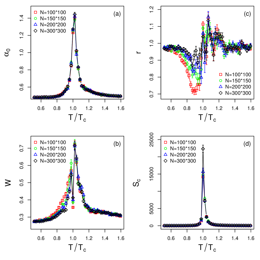
As shown in Fig. 6 (a) the value of $\alpha_{0}$ becomes very large at $T\sim T_{c}$ which suggests that the series become extremely irregular. The evolution pattern of $\alpha_{0}$ can serve as a very good early warning about the coming of the critical transition. The increase of the width $W$ of the spectrum in Fig. 6 (b) indicates richer structure near critical regime. The abrupt jump right at the critical point gives a hint about the mutation of the correlation structure. The skew parameters $r$ in Fig. 6 (c) are almost equal to 1 when temperature deviates from critical regime which manifest symmetry shapes of the multifractal spectrum at low and high temperature regimes. It becomes larger than 1 at critical threshold. One interesting finding is that the skew parameter $r$ first gradually decreases at lower temperature regime and it increases very fast when the system gets particularly close to critical temperature. This shows that the large fluctuations dominate when the system approaches critical regime from the lower temperature. On the contrary the skew parameter $r$ will slowly increase to the maxima when the system moving close to $T_{c}$ from the right side. Thus the small fluctuations contribute the most to the multifractality at critical point. This indicates a more complex structure with right skewed shape above the critical regime.

Figure 7: Generalized Hurst exponent for shuffled time series. (Color online) Heat map of ensemble average of the generalized Hurst exponents $h(q)$ for $q\in[-5,5]$ at different temperature regimes for the shuffled time series.

Figure 8: Singularity spectrum for shuffled time series. (Color online) Singularity spectrum of the original time series and the singularity spectrum of the shuffled time series.

There are two main sources of multifracality which we would like to distinguish[22, 58]: (i) Multifractality due to broad probability density function. (ii) Multifractality due to different long-term correlations of small and large fluctuations. Fig. 6 (d) gives the critical length of the autocorrelation as a function of relative temperature. The critical length of the autocorrelation function is the maximum lag at which the autocorrelation smaller than the critical value $2/\sqrt{l}$. According to a recent research about the DFA on auto regression process (AR(1)), the autocorrelation length can be used to help estimating the Hurst exponent more accurately[34]. It is known that the two point correlation function of Ising system will become divergence in the thermodynamic limit (large N) at critical point. The divergence of two point correlation makes the autocorrelation of the magnetization time series divergent. Thus the strong multifractality of the Ising system around critical point should at least caused in part by the divergence of autocorrelation.

Here we proceed the same analysis as in Fig. 4 and 5, but shuffling the data randomly to better identify the source of multifractality. Multifractality caused by broad probability density function can not be fully eliminated by the shuffling procedure. Meanwhile multifractality induced by long-term correlations can be removed after shuffling the time series. The shuffling procedures have been performed $1000\times l$ transpositions on each series with 100 ensemble average. While $l=100000$ is the length of each time series. Fig. 7 gives the dependency between $h(q)$ and $q$ for the shuffled time series at different temperature under different system sizes. The strong non-linear dependency only exist when $T\sim T_{c}$. 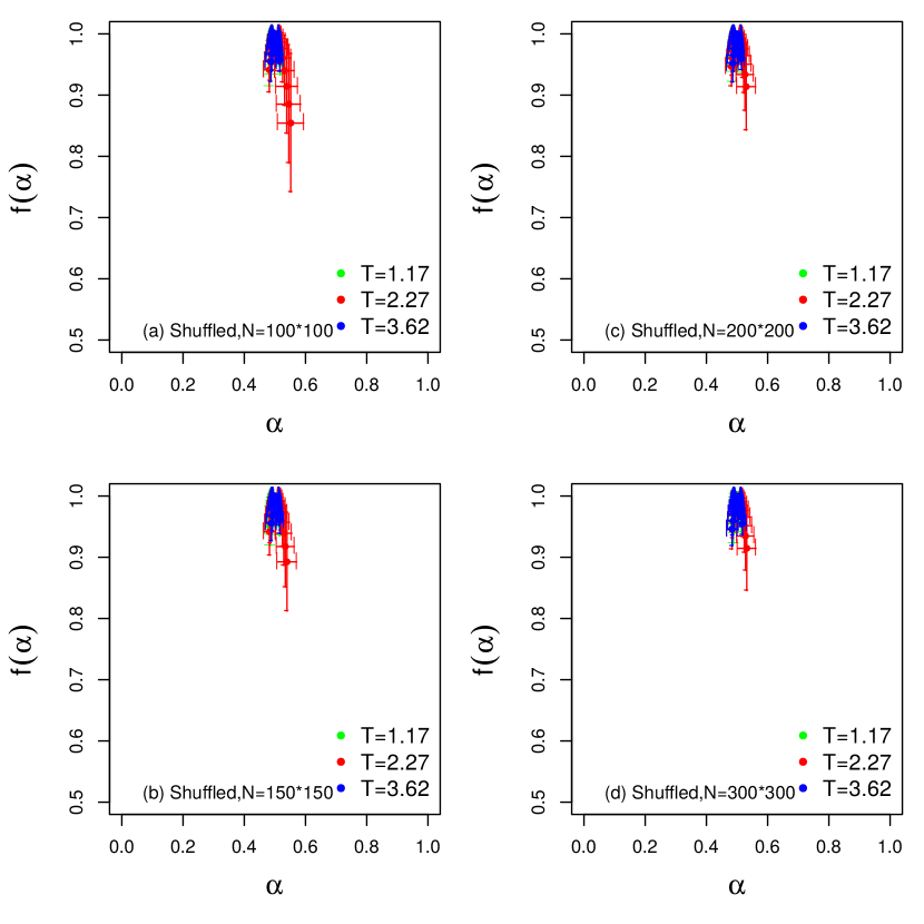In Fig. 8 we show the singularity spectrum of shuffled time series at three temperature regimes for different system sizes. We find that the singularity spectrum at $T=1.17$ and $T=3.62$ are nearly at one point with $\alpha_{0}\simeq 0.5$. On the contrary the singularity spectrum of the time series at $T=2.27$ still posses multifractality with a right skew shape. We address that the source of strong multifractality of the system near critical regime stems from both long-term correlations and broad probability density function[5].

Visibility Graph

We use the visibility graph method to convert magnetization time series under different temperatures to complex networks. The networks’ sizes are 10000 which converted from time series with length 10000. Then different topological quantities have been calculated for networks obtained at different temperatures. Those topology quantities[1] can characterize the geometrical properties of time series which are directly related to the dynamics of Ising system.

Figure 9: Visibility graphs at different temperature regimes. (Color online) The network structure of the visibility graphs at (a) $T=1.17$, (b) $T=2.27$, (c) $T=3.62$. The network sizes are 10000. Different colors represent different communities.

Here we give three networks obtained via visibility graph method from three different time series at three different temperatures in Fig. 9. Fig. 9(a), (b), (c) are the visibility graphs at $T=1.17,2.27,3.62$ respectively. The network at $T=2.27$ is markedly different from two networks at $T=1.17,3.62$. The extremely modular network structure is exhibited in Fig. 9(b). It can be understood that when $T=2.27$ the large trends of the time series make some extreme values have massive visibilities. This is responsible for the formation of large communities which presented by different colors. Two networks in Fig.9(a) and (c) possess tree like structures. The community sizes of these two networks are small than the network when $T=2.27$. The lack of trends leads to the snowflake shapes. Thus the geometric outlines of the time series at different temperature regimes are preserved due to the affine invariant features of the visibility graph method.

Figure 10: Cumulative degree distributions of visibility graphs. Cumulative degree distributions of networks at three different temperature regimes with (a) $T=1.17$, (b) $T=2.27(T_{c})$, (c) $T=3.62$ respectively for system size $N=100\times 100$.

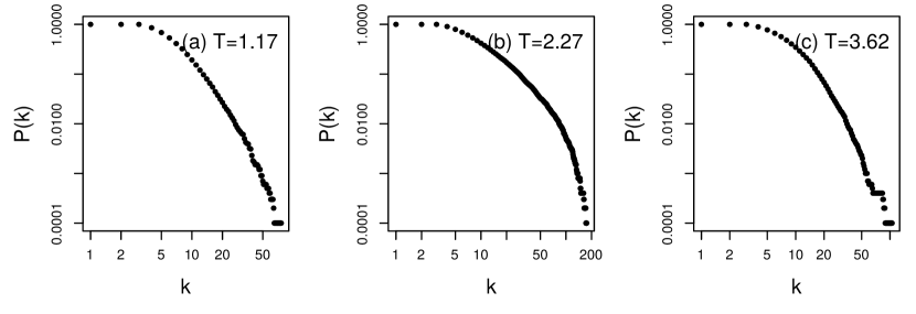
Fig. 10 gives the degree distributions of networks at three temperature regimes. Fig.  10 (a), (b), (c) are degree distributions of networks at temperature $T=1.17$, $T=2.27(T_{c})$ and $T=3.62$ respectively. Three distributions show the heterogeneous nature of the networks at three temperature regimes. The network at $T=T_{c}$ with broader degree distribution is apparently more heterogeneous than those at $T<T_{c}$ and $T>T_{c}$. The largest degree of network at $T=T_{c}$ is 288 which is significantly larger than those networks’ largest degree away from critical temperature. This can also be verified in Fig.  11 (f): heterogeneity[12] of the networks increase dramatically near critical point. According to Ref[29], fractal time series will be converted to scale-free network. So from the degree distributions of networks we can gain some insights about the fractal nature of magnetization time series which has been discussed by using MF-DFA.

Figure 11: Topology quantities of visibility graphs. (Color online) Ensemble average of the topology quantities (a) clustering coefficient $C$ , (b) average degree $K$, (c) average shortest path length $L$, (d) the density $D$, (e) the assortativity $A$, (f) the heterogeneity $H$ of networks converted from time series at different temperature. Different colors and symbols represent different system sizes.

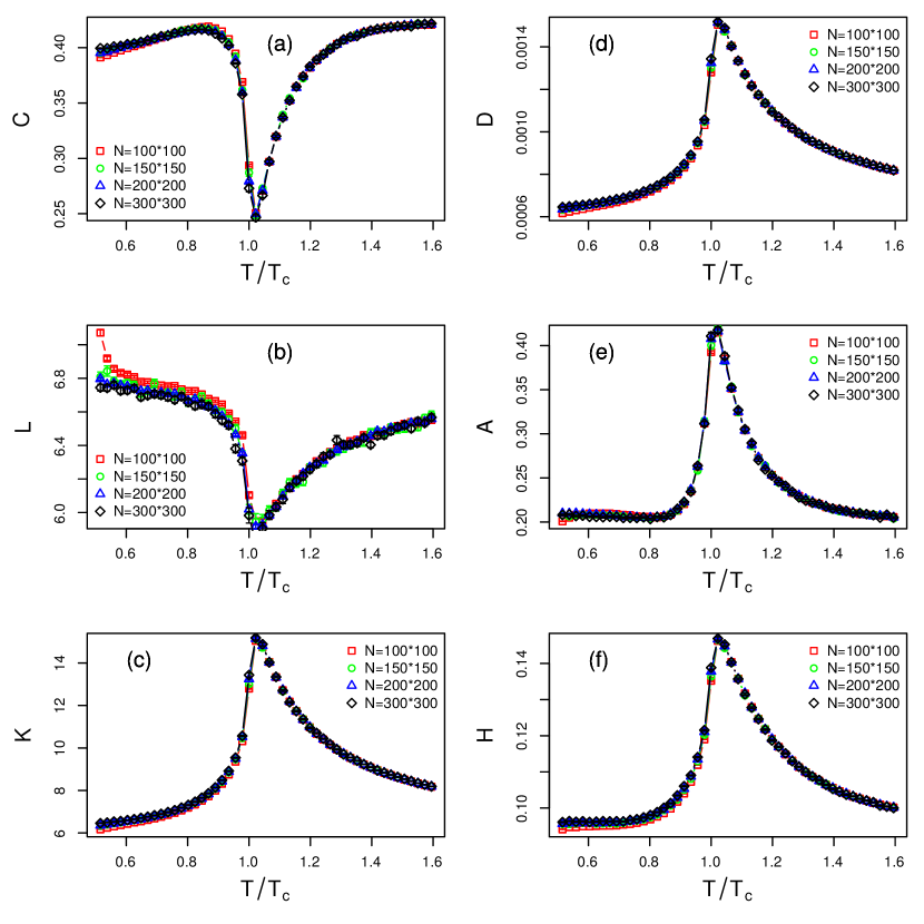
In Fig. 10, networks at different regimes share the heterogeneous nature, but they do have some differences which are related to the dynamic properties of Ising system at specific temperature. In Fig.  11, we calculate the ensemble average of topology quantities at different temperature. In Fig.  11 (a), the clustering coefficient $C$, (b) average shortest path length $L$ both decrease around the critical point. Decreases of $C$ and $L$ around critical point indicate more heterogeneous network structures. We can verify these changes from Fig.  11 (f). According to Ref[12], heterogeneity of the BA network[3] is around 0.11 which is much smaller than the heterogeneity of network at critical point. The extreme heterogeneous structure is due to utmost non-stationarity and long-term correlations of the time series which is exactly the characterizations of critical state of Ising system. The average degree $K$, network density $D$ in Fig.  11 (c) and (d) reach their maxima around critical temperature. The network becomes more and more dense when the system approaches $T_{c}$. Fig.  11 (e) shows the assortativity $A$ as a function of relative temperature. The fast increase of $A$ around $T_{c}$ gives a hint about the coming of the critical threshold. It also tells that the network becomes more and more assortative which means the existence of long trends and extreme values in the time series near $T_{c}$. All those topology quantities transitions suggest huge structure distinctions between networks at different temperature regimes. Those results have shown geometrical structure transition of the time series at different regimes which are signals of phase transition of Ising system from the view of complex networks. The way of those topological quantities approach the critical point either form the low temperature side or the high temperature side have manifest the possibility of been used as early warnings.

As a final remark of the paper, we shall emphasize the importance of our previous results from the view of early warnings[44, 25, 36]. Variety of early warning signals have been proposed and summarized [44, 9, 13, 36]. Those early warnings can be categorized into two main classes: metric-based indicators which probing the delicate changes in the statistical properties of the time series, and model-based indicators which detect changes in the time series dynamic fitted by a reasonable model. Thus our results shown in previous sections are metric-based estimators. The four order moments given in Fig. 2 has been fully discussed in ref [36]. It is exactly consistent with previous researches that the critical slowing down and the fluctuation patterns of the complex system near critical thresholds will make the autocorrelation, variance and skewness increase[19, 16, 31]. The contribution of our work is that the MF-DFA and visibility graph elaborate the multifractal and geometrical properties of the Ising system near critical point in the time domain. So far as we know this is the first time to use the variation of the multifractal and geometrical properties of the system as early warnings. In fact due to the divergence of the spatial correlation of Ising system near critical threshold, the spatial multifractal features may also be used as early warning signals. We can use the higher dimension MF-DFA[14, 7, 59] to explore this problem. This should be subject to future investigations.

Conclusions

In conclusion, we have used the mutifractal detrended analysis (MF-DFA) and the visibility graph method to analyze the outputs of two-dimensional Ising model - magnetization time series. Dynamics of the system at different temperatures are directly related to the multifractal and geometrical properties of time series. First four order statistical moments confirmed the existence of phase transition around theoretical critical temperature. The variance, skewness and kurtosis have been shown as three very efficient early warnings as discussed in recent Ref[36]. According to the MF-DFA, classical Hurst exponent $h(q=2)$ shows the extreme non-stationarity of magnetization time series at critical temperature. Also the generalized Hurst exponents uncover the transformation of time series form weak multifractal(monofractal) to strong multifractal when temperature approaches to critical regime. This indicates that the generalized Hurst exponent is a good indicator of phase transition along with statistical moments. The singularity spectrum and the complexity parameters have been employed to inspect multifractality level of magnetization time series at different temperatures. The shape of singularity spectrum around critical point becomes very complicated which depict the complex dynamics of Ising system. The evolution of the complexity parameters show the strong multifractality of the system at critical regime quantitatively. The shuffling procedure has identified the sources of multifractality of the system near critical point stem both from broad probability density function and long-term correlations. The visibility graph method has been employed to convert the magnetization time series to complex networks. Heterogeneous degree distributions of the complex networks at three temperature regimes have shown the fractal nature of magnetization time series. Basic topological quantities of networks can capture the geometrical variation of time series. The decreases and increases of those topological quantities near critical regime have manifested the critical dynamics of Ising system. Those evolution patterns can help us identifying how far the system is away form critical point. Thus we then conclude that the generalized Hurst exponent, the level of multifractality and the topological quantities of visibility graphs can serve as early warnings for diverse of complex systems. The MF-DFA and the visibility graph method may not only be limited here for the analysis of two-dimensional Ising system, but can be used as powerful tools to analyze the critical behaviours of many other systems. Thus we propose that the multifractality and complex network topological quantities can be used as early warnings for various complex systems near critical thresholds.

References

- 1. Réka Albert and Albert Laszlo Barabasi. Statistical mechanics of complex networks. Reviews of Modern Physics, 74(1):47–97, 2002.
- 2. Miroslav Andjelkovi, Neelima Gupte, and Bosiljka Tadi. Hidden geometry of traffic jamming. PHYSICAL REVIEW E, 91:1–8, 2015.
- 3. Albert-Laszlo Barabasi and Reka Albert. Emergence of scaling in random networks. Science, 286(October):11, 1999.
- 4. Albert Lszl Barabsi and Tams Vicsek. Multifractality of self-affine fractals. Physical Review A, 44:2730–2733, 1991.
- 5. Jozef Barunik, Tomaso Aste, T. Di Matteo, and Ruipeng Liu. Understanding the source of multifractality in financial markets. Physica A: Statistical Mechanics and its Applications, 391(17):4234–4251, 2012.
- 6. Stephen G. Brush. History of the Lenz-Ising model. Reviews of Modern Physics, 39(4):883–893, 1967.
- 7. Anna Carbone. Algorithm to estimate the Hurst exponent of high-dimensional fractals. Physical Review E - Statistical, Nonlinear, and Soft Matter Physics, 76(5):1–7, 2007.
- 8. Claudio Castellano, Santo Fortunato, and Vittorio Loreto. Statistical physics of social dynamics. Reviews of Modern Physics, 81(2):591–646, may 2009.
- 9. Vasilis Dakos, Stephen R. Carpenter, William A. Brock, Aaron M. Ellison, Vishwesha Guttal, Anthony R. Ives, Sonia Kéfi, Valerie Livina, David A. Seekell, Egbert H. van Nes, and Marten Scheffer. Methods for Detecting Early Warnings of Critical Transitions in Time Series Illustrated Using Simulated Ecological Data. PLoS ONE, 7(7):e41010, 2012.
- 10. Paulo Duarte-Neto, Borko Stošić, Tatijana Stošić, Rosangela Lessa, Milorad V. Milošević, and H. Eugene Stanley. Multifractal Properties of a Closed Contour: A Peek beyond the Shape Analysis. PLoS ONE, 9(12):e115262, 2014.
- 11. Srimonti Dutta. Multifractal properties of ECG patterns of patients suffering from congestive heart failure, 2010.
- 12. Ernesto Estrada. Quantifying network heterogeneity. Physical Review E, 82(6):66102, 2010.
- 13. Davide Faranda, Bérengère Dubrulle, and Flavio Maria Emanuele Pons. Statistical early-warning indicators based on autoregressive moving-average models. Journal of Physics A: Mathematical and Theoretical, 47(25):252001, 2014.
- 14. Gao Feng Gu and Wei Xing Zhou. Detrended fluctuation analysis for fractals and multifractals in higher dimensions. Physical Review E - Statistical, Nonlinear, and Soft Matter Physics, 74(6):1–13, dec 2006.
- 15. Gao-Feng Gu and Wei-Xing Zhou. Detrending moving average algorithm for multifractals. Physical Review E, 82(1):011136, jul 2010.
- 16. Vishwesha Guttal and Ciriyam Jayaprakash. Changing skewness: an early warning signal of regime shifts in ecosystems. Ecology Letters, 11(5):450–460, 2008.
- 17. Rashid Hasan and Salim M. Mohammad. Multifractal analysis of Asian markets during 2007–2008 financial crisis. Physica A: Statistical Mechanics and its Applications, 419:746–761, feb 2015.
- 18. Ernst Ising. Beitrag zur theorie des ferromagnetismus. Zeitschrift fur Physik, 31(1):253–258, 1925.
- 19. Anthony R Ives, Ecological Monographs, No May, and R Ives. Measuring Resilience in Stochastic Systems MEASURING RESILIENCE IN STOCHASTIC SYSTEMS ’. Ecological Monographs, 65(2):217–233, 1995.
- 20. Zhi-Qiang Jiang and Wei-Xing Zhou. Multifractal analysis of Chinese stock volatilities based on the partition function approach. Physica A: Statistical Mechanics and its Applications, 387(19-20):4881–4888, aug 2008.
- 21. Zhi-Qiang Jiang and Wei-Xing Zhou. Multifractal detrending moving-average cross-correlation analysis. Physical Review E, 84(1):016106, jul 2011.
- 22. Jan W. Kantelhardt. Fractal and Multifractal Time Series. page 59, 2008.
- 23. Jan W Kantelhardt, Eva Koscielny-Bunde, Henio H.a Rego, Shlomo Havlin, and Armin Bunde. Detecting long-range correlations with detrended fluctuation analysis. Physica A: Statistical Mechanics and its Applications, 295:441–454, 2001.
- 24. Jan W. Kantelhardt, Stephan a. Zschiegner, and H. Eugene Stanley. Multifractal detrended uctuation analysis of nonstationary time series. Physica A, 316:87–114, 2002.
- 25. Sonia Kéfi, Vishwesha Guttal, William a. Brock, Stephen R. Carpenter, Aaron M. Ellison, Valerie N. Livina, David a. Seekell, Marten Scheffer, Egbert H. Van Nes, and Vasilis Dakos. Early warning signals of ecological transitions: Methods for spatial patterns. PLoS ONE, 9(3):10–13, 2014.
- 26. LADISLAV KRISTOUFEK. FRACTAL MARKETS HYPOTHESIS AND THE GLOBAL FINANCIAL CRISIS: SCALING, INVESTMENT HORIZONS AND LIQUIDITY. Advances in Complex Systems, 15(06):1250065, 2012.
- 27. Jarosław Kwapień and Stanisław Drożdż. Physical approach to complex systems. Physics Reports, 515(3-4):115–226, jun 2012.
- 28. L. Lacasa, B. Luque, J. Luque, and J. C. Nuño. The visibility graph: A new method for estimating the Hurst exponent of fractional Brownian motion. EPL (Europhysics Letters), 86(3):30001, may 2009.
- 29. Lucas Lacasa, Bartolo Luque, Fernando Ballesteros, Jordi Luque, and Juan Carlos Nuño. From time series to complex networks: the visibility graph. Proceedings of the National Academy of Sciences of the United States of America, 105(13):4972–5, apr 2008.
- 30. E. Landa, Irving O. Morales, R. Fossion, P. Stránský, V. Velázquez, J. C. López Vieyra, and A. Frank. Criticality and long-range correlations in time series in classical and quantum systems. Physical Review E - Statistical, Nonlinear, and Soft Matter Physics, 84(1):1–5, 2011.
- 31. Timothy M Lenton, Richard J Myerscough, Robert Marsh, Valerie N Livina, Andrew R Price, Simon J Cox, and Genie Team. Using GENIE to study a tipping point in the climate system. Philosophical transactions. Series A, Mathematical, physical, and engineering sciences, 367(1890):871–884, 2009.
- 32. Chuang Liu, Wei-Xing Zhou, and Wei-Kang Yuan. Statistical properties of visibility graph of energy dissipation rates in three-dimensional fully developed turbulence. Physica A: Statistical Mechanics and its Applications, 389(13):2675–2681, jul 2010.
- 33. Benoit B. Mandelbrot. The Fractal Geometry of Nature, 1983.
- 34. H Marc and Holger Kantz. The fluctuation function of the detrended fluctuation analysis - Investigation on the AR ( 1 ) process. European Physical Journal B, (1):1–15, 2015.
- 35. Nicholas Metropolis, Arianna W. Rosenbluth, Marshall N. Rosenbluth, Augusta H. Teller, and Edward Teller. Equation of State Calculations by Fast Computing Machines. The Journal of Chemical Physics, 21(6):1087–1092, 1953.
- 36. Irving O. Morales, Emmanuel Landa, Carlos Calderon Angeles, Juan C. Toledo, Ana Leonor Rivera, Joel Mendoza Temis, and Alejandro Frank. Behavior of Early Warnings near the Critical Temperature in the Two-Dimensional Ising Model. Plos One, 10(6):e0130751, 2015.
- 37. Raffaello Morales, T. Di Matteo, and Tomaso Aste. Non-stationary multifractality in stock returns. Physica A: Statistical Mechanics and its Applications, 392(24):6470–6483, 2013.
- 38. Raffaello Morales, T. Di Matteo, Ruggero Gramatica, and Tomaso Aste. Dynamical generalized Hurst exponent as a tool to monitor unstable periods in financial time series. Physica A: Statistical Mechanics and its Applications, 391(11):3180–3189, 2012.
- 39. M E J Newman, D J Watts, and S H Strogatz. Random graph models of social networks. PNAS, 99 Suppl 1:2566–72, 2002.
- 40. G. Oh, C. Eom, S. Havlin, W. S. Jung, F. Wang, H. E. Stanley, and S. Kim. A multifractal analysis of Asian foreign exchange markets. The European Physical Journal B, 85(6):0–6, 2012.
- 41. C. K. Peng, S. V. Buldyrev, S. Havlin, M. Simons, H. E. Stanley, and a. L. Goldberger. Mosaic organization of DNA nucleotides. Physical Review E, 49(2):1685–1689, 1994.
- 42. Boris Podobnik and H. Stanley. Detrended Cross-Correlation Analysis: A New Method for Analyzing Two Nonstationary Time Series. Physical Review Letters, 100(8):084102, feb 2008.
- 43. Yong Ping Ruan and Wei Xing Zhou. Long-term correlations and multifractal nature in the intertrade durations of a liquid Chinese stock and its warrant. Physica A: Statistical Mechanics and its Applications, 390(9):1646–1654, 2011.
- 44. Marten Scheffer, Jordi Bascompte, William A. Brock, Victor Brovkin, Stephen R. Carpenter, Vasilis Dakos, Hermann Held, Egbert H. van Nes, Max Rietkerk, and George Sugihara. Early-warning signals for critical transitions. Nature, 461(7260):53–59, 2009.
- 45. YU SHIMIZU, STEFAN THURNER, and KLAUS EHRENBERGER. Multifractal spectra as a measure of complexity in human posture. Fractals, 10(01):103–116, 2002.
- 46. FM Siokis. Multifractal analysis of stock exchange crashes. Physica A: Statistical Mechanics and its Applications, 392(5):1164–1171, 2013.
- 47. Didier Sornette. Physics and financial economics (1776-2014): puzzles, Ising and agent-based models. Reports on progress in physics. Physical Society (Great Britain), 77(6):062001, jun 2014.
- 48. Darko Stošić, Dusan Stošić, Tatijana Stošić, and H Eugene Stanley. Multifractal analysis of managed and independent float exchange rates. Physica A: Statistical Mechanics and its Applications, 428:13–18, 2015.
- 49. Dusan Stošić, Darko Stošić, Tatijana Stošić, and H. Eugene Stanley. Multifractal properties of price change and volume change of stock market indices. Physica A: Statistical Mechanics and its Applications, 428:46–51, 2015.
- 50. Luciano Telesca and Vincenzo Lapenna. Measuring multifractality in seismic sequences. Tectonophysics, 423(1-4):115–123, 2006.
- 51. Marco Thiel, M. Carmen Romano, and Jürgen Kurths. How much information is contained in a recurrence plot? Physics Letters, Section A: General, Atomic and Solid State Physics, 330(5):343–349, 2004.
- 52. Xiaoke Xu, Jie Zhang, and Michael Small. Superfamily phenomena and motifs of networks induced from time series. Proceedings of the National Academy of Sciences of the United States of America, 105(50):19601–19605, 2008.
- 53. Yue Yang, Jianbo Wang, Huijie Yang, and Jingshi Mang. Visibility graph approach to exchange rate series. Physica A: Statistical Mechanics and its Applications, 388(20):4431–4437, oct 2009.
- 54. Yue Yang and Huijie Yang. Complex network-based time series analysis. Physica A: Statistical Mechanics and its Applications, 387(5-6):1381–1386, feb 2008.
- 55. J. Zhang and M. Small. Complex Network from Pseudoperiodic Time Series: Topology versus Dynamics. Physical Review Letters, 96(23):238701, jun 2006.
- 56. Yi Zhao, Tongfeng Weng, and Shengkui Ye. Geometrical invariability of transformation between a time series and a complex network. Physical Review E, 90(1):012804, jul 2014.
- 57. Wei-Xing Zhou. Multifractal detrended cross-correlation analysis for two nonstationary signals. Physical Review E, 77(6):066211, jun 2008.
- 58. Wei Xing Zhou. Finite-size effect and the components of multifractality in financial volatility. Chaos, Solitons and Fractals, 45(2):147–155, 2012.
- 59. Yu Zhou, Yee Leung, and Zu Guo Yu. Relationships of exponents in two-dimensional multifractal detrended fluctuation analysis. Physical Review E - Statistical, Nonlinear, and Soft Matter Physics, 87(1):4–7, 2013.
- 60. Todd Zorick and Mark A. Mandelkern. Multifractal Detrended Fluctuation Analysis of Human EEG: Preliminary Investigation and Comparison with the Wavelet Transform Modulus Maxima Technique. PLoS ONE, 8(7):e68360, 2013.