Quantum machine learning with glow for episodic tasks and decision games

Abstract

We consider a general class of models, where a reinforcement learning (RL) agent learns from cyclic interactions with an external environment via classical signals. Perceptual inputs are encoded as quantum states, which are subsequently transformed by a quantum channel representing the agent’s memory, while the outcomes of measurements performed at the channel’s output determine the agent’s actions. The learning takes place via stepwise modifications of the channel properties. They are described by an update rule that is inspired by the projective simulation (PS) model and equipped with a glow mechanism that allows for a backpropagation of policy changes, analogous to the eligibility traces in RL and edge glow in PS. In this way, the model combines features of PS with the ability for generalization, offered by its physical embodiment as a quantum system. We apply the agent to various setups of an invasion game and a grid world, which serve as elementary model tasks allowing a direct comparison with a basic classical PS agent.

I Introduction

I.1 Motivation

If we consider the development of new technologies as a collective learning process, we can distinguish between different interlaced processes. While basic research focuses on exploration characterised by a search for potential alternatives to established methods, the more promising an approach appears, the more likely it becomes subject to subsequent exploitation, where it is optimised and matured with the ultimate hope to supersede what is available. An example of explorative activity are early efforts to solve problems by artificial intelligence (AI), such as inventing unconventional heuristic techniques. AI has recently regained interest Nature (2015); Science (2015), which may be a consequence of new approaches to computation Nielsen and Chuang (2000); Wittek (2014) as well as improved capacities of classical computing and networking. The present work aims at drawing a connection between the recently suggested scheme of PS Briegel and las Cuevas (2012); Mautner et al. (2015) and quantum control theory D’Alessandro (2008); Wiseman and Milburn (2009), restricting attention to example problems analogous to those considered in the basic classical PS schemes Briegel and las Cuevas (2012); Mautner et al. (2015); Melnikov et al. (2014, 2015), rather than a treatment of practically relevant but large-scale applications of, e.g., machine learning. A discussion of scalability, quantum speed up, or practical implementability Paparo et al. (2014); Dunjko et al. (2015); Friis et al. (2015) is beyond the scope of this work.

We consider a class of schemes, where a quantum agent learns from cyclic interactions with an external environment via classical signals. The learning can be considered as an internal quantum navigation process of the agent’s “hardware” or “substrate” that forms its memory of past experience. For notational convenience, we describe the memory operation as a unitary $\hat{U}$ involving (information carrying and other) controllable and uncontrollable degrees of freedom (such as a “bath”), where the latter are not necessarily identical with the environment, on which the agent operates. While conceptually, the memory may hence be seen as an open quantum system Breuer and Petruccione (2002), the numerical examples considered in the present work restrict to closed system dynamics. This navigation of agent memory $\hat{U}$ must be distinguished from the evolution of quantum states in which, following external or internal stimulus, the memory is excited Briegel and las Cuevas (2012); Paparo et al. (2014). Learning as an internal navigation process corresponds to the colloquial notion of a learner desiring to quickly “make progress” rather than “marking time”. For the agent’s internal dynamics, we talk of a navigation process rather than a navigation problem that is to be solved, since ultimately, the agent responds to its environment that is generally unknown and subject to unpredictable changes.

While the proposed PS-model is characterised by an episodic & compositional memory (ECM), we here ignore the clip network aspect and restrict attention to a parameter updating that is motivated from the basic scheme Briegel and las Cuevas (2012); Mautner et al. (2015), which we apply to simple learning tasks involving an agent equipped with a quantum memory. We specifically reconsider some of the examples discussed in Briegel and las Cuevas (2012); Melnikov et al. (2014, 2015) in order to investigate to what extent the results can be reproduced. In contrast to the classical scheme, where the parameters are weights in a clip network, we here refrain from ascribing a particular role, they could play (e.g., in a quantum walk picture mentioned in Briegel and las Cuevas (2012)). Here, the parameters are simply controls, although in our examples, they are defined as interaction strengths in a stack of layers constituting the agent memory $\hat{U}$. This choice of construction is however not essential for the main principle. From the viewpoint of the network-based classical PS, drawing a connection to quantum control theory opens the possibility to apply results obtained in the latter field over the last years Dong et al. (2006a); *Dong06b; *Dong08a; *Dong08b; *Dong09; *Dong10; *Dong14; *Dong15. On the other hand, classical PS is similar to RL Sutton and Barto (1998); Russell and Norvig (2009), which considers a type of problems, where an “agent” (embodied decision maker or “controller”) learns from interaction with an environment (controlled system or “plant”) to achieve a goal. The learning consists in developing a (generally stochastic) rule, the agent’s “policy”, of how to act depending on the situation it faces, with the goal to accumulate “reward” granted by the environment. In RL, the environment is anything outside of control of this decision making. The reward could describe for example pleasure or pain felt by an individual. It is generated within the individual’s body but is beyond it’s control, and therefore considered originating in the agent’s environment. Historically, RL, which must be distinguished from supervised learning, originates from merging a trait in animal psychology with a trait in control theory. Although dynamic programming as the basis of the latter is well understood, limited knowledge of the environment along with a vast number of conceivable situations, an RL-agent may face, render a direct solution impossible in practice. Analogous to RL growing out of dynamic programming by refining the updates of values, in a quantum context, one could think of refining quantum control schemes with algorithmic elements that enhance their resource efficiency.

Another aspect is embodiment. A historical example is application-specific classical optical computing with a 4F-optical correlator. A more recent effort is neuromorphic computing, which aims at a very-large-scale integration (VLSI)-based physical implementation of neural networks, whose simulation with a conventional computer architecture is inefficient. This becomes even more crucial for quantum systems, which may be implemented as superconducting solid state devices, trapped ions or atoms, or wave guide-confined optical fields. Given the availability of a controllable quantum system, it is hence tempting to transform quantum state-encoded sensory input and select actions based on measurement outcomes. While the parameter update is typically done by some standard linear temporal difference (TD)-rule, the selection of actions is in classical algorithms governed by a separate stochastic rule that tries to balance exploration and exploitation. This stochastic rule is described in terms of a policy function, that determines, how the probabilities for choosing the respective actions depend on the value functions in RL, edge strengths in PS, or controls in direct policy approaches. Examples are the $\varepsilon$-greedy and the softmax-rule. The quantum measurement here serves as a direct physical realisation of an action-selection, whose uncertainty allows to incorporate both exploration and exploitation Dong et al. (2008b). In our context, the resulting measurement-based (and hence effectively quadratic) policy forms an intermediate between the linear stochastic function used in Briegel and las Cuevas (2012) and the exponential softmax-function applied in Melnikov et al. (2014). A measurement-based policy can moreover be tailored on demand by the way in which classical input is encoded as a quantum state. One could, e.g., apply mixtures of a pure state and a maximally mixed state to mimic an $\varepsilon$-greedy policy function, or one could use thermal input states to mimic an exponential function. In contrast to the value function-based RL, our approach amounts to a direct policy search, where the agent-environment interaction employs a general state preparation $\to$ transformation $\to$ measurement scheme, that reflects the kinematic structure of quantum mechanics.

I.2 RL as a reward-driven navigation of the agent memory

Consider the specific task of mapping input states $|s_{i}\rangle$ by means of a controllable unitary $\hat{U}$ to outputs $|a_{i}\rangle$. Under the (restrictive) assumption, that for each input there is exactly one correct output, the task is to learn this output from interaction with an environment. In our context, the $|s_{i}\rangle$ ($|a_{i}\rangle$) are regarded as encoded percepts (actions), while $\hat{U}$ acts as memory of the learned information and can finally accomplish the mapping as an embodied “ad hoc” computer or an “oracle”, which is similar to learning an unknown unitary Bang et al. (2014).

Consider (i) the case where there is only one possible input state $|s\rangle$. If the task is the navigation of the output state $\hat{\varrho}$ $\!=$ $\!\hat{U}|s\rangle\langle{s}|\hat{U}^{\dagger}$ by means of $\hat{U}$ to a desired destination state $|a\rangle$, a learning agent has to realize the maximisation of the conditional probability $p(a|s)$ $\!=$ $\!\langle{a}|\hat{\varrho}|a\rangle$ by tuning $\hat{U}$. The intuition behind this is that $p$ is bounded and if $\hat{U}(\bm{h})$ depends analytically on some control vector $\bm{h}$, the gradient with respect to $\bm{h}$ must vanish at the maximum of $p$. To give a simple example, we assume that $\hat{U}(t)$ depends (rather than on $\bm{h}$) on a single real parameter $t$ in a continuous and differentiable way such that it obeys the Schrödinger equation $\frac{\mathrm{d}}{\mathrm{d}t}\hat{U}$ $\!=$ $\!-\mathrm{i}\hat{H}\hat{U}$ with the state boundary conditions $\hat{\varrho}(0)$ $\!=$ $\!|s\rangle\langle{s}|$ and $\hat{\varrho}(t_{\mathrm{F}})$ $\!=$ $\!|a\rangle\langle{a}|$. This gives

$$\frac{\mathrm{d}p(t)}{\mathrm{d}t} = 2\mathrm{Re}\langle{a}|\Bigl{(}\frac{\mathrm{d}}{\mathrm{d}t}\hat{U}\Bigr{)}|s\rangle\langle{s}|\hat{U}^{\dagger}|a\rangle$$ (1)

$$= 2\mathrm{Im}\langle{a}|\hat{H}\hat{\varrho}(t)|a\rangle,$$ (2)

so that indeed

$$\frac{\mathrm{d}p(t)}{\mathrm{d}t}|_{t=t_{\mathrm{F}}}=2\mathrm{Im}\langle{a}|\hat{H}|a\rangle=0.$$ (3)

Any algorithm that results in a $\hat{U}$ such that $p$ approaches 1 accomplishes this task.

Assume now that (ii) we are required to transform a given orthonormal basis (ONB) $\{|s_{i}\rangle\}$ into another given ONB $\{|a_{i}\rangle\}$ of a vector space of same dimension, but we are not told which state is to be transformed into which other state. We could build a quantum device that implements some unitary $\hat{U}_{\mathrm{T}}$ such that $|a_{i}\rangle$ $\!=$ $\!\hat{U}_{\mathrm{T}}|s_{i}\rangle$. Preparing the system in state $|s_{i}\rangle$ and measuring in the second basis gives outcome $|a_{i}\rangle$. One may consider the problem as a (trivial) learning task, namely that of an identical mapping of the state-indices $i$. However, if we do not know from the beginning what kind of mapping the solution is, we have to learn it. In our quantum device, we would tune $\hat{U}$ until it gives the desired measurement statistics. Inspired by Briegel and las Cuevas (2012), we call this task “invasion game”. To solve it, we initialize the device in states $|s_{i}\rangle$ chosen randomly from the given ONB, while the measurement is done in the second ONB formed by the $|a_{i}\rangle$. The algorithm will drive $\hat{U}$ to some unitary $\hat{U}_{2}^{\prime}\hat{U}_{\mathrm{T}}\hat{U}_{1}$, where $\hat{U}_{1}$ ($\hat{U}_{2}^{\prime}$) are undetermined unitaries which are diagonal in the basis $\{|s_{i}\rangle\}$ ($\{|a_{i}\rangle\}$).

If (iii) the percept states are random, this phase freedom is removed up to a global phase. In the simplest case, we draw the initial states of the device from an “overcomplete” basis, where the set of all possible states is linearly dependent. For a $n$-level system, this can be accomplished by (randomly) choosing $n$ SU($n$)-unitaries. During each state initialisation, we then take one $\hat{U}_{\mathrm{R}}$ from this set, a random $|s_{i}\rangle$ from our first ONB, and then prepare the device in a state $\hat{U}_{\mathrm{R}}|s_{i}\rangle$. Consequently, the measurement is done in a transformed basis formed by the $\hat{U}_{\mathrm{T}}\hat{U}_{\mathrm{R}}\hat{U}_{\mathrm{T}}^{-1}|a_{i}\rangle$ rather than the $|a_{i}\rangle$ themselves.

In this sense, the navigation of (i) a given input state, (ii) a given ONB, and (iii) random states can be described as a navigation of unitaries $\hat{U}$ with a varying amount of freedom. While formally, all three cases (i)-(iii) can be considered as special cases of a navigation of $\hat{U}(\bm{h})$ to a point (57), where a percept statistics-based fidelity (55) becomes maximum, practically they can be accomplished in RL by means of the mentioned reward signal, independently of the availability of analytic solutions. In what follows, we consider $\hat{U}$ as a memory of an RL-agent, that solves tasks arising from its interaction with an environment.

II A cybernetic perspective

The scheme is depicted in Fig. 1.

Figure 1: Agent-environment interaction as a feedback scheme. The $s$ are percepts, which initialise the agent’s memory in a quantum state $\hat{\varrho}({s})$. Choice of an action $a$ is made by a measurement process as described by a given POVM $\hat{\Pi}$. Depending on the rewards $r$ given by the environment, the memory is updated at the end of each cycle $t$. The memory can also be modified by internal loops based on a numerical objective NO (dotted line) or measurements (dash-dotted line).

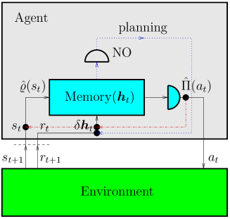
The agent is equipped with some quantum channel that acts as its memory whose properties can be modified by control parameters denoted by a vector $\bm{h}$. Examples of memory structures are listed in Fig. 2.

Figure 2: Examples for the agent’s memory as shown in Fig. 1. (a) unitary evolution of the percept states, (b) open system evolution due to interaction with a bath B, (c) composite memory with coupled subsystems for percept (S) and action (A) variables, (d) extends (c) to an open system evolution analogous to (b) extending (a). Further ancilla systems may be added (not shown), to account for, e.g., emotion degrees of freedom introduced in Briegel and las Cuevas (2012).

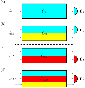
In Fig. 2 and in what follows, we refer to the memory operation by means of some unitary $\hat{U}$ for notational simplicity. Since any quantum process can be treated as unitary on an enlarged space, this is not a conceptual restriction. The agent interacts with an external environment in discrete cycles $t$. At the beginning of a cycle, the agent receives (via sensors) some percept $s$, which it encodes as a quantum state $\hat{\varrho}({s})$, in which its memory is prepared. After transformation of $\hat{\varrho}({s})$ by the memory channel, a quantum measurement is performed, where we assume for simplicity that the positive operator valued measure (POVM) $\{\hat{\Pi}\}$ describing this measurement is fixed. Depending on the outcome of this measurement, an action $a$ is selected and performed on the environment (via actuators), which completes the cycle. The environment reacts with a new percept and a reward $r$, which are perceived by the agent during the following cycle. Depending on the reward, some adjustments are made on the control parameters, which modify the properties of the memory channel (i.e., its “hardware”). This feedback loop is adapted from the classical schemes in Sutton and Barto (1998) and Russell and Norvig (2009), where the percepts $s$ in Fig. 1 correspond to the states in Sutton and Barto (1998). The agent’s interaction with the environment is here considered classical in the sense that percepts, actions and rewards are classical signals. The environment itself is not specified, it could represent, e.g., an experiment performed on a quantum system. Note that the environment in Fig. 1 is not to be confused with the bath in Fig. 2, which affects the memory channel but is not considered part of the agents “habitat”.

In addition to the external loop, we may also equip the agent with two types of internal feedback loops, which allow the agent to undertake what corresponds to “planning steps” in RL and “reflection” in PS. One type is similar to the external loop in that it involves state initialisations and measurements on the memory channel, but exploits that percepts, actions and rewards can be recorded and reproduced as a consequence of their classicality. The second type of internal loop does not involve state evolutions but requires some mathematical model of the memory channel itself, which is used to directly calculate a numerical objective (NO), whose value is used to alter the control parameters. Fig. 1 does not imply that all of these loops need to be simultaneously present, they are rather thought of either subprocesses within an overall agent scheme or possible modes of its operation. The numerical examples in this work will exclusively apply the external loop.

All three loops involve a parameter update $\delta\bm{h}$. In a “first-order” update, $\delta\bm{h}$ is proportional to some quantity that depends on the gradient $\bm{\nabla}\hat{U}$ of $\hat{U}$ with respect to $\bm{h}$. This gradient can either be computed directly from a memory model $\hat{U}(\bm{h})$ (i.e., from some symbolic expression of $\bm{\nabla}\hat{U}$ if available) or estimated from measurements. These “measurements” can be physical (POVM in Fig. 1) or numerical (NO in Fig. 1). For the estimation, one varies the components of $\bm{h}$ by a small amount and records the changes in the measured POVM or computed NO. Here are some elementary examples: (1a) A simulation of an external loop with a given model-based (i.e. analytic) $\bm{\nabla}\hat{U}$ is performed in Sec. V.1.1 (Fig. 5) for the case Fig. 2(c), in Sec. V.1.2 (Figs. 7-8) for the case Fig. 2(a), and in Sec. V.2 (Figs. 11 and 12) for the case Fig. 2(c). (1b) A simulation of an external loop with a POVM measurement-based $\bm{\nabla}\hat{U}$ is carried out in Clausen (2015) (Fig. 6) for the case Fig. 2(b). (2) A NO-based internal loop with a model-based $\bm{\nabla}\hat{U}$ is considered in Clausen et al. (2010) for the case Fig. 2(b) and in Clausen (2015) (Figs.2-4) for the case Fig. 2(a). (3) The POVM-based internal loop in Fig. 1 can be used to estimate $\bm{\nabla}\hat{U}$ in the absence of a model $\hat{U}(\bm{h})$ of the agent memory. To this end, one of the agent’s possibilities consists in inserting a number of internal cycles between each external cycle, where it repeatedly prepares its memory in the latest percept state and observes how a variation $\delta\bm{h}$ affects the measurement statistics. A discussion of this will be given in Sec. VI. Beyond these examples, all three loops can be interlaced with each other in various ways, analogous to the wealth of approaches reviewed in Sutton and Barto (1998).

III Update rule in parameter space

For the cycle-wise update of the control parameters $\bm{h}$ of the memory channel $\hat{U}$, we apply a rule

$$\bm{h}^{\prime}=\bm{h}+\kappa(\bm{h}_{\infty}-\bm{h})+{\alpha}{r}\sum_{k=0}^{t-1}(1-\eta)^{k}\bm{D}_{t-k},$$ (4)

inspired by the basic model of PS Briegel and las Cuevas (2012); Mautner et al. (2015). The number of components $h_{k}$ can range from one ($\bm{h}$ scalar) to infinity ($\bm{h}$ may represent a function or a vector of functions), and the $h_{k}$ can be assumed to be real-valued without loss of generality. In Briegel and las Cuevas (2012); Mautner et al. (2015), the components of $\bm{h}$ are the edge strengths of a directed graph representing a network of clips (the graph’s vertices). While these clips are considered sequences of remembered percepts and actions, the network itself abstracts from the clip’s internal contents. Our view of $\bm{h}$ as a control vector is one further simplification and generalization that may allow for but does not require the view of the memory as a network.

In (4), $\bm{h}$ and $\bm{h}^{\prime}$ are the control vectors before and after the update at cycle $t$, respectively. $\alpha$ $\!\geq$ $\!0$ is a (typically small) learning rate, and $r$ is the reward given at cycle $t$. $\kappa$ $\!\in$ $\![0,1]$ is a relaxation rate towards some equilibrium value $\bm{h}_{\infty}$ in the absence of rewards. This allows for what corresponds to the “forgetting” process suggested in Briegel and las Cuevas (2012); Mautner et al. (2015) to account for dissipation in an embodied implementation and deal with time-dependent environments. A natural possibility is to identify the value $\bm{h}_{0}$, with which the memory is initialised before the first cycle, with $\bm{h}_{\infty}$. This could be the zero vector $\bm{h}_{0}$ $\!=$ $\!\bm{0}$ yielding, e.g., the identity, $\hat{U}_{0}$ $\!=$ $\!\hat{U}(\bm{h}_{0})$ $\!=$ $\!\hat{I}$. The learning process will then be a reward-driven and generally stochastic navigation in parameter space $\{\bm{h}\}$ away from the zero vector $\bm{0}$. Lifted to $\hat{U}(\bm{h})$, this navigation starts at the identity $\hat{U}_{0}$ $\!=$ $\!\hat{I}$, that relaxes back to it in the prolonged absence of rewards. In this work, we consider static environments as in Melnikov et al. (2014), and hence always set $\kappa$ $\!=$ $\!0$. $\bm{D}_{t}$ is a difference vector. While some options for finite difference choices of $\bm{D}$ are outlined in Sec. VI, in all numerical examples within this work we restrict to the case, where $\bm{D}_{t}$ $\!=$ $\!\bm{\nabla}_{t}$ is a short-hand notation for the gradient

$$\bm{\nabla}_{t} = \bm{\nabla}p({a}|{s})_{t}=2\mathrm{Re}\bigl{\langle}\hat{U}^{\dagger}\hat{\Pi}({a})\bm{\nabla}\hat{U}\bigr{\rangle}_{t},$$ (5)

$$p({a}|{s}) = \mathrm{Tr}\bigl{[}\hat{U}\hat{\varrho}({s})\hat{U}^{\dagger}\hat{\Pi}({a})\bigr{]}=\bigl{\langle}\hat{U}^{\dagger}\hat{\Pi}({a})\hat{U}\bigr{\rangle},$$ (6)

with components $\frac{\partial{p}({a}|{s})}{\partial{h}_{k}}$ at cycle $t$. $p({a}|{s})$ is the probability of the obtained measurement outcome ${a}$ under the condition of the respective cycle’s percept state $\hat{\varrho}({s})$, where $\langle\cdots\rangle$ $\!\equiv$ $\!\mathrm{Tr}[\hat{\varrho}({s})\cdots]$ denotes the expectation value with respect to this state, and $\hat{\Pi}({a})$ is the member of the POVM that corresponds to measurement outcome $a$. The latter determines the action performed by the agent, and we use the same symbol for both. $(1$ $\!-$ $\!\eta)$ describes a backward-discount rate, which we have defined via a parameter $\eta$ $\!\in$ $\![0,1]$ to allow comparison with the glow mechanism introduced in Mautner et al. (2015). As mentioned above, the unitary transformation of the respective percept states $\hat{\varrho}({s}_{t})$ by the memory $\hat{U}$ $\!=$ $\!\hat{U}(\bm{h}_{t})$ at cycle $t$ in (6) refers in general to a larger (dilated) space. The dynamical semigroup of CPT maps proposed in Briegel and las Cuevas (2012) is included and can be recovered by referring to Fig. 2(d) [or alternatively Fig. 2(b)] and the assumption that

$$\hat{\varrho}({s}_{t})\quad(\equiv\hat{\varrho}_{\mathrm{SAB}}) = \hat{\varrho}_{\mathrm{SA}}({s}_{t})\otimes\hat{\varrho}_{\mathrm{B}},$$ (7)

$$\mathrm{Tr}_{\mathrm{B}}\left[\hat{U}\hat{\varrho}({s}_{t})\hat{U}^{\dagger}\right] = \mathrm{e}^{\mathcal{L}_{\mathrm{SA}}\Delta{T}^{(\mathrm{mem})}_{t}}\hat{\varrho}_{\mathrm{SA}}({s}_{t}),$$ (8)

where the physical memory evolution time $\Delta{T}^{(\mathrm{mem})}_{t}$ may depend on the cycle $t$ for a chosen parametrisation $\hat{U}(\bm{h})$ and must be distinguished from the agent response time that can additionally be affected by the potential involvement of internal loops in Fig. 1. The superoperator $\mathcal{L}$ $\!=$ $\!\mathcal{L}_{\mathrm{SA}}$, whose effect on $\hat{\varrho}$ $\!=$ $\!\hat{\varrho}_{\mathrm{SA}}$ is defined as a sum

$$\mathcal{L}\hat{\varrho}=-\mathrm{i}[\hat{H},\hat{\varrho}]+L\hat{\varrho},$$ (9)

generates in Briegel and las Cuevas (2012) a quantum walk and is given by a Hamiltonian $\hat{H}$ $\!=$ $\!\sum_{\{j,k\}\in{E}}\lambda_{jk}(\hat{c}_{kj}$ $\!+$ $\!\hat{c}_{kj}^{\dagger})$ $\!+$ $\!\sum_{j\in{V}}\epsilon_{j}\hat{c}_{jj}$ and a Lindbladian $L\hat{\varrho}$ $\!=$ $\!\sum_{\{j,k\}\in{E}}\kappa_{jk}(\hat{c}_{kj}\hat{\varrho}\hat{c}_{kj}^{\dagger}$ $\!-$ $\!\frac{1}{2}\{\hat{c}_{kj}^{\dagger}\hat{c}_{kj},\hat{\varrho}\})$, with $\hat{c}_{kj}$ $\!=$ $\!|{c}_{k}\rangle\langle{c}_{j}|$ performing transitions between clip states $|{c}_{l}\rangle$ $\!\in$ $\!\mathcal{H}_{\mathrm{SA}}$ along a graph $G$ $\!=$ $\!(V,E)$ consisting of a set $V$ of vertices and a set $E$ of edges. Since on the one hand, we here do not intend to necessarily represent $\hat{U}$ by a clip network, and on the other hand do not want to exclude from the outset situations involving time-dependent or non-Markovian bath effects Degenfeld-Schonburg and Hartmann (2014), we use the dilated $\hat{U}$ for simplicity instead. The set of all probabilities $p({a}|{s})$ in (6), i.e, the whole conditional distribution then defines the agent’s policy.

A reward given by the environment at time $t$ raises the question of the extent to which decisions made by the agent in the past have contributed to this respective reward. A heuristic method is to attribute all past decisions, but to a lesser degree the further the decision lies in the past. (Considering the agent’s life as a trajectory of subsequent percepts and actions, we could imagine the latest event trailing a decaying tail behind.) A detailed description of this idea is presented in Sutton and Barto (1998) in form of the eligibility traces, which can be implemented as accumulating or replacing traces. In the context of PS, a similar idea has been introduced as glow mechanism that can be implemented as edge or clip glow Mautner et al. (2015); Melnikov et al. (2014). In our context (4), we realise it by updating the control vector by a backward-discounted sum of gradients $\bm{\nabla}_{t-k}$ referring to percepts and actions involved in cycles that happened $k$ steps in the past. A sole update by the present gradient is included as limit $\eta$ $\!=$ $\!1$, for which (4) reduces to $\bm{h}^{\prime}$ $\!=$ $\!\bm{h}+\alpha{r}\bm{\nabla}p({a}|{s})$. This special case is sufficient for the invasion game, which we will consider in Sec. V, because at each cycle, the environment provides a feedback on the correctness of the agent’s decision by means of a non-zero reward. After that, we apply the general update (4) to a grid world task, where the agent’s goal cannot be achieved by a single action, and where the long term consequences of its individual decisions cannot be foreseen by the agent.

IV Relation to existing methods

In this section, we ignore the embodied implementation of our method as a quantum agent and briefly summarise and compare the update rules of the methods considered from a computational point of view. It should be stressed that RL is an umbrella term for problems that can be described as agent-environment interactions characterised by percepts/states, actions, and rewards. Hence all methods considered here are approaches to RL-problems. For notational convenience however, we here denote the standard value function-based methods as “RL” in a closer sense, keeping in mind that alternatives such as direct policy search deal with the same type of problem. The standard RL-methods successively approximate for each state or state action pair the expected return $R_{t}$ $\!=$ $\!\sum_{k=0}^{\infty}\gamma^{k}r_{t+k+1}$, i.e., a sum of future rewards $r$, forward-discounted by a discount rate $\gamma\in[0,1]$, that the agent is trying to maximise by policy learning. Corrections to the current estimates can be done by shifting them a bit towards actual rewards observed during an arbitrarily given number $n$ of future cycles, giving rise to “corrected $n$-step truncated returns” $R_{t}^{(n)}$ $\!=$ $\!{r}_{t+1}$ $\!+$ $\!\gamma{r}_{t+2}$ $\!+$ $\!\ldots$ $\!+$ $\!\gamma^{n-1}{r}_{t+n}$ $\!+$ $\!\gamma^{n}V_{t}(s_{t+n})$, where $V$ is the value function of the respective future state $s_{t+n}$ (analogous considerations hold for state action pairs). A weighted average of these gives the $\lambda$-return $R_{t}^{\lambda}$ $\!=$ $\!(1-\lambda)\sum_{n=1}^{\infty}\lambda^{n-1}R_{t}^{(n)}$, where $\lambda\in[0,1]$ is a parameter. In an equivalent “mechanistic” backward view, this gives rise to so-called eligibility traces. Since the glow mechanism of PS is closely related to this, we base our comparison on the $\lambda$-extension of one-step RL. $\lambda$ $\!=$ $\!0$ describes the limit of shallow sample backups of single-step learning, whereas the other limit $\lambda$ $\!=$ $\!1$ refers to the deep backups of Monte Carlo sampling, cf. Fig. 10.1 in Sutton and Barto (1998).

It would be a futile task to try a mapping of the numerous variations, extensions, or combinations with other approaches that have been discussed or are currently developed for the methods mentioned, such as actor-critic methods or planning in RL, or emotion, reflection, composition, generalization, or meta-learning in PS. In particular, our notion of basic PS implies a restriction to clips of length $L$ $\!=$ $\!1$, which reduces the edge strengths in the ECM clip network Fig. 2 in Briegel and las Cuevas (2012) to values $h(s,a)$ of state-action pairs. Furthermore, in this section, we restrict attention to the basic versions that are sufficient to treat the numerical example problems discussed in this work. We may think of tasks such as grid world, where actions lead to state transitions, until a terminal state has been reached, which ends the respective episode, cf. Sec. V.

IV.1 Tabular RL

In tabular RL, the updates are performed according to

$${e} \leftarrow ({e}+)1\quad[\mathrm{for}\;s\;\mathrm{or}\;(s,a)\;\mathrm{visited}],$$ (10)

$$U \leftarrow U+\alpha\left[r+\gamma{U}^{\prime}-{U}\right]{e}$$ (11)

$$=(1-\alpha{e})U+\alpha{e}r+\alpha\gamma{e}{U}^{\prime},$$

$${e} \leftarrow \gamma\lambda{e},$$ (12)

where ${U}$ $\!=$ $\!V(s)$ is a state value function in TD($\lambda$), cf. Fig. 7.7 in Sutton and Barto (1998), whereas ${U}$ $\!=$ $\!Q(s,a)$ is an action value function in SARSA($\lambda$), cf. Fig. 7.11 in Sutton and Barto (1998). ${U}^{\prime}$ $\!=$ $\!V(s^{\prime})$ [or ${U}^{\prime}$ $\!=$ $\!Q(s^{\prime},a^{\prime})$] refers to the value of the subsequent state or state action pair. ${e}$ $\!=$ $\!e(s)$ [${e}$ $\!=$ $\!e(s,a)$] denote the eligibility trace in TD($\lambda$) [SARSA($\lambda$)]. They can be updated by accumulating (${e}$ $\!\leftarrow$ $\!{e}$ $\!+$ $\!1$) or replacing (${e}$ $\!\leftarrow$ $\!1$) them in (10) (ignoring other options such as clearing traces Sutton and Barto (1998)). $\alpha$ is a learning rate, $r$ is the reward, and $\gamma$ the discount rate. Note that there are alternatives to (10)-(12). One of them is Q-learning, which can be derived from SARSA=SARSA($\lambda=0$) by updating $Q(s,a)$ off-policy, which simplifies a mathematical analysis. Since a Q($\lambda$)-extension of Q-learning is less straightforward, and there are convergence issues with respect to the gradient-ascent form discussed below (cf. Sec. 8.5 in Sutton and Barto (1998)), while the methods discussed here update on-policy, we restrict attention to (10)-(12).

IV.2 Gradient-ascent RL

Tabular RL is a special case of gradient-ascent RL, where $U$ is in the latter defined as in (10)-(12), except that it is given by a number of parameters $\theta_{k}$, which are combined to a vector $\bm{\theta}$. This parametrisation can be done arbitrarily. In the linear case, the parameters could be coefficients of, e.g., some (finite) function expansion, where the functions represent “features”. Hence ${U}$ $\!=$ $\!U(\bm{\theta})$, and the components of the gradient $\bm{\nabla}{U}$ are $\frac{\partial{U}}{\partial{\theta}_{k}}$, giving rise to a vector $\bm{e}$ of eligibility traces. The updates (10)-(12) now generalize to

$$\bm{e} \leftarrow \gamma\lambda\bm{e}+\bm{\nabla}{U},$$ (13)

$$\bm{\theta} \leftarrow \bm{\theta}+\alpha\left[r+\gamma{U}^{\prime}-{U}\right]\bm{e},$$ (14)

cf. Sec. 8 in Sutton and Barto (1998). While the eligibility traces are initialised with zero, the value functions (by means of their parameters) can be initialised arbitrarily in tabular and gradient-ascent RL.

IV.3 PS

Classical PS is a tabular model. By tabular we mean that the percepts and actions (and ultimately also clips of length $L$ $\!>$ $\!1$ in the ECM) form discrete (i.e., countable) sets, with the consequence, that the edge strengths $h$ can be combined to a table (matrix). Let us hence write the updates as summarised in App. A in a form allowing comparison with (10)-(12):

$${g} \leftarrow 1\quad[\mathrm{for}\;(s,a)\;\mathrm{visited}],$$ (15)

$${h} \leftarrow {h}+\lambda{g}+\gamma(h^{\mathrm{eq}}-h)$$ (16)

$$=(1-\gamma){h}+\lambda{g}+\gamma{h}^{\mathrm{eq}},$$

$${g} \leftarrow (1-\eta){g}.$$ (17)

In (15)-(17), we intentionally adopted the notation of PS. The glow parameter ${g}$ in (15)-(17) corresponds to a replacing trace ${e}$ in (10)-(12), with $(1$ $\!-$ $\!\eta)$ in (17) corresponding to $\gamma\lambda$ in (12), and $\lambda$ in (16) corresponds to the reward $r$ in (11). The discount rate $\gamma$ in (10)-(12) must not be confused with the dissipation or damping rate $\gamma\in[0,1]$ in (16). To avoid confusion, we denote the former by $\gamma_{\mathrm{disc}}$ and the latter by $\gamma_{\mathrm{damp}}$ for the remainder of this paragraph. If we disregard the absence of a learning rate in (15)-(17) [we may set $\alpha$ $\!=$ $\!1$ in (10)-(12)], we can obtain PS from tabular SARSA($\lambda$) by replacing the action value function $Q(s,a)$ with the connection weight $h(s,a)$, and the update of $h$ corresponding to the r.h.s. of (11),

$$(1-{g}){h}+\lambda{g}+\gamma_{\mathrm{disc}}{g}{h}^{\prime}={h}+\lambda{g}+(\gamma_{\mathrm{disc}}{h}^{\prime}-{h}){g},$$ (18)

with the update of $h$ given by the r.h.s. of (16),

$$(1\!-\!\gamma_{\mathrm{damp}}){h}\!+\!\lambda{g}\!+\!\gamma_{\mathrm{damp}}{h}^{\mathrm{eq}}\!=\!{h}\!+\!\lambda{g}\!+\!\gamma_{\mathrm{damp}}({h}^{\mathrm{eq}}\!-\!{h}).$$ (19)

In (10)-(12), RL is equipped with forward- and backward-discounting mechanisms, as becomes apparent in the product $\gamma_{\mathrm{disc}}\lambda$ in (12). Disabling the accumulation of forward-discounted future rewards (that give rise in RL to the return mentioned above) by setting $\gamma_{\mathrm{disc}}$ $\!=$ $\!0$ reduces (18) to $(1$ $\!-$ $\!g){h}$ $\!+$ $\!\lambda{g}$, while setting ${h}^{\mathrm{eq}}$ $\!=$ $\!0$ reduces (19) to $(1$ $\!-$ $\!\gamma_{\mathrm{damp}}){h}$ $\!+$ $\!\lambda{g}$. These expressions are very similar, except that in PS, the constant $\gamma_{\mathrm{damp}}$ has taken the place of $g$ in RL, so that $(1$ $\!-$ $\!\gamma_{\mathrm{damp}})$ determines the range of backward-discounting in (39). Since in (39), it is the respective past excitations (glowing rewards) $r_{t}$ $\!=$ $\!g_{t}\lambda_{t}$, rather than the rewards $\lambda_{t}$ themselves, which is summed up, damping and glow play a similar role. On the other hand, the factor $(1$ $\!-$ $\!\eta)$ takes in PS the place of $\gamma_{\mathrm{disc}}\lambda$ in (12), which becomes zero together with $\gamma_{\mathrm{disc}}$, as mentioned.

IV.4 Method presented here

The update rule (4) is implemented as

$$\bm{e} \leftarrow (1-\eta)\bm{e}+\bm{\nabla}\,p(a|s),$$ (20)

$$\bm{h} \leftarrow \bm{h}+{\alpha}{r}\bm{e}+\kappa(\bm{h}_{\infty}-\bm{h}),$$ (21)

which can be obtained from gradient-ascent SARSA($\lambda$) by replacing in (13)-(14) the action value function $Q(s,a)$ with the conditional probability $p(a|s)$, renaming $\bm{\theta}$ as $\bm{h}$, replacing $\gamma\lambda$ in (13) with $(1$ $\!-$ $\!\eta)$, and replacing in (14) the term $\alpha\bigl{[}\gamma{p}(a^{\prime}|s^{\prime})$ $\!-$ $\!{p}(a|s)\bigr{]}\bm{e}$ with $\kappa(\bm{h}_{\infty}-$ $\!\bm{h})$. The latter replacement is similar to the change from (18) to (19), where $\kappa$ in (21) corresponds to $\gamma$ in (16). Analogous to the comments following (18) and (19), in the case $\gamma$ $\!=$ $\!0$, the update corresponding to the r.h.s. of (14) becomes $(\bm{h}$ $\!-$ $\!\alpha{p}\bm{e})$ $\!+$ $\!\alpha{r}\bm{e}$, whereas for $\bm{h}_{\infty}$ $\!=$ $\!0$, the r.h.s. of (21) reduces to $(1$ $\!-$ $\!\kappa)\bm{h}$ $\!+$ $\!\alpha{r}\bm{e}$. Similar to the tabular case, the constant damping rate $\kappa$ has in our method taken the place of $\alpha{p}\bm{e}$ in gradient-ascent RL.

IV.5 Can PS be recovered from our approach?

Our method (20)-(21) replaces a value function with a conditional probability (6), whereas the edge strengths in PS remain value function-like quantities. While tabular RL can be recovered from gradient-ascent RL, one hence cannot expect to recover the basic PS update rule (15)-(17) as a special case of our scheme, despite replacements analogous to (18)-(19). To understand the difference, we restrict attention to an invasion game - like case as shown in Fig. 3 as the simplest example, cf. also Sec. V for details.

Figure 3: Transition strengths ${h}_{kl}$ for an invasion game-like task with states (which are here synonymous to percept-clips) $s_{k}$ and action clips $a_{l}$. The strengthening of a rewarded transition (here ${h}_{22}$) is in an update (26) based on the gradient of $p(a_{j=2}|s_{i=2})$ accompanied by a weakening of the respective transitions to the remaining actions (here ${h}_{21}$ and ${h}_{23}$), which is absent in PS, cf. (27).

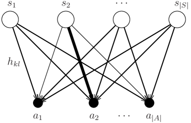
Since here, each episode lasts one cycle, we disable both the eligibility trace/glow mechanism by setting $\eta$ $\!=$ $\!1$ in (20)-(21) and (15)-(17). As shown in Fig. 3, we are given a set of states $\{s_{1},s_{2},\ldots,s_{|S|}\}$, each of which allows one out of a set of actions $\{a_{1},a_{2},\ldots,a_{|A|}\}$. Consider a cycle, where from state $s_{i}$, an action $a_{j}$ is selected. If the transition probabilities

$$p_{ij}=p(a_{j}|s_{i})=\frac{\Pi({h}_{ij})}{c_{i}},\quad{c}_{i}=\sum_{j}\Pi({h}_{ij}),$$ (22)

are given by some policy function $\Pi$, then the components of the r.h.s. of (20) read

$$e_{kl|ij}=\frac{\partial{p}_{ij}}{\partial{h}_{kl}}=\frac{\delta_{ik}\Pi^{\prime}({h}_{kl})}{c_{i}^{2}}\bigl{[}\delta_{jl}c_{i}-\Pi({h}_{ij})\bigr{]},$$ (23)

with which the components of the update (21) become

$${h}_{kl}\leftarrow(1-\kappa){h}_{kl}+\alpha{r}e_{kl|ij}+\kappa{h}_{kl}^{\mathrm{eq}},$$ (24)

where we have renamed $\bm{h}_{\infty}$ as $\bm{h}^{\mathrm{eq}}$. An observer ignorant of the transitions $i$ $\!\to$ $\!j$ and the corresponding probabilities $p_{ij}$ notices no change,

$$\sum_{ij}e_{kl|ij}=0.$$ (25)

In the special case $\Pi({h}_{kl})$ $\!=$ $\!{h}_{kl}$, we can simplify (23) to

$$e_{kl|ij}=\frac{1}{c_{i}}\left(\delta_{ik}\delta_{jl}-\frac{{h}_{ij}}{c_{i}}\delta_{ik}\right).$$ (26)

From (26) we see that in the gradient method, the strengthening of the ${h}_{ij}$-edge is accompanied with a weakening of those edges ${h}_{kl}$ connecting the respective state $k$ $\!=$ $\!i$ with different actions $l$ $\!\neq$ $\!j$. As a consequence, the ${h}_{kl}$ may become negative, even if $\Pi({h}_{kl})$ $\!=$ $\!{h}_{kl}$ and the rewards are non-negative. This weakening is absent in basic PS (16), where the corresponding update is independent of the policy function $\Pi$ and given by

$${h}_{kl} \leftarrow {h}_{kl}-\gamma({h}_{kl}-{h}_{kl}^{\mathrm{eq}})+\lambda\delta_{ik}\delta_{jl}$$ (27)

$$= (1-\gamma){h}_{kl}+\lambda\delta_{ik}\delta_{jl}+\gamma{h}_{kl}^{\mathrm{eq}}.$$

Hence, ${h}_{kl}$ $\!\geq$ $\!0$ as long as the rewards are non-negative. In any case, choice of a non-negative policy function $\Pi({h}_{kl})$ renders the methods independent of a need of positive edge strengths. [Note that a similar problem occurs if the parameters in a memory consisting of alternating layers such as $\hat{U}$ $\!=$ $\!\cdots\mathrm{e}^{-\mathrm{i}{t}_{3}\hat{H}^{(1)}}\mathrm{e}^{-\mathrm{i}{t}_{2}\hat{H}^{(2)}}\mathrm{e}^{-\mathrm{i}{t}_{1}\hat{H}^{(1)}}$, cf. App. B.2, refer to non-negative physical quantities $t_{k}$. In Clausen (2015), this has been solved by using an exponential function such as ${t}_{k}$ $\!=$ $\!\mathrm{e}^{{h}_{k}}$ for parametrisation in terms of the controls $h_{k}$. In this work, we identify the $h_{k}$ directly with the $t_{k}$ for simplicity, which, if the $h_{k}$ are to be interpreted as non-negative quantities, doubles the set of physically applied Hamiltonians from $\{\hat{H}^{(1,2)}\}$ to $\{\pm\hat{H}^{(1,2)}\}$.]

IV.6 Discussion

The relations between the different methods are summarised in Fig. 4.

Figure 4: Tabular RL (10)-(12) is a special case of gradient-ascent RL (13)-(14). Replacing updates based on values of subsequent states with updates based on a physical damping term yields basic PS (15)-(17) and the method presented here (20)-(21), which however uses a conditional probability (6) instead of a value function, hence the basic PS update rule cannot be recovered from our approach, as explained in Sec. IV.5.

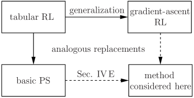
If one considers the ECM as the core element of PS rather than a specific update rule, one could alternatively adopt, e.g., the tabular SARSA($\lambda$)-update rule. The picture of a random walk in clip space does not contradict the general framework of RL-problems. One may understand the clips as the agent’s states (which must be distinguished from the percepts). The same holds for the gradient-ascent generalization, which, in physical terms, could be considered as “continuous variable RL”. On the one hand, we could equally well apply, e.g., the gradient-ascent SARSA($\lambda$)-update instead of our rule. On the other hand, before trying to create algorithmic extensions such as those mentioned at the beginning of this section for tabular RL and PS, one should first investigate whether and how such extensions are accomplished in any existing gradient-ascent RL variants.

V Examples

V.1 Invasion game

In what follows, we consider a simple invasion game as treated in Briegel and las Cuevas (2012). An attacker randomly chooses one out of two possible symbols $\{\Leftarrow,\Rightarrow\}$ which signals the direction in which it intends to move. The chosen symbol may represent, e.g., a head turn and is visible to the defender, whose task is to learn to move in the same direction, which is required to block the attacker. We approach this learning task as an external loop in Fig. 1 with a closed system (i.e., bath-less) memory [cases (a) and (c) in Fig. 2], described within a 4-dimensional Hilbert space. The control parameters are updated according to (4) in the absence of relaxation ($\kappa$ $\!=$ $\!0$) and gradient glow ($\eta$ $\!=$ $\!1$). The update is done with an analytic $\bm{\nabla}\hat{U}$ as described in App. B.2, where the memory consists of alternating layers, $\hat{U}$ $\!=$ $\!\cdots\mathrm{e}^{-\mathrm{i}{h}_{3}\hat{H}^{(1)}}\mathrm{e}^{-\mathrm{i}{h}_{2}\hat{H}^{(2)}}\mathrm{e}^{-\mathrm{i}{h}_{1}\hat{H}^{(1)}}$, with a given number of controls $h_{1},\ldots,h_{n}$. At the beginning of the first cycle, the memory is initialised as identity. For the two Hamiltonians $\hat{H}^{(1)}$ and $\hat{H}^{(2)}$, we distinguish (I) a general case, where $\hat{H}^{(1)}$ and $\hat{H}^{(2)}$ are two given (randomly generated) 4-rowed Hamiltonians acting on the total Hilbert space and (II) a more specialised case, in which they have the form

$$\hat{H}^{(1)} = \hat{H}^{(1)}_{\mathrm{S}}\otimes\hat{I}_{\mathrm{A}}+\hat{I}_{\mathrm{S}}\otimes\hat{H}^{(1)}_{\mathrm{A}},$$ (28)

$$\hat{H}^{(2)} = \hat{H}^{(2)}_{\mathrm{S}}\otimes\hat{H}^{(2)}_{\mathrm{A}},$$ (29)

where $\hat{H}^{(1)}_{\mathrm{S}}$, $\hat{H}^{(1)}_{\mathrm{A}}$, $\hat{H}^{(2)}_{\mathrm{S}}$, $\hat{H}^{(2)}_{\mathrm{A}}$ are four given (randomly generated) 2-rowed Hamiltonians acting on the percept (S) and action (A) subsystems, respectively, with $\hat{I}$ denoting the identity. The latter case (II) refers to a physical implementation of Fig. 2(c) as a bath-mediated interaction of the S and A subsystems that is obtained from the setup Fig. 2(d) by eliminating the bath Clausen (2015). It has been included here to demonstrate that this special structure as considered in Clausen (2015) may be applied in the present context, but this is not mandatory. While the Hamiltonians have been chosen in both cases (I) and (II) at random to avoid shifting focus towards a specific physical realization, in an experimental setup, the respective laboratory Hamiltonians will take their place (assuming that they generate universal gates in the sense of Lloyd (1995), which is almost surely the case for a random choice).

V.1.1 2 percepts $\to$ 2 actions

We start with a basic version of the game with 2 possible percepts (the two symbols shown by the attacker) and 2 possible actions (the two moves of the defender). For each percept, there is hence exactly one correct action, which is to be identified. The memory applied is shown in Fig. 2(c), and the different input states are

$$\hat{\varrho} = \hat{\varrho}_{\mathrm{S}}\otimes\hat{\varrho}_{\mathrm{A}},\quad\hat{\varrho}_{\mathrm{S}}=|{s}\rangle\langle{s}|,$$ (30)

$$\hat{\varrho}_{\mathrm{A}} = p_{\mathrm{coh}}|\varphi\rangle\langle\varphi|+(1-p_{\mathrm{coh}})\frac{1}{d_{\mathrm{A}}}\hat{I}_{\mathrm{A}},\quad$$ (31)

$$|\varphi\rangle = \frac{1}{\sqrt{d_{\mathrm{A}}}}\sum_{a}|{a}\rangle,$$ (32)

where $d_{\mathrm{A}}$ $\!=$ $\!\mathrm{dim}\mathcal{H}_{\mathrm{A}}$ $\!=$ $\!2$ is given by the number of actions. $|s\rangle$ and $|a\rangle$ can both be one of the two orthonormal states $|0\rangle$ or $|1\rangle$ of the S and A subsystem, respectively. The POVM consists of the elements

$$\hat{\Pi}(a)=\hat{I}_{\mathrm{S}}\otimes|{a}\rangle_{\mathrm{A}}\langle{a}|.$$ (33)

Choosing the correct (wrong) action [i.e. $a$ $\!=$ $\!s$ ($a$ $\!\neq$ $\!s$) in (33) and (30)] returns a reward of $r$ $\!=$ $\!+1$ ($r$ $\!=$ $\!-1$).

Fig. 5 shows the average reward $\overline{r}$ received at each cycle, where the averaging is performed over an ensemble of $10^{3}$ independent agents.

Figure 5: Average reward $\overline{r}$ as a function of the number of cycles for an invasion game (2 symbols, 2 moves), learning rate $\alpha$ $\!=$ $\!10^{-3}$, with a reward of +1 (-1) for a correct (false) move, averaged over $10^{3}$ agents. The input states and POVM are given by Eqs. (30) and (33), respectively. (a) The 6 graphs from bottom to top correspond to 1, 2, 3, 4, 8, and 16 controls, respectively, with $p_{\mathrm{coh}}$ $\!=$ $\!1$ in (31). (b) 16 controls, where after $4\cdot 10^{3}$ cycles the meaning of the symbols is reversed. The 5 graphs from bottom to top correspond in Eq. (31) to $p_{\mathrm{coh}}$= 0, 0.25, 0.5, 0.75, and 1, respectively. (c) applies 32 controls and $p_{\mathrm{coh}}$ $\!=$ $\!1$, but refers to case (II) described by (28) and (29), whereas Figs. 5(a,b) refer to case (I).

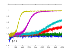
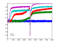
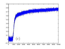
$(\overline{r}+1)/2$ is hence an estimate of the defender’s probability to block an attack. Referring to pure states in (31), Fig. 5(a) shows the increase of learning speed with the number of controls. Significant learning progress begins only after some initial period of stagnation. From the viewpoint of control theory, the identity, in which the memory is initialised, may lie on a “near-flat ground” (valley), which must first be left before progress can be made Goerz et al. (2015). Asymptotically, perfect blocking can be achieved once the memory becomes controllable, i.e., if the number of controls equals (or exceeds) the number of group generators. Fig. 5(b) demonstrates the need of a pure input state $\hat{\varrho}_{\mathrm{A}}$ in (31) of the action subsystem A rather than an incoherent mixture. After the agent in Fig. 5(b) had some time to adapt to the attacker, the meaning of the symbols is suddenly interchanged, and the agent must now learn to move in the opposite direction. This relearning differs from the preceding learning period in the absence of the mentioned initial stagnation phase, which supports the above hypothesis of the proposed valley, the agent has left during the initial learning. This plot is motivated by Fig. 5 in Briegel and las Cuevas (2012) describing classical PS. Although the different behaviour in the classical case suggests that this is an effect specific to quantum control, the phenomenon, that a dynamically changing environment can facilitate learning in later stages appears to be more general Clausen (2016). While Figs. 5(a,b) refer to case (I) described before (28), Fig. 5(c) refers to the restricted case (II), which appears to impede learning. In the simulations of the following Sec. V.1.2, which all refer to case (II), this is resolved by applying a 10 times larger negative reward for each wrong action. This demonstrates the flexibility in approaching RL problems offered by the freedom to allocate rewards in a suitable way.

V.1.2 4 percepts $\to$ 4 or 2 actions

We now consider a version with 4 percepts, referring to an attacker presenting each of its two symbols in two colors at random. Since we want to keep the Hilbert space dimension unchanged (rather than doubling it by adding the color category) for better comparison of the effect of the number of controls on the learning curve, we must apply a memory as shown in Fig. 2(a). The 4 percepts are encoded as tensor products of orthonormal projectors

$$\hat{\varrho}_{jk}=|{j}\rangle\langle{j}|\otimes|{k}\rangle\langle{k}|,$$ (34)

where $j$ $\!=$ $\!0,1$ ($k$ $\!=$ $\!0,1$) refers to the symbol (color). The POVM operators are the 4 projectors

$$\hat{\Pi}_{jk}=\hat{U}_{\mathrm{T}}\hat{\varrho}_{jk}\hat{U}_{\mathrm{T}}^{\dagger},$$ (35)

where $\hat{U}_{\mathrm{T}}$ is a given (randomly generated) 4-rowed target unitary acting on the total system. The memory in Fig. 2(a) is hence still composed of two subsystems referring to the two percept categories ‘symbol’ and ‘color’, but both subsystem’s initial state depends on the respective percept, and both are measured afterwards. The differences between the setup discussed in the previous Sec. V.1.1 and the two setups discussed in the present Sec. V.1.2 are summarised in Fig. 6.

Figure 6: Setups for the invasion game as investigated numerically in Sec. V.1. Setup (a) involves 2 percepts (symbols) and 2 actions (moves) as discussed in Sec. V.1.1 (Fig. 5). Setup (b) involves 4 percepts consisting of 2 two-colored symbols and 2 measurements yielding 4 different outcomes described by $(j,k=0,1)$ as discussed in Sec. V.1.2 and determining either 4 [Fig. 7(a) and Fig. 8] or – if outcome $k$ is ignored – 2 [Fig. 7(b)] possible actions (moves). While setup (a) refers to Fig. 2(c), setup (b) must refer to Fig. 2(a), if we want to keep the same Hilbert space dimension of 4 for both setups, which allows better comparison of the effect of the number of controls on the learning curve. Setup (c) involves a continuum of percepts consisting of 2 arbitrary-colored symbols and 2 actions (moves) as discussed in Sec. V.1.3 (Fig. 9). In setup (c), separate subsystems are used for all 3 categories, hence it refers to Fig. 2(c), and the Hilbert space dimension becomes 8.

Fig. 7 shows the average reward $\overline{r}$ received at each cycle, where the averaging is performed over an ensemble of $10^{3}$ independent agents, analogous to Fig. 5.

Figure 7: Average reward $\overline{r}$ as a function of the number of cycles for an invasion game (2 symbols in 2 colors), learning rate $\alpha$ $\!=$ $\!10^{-2}$, with a reward of +1 (-10) for a correct (false) move, averaged over $10^{3}$ agents. The input states and POVM are given by Eqs. (34) and (35), respectively. The graphs correspond to 1, 2, 3, 4, 8, 16, and 32 controls, as marked on the right. (a) Out of 4 possible moves, the defender must learn the correct one for each symbol and color. After $5\cdot 10^{3}$ cycles, the meanings of the symbols as well as the colors are reversed. (b) Out of 2 possible moves, the defender must learn the correct one for each symbol, whereas the color is irrelevant. For the first $5\cdot 10^{3}$ cycles, only symbols in a single color are presented, whereas for the remaining cycles, they are shown randomly in both colors.

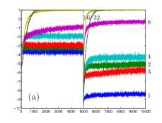
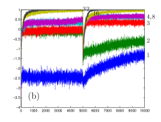
Note that in this Sec. V.1.2, all figures refer to case (II) described by (28) and (29), where S and A now denote symbol and color, respectively. To account for this [cf. the comments on Fig. 5(c) above], a reward of $r$ $\!=$ $\!-10$ (instead of -1) is now given for a wrong action. The estimate of the defender’s probability to block an attack is hence now $(\overline{r}+10)/11$.

In Fig. 7(a), the defender can choose between 4 moves, where for each percept, there is exactly one correct action [i.e., detecting $\hat{\Pi}_{jk}$ ($\hat{\Pi}_{j^{\prime}{k}^{\prime}}$ $\!\neq$ $\!\hat{\Pi}_{jk}$) for $\hat{\varrho}_{jk}$ in (35) and (34) returns a reward of $r$ $\!=$ $\!+1$ ($r$ $\!=$ $\!-10$)]. After $5\cdot 10^{3}$ cycles, symbol $j$ and color $k$ are read as symbol $1-j$ and color $1-k$, respectively, similar to the manipulations in Fig. 5 in Briegel and las Cuevas (2012). In Fig. 7(b), the defender can choose between 2 moves, where for each symbol (relevant category), there is exactly one correct action, irrespective of its color (irrelevant category) [i.e., detecting $\hat{\Pi}_{j}$ $\!=$ $\!\sum_{k=0}^{1}\hat{\Pi}_{jk}$ ($\hat{\Pi}_{j^{\prime}}$ $\!\neq$ $\!\hat{\Pi}_{j}$) for $\hat{\varrho}_{jk}$ in (35) and (34) returns a reward of $r$ $\!=$ $\!+1$ ($r$ $\!=$ $\!-10$)]. The second color is added only after $5\cdot 10^{3}$ cycles, analogous to Fig. 6 in Briegel and las Cuevas (2012). [Note that the mentioned initial stagnation phase in Fig. 5 is not visible in Fig. 7, which is attributed to the choice of parameters (rewards), accelerating the initial learning.]

Figs. 5(b) and 7 are all motivated by Figs. 5 and 6 in Briegel and las Cuevas (2012) and confirm that the agent’s adaptation to changing environments is recovered in our quantum control context. In addition, Figs. 5(a) and 7 show the behaviour of an underactuated memory, where the number of controls is insufficient for its full controllability. Since a $U(n)$-matrix is determined by $n^{2}$ real parameters, and a global phase can be disregarded (so that we can restrict to SU($n$)-matrices), $n^{2}$ $\!-$ $\!1$ controls are sufficient, i.e., 15 for our invasion game, as mentioned above.

In (35), the measurements are made in a basis rotated by a randomly given unitary $\hat{U}_{\mathrm{T}}$, which serves two purposes. On the one hand, it is required to ensure that the agent starts at the beginning of the first cycle with a policy that does not give exclusive preference to certain actions that follow from symmetries of the (identity-) initialised memory. This is a flaw of Fig. 2(a) and can be overcome by using Fig. 2(c) instead (cf. a more detailed discussion in the grid world example below). On the other hand, $\hat{U}_{\mathrm{T}}$ serves as a given target in our discussion Sec. I.2, where we consider the agent learning as a navigation of its memory $\hat{U}$, cf. also Fig. 6(b). Fig. 8 compares the case, where the agent is always fed with percept states drawn from one single ONB defined via (34) with the case, where the percept states are drawn randomly, i.e., taking $\hat{U}_{\mathrm{R}}\hat{\varrho}_{jk}\hat{U}_{\mathrm{R}}^{\dagger}$ with a random unitary $\hat{U}_{\mathrm{R}}$ as explained in Sec. I.2 instead of (34). Note that in Fig. 8, we generate a new random $\hat{U}_{\mathrm{R}}$ at each cycle, although a fixed set of dim$\mathcal{H}$ (4 in our case) such $\hat{U}_{\mathrm{R}}$ is sufficient as mentioned in Sec. I.2.

Figure 8: (a) Reward $r$, (b) fidelity $F$ defined in (48), and (c) squared distance $D$ defined in (47), where the overline denotes the ensemble average over $10^{3}$ agents for the setup as in Fig. 7(a) (i.e., 4 percepts and 4 actions) with 16 controls but without the reversal of meaning. The initial memory states are drawn from either a single or multiple orthonormal bases.

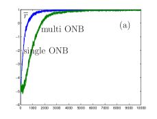
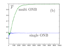
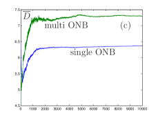
Fidelity $F$ and squared distance $D$ are defined in (48) and (47), where $\hat{U}$ represents the agent memory and $\hat{U}_{\mathrm{T}}$ the target unitary. Each cycle’s update constitutes a single navigation step in the unitary group [U(4) in our example]. If, for a single ONB, after a number of cycles, the average reward has approached unity, $\hat{U}$ has reached a close neighbourhood of any unitary of the form $\hat{U}_{2}^{\prime}\hat{U}_{\mathrm{T}}\hat{U}_{1}$, where $\hat{U}_{2}^{\prime}$ $\!=$ $\!\hat{U}_{\mathrm{T}}\hat{U}_{2}\hat{U}_{\mathrm{T}}^{\dagger}$ with $\hat{U}_{1}$ and $\hat{U}_{2}$ being undetermined 4-rowed unitary matrices diagonal in the common eigenbasis of the $\hat{\varrho}_{jk}$ (i.e., the “computational basis”). Fig. 8(a) shows that for a solution of the invasion game, a fixed ONB is sufficient. Drawing the percept states randomly, so that the set of all percept states is linearly dependent, does not affect the agent’s ability to achieve perfect blocking efficiency, but slows down the learning process. The single ONB case allows for a larger set of $\hat{U}$ $\!=$ $\!\hat{U}_{2}^{\prime}\hat{U}_{\mathrm{T}}\hat{U}_{1}$ with respect to $\hat{U}_{\mathrm{T}}$, as becomes evident in Fig. 8(b), so that navigation of $\hat{U}$ from the identity to a member of this set takes less time (as measured in cycles). The only freedom left in the case of multiple ONBs is a global phase of $\hat{U}$, which remains undefined: navigation of $\hat{U}$ towards $\hat{U}_{\mathrm{T}}$ with respect to the squared Euclidean distance $D$ is not required for the learning tasks discussed, as evidenced by Fig. 8(c).

V.1.3 Neverending-color scenario

In Sec. V.1.2 we considered the case, where the symbols are presented in two different colors, as depicted in Fig. 6(b). The original motivation for introducing colors as an additional percept category was to demonstrate the agent’s ability to learn that they are irrelevant Briegel and las Cuevas (2012). In contrast, Melnikov et al. (2015) present a “neverending-color scenario”, where at each cycle, the respective symbol is presented in a new color. It is shown that while the basic PS-agent is in this case unable to learn at all, it becomes able to generalize (abstract) from the colors, if it is enhanced by a wildcard mechanism. The latter consists in adding an additional (wildcard “$\#$”) value to each percept category, and inserting between the input layer of percept clips and the output layer of action clips hidden layers of wildcard percept clips, in which some of the percept categories attain the wildcard value. The creation of these wildcard clips follows predefined deterministic rules, and the transitions from percept to action clips take then place via the hidden layers. (The notion of layers in the general ECM clip network Fig. 2 in Briegel and las Cuevas (2012) follows from restricting to clips of length $L$ $\!=$ $\!1$).

Since the use of wildcard clips is an integrated mechanism within PS (inspired by learning classifier systems), the question is raised how similar ideas could be implemented in our context. For a memory Fig. 2(c), we could, e.g., attribute one of the levels (such as the respective ground state) of the quantum system of each percept category $\mathrm{S}_{i}$ to the wildcard-level $|\#\rangle_{i}$, so that the percept space $\mathcal{H}_{\mathrm{S}}$ $\!=$ $\!\otimes\mathcal{H}_{\mathrm{S}_{i}}$ is enlarged to $\mathcal{H}_{\mathrm{S}}$ $\!=$ $\!\otimes(\mathcal{H}_{\mathrm{S}_{i}}$ $\!\oplus$ $\!\mathcal{H}_{\#_{i}})$, where the $\mathcal{H}_{\#_{i}}$ are one-dimensional.

Instead of this, let us simply make use of the built-in generalization capacity of a quantum agent resulting from its coding of percepts as quantum states, which is much in the sense of Sec. 8 in Sutton and Barto (1998), where the percepts can be arbitrarily real-valued rather than being drawn from a countable or finite value set. Consider the setup shown in Fig. 6(c), whose percept system includes a symbol and a color category and refers to a memory structure Fig. 2(c). To allow for infinite colors, we could apply a color quantum system with infinite levels $\mathcal{H}_{\infty}$ (such as an oscillator-type system), which is initialized at each cycle in a new state drawn from a fixed ONB (such as a higher number state for an oscillator-type system). While such a scheme becomes more challenging to control, because the control vector $\bm{h}$ has an infinite number of components [we may replace it with a continuous control function $h(t)$], it still ignores the fact that colors (as most percept categories in general) are not countable. With this in mind, we can take the notion of colors literally and, to put it simply, code them in some appropriate color space such as RGB, where three parameters correspond to the red-, green-, and blue-signals of the agent’s eye sensors. This suggests to encode a color as a mixed state of a two-level system, which is also given by three real-valued parameters (determining its location in the Bloch ball). The generalization from two colors to all RGB-colors then corresponds to the generalization from a classical to a quantum bit. In our setup, it is hence sufficient to apply a two-level system for the color category and initialize it at each cycle in a randomly chosen mixed state $\hat{\varrho}_{\mathrm{C}}$ (for neverending colors) rather than a (pure) state randomly drawn from a single ONB (for two colors), whereas no changes are required on the agent’s memory configuration itself. Fig. 9 demonstrates the learning process.

Figure 9: (a) Reward $r$ and (b) length $|\bm{h}|$ of the control vector as a function of the number of cycles for a single agent Fig. 6(c) playing an invasion game with 2 symbols, presented in a continuum of neverending colors, and 2 moves. A reward of +1 (-10) is given for each correct (false) move. The agent applies 64 controls with a learning rate of $\alpha$ $\!=$ $\!10^{-2}$ in an alternating layer scheme App. B.2 defined by two (Schmidt-orthonormalized) 8-rowed random Hamiltonians.

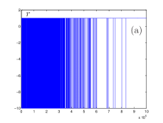
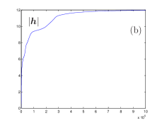
Similar to Fig. 8, random initialization slows down the learning process, so that we restrict to a single agent in Fig. 9, rather than an ensemble average. As illustrated in Fig. 9(a), the agent’s response becomes near-deterministic after about $10^{6}$ cycles, irrespective of the color. Fig. 9(b) illustrates in the example of the Euclidean length of the control vector $|\bm{h}|$ $\!=$ $\!\sqrt{\bm{h}^{\mathrm{T}}\cdot\bm{h}}$, that the navigation, which starts at $\bm{h}_{0}$ $\!=$ $\!\bm{0}$, eventually comes to rest. While the random $\hat{\varrho}_{\mathrm{C}}$ are drawn such that a positive probability is attributed to every volume element in the Bloch ball, we did not care about drawing them with a uniform probability density, since mapping of an RGB-space of color (as a perceptual property) to the Bloch ball is not uniquely defined.

The ability to learn to distinguish between relevant $\mathrm{S}_{\mathrm{rel}}$ and an arbitrary number of irrelevant percept categories $\mathrm{S}_{\mathrm{irr}}$ as discussed in Melnikov et al. (2015) is of particular relevance for a quantum agent, where the irrelevant percept categories can be understood as adopting the role of a bath as shown in Figs. 2(b) and (d). Here, a formal solution consists in a decoupled $\hat{U}_{\mathrm{SA}}$ $\!=$ $\!\hat{U}_{\mathrm{S_{rel}A}}$ $\!\otimes$ $\!\hat{U}_{\mathrm{S_{irr}}}$.

V.2 Grid world

In what follows, we consider an arrangement of 8 grid cells as shown in Fig. 10.

Figure 10: $(3\times 3)$-grid world with an obstacle (black cell). The arrows show the optimal policy for the shortest path to G, and the numbers present the policy numerically obtained with the agent Fig. 11(d) after $10^{4}$ episodes. The red numbers in parentheses are the relevant different values obtained after $10^{5}$ episodes, if the agent starts each episode from a random cell, rather than always at S.

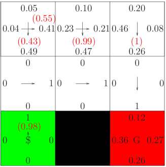
The agent’s task is to find the shortest route to a goal cell G, where at each step, only moves to an adjacent cell in four directions (left, right, up, down) are allowed. If the agent hits a boundary of the grid or the black cell, which is considered an obstacle, its location remains unchanged.

This external classical navigation task constitutes a learning problem, because situations/percepts (present location) must be mapped to decisions/actions (direction to go). The agent only perceives whether or not it has arrived at the goal cell. It has no access to a “bird’s perspective” which would allow immediate exact location of the goal. It also has no access to a measure of goal distance or fidelity (as in the case of the internal NO-based loop regarding its own quantum memory in Fig. 1), which prevents the use of external gradient information that could be obtained by testing the nearest neighbourhood of the present location. One can thus distinguish two objectives: (a) locating the goal and (b) finding a shortest route to it. This task constitutes a RL type problem, whose composite “two-objective” structure is approached by nesting iterations. The individual action selections, i.e., choices of moves, correspond to the cycles in Fig. 1. Sequences of cycles form episodes, which are terminated only once objective (a) has been solved. Objective (b) is solved by sequences of episodes, which allow the agent to gradually solve objective (a) more efficiently and find an optimal policy. In Fig. 10, the policy consists of a set of four probabilities for each cell, with which a corresponding move should be made from there. The optimal policy corresponding to the shortest route to G is indicated by the arrows in Fig. 10.

This grid world extends the above decision game in two aspects: (a) The optimal policy is in contrast to the decision game not deterministic, as indicated by the double arrows in the upper left and middle cell in Fig. 10. (b) Depending on where the agent starts, more than a single move is required to reach G in general, preventing the agent from obtaining an immediate environmental feedback on the correctness of each individual move it makes. This second aspect leads to the mentioned notion of episodes. In what follows, we always place the agent at a fixed start cell S at the beginning of each episode, which is sufficient for learning the shortest path from S to G. While in the invasion game, episodes and cycles are synonyms, here, an episode is longer than a single cycle, since at least four moves are required to reach G from S.

When designing the agent’s memory structure in the sense of Fig. 2, we must take into account that the unitarity of the state transformation $\hat{U}_{\mathrm{S}}$ in Fig. 2(a) places restrictions on the percept-encodings and the action-measurements, since $\hat{U}_{\mathrm{S}}$ maps an ONB into another one. If we encode in Fig. 10 each cell location as a member of a given ONB in an 8-dimensional system Hilbert space $\mathcal{H}_{8}$ and perform a naive symmetric $\mathcal{H}_{8}$ $\!=$ $\!\mathcal{H}_{2}$ $\!\oplus$ $\!\mathcal{H}_{2}$ $\!\oplus$ $\!\mathcal{H}_{2}$ $\!\oplus$ $\!\mathcal{H}_{2}$ -measurement for action selection, where the four 2-dimensional subspaces correspond to right, down, left and up moves, we cannot properly ascribe the upper left and upper middle cells, because the right and downward pointing actions are already ascribed to the remaining 4 white cells. One may either try to construct a learning algorithm that exploits the fact that the two mentioned cells are off the optimal path from S to G so that the agent quickly ceases to visit them or construct a new POVM such as a $\mathcal{H}_{8}$ $\!=$ $\!\mathcal{H}_{1}$ $\!\oplus$ $\!\mathcal{H}_{3}$ $\!\oplus$ $\!\mathcal{H}_{3}$ $\!\oplus$ $\!\mathcal{H}_{1}$-measurement, where two 3-dimensional subspaces correspond to right and down, and two 1-dimensional subspaces correspond to left and up moves. These possibilities require insight into the specifics of this problem and are not generalizable. In addition to that, Fig. 2(a) requires initialisation of the agent memory in a random unitary to ensure it starts with a policy that does not give exclusive preference to certain actions that follow from symmetries of the initial $\hat{U}_{\mathrm{S}}$ (such as the identity $\hat{U}_{\mathrm{S}}$ $\!=$ $\!\hat{I}_{\mathrm{S}}$). If we want to avoid invoking a bath as in Fig. 2(b), we hence must resort to Fig. 2(c), which here implies a factorisation $\mathcal{H}$ $\!=$ $\!\mathcal{H}_{\mathrm{S}}$ $\!\otimes$ $\!\mathcal{H}_{\mathrm{A}}$ of $\mathcal{H}$ into an 8-dimensional $\mathcal{H}_{\mathrm{S}}$ for encoding the grid cells and a 4-dimensional $\mathcal{H}_{\mathrm{A}}$ for encoding the four actions. If we encode the cells and actions as members of some ONB in S and A, then initialising the agent’s memory as identity, $\hat{U}_{\mathrm{SA}}$ $\!=$ $\!\hat{I}_{\mathrm{SA}}$, and the initial action states as in (32) ensures that the agent starts at the beginning of the first episode with a policy that assigns the same probability to all possible actions.

In Figs. 11 and 12 we investigate the episode length which is defined as the number of cycles per episode. Rather than performing an ensemble average, we consider individual agents. These agents are described by (4) with a learning rate of $\alpha$ $\!=$ $\!10^{-1}$, absence of relaxation ($\kappa$ $\!=$ $\!0$), and varying amounts of gradient glow ($\eta$ $\!\leq$ $\!1$). The number of episodes equals the number of times the agent is allowed to restart from S, whereas the time passed equals the sum of episode lengths. The episode length can be infinite but not smaller than four, the length of the shortest path from S to G.

Fig. 11 shows evolutions of episode lengths with the number of episodes, where we have set a maximum of $10^{4}$ episodes. As explained, each episode starts at S and ends only when G has been reached.

Figure 11: Episode lengths as a function of the number of episodes for the $(3\times 3)$-grid world as shown in Fig. 10. The plots illustrate the effect of gradient glow for single histories of individual agents. (a) The agent receives a reward $r$ $\!=$ $\!1$ when it has found the goal, without gradient glow ($\eta$ $\!=$ $\!1$). (b) As in (a), but with gradient glow enabled ($\eta$ $\!=$ $\!0.01$). (c) In addition to receiving a reward $r$ $\!=$ $\!1$ when it has found the goal, the agent is punished with a reward $r$ $\!=$ $\!-10$, when it has hit a boundary, without gradient glow ($\eta$ $\!=$ $\!1$). (d) As in (c), but with gradient glow enabled ($\eta$ $\!=$ $\!0.7$). (e) As in (d), but with gradient glow prolonged further ($\eta$ $\!=$ $\!0.5$). (f) Learning is disabled by always setting the reward to 0. The agent performs a random walk through the grid with average length 54.1 which is included as dashed line in Figs. 11 and 12.

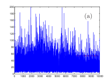
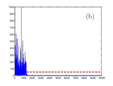
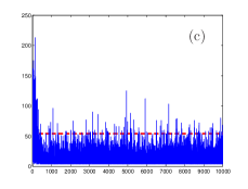
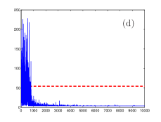
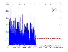
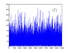
Fig. 11(f) shows for comparison the lengths of $10^{4}$ random walks through the grid of an agent whose learning has been disabled by always setting the reward to 0. The average number of 54.1 steps to reach G from S is shown in Figs. 11 and 12 as a dashed line for comparison. In Figs. 11(a-e), a positive reward of $r$ $\!=$ $\!1$ is given for hitting G. While in Fig. 11(a), the reward is always zero before G has been hit, in Fig. 11(c) hitting a boundary is punished with a negative reward of $r$ $\!=$ $\!-10$, which slightly improves the agent’s performance. [Note that all plots are specific to the respective learning rate (here $\alpha$ $\!=$ $\!10^{-1}$), which has been chosen by hand to observe an improvement within our $10^{4}$ episode-window and at the same time minimising the risk of oversized learning steps. While in general, the learning rate is gradually decreased (cf. the conditions Eq. (2.8) in Sutton and Barto (1998) to ensure convergence), this is not strictly necessary. In our numerical examples we have kept $\alpha$ constant for simplicity. Implementation of a dynamic adaptation of the learning rate as was done in Clausen et al. (2010) and Clausen (2015) in the present context is left for future work.] The transitions Fig. 11(a$\to$b) and Fig. 11(c$\to$d) show the effect of enabling gradient glow, i.e. $(\eta=1)$ $\!\to$ $\!(\eta<1)$ in (4). Gradient glow provides a mechanism of gradual backpropagation of the policy change from the nearest neighbourhood of G to cells more distant from G as the number of episodes increases. In Fig. 11, the agent settles in the optimal policy in cases (b), (d) and (e).

The policy resulting after $\!10^{4}$ episodes in case Fig. 11(d) is given in Fig. 10, where the numbers in each cell present the probability to move in the respective direction. While the agent finds the optimal policy for all cells forming the shortest path, it remains ignorant for the remaining cells. As the agent finds and consolidates the shortest path, then episode over episode, it soon visits the off-path cells less frequently, so that the transition probabilities from these cells do not accumulate enough iterations and are “frozen” in suboptimal values. This is characteristic of RL and can also be observed in learning to play games such as Backgammon Sutton and Barto (1998), where it is sufficient to play well only in typical rather than all possible constellations of the game. Since for large games, the former often form a small subset of the latter, this can be seen as a strategy to combat with large state spaces (such as number of possible game constellations). To find an optimal policy for all cells in Fig. 10, we may start each episode from a random cell, analogous to initialising the agent in an overcomplete basis as explained in Fig. 8. The red numbers in parentheses shown in Fig. 10 present a new policy obtained after $\!10^{5}$ episodes in this way. In contrast to the old policy, it is optimal or nearly optimal for all cells, with the difference between 1 and the sum of these numbers quantifying the deviation from optimality for each cell $({\scriptstyle\stackrel{{\scriptstyle<}}{{=}}}0.02)$. Since on average, the agent starts from a given cell only in 1/7-th of all episodes, the learning is slowed down, analogous to Fig. 8(a).

Fig. 12 summarises the effect of gradient glow illustrated in Fig. 11 for the two rewarding strategies.

Figure 12: Episode lengths $c$ averaged over the last 500 episodes in Fig. 11, i.e., episodes $9.5*10^{3}$ $\!-$ $\!1*10^{4}$ of single histories of individual agents in the $(3\times 3)$-grid world as shown in Fig. 10. The data points distinguish various rewarding strategies and values of gradient glow $\eta$ as explained in Fig. 11. The upper and lower dashed lines reflect a random walk and the shortest path, respectively, and the letters (a)-(f) correspond to the respective plots in Fig. 11. The optimum value of $\eta$ depends on the details of the rewarding strategy.

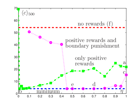
To limit the numerical effort, we have averaged the episode lengths over the last 500 episodes in Fig. 11 for individual agents as a “rule of thumb”-measure of the agent’s performance for the strategy chosen. For a deterministic calculation we must instead average the length of each episode (and for each $\eta$) over a sufficiently large ensemble of independent agents for as many episodes as needed to reach convergence. Despite these shortcomings, the results indicate a qualitatively similar behaviour as Fig. 4(a) in Melnikov et al. (2014). Figs. 11 and 12 demonstrate that gradient glow improves the agent performance, irrespective of whether or not it receives information on false intermediate moves by means of negative rewards, although the latter reduce the required length of glow. It is expected that for an ensemble average, an optimal value of $\eta$ can be found, with which the fastest convergence to the shortest path can be achieved. Fig. 11 distinguishes two qualitatively different modes of convergence. If $\eta$ is larger than optimal, a gradual improvement is observed, as seen by the damping of spikes in Fig. 11(d). If $\eta$ is smaller than optimal, then an abrupt collapse to the optimal policy without visible evidence in the preceding statistics that would provide an indication is observed, cf. Fig. 11(e). If $\eta$ is decreased further, this transition is likely to happen later, to the point it will not be observed within a fixed number of episodes. This results in the steep increase in episode length shown in Fig. 12, which would be absent if the ensemble average was used instead. This sudden transition as shown in Fig. 11(e) can also be observed for individual agents in Melnikov et al. (2014) (not shown there), which applies a softmax-policy function along with edge glow. It is surprising that the quadratic measurement-based policy simulated here exhibits the same phenomenon. Note however, that convergence does not imply optimality. In tabular RL and PS, such an abrupt transition can be observed if the $\lambda$-parameter and hence the “correlation length” is too large (in RL) or if the $\eta$-parameter is too small, so that the glow lasts too long (in PS). The policies obtained in this way are typically sub-optimal, especially in larger scale tasks such as bigger grid worlds, for which the agent learns “fast but bad” in this case. It is hence expected that a similar behaviour can be observed for our method if we increased the size of the grid.

VI Finite difference updates

This work’s numerical experiments rely on a symbolic expression (46) for the gradient $\bm{\nabla}_{t}$ in (5) for simplicity, which is usually not available in practice, also keeping in mind the variety of compositions Fig. 2, so that the agent’s memory $\hat{U}(\bm{h})$ is generally unknown. As explained in the discussion of Fig. 1, the agent may then apply a measurement-based internal loop by repeatedly preparing its memory in a state that corresponds to the last percept $s_{t}$, and register whether or how often the last measurement outcome $a_{t}$ can be recovered. This approach can be done with either infinitesimal or finite changes in the control vector $\bm{h}$, where we can distinguish between expectation value- and sample-based updates, depending on how many internal cycles are performed between consecutive external cycles. It should be stressed that the external cycles in Fig. 1 represent the agent-environment interaction, resulting in sequences of state-action pairs and corresponding rewards. While in an elementary optimal control problem, a given objective is to be optimized, here the environment poses at each external cycle a separate and generally unpredictable control problem, all of which must be addressed by the agent simultaneously.

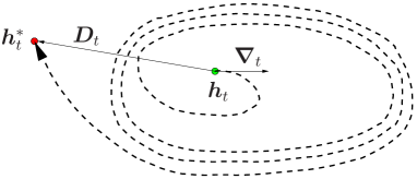
Due to the small learning rate $\alpha$, the update rule (4) is in all cases local in parameter space, which reflects the assumption, that a physical agent cannot completely reconfigure its “hardware” in a single instant. While it is then consistent to apply a gradient $\bm{D}_{t}$ $\!=$ $\!\bm{\nabla}_{t}$ as a local quantity in (4), from a computational perspective, it has a few drawbacks, however. One is that the direction of steepest accent at the current control vector $\bm{h}_{t}$ does not need to coincide with the direction $\bm{D}_{t}$ $\!=$ $\!\bm{h}_{t}^{*}$ $\!-$ $\!\bm{h}_{t}$ towards the optimum $\bm{h}_{t}^{*}$, as illustrated in Fig. 13.

Figure 13: Following the direction $\bm{\nabla}p(a_{t}|s_{t})$ of steepest ascent (dashed line) does not necessarily lead to the shortest route $\bm{D}_{t}$ $\!=$ $\!\bm{h}_{t}^{*}$ $\!-$ $\!\bm{h}_{t}$ from a given control vector $\bm{h}_{t}$ at cycle $t$ to a location $\bm{h}_{t}^{*}$, for which $p(a_{t}|s_{t})$ becomes maximum.

Another aspect is the vanishing of the gradient. Consider for example the initialisation of the action system in a mixed state (31) as done in Fig. 5(b). In particular, the graph with $p_{\mathrm{coh}}$ $\!=$ $\!0$ does not display any learning ability. Substituting the corresponding $\hat{\varrho}_{\mathrm{A}}$ $\!=$ $\!\hat{I}_{\mathrm{A}}/2$ in (31) and $\hat{U}$ $\!=$ $\!\hat{I}$ into (46), we see that the reason is the vanishing gradient, $\nabla_{k}$ $\!=$ $\!\mathrm{Im}\mathrm{Tr}[\hat{\varrho}_{\mathrm{S}}\hat{\Pi}({a})\hat{H}_{k}]$ $\!=$ $\!0$. On the other hand, the corresponding setup Fig. 6(a) reveals that in this case, substituting a SWAP-gate between S and A for $\hat{U}$ provides an optimal solution (along with an X-gate if the meaning of the symbols is reversed) for any $\hat{\varrho}_{\mathrm{A}}$, that is obviously not found in Fig. 5(b). This failure occurs despite the fact that the agents explore, as indicated by the fluctuations in Fig. 5(b). To understand the difference, note that we may generate an $\varepsilon$-greedy policy function by replacing in (6) an (arbitrarily given) state $\hat{\varrho}({s})$ with $\frac{\hat{\varrho}({s})+\varepsilon\hat{I}}{1+\varepsilon{d}}$, where $0$ $\!<$ $\!\varepsilon$ $\!\ll$ $\!1$ and $d$ $\!=$ $\!\mathrm{Tr}\hat{I}$. The term with $\hat{I}$ then gives to (6) a contribution $\sim\mathrm{Tr}_{\mathrm{A}}\hat{\Pi}({a})$, that is independent of $s$. At the same time, it does not contribute in (46) to the gradient, $\nabla_{k}$ $\!=$ $\!0$. If $\bm{D}_{t}$ $\!=$ $\!\bm{\nabla}_{t}$ $\!=$ $\!0$ for all $t$ in (4), the agent’s learning comes to rest, however. Finite difference and sample-based updates here offer a possibility to explore in parameter space the neighbourhood of the present location $\bm{h}_{t}$ (or, colloquially, the “state”) of the agent’s memory, as a consequence of asymmetries in the control landscape or statistical fluctuations in the samples.

Of particular relevance is a final fixpoint (57). Intuitively, one would assume that (despite the compactness of the (S)U($n$)-groups, that is in contrast to the potentially unbounded values of $U$ in RL or $h$ in PS) once an agent has settled in a point (57), due to the vanishing gradient, it won’t be able to react quickly, if the environment suddenly changes its allocation of rewards (without confronting the agent with percepts it has not perceived before). However, the learning curves for controllable memories (16 and 32 controls) in Fig. 7(a) demonstrate that relearning after $5\cdot 10^{3}$ cycles is not affected. A study of individual agents with 32 controls in Fig. 7(a) reveals that the Euclidean length of the numerical gradient rises from $10^{-14}$ at cycle 5000 to a value $>1$ in only 15 cycles. Better understanding of this is left for future study. In what follows, we outline the mentioned alternatives in some more detail.

VI.1 Expectation value-based updates

If the time consumed by the internal cycles is uncritical with respect to the external cycles, the agent can obtain estimates of $p(a_{t}|s_{t})$ from a sufficiently large number of internal binary measurements. With these, it can either approximate the components $\nabla_{k}p(a_{t}|s_{t};{h}_{j})$ $\!\approx$ $\![p(a_{t}|s_{t};{h}_{j}+\delta_{jk}\delta{h}_{k})$ $\!-$ $\!p(a_{t}|s_{t};{h}_{j})]/\delta{h}_{k}$ of the local gradient $\bm{\nabla}_{t}$ $\!=$ $\!\bm{\nabla}p(a_{t}|s_{t};\bm{h}_{t})$, which is then substituted as $\bm{D}_{t}$ $\!=\bm{\nabla}_{t}$ into (4). Alternatively, it can perform a global search for the location $\bm{h}_{t}^{*}$ of the maximum of $p(a_{t}|s_{t})$. A possible algorithm for the latter is differential evolution, which relies on deterministic values $p(a_{t}|s_{t};\bm{h})$ rather than noisy samples. Once an estimate for $\bm{h}_{t}^{*}$ has been found, the difference $\bm{D}_{t}$ $\!=$ $\!\bm{h}_{t}^{*}$ $\!-$ $\!\bm{h}_{t}$ is used in (4).

VI.2 Sample-based updates

Reliance on expectation values may give away potential speed gains offered by a quantum memory, which poses the question, whether a finite number of sample measurements is sufficient. Since individual updates in (4) are made with a small fraction $\alpha$ of the whole $\bm{D}_{t}$, the assumption is that the individual statistical errors in the sampled $\bm{D}_{t}$ cancel out in the long run.

As for the expectation value-based updates discussed above, samples can be used to either create discrete estimates $\nabla_{k}p(a_{t}|s_{t};{h}_{j})$ $\!\approx$ $\![s({h}_{j}+\delta_{jk}\delta{h}_{k})$ $\!-$ $\!s({h}_{j})]/2$ for the components $k$ of the local gradient $\bm{\nabla}_{t}$ $\!=$ $\!\bm{\nabla}p(a_{t}|s_{t};\bm{h}_{t})$, where $s$ $\!=$ $\!s(\bm{h}_{t})$ $\!=$ $\!\pm 1$ depending on whether the outcome of the binary measurement $(a_{t}|s_{t};\bm{h}_{t})$ is positive or not. Alternatively, for finite difference updates, one may consider a neural gas Martinetz and Schulten (1991); *Fritzke95agrowing inspired approach depicted in Fig. 14.

Figure 14: Internally generated random cloud of sample controls $\bm{h}_{k}$ around a given control vector $\bm{h}_{t}$ at cycle $t$ for which binary measurements “given $s_{t}$, detect $a_{t}$ or not” are carried out between external cycles, yielding positive ($\bm{h}_{k}^{+}$) or negative ($\bm{h}_{k}^{-}$) outcomes.

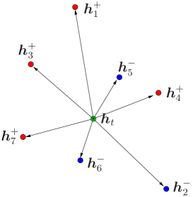
In this approach, the differences

$$\bm{D}_{t}^{(n)}=\frac{1}{n}\sum_{k=1}^{n}s_{k}\bm{h}_{k}=\frac{n-1}{n}\bm{D}_{t}^{(n-1)}+\frac{1}{n}s_{n}\bm{h}_{n}$$ (36)

between the sampled centers of positive [$s_{k}$ $\!=$ $\!s(\bm{h}_{k})$ $\!=$ $\!+1$, i.e., $\bm{h}_{k}$ $\!=$ $\!\bm{h}_{k}^{+}$] and negative outcomes ($s_{k}$ $\!=$ $\!s(\bm{h}_{k})$ $\!=$ $\!-1$, i.e., $\bm{h}_{k}$ $\!=$ $\!\bm{h}_{k}^{-}$) of the binary measurements $(a_{t}|s_{t};\bm{h}_{k})$ are then applied in (4). Although one could store a current estimate $\bm{D}_{t}^{(n)}$ for each observed state-action pair $(a_{t}|s_{t})$ and merely update it according to (36) with each new measurement point $s_{n+1}\bm{h}_{n+1}$, this would give away the generalization capability described in Sec. V.1.3. One would hence need to perform $n$ internal cycles with the POVM-based internal loop between each external cycle. The $\bm{h}_{k}$ could be drawn, e.g., from a Gaussian centered around the respective $\bm{h}_{t}$. The variance of this Gaussian could be gradually decreased with the number of external cycles to increase the locality (local resolution) of the cloud.

Fig. 13 gives the misleading impression that finite difference updates are superior to gradient-based methods. To give an illustrative counterexample, one could think of a two-dimensional $\bm{h}$ $\!=$ $\!(h_{x},h_{y})$ and a control landscape $p(\bm{h})$ modelled by the monotonically increasing height $p(l)$ along the length $l$ of a tape of paper bent into a spiral and placed onto the dashed line in Fig. 13, such that one end with $p(0)$ $\!=$ $\!0$ is located at $\bm{h}_{t}$ and the other one at $\bm{h}_{t}^{*}$. Here, a gradient-based method would safely follow the long path on the tape’s upper edge, whereas a finite difference method would trade a potential speedup with the risk of missing the paper at all trials. Since a comparison of state of the art optimal control methods based on noisy samples for the agent’s learning would go beyond the scope of this work, we here restrict ourselves to these sketchy lines of thought, whose numerical study is pending, and leave open the question of what the best method is for a given task.

A characteristic shared by the loops of Fig. 1 and optimal control setups is the need of an experimental “mastermind” who controls the controls. An agent which is supposed to act autonomously would be required to accomplish this by itself, ideally in a “natural” or “organic computing” sense. An elementary example from everyday life are “desire paths” which form or dissipate, depending on their usage and without a designated planner.

VII Summary and outlook

In summary, we have adopted an update rule from the basic PS scheme, equipped it with gradient glow, and applied it to small-scale invasion game and grid world tasks. The numerical results show that similar results can be obtained for a quantum agent, as long as the memory is not underactuated. This is not obvious, because of the fundamental difference in the number of free parameters. If $S$ and $A$ denote the number of possible percepts and actions, respectively, then in classical tabular action value RL-methods, the estimated values of all percept-action pairs are combined to a $({S}\times{A})$-matrix, i.e., we have $(SA)$ real parameters. If we encoded in our scheme each percept and action category by a separate subsystem, whose dimensionalities correspond to the number of values, the respective category can adopt, then $\hat{U}$ is an at least $U(N=SA)$-matrix for which we are faced with $(SA)^{2}$ real parameters. Note that this work is unrelated to the reflecting PS agents, which are discussed in Paparo et al. (2014). While the scheme Paparo et al. (2014) allows a proof of quantum speedup, our approach complements the latter in that it is simple, flexible in its construction, and does not involve specific analytic quantum gates. The learning of a good policy only for percepts which are “typical” and have thus been encountered sufficiently often in the past shares features with “soft computing”, where it is sufficient to find a good rather than an exact solution, which would here consist in a policy that is optimal for all possible percepts. One may think of, e.g., simplifying a symbolic mathematical expression: while all transformation steps themselves must be exact, there are no strict rules, as far as the best way of its formulation is concerned. In future work, it may be worth to incorporate recent extensions of the classical PS scheme such as generalization Melnikov et al. (2015).

Appendix A Classical PS update rule

Classical PS in its general form is based on a discrete network of clips that form its ECM. In the examples considered in Briegel and las Cuevas (2012); Mautner et al. (2015); Melnikov et al. (2014), after each discrete time step (external cycle), a local edge is updated according to

$$h_{t+1}=h_{t}-\gamma(h_{t}-h^{\mathrm{eq}})+r_{t},$$ (37)

where the instantaneous excitation $r_{t}$ $\!=$ $\!g_{t}\lambda_{t}$ is the product of the edge’s current glow value $g_{t}$ and the respective non-negative reward $\lambda_{t}$ given at this time step. The glow values dampen according to $g_{t+1}$ $\!=$ $\!(1-\eta)g_{t}$ with $g_{0}$ $\!=$ $\!0$, where $\eta\in[0,1]$ is a glow parameter, and are reset to 1 if the edge was visited during a cycle. $\gamma\in[0,1]$ is a damping parameter towards an equilibrium value $h^{\mathrm{eq}}$ in the absence of rewards (e.g., 1). Starting from some given $h_{0}$ (e.g., $h^{\mathrm{eq}}$), this gives

$$h_{t} = (1-\gamma)^{t}h_{0}+[1-(1-\gamma)^{t}]h^{\mathrm{eq}}+\sum_{k=0}^{t-1}(1-\gamma)^{k}r_{t-k-1}$$ (38)

$$= h_{0}+\sum_{k=0}^{t-1}r_{t-k-1}\quad(\gamma=0),$$

$$h_{t} \approx h^{\mathrm{eq}}+\sum_{k=0}^{t-1}(1-\gamma)^{k}r_{t-k-1}\quad(\gamma>0),$$ (39)

where the approximation as a backward-discounted sum (39) holds for times sufficiently large so that $(1-\gamma)^{t}$ $\!\ll$ $\!1$ or exactly for $h_{0}$ $\!=$ $\!h^{\mathrm{eq}}$. Note that due to the absence of damping, (38) diverges in general if $t$ grows without limit.

Appendix B Updating the memory $\hat{U}$

In App. B we focus on a model-based (i.e., symbolic) determination of the gradient $\bm{\nabla}\hat{U}(\bm{h})$. The exact form of the gradient depends on the parametrization. For example, if $\hat{U}(\bm{h})$ $\!=$ $\!\mathrm{e}^{-\mathrm{i}\hat{H}(\bm{h})}$ is given by some Hermitian $\hat{H}$, then

$$\bm{\nabla}\hat{U}=\int_{0}^{1}\mathrm{e}^{-\mathrm{i}x\hat{H}}(-\mathrm{i}\bm{\nabla}\hat{H})\mathrm{e}^{-\mathrm{i}(1-x)\hat{H}}\mathrm{d}x.$$ (40)

For small $\hat{H}$, we can expand the exponentials in $\hat{H}$ to lowest order, and the approximation $\bm{\nabla}\hat{U}$ $\!\approx$ $\!-\mathrm{i}\bm{\nabla}\hat{H}$ holds.

In case of a continuous time dependence, the vector $\bm{h}$ can be replaced by a function $h(t)$, with which a unitary propagator from time $t_{1}$ to time $t_{3}$ is given as a positively time ordered integral

$$\hat{U}(t_{3},t_{1})=\mathrm{T}\mathrm{e}^{-\mathrm{i}\int_{t_{1}}^{t_{3}}\mathrm{d}t_{2}h(t_{2})\hat{H}(t_{2})},$$ (41)

and

$$\frac{\delta\hat{U}(t,0)}{\delta{h}}(t_{1})=-\mathrm{i}\hat{U}(t,t_{1})\hat{H}(t_{1})\hat{U}(t_{1},0).$$ (42)

If $\hat{H}(t)$ $\!=$ $\!\sum_{k}\tilde{h}_{k}(t)\hat{H}_{k}$ is expanded in terms of some fixed Hamiltonians $\hat{H}_{k}$, then with $h_{k}$ $\!=$ $\!h\tilde{h}_{k}$, (41) becomes $\hat{U}(t_{3},t_{1})$ $\!=$ $\!\mathrm{T}\mathrm{e}^{-\mathrm{i}\int_{t_{1}}^{t_{3}}\mathrm{d}t_{2}\sum_{k}h_{k}(t_{2})\hat{H}_{k}}$, and (42) is replaced with $\frac{\delta\hat{U}(t,0)}{\delta{h_{k}}}(t_{1})$ $\!=$ $\!-\mathrm{i}\hat{U}(t,t_{1})\hat{H}_{k}\hat{U}(t_{1},0)$. Navigation on unitary groups becomes discretized if only a restricted (finite) set of Hamiltonians $\hat{H}_{k}$ can be implemented at a time rather than an analytically time-dependent Hamiltonian $\hat{H}(t)$, so that only one of the $\tilde{h}_{k}$ is non-zero for a given $t$. A known example is the alternating application of two fixed Hamiltonians Lloyd (1995), $\hat{H}_{2k}$ $\!=$ $\!\hat{H}^{(2)}$ and $\hat{H}_{2k+1}$ $\!=$ $\!\hat{H}^{(1)}$ $(k=0,1,2,\ldots,\lfloor\frac{n}{2}\rfloor)$, for a set of times to be determined from the target unitary Harel and Akulin (1999). In this discrete case as defined by a piecewise constant normalized $\hat{H}$ in (41), the function $h(t)$ can be replaced with a vector $\bm{h}$, and the functional derivatives with respect to $h(t)$ reduce to gradients with respect to $\bm{h}$.

B.1 Adding layer after layer

We can update the present unitary $\hat{U}$ by multiplying it from the left with a new layer $\hat{U}(\delta\bm{h})$ after each cycle,

$$\hat{U}\leftarrow\hat{U}(\delta\bm{h})\hat{U}.$$ (43)

If $\hat{U}(\delta\bm{h})$ $\!=$ $\!\mathrm{e}^{-\mathrm{i}\sum_{k}\delta{h}_{k}\hat{H}_{k}}$ is a small modification close to the identity, then the mentioned approximation of (40) gives $(\bm{\nabla}\hat{U})_{k}$ $\!\approx$ $\!-\mathrm{i}\hat{H}_{k}\hat{U}$. This is of advantage if the agent or its simulation is able to store only the present $\hat{U}$ and not the history of updates (layers). The components of (5) then become

$$\frac{\partial{p}({a}|{s})}{\partial{h}_{k}}=2\mathrm{Im}\bigl{\langle}\hat{U}^{\dagger}\hat{\Pi}({a})\hat{H}_{k}\hat{U}\bigr{\rangle}.$$ (44)

B.2 Fixed number of layers

In our numerical examples we consider a discretized memory model, for which (41) reduces to a product of $n$ unitaries

$$\hat{U}=\hat{U}_{n}\cdots\hat{U}_{2}\hat{U}_{1},\quad\hat{U}_{k}=\mathrm{e}^{-\mathrm{i}{h}_{k}\hat{H}_{k}},$$ (45)

which simplifies the determination of the gradient, since $(\bm{\nabla}\hat{U})_{k}$ $\!=$ $\!-\mathrm{i}\hat{U}\hat{H}_{k}(t_{k})$, where $\hat{H}_{k}(t_{k})$ $\!=$ $\!(\hat{U}_{k}\cdots\hat{U}_{1})^{\dagger}\hat{H}_{k}(\hat{U}_{k}\cdots\hat{U}_{1})$, so that the components of (5) now become

$$\frac{\partial{p}({a}|{s})}{\partial{h}_{k}}=2\mathrm{Im}\bigl{\langle}\hat{U}^{\dagger}\hat{\Pi}({a})\hat{U}\hat{H}_{k}(t_{k})\bigr{\rangle}.$$ (46)

In this work, we use alternating layers defined by two fixed Hamiltonians $\hat{H}^{(1)}$ and $\hat{H}^{(2)}$ as mentioned at the beginning of this section.

Appendix C Numerical and measurement-based objectives

C.1 Distance and uniformly averaged fidelity

Consider an $n$-level system and two unitary operators $\hat{U}$ and $\hat{U}_{\mathrm{T}}$, where $\hat{U}$ $\!=$ $\!\hat{U}({h})$ depends on an (unrestricted) external control field $h(t)$, and $\!\hat{U}_{\mathrm{T}}$ is a desired target. Their (squared) Euclidean distance as induced by the Hilbert-Schmidt dot product is given by

$$D \equiv \|\hat{U}-\hat{U}_{\mathrm{T}}\|^{2}=\mathrm{Tr}\bigl{[}(\hat{U}-\hat{U}_{\mathrm{T}})^{\dagger}(\hat{U}-\hat{U}_{\mathrm{T}})\bigr{]}$$ (47)

$$= 2n-2\mathrm{Re}\mathrm{Tr}(\hat{U}_{\mathrm{T}}^{\dagger}\hat{U})\in[0,4n].$$

If $\hat{U}({h})$ is controllable in the sense that at least one $h(t)$ exists such that $\hat{U}({h})$ $\!=$ $\!\hat{U}_{\mathrm{T}}$, then (47) has the set $\{0,4,\ldots,4n\}$ as possible extremal values (i.e, $\frac{\delta{D}}{\delta{h}}$ $\!=$ $\!0$), where the values $0$ and $4n$ are attained for $\hat{U}$ $\!=$ $\!\pm\hat{U}_{\mathrm{T}}$, while the remaining extrema are saddle points Rabitz et al. (2005). A measure insensitive to global phases $\hat{U}$ $\!=$ $\!\mathrm{e}^{\mathrm{i}\varphi}\hat{U}_{\mathrm{T}}$ is the average fidelity defined by

$$F\equiv\overline{|\langle\Psi|\hat{U}_{\mathrm{T}}^{\dagger}\hat{U}|\Psi\rangle|^{2}}=\frac{n+|\mathrm{Tr}(\hat{U}_{\mathrm{T}}^{\dagger}\hat{U})|^{2}}{n(n+1)},$$ (48)

where the overline denotes uniform average over all $|\Psi\rangle$ Pedersen et al. (2007); Dankert (2005). Note that $F$ $\!\in$ $\![(n+1)^{-1},1]$ for $n$ $\!>$ $\!1$, and $F$ $\!=$ $\!1$ for $n$ $\!=$ $\!1$. Both (47) and (48) are determined by the complex

$$\cos\sphericalangle\bigl{(}\hat{U},\hat{U}_{\mathrm{T}}\bigr{)}\equiv\frac{\mathrm{Tr}(\hat{U}_{\mathrm{T}}^{\dagger}\hat{U})}{\sqrt{\mathrm{Tr}(\hat{U}^{\dagger}\hat{U})}\sqrt{\mathrm{Tr}(\hat{U}_{\mathrm{T}}^{\dagger}\hat{U}_{\mathrm{T}})}}=\frac{\mathrm{Tr}(\hat{U}_{\mathrm{T}}^{\dagger}\hat{U})}{n},$$ (49)

which is confined to the complex unit circle and whose expectation $\bigl{\langle}|\cos\sphericalangle(\hat{U},\hat{U}_{\mathrm{T}})|^{2}\bigr{\rangle}$ $\!=$ $\!n^{-1}$ for uniform random $\hat{U}$ drops to zero with growing $n$.

If in (48), the averaging is restricted to a $d$-dimensional subspace P, we must replace (48) with

$$F_{\mathrm{P}}\equiv\overline{|\langle\Psi|\hat{M}|\Psi\rangle|^{2}}^{(\mathrm{P})}=\frac{\mathrm{Tr}(\hat{M}^{\dagger}\hat{M})+|\mathrm{Tr}(\hat{M})|^{2}}{d(d+1)},$$ (50)

where $\hat{M}$ $\!=$ $\!\hat{P}\hat{U}_{\mathrm{T}}^{\dagger}\hat{U}\hat{P}$, with $\hat{P}$ being the projector onto P. Note that $F_{\mathrm{P}}$ $\!\in$ $\![\frac{\max(0,2d-n)}{d(d+1)},1]$ for $n$ $\!>$ $\!1$ [since $\mathrm{Tr}(\hat{M}^{\dagger}\hat{M})$ $\!=$ $\!\mathrm{Tr}(\hat{P}_{\mathrm{T}}\hat{P}_{\mathrm{U}})$ $\!\in$ $\!\max(0,2d-n)$ with $\hat{P}_{\mathrm{T}}$ $\!=$ $\!\hat{U}_{\mathrm{T}}\hat{P}\hat{U}_{\mathrm{T}}^{\dagger}$, $\hat{P}_{\mathrm{U}}$ $\!=$ $\!\hat{U}\hat{P}\hat{U}^{\dagger}$], and $F_{\mathrm{P}}$ $\!=$ $\!1$ for $n$ $\!=$ $\!1$. While for a one-dimensional $\hat{P}$ $\!=$ $\!|\Psi\rangle\langle\Psi|$, (50) reduces to $F_{\Psi}$ $\!=$ $\!|\langle\Psi|\hat{U}_{\mathrm{T}}^{\dagger}\hat{U}|\Psi\rangle|^{2}$, the other limit $d$ $\!=$ $\!n$ recovers (48).

If in (50), $\hat{U}$ $\!=$ $\!\hat{U}_{\mathrm{SB}}$ couples the quantum system S to a bath B, then we define a projector $\hat{\Pi}$ $\!=$ $\!\hat{U}_{\mathrm{T}}\hat{P}|\Psi\rangle\langle\Psi|\hat{P}\hat{U}_{\mathrm{T}}^{\dagger}\otimes\hat{I}_{\mathrm{B}}$ and generalize (50) to

$$F_{\mathrm{P}} \equiv \overline{\mathrm{Tr}_{\mathrm{SB}}\bigl{[}\hat{U}\hat{P}|\Psi\rangle\hat{\varrho}_{\mathrm{B}}\langle\Psi|\hat{P}\hat{U}^{\dagger}\hat{\Pi}\bigr{]}}^{(\mathrm{P})}$$ (51)

$$= \left\langle\frac{\mathrm{Tr}_{\mathrm{S}}(\hat{M}^{\dagger}\hat{M})+(\mathrm{Tr}_{\mathrm{S}}\hat{M})^{\dagger}(\mathrm{Tr}_{\mathrm{S}}\hat{M})}{d(d+1)}\right\rangle_{\mathrm{B}},$$ (52)

where $\langle\cdots\rangle_{\mathrm{B}}$ $\!\equiv$ $\!\mathrm{Tr}_{\mathrm{B}}[\hat{\varrho}_{\mathrm{B}}(\cdots)]$ with a fixed bath state $\hat{\varrho}_{\mathrm{B}}$.

Replacing $\hat{U}|\Psi\rangle\langle\Psi|\hat{U}^{\dagger}$ in (48) with the output $\mathcal{M}(|\Psi\rangle\langle\Psi|)$ of a quantum channel generalizes (48) to Pedersen et al. (2007)

$$F=\overline{\langle\Psi|\hat{U}_{\mathrm{T}}^{\dagger}\mathcal{M}(|\Psi\rangle\langle\Psi|)\hat{U}_{\mathrm{T}}|\Psi\rangle}=\frac{n+\sum_{k}|\mathrm{Tr}(\hat{U}_{\mathrm{T}}^{\dagger}\hat{G}_{k})|^{2}}{n(n+1)},$$ (53)

where $\hat{G}_{k}$ are the Kraus operators of the decomposition of the channel map $\mathcal{M}(\hat{\varrho})$ $\!=$ $\!\sum_{k}\hat{G}_{k}\hat{\varrho}\hat{G}_{k}^{\dagger}$. Note that a change $\hat{G}_{k}^{\prime}$ $\!=$ $\!\sum_{j}V_{kj}\hat{G}_{j}$ of the Kraus operators as described by a unitary matrix $V$ leaves (53) invariant.

C.2 Percept statistics-based fidelity

The uniform average in (53) can be generalized to an arbitrary distribution ${p}(|\Psi_{k}\rangle)$ of possible input states $|\Psi_{k}\rangle$,

$$\hat{\varrho}_{\mathrm{in}}=\sum_{k}{p}(|\Psi_{k}\rangle)|\Psi_{k}\rangle\langle\Psi_{k}|,$$ (54)

that reflects the statistics of their occurrence in different instances of applications of the device (external cycles in a control loop). This generalizes (53) to

$$F_{\hat{\varrho}_{\mathrm{in}}}\equiv{p}(\hat{U}_{\mathrm{T}})=\sum_{k}{p}(\hat{U}_{\mathrm{T}}||\Psi_{k}\rangle){p}(|\Psi_{k}\rangle),$$ (55)

$${p}(\hat{U}_{\mathrm{T}}||\Psi_{k}\rangle)=\langle\Psi_{k}|\hat{U}_{\mathrm{T}}^{\dagger}\mathcal{M}(|\Psi_{k}\rangle\langle\Psi_{k}|)\hat{U}_{\mathrm{T}}|\Psi_{k}\rangle,\quad$$ (56)

which is just the total probability ${p}(\hat{U}_{\mathrm{T}})$ of correctly detecting a $\hat{U}_{\mathrm{T}}$-transformed pure (but unknown) input state drawn from a distribution (54). Once $p(\hat{U}_{\mathrm{T}})$ $\!=$ $\!1$, the channel’s effect is indistinguishable from that of $\hat{U}_{\mathrm{T}}$ for the set of possible inputs $|\Psi_{k}\rangle$, (i.e. those for which ${p}(|\Psi_{k}\rangle)$ $\!>$ $\!0$). The case $p(\hat{U}_{\mathrm{T}})$ $\!\scriptstyle{\stackrel{{\scriptstyle<}}{{\approx}}}$ $\!1$ is relevant from a numerical and experimental point of view. Rare inputs $|\Psi_{k}\rangle$, for which $0$ $\!<$ $\!{p}(|\Psi_{k}\rangle)$ $\!\ll$ $\!1$, will hardly affect $p(\hat{U}_{\mathrm{T}})$ in a control loop, which relaxes the demands on the channel compared to the uniform average (53). The channel optimization itself is thus economized in the sense that it is required to perform well only on typical rather than all inputs.

Here, we consider a navigation of $\hat{U}$ in the above-mentioned discretized case, $\hat{U}$ $\!=$ $\!\hat{U}(\bm{h})$, that starts at the identity $\hat{U}(\bm{h}$ $\!=$ $\!\bm{0})$ $\!=$ $\!\hat{I}$ and from there undertakes a gradient-based maximization of ${p}(\hat{U}_{\mathrm{T}})$ as defined in (55) to a point where

$$\bm{\nabla}{p}(\hat{U}_{\mathrm{T}})=0.$$ (57)

The control vector $\bm{h}$ typically represents system variables and not those of the bath. Rather than solving for the parameters Harel and Akulin (1999) for which the scheme Lloyd (1995) yields a desired given unitary, we search parameters, for which the unitary, whose specific form we are not interested in, solves a given task.

C.3 Optimal memory navigation and constrained optimization

While here we have discussed and compared concrete types of algorithms, a more fundamental question concerns the optimality and derivation of general (e.g., speed) limits of the learning process. Although the physical time is given as the sum of the agent and environment response times over each cycle, one may restrict to counting the number of (a) memory cycles in total, (b) external cycles only (c) episodes or (d) parameter updates $\delta\bm{h}$ of the memory $\hat{U}(\bm{h})$, depending on what the most critical criterion is. Not only should the navigation of $\hat{U}$ from the identity to a point (57) follow an optimal trajectory, but also the navigation of the percept states by a given $\hat{U}$ should be such that the individual physical memory evolution times become minimum. Such demands may conflict with restrictions on the practical implementability and complexity of the memory. Since these questions are beyond the scope of this work, in what follows we restrict ourselves to outline a connection to constrained optimisation as a possible formal approach.

Assuming the Schrödinger equation $\frac{\mathrm{d}}{\mathrm{d}t}\hat{U}$ $\!=$ $\!-\mathrm{i}\hat{H}\hat{U}$ and a fixed energy-type constraint $\|\frac{\mathrm{d}}{\mathrm{d}t}\hat{U}\|^{2}$ $\!=$ $\!\mathrm{Tr}(\hat{H}^{2})$ $\!\scriptstyle{\stackrel{{\scriptstyle!}}{{=}}}$ $\!E^{2}$, the length of a curve in the space of unitaries becomes

$$L=\int_{0}^{T}\Bigl{\|}\frac{\mathrm{d}\hat{U}}{\mathrm{d}t}\Bigr{\|}\mathrm{d}t\stackrel{{\scriptstyle!}}{{=}}ET,$$ (58)

where T is the arrival (or protocol) time, $\hat{U}(t=T)$ $\!=$ $\!\hat{U}_{\mathrm{T}}$ Russell and Stepney (2014); Wang et al. (2015). (A “protocol” refers to a prescription for the time dependence of ${h}$, $\hat{H}$, or $\hat{U}$.) In addition to (or instead of) the protocol time $T$, we may also consider

$$C\equiv\int_{0}^{T}\Bigl{\|}\frac{\mathrm{d}\hat{H}}{\mathrm{d}t}\Bigr{\|}\mathrm{d}t$$ (59)

as a measure of the complexity of the protocol that integrates the changes that have to be made on $\hat{H}$ via the control fields.

If the optimization problem comprises two objectives such as minimising a distance $D$ or maximising a fidelity $F$ with minimum amount of (58) or (59), then an approximate approach consists in first finding an $h(t)$ that optimizes an objective function $J_{1}$ under a fixed constraint $J_{2}$. Here, $J_{1}$ represents $D$ or $F$, while $J_{2}$ may represent $L$ or $C$. This can be formulated as an Euler-Lagrange equation

$$\frac{\delta{J_{1}}}{\delta{h}}-\lambda\frac{\delta{J_{2}}}{\delta{h}}=0,$$ (60)

where the Lagrange multiplier $\lambda$ must finally be substituted with the given constant such as $L$ or $C$. This optimisation is then repeated with stepwise decreased $L$ or $C$, until the deterioration of the achievable $J_{1}$ exceeds a certain threshold. Equivalently, (60) may also be thought of optimizing $J_{2}$ under the constraint of constant $J_{1}$. Eq. (60), which contains both derivatives in a symmetric way, merely states the linear dependence of the functional derivatives at an extremal point ${h}$ in the function space $\{h\}$.

In the discrete case, the time integrals in Eqs. (58) and (59) reduce to sums over time intervals with constant $\hat{H}$, and in (59) we assume that each jump of $\hat{H}$ gives a fixed finite contribution. To gain some intuition into the meaning of $C$, we may think of navigating through a classical rectangular grid. There is a set of shortest paths connecting the diagonal corners, but they are not equivalent with respect to the number of turns the navigator has to make along its way. In the quantum context, the number of switches equals the number of intervals with constant $\hat{H}$, which may be thought of “gates”. In contrast to an analytical design of quantum circuits, the circuit is here generated numerically, however. Since each switch to a different $\hat{H}$ changes the instantaneous eigenbasis, we may thus think rather of “layers” drawing an analogy to classical artificial neural networks Rojas (1996).