h SLAC-PUB-16330
h TTK–16–03
Simplified Models for Higgs Physics: Singlet Scalar and Vector-like Quark Phenomenology

Matthew J. Dolan1111E-mail: dolan@unimelb.edu.au,  J.L. Hewett2222E-mail: hewett@slac.stanford.edu,  M. Krämer3333E-mail: mkraemer@physik.rwth-aachen.de, and T.G. Rizzo2444E-mail: rizzo@slac.stanford.edu
1ARC Centre of Excellence for Particle Physics at the Terascale,
School of Physics, University of Melbourne, 3010, Australia
2 SLAC National Accelerator Laboratory, Menlo Park 94025, CA, USA
3Institute for Theoretical Particle Physics and Cosmology,
RWTH Aachen University, D-52056 Aachen, Germany
Abstract

Simplified models provide a useful tool to conduct the search and exploration of physics beyond the Standard Model in a model-independent fashion. In this work we consider the complementarity of indirect searches for new physics in Higgs couplings and distributions with direct searches for new particles, using a simplified model which includes a new singlet scalar resonance and vector-like fermions that can mix with the SM top-quark. We fit this model to the combined ATLAS and CMS 125 GeV Higgs production and coupling measurements and other precision electroweak constraints, and explore in detail the effects of the new matter content upon Higgs production and kinematics. We highlight some novel features and decay modes of the top partner phenomenology, and discuss prospects for Run II.

1 Introduction

Two of the main objectives of the Large Hadron Collider (LHC) Run II are studying the detailed spectroscopy of the Higgs boson and continuing the search for physics Beyond the Standard Model (BSM). The properties of the recently discovered 125 GeV Higgs boson provide a new tool in the search for new physics and may indirectly reveal its existence, whereas the gain in the center-of-mass energy of the collider in Run II supplies fertile ground to directly discover new particles.

The majority of searches for new physics at the LHC are now designed and interpreted in terms of Simplified Models [1, 2]. Simplified Models provide a framework for understanding the broad kinematic features of signatures using a small number of parameters, such as masses and couplings of new fields, without depending on specific characteristics of full UV-complete models. This focus on the relevant weak scale Lagrangian parameters allows for the design of relatively model-independent BSM searches that are broadly applicable to new physics scenarios. Due to these advantages, the simplified model approach has recently been extended to searches for dark matter particles at the LHC [3, 4, 5, 6, 7].

The use of simplified models is not restricted to new physics searches, as they can also be of utility in understanding the limits set on new physics from precision Standard Model (SM) measurements such as the properties of the Higgs boson. Another approach often employed in this context is Effective Field Theory (EFT), where constraints are set on the Wilson coefficients of higher dimensional operators constructed out of Standard Model fields. A UV-complete theory can be mapped onto the EFT by integrating out the new heavy states, assuming there is a hierarchy of scales between the SM and new states. Simplified models differ in allowing the direct exploration of the phenomenology of the BSM states.

The purpose of this paper is to develop the simplified model approach for Higgs physics and investigate the interplay between the various approaches. We set up a framework to explore BSM theories that affect the Higgs sector and connect measurements of Higgs properties with direct searches for new physics.

To do this we construct a class of simplified models that introduce modifications to the Higgs couplings to SM fields, but which are also amenable to direct searches at the LHC. In particular, we study an extension of the SM that involves a scalar singlet as well as vector-like fermions which mix with the top quark. We argue that such models assist in the exploration of the space of BSM theories that could affect the properties of the Higgs. Models with this matter content are of interest since singlet scalars can be identified with Higgs portal models [8, 9, 10] and vector-like partners of the top-quark appear in numerous BSM scenarios, including composite Higgs models, warped extra dimensions, Little Higgs and extended grand unified theories. In particular, the presence of a singlet in association with the vector-like quarks is also known to help stabilize the electroweak vacuum [11, 12].

This scenario leads to calculable changes in the couplings of the SM-like 125 GeV Higgs boson, which we constrain using the combined ATLAS and CMS measurements of the Higgs production cross-sections and branching ratios, as well as other electroweak precision data.

As well as serving as a framework that illuminates the effects of precision Higgs measurements on extended scalar sectors, this simplified model is useful for exploring vector-like quark phenomenology. The presence of the singlet leads to new top partner decay channels, a fact which has also been noticed in the context of composite Higgs models [13, 14]. There are also a variety of direct searches for the top partners, such as single top-partner production [15, 16], which we discuss in detail below.

Ultimately we find that the EFT and simplified model approaches are complementary. Precision Higgs (and electroweak) measurements set constraints on the parameter space of the simplified model, and in turn inform the collider phenomenology of the new particles555A similar model has been studied in this context in [17].. The constraints on this perturbative simplified model are found to be compatible with the EFT approach [18]. We show that given the constraints from direct searches that it is unlikely for there to be large effects on Higgs differential distributions, even when the momentum and mass dependence of top-partners running in loops is correctly taken into account.

Recently there has been much interest in a possible diphoton resonance signal at 750 GeV as observed by ATLAS and CMS in the initial few femtobarns data of Run 2 [19, 20]. Among other possibilities, a number of analyses have appeared suggesting this may be due to a similar class of models to the one we study here involving singlet scalars and vector-like fermions [21, 22, 23, 24, 25, 26, 27, 28, 29]. While this further motivates our study, we note that for vector-like top partners the required diphoton signal strength can only be achieved for non-perturbative values of the couplings, unless multiple families of top-partners are present.

The structure of the paper is as follows: In Section 2 we introduce and discuss the details of our model, after which we present the indirect constraints from Run I Higgs measurements in Section 3. In Section 4 we study the singlet scalar phenomenology as well as effects of our model on differential Higgs distributions. We then focus on the vector-like quark phenomenology in Section 5, discussing current bounds and suggesting new directions to be taken in Run II, after which we conclude. Some technical details are contained in the Appendix.

2 A Simplified Model

In constructing a first simplified model for Higgs physics, we examine a scenario with minimal particle content and interactions that influences the 125 GeV Higgs couplings in a calculable manner. We thus choose to add two ingredients to the SM: (i𝑖i) a scalar singlet S𝑆S, and (ii𝑖𝑖ii) a vector-like fermion F𝐹F. The singlet S𝑆S acquires a vev, S=(s+vS)𝑆𝑠subscript𝑣𝑆S=(s+v_{S}), and provides mass for the vector-like fermion, mF=yFvSsubscript𝑚𝐹subscript𝑦𝐹subscript𝑣𝑆m_{F}=y_{F}v_{S}. The Higgs and new scalar fields mix via the term λHSHHS2subscript𝜆𝐻𝑆superscript𝐻𝐻superscript𝑆2\lambda_{HS}H^{\dagger}HS^{2}, and thus generate new physics effects in both the gauge and fermionic SM Higgs couplings. Various choices for the quantum numbers of F𝐹F are possible, and different representations result in specific patterns for the Higgs cross sections and couplings. These are outlined in Table 1 for the Higgs gauge boson couplings hVμνVμνsubscript𝑉𝜇𝜈superscript𝑉𝜇𝜈hV_{\mu\nu}V^{\mu\nu} induced by the vector-like fermion F𝐹F. The gauge couplings are defined in terms of the coefficients ϵVsubscriptitalic-ϵ𝑉\epsilon_{V} as

γγ:ϵγαπ1vH(λHSvH2mS2),:𝛾𝛾subscriptitalic-ϵ𝛾𝛼𝜋1subscript𝑣𝐻subscript𝜆𝐻𝑆superscriptsubscript𝑣𝐻2superscriptsubscript𝑚𝑆2\displaystyle\gamma\gamma:\,\,\epsilon_{\gamma}{\alpha\over\pi}{1\over v_{H}}\Big{(}{\lambda_{HS}v_{H}^{2}\over m_{S}^{2}}\Big{)}\,, GaGa:ϵgαsπ1vH(λHSvH2mS2),:subscript𝐺𝑎superscript𝐺𝑎subscriptitalic-ϵ𝑔subscript𝛼𝑠𝜋1subscript𝑣𝐻subscript𝜆𝐻𝑆superscriptsubscript𝑣𝐻2superscriptsubscript𝑚𝑆2\displaystyle G_{a}G^{a}:\,\,\epsilon_{g}{\alpha_{s}\over\pi}{1\over v_{H}}\Big{(}{\lambda_{HS}v_{H}^{2}\over m_{S}^{2}}\Big{)}\,,
BB:ϵBg2π21vH(λHSvH2mS2),:𝐵𝐵subscriptitalic-ϵ𝐵superscript𝑔2superscript𝜋21subscript𝑣𝐻subscript𝜆𝐻𝑆superscriptsubscript𝑣𝐻2superscriptsubscript𝑚𝑆2\displaystyle BB:\,\,\epsilon_{B}{g^{\prime 2}\over\pi^{2}}{1\over v_{H}}\Big{(}{\lambda_{HS}v_{H}^{2}\over m_{S}^{2}}\Big{)}\,, WiWi:ϵWg2π21vH(λHSvH2mS2),:subscript𝑊𝑖superscript𝑊𝑖subscriptitalic-ϵ𝑊superscript𝑔2superscript𝜋21subscript𝑣𝐻subscript𝜆𝐻𝑆superscriptsubscript𝑣𝐻2superscriptsubscript𝑚𝑆2\displaystyle W_{i}W^{i}:\,\,\epsilon_{W}{g^{2}\over\pi^{2}}{1\over v_{H}}\Big{(}{\lambda_{HS}v_{H}^{2}\over m_{S}^{2}}\Big{)}\,, (1)

and the ϵVsubscriptitalic-ϵ𝑉\epsilon_{V} take on values as determined by the F𝐹F representation. Here, vHsubscript𝑣𝐻v_{H} is the vaccum expectation value of the SM-like Higgs field H𝐻H.

F ϵγsubscriptitalic-ϵ𝛾\epsilon_{\gamma} ϵgsubscriptitalic-ϵ𝑔\epsilon_{g} ϵBsubscriptitalic-ϵ𝐵\epsilon_{B} ϵWsubscriptitalic-ϵ𝑊\epsilon_{W}
(TB)L+Rsubscriptsuperscript𝑇superscript𝐵𝐿𝑅\left(\begin{array}[]{c}T^{\prime}\\ B^{\prime}\end{array}\right)_{L+R} 518518{5\over 18} 1616-{1\over 6} 11441144{1\over 144} 116116{1\over 16}
QL+Rsubscript𝑄𝐿𝑅Q_{L+R} 12Q212superscript𝑄2{1\over 2}Q^{2} 112112-{1\over 12} 18Q218superscript𝑄2{1\over 8}Q^{2} 0
(NE)L+Rsubscript𝑁𝐸𝐿𝑅\left(\begin{array}[]{c}N\\ E\end{array}\right)_{L+R} 1616{1\over 6} 0 148148{1\over 48} 148148{1\over 48}
LL+Rsubscript𝐿𝐿𝑅L_{L+R} 116Q2116superscript𝑄2{1\over 16}Q^{2} 0 124124{1\over 24} 0
Table 1: Possible vector-like fermion representations and their influence on the Higgs couplings to gauge fields. Q2superscript𝑄2Q^{2} represents the square of the fermion’s electric charge and ϵVsubscriptitalic-ϵ𝑉\epsilon_{V} is the derived coefficient of the hVμνVμνsubscript𝑉𝜇𝜈superscript𝑉𝜇𝜈hV_{\mu\nu}V^{\mu\nu} operator.

In this paper, for simplicity, we consider the case where F𝐹F is a color-triplet and SU(2) singlet vector-like fermion field, T𝑇T, with charge QF=+2/3subscript𝑄𝐹23Q_{F}=+2/3. We assume that the vector-like fermion mixes with the SM top-quark only. This model was chosen such that in the heavy particle limit it introduces all the (CP-even) dimension-6 operators that affect Higgs physics and are not severely constrained by electroweak precision physics. Such a model has also been considered in [11] in the context of stabilizing the electroweak vacuum in the presence of new vector-like fermion representations. We intend on returning to the other possibilities, some of which have been garnering interest recently in the context of the 750 GeV diphoton excess, in future publications.

The most general Lagrangian for our model includes new Yukawa and gauge terms for the SM top-quark and the new vector fermion, as well as an extended scalar potential:

Yukawa+gaugeV(H,S).subscriptYukawasubscriptgauge𝑉𝐻𝑆\mathcal{L}\supset\mathcal{L}_{\rm Yukawa}+\mathcal{L}_{\rm gauge}-V(H,S). (2)

We discuss the various new contributions in Eq.(2) in turn below.

The Yukawa interactions

The most general fermion mass terms for the SM top-quark and the vector-like fermion T𝑇T are

Yukawa=yTST¯LintTRint+λ~ST¯LinttRintsubscriptYukawasubscript𝑦𝑇𝑆subscriptsuperscript¯𝑇int𝐿subscriptsuperscript𝑇int𝑅~𝜆𝑆subscriptsuperscript¯𝑇int𝐿subscriptsuperscript𝑡int𝑅\displaystyle\mathcal{L}_{\rm Yukawa}=y_{T}S\overline{T}^{\rm int}_{L}T^{\rm int}_{R}+\tilde{\lambda}S\overline{T}^{\rm int}_{L}t^{\rm int}_{R}
+ytQ¯LintH~tRint+ybQ¯LintHbR+λTQ¯LintH~TRint+mDT¯LintTRint,subscript𝑦𝑡subscriptsuperscript¯𝑄int𝐿~𝐻subscriptsuperscript𝑡int𝑅subscript𝑦𝑏subscriptsuperscript¯𝑄int𝐿𝐻subscript𝑏𝑅subscript𝜆𝑇subscriptsuperscript¯𝑄int𝐿~𝐻subscriptsuperscript𝑇int𝑅subscript𝑚𝐷subscriptsuperscript¯𝑇int𝐿subscriptsuperscript𝑇int𝑅\displaystyle\qquad+y_{t}\overline{Q}^{\rm int}_{L}\widetilde{H}t^{\rm int}_{R}+y_{b}\overline{Q}^{\rm int}_{L}Hb_{R}+\lambda_{T}\overline{Q}^{\rm int}_{L}\widetilde{H}T^{\rm int}_{R}+m_{D}\overline{T}^{\rm int}_{L}T^{\rm int}_{R},

where H~=iσ2H~𝐻𝑖subscript𝜎2superscript𝐻\widetilde{H}=i\sigma_{2}H^{*}, Q¯Lint=(t¯Lintb¯Lint)subscriptsuperscript¯𝑄int𝐿subscriptsuperscript¯𝑡int𝐿subscriptsuperscript¯𝑏int𝐿\overline{Q}^{\rm int}_{L}=(\bar{t}^{\rm int}_{L}\;\bar{b}^{\rm int}_{L}), and ψL,R=12(1γ5)ψsubscript𝜓𝐿𝑅12minus-or-plus1subscript𝛾5𝜓\psi_{L,R}=\frac{1}{2}(1\mp\gamma_{5})\psi. We denote the weak interaction eigenstates by tintsuperscript𝑡intt^{\rm int} and Tintsuperscript𝑇intT^{\rm int}, while t𝑡t and T𝑇T are used for the mass eigenstates.

Through a rotation of the fields (tRint,TRint)subscriptsuperscript𝑡int𝑅subscriptsuperscript𝑇int𝑅(t^{\rm int}_{R},T^{\rm int}_{R}) one can remove the term proportional to T¯LinttRintsubscriptsuperscript¯𝑇int𝐿subscriptsuperscript𝑡int𝑅\overline{T}^{\rm int}_{L}t^{\rm int}_{R}. Furthermore, to reduce the number of free parameters, we assume that the mass of the vector fermion is generated from the vev of the singlet field only and set mD=0subscript𝑚𝐷0m_{D}=0. We thus have

Yukawa=yTST¯LintTRint+ytQ¯LintH~tRint+ybQ¯LintHbR+λTQ¯LintH~TRint.subscriptYukawasubscript𝑦𝑇𝑆subscriptsuperscript¯𝑇int𝐿subscriptsuperscript𝑇int𝑅subscript𝑦𝑡subscriptsuperscript¯𝑄int𝐿~𝐻subscriptsuperscript𝑡int𝑅subscript𝑦𝑏subscriptsuperscript¯𝑄int𝐿𝐻subscript𝑏𝑅subscript𝜆𝑇subscriptsuperscript¯𝑄int𝐿~𝐻subscriptsuperscript𝑇int𝑅{\mathcal{L}_{\rm Yukawa}=y_{T}S\overline{T}^{\rm int}_{L}T^{\rm int}_{R}+y_{t}\overline{Q}^{\rm int}_{L}\widetilde{H}t^{\rm int}_{R}+y_{b}\overline{Q}^{\rm int}_{L}Hb_{R}+\lambda_{T}\overline{Q}^{\rm int}_{L}\widetilde{H}T^{\rm int}_{R}.} (4)

After spontaneous symmetry breaking, the SM top-quark tintsuperscript𝑡intt^{\rm int} and the vector quark Tintsuperscript𝑇intT^{\rm int} mix to form the mass eigenstates. We provide the explicit forms for these mixings in Appendix A.2.

Gauge interactions of the vector-like fermion

The vector-like fermion field Tintsuperscript𝑇intT^{\rm int} carries the quantum numbers hypercharge YT=4/3subscript𝑌𝑇43Y_{T}=4/3 and electromagnetic charge QT=2/3subscript𝑄𝑇23Q_{T}=2/3. The terms in the Lagrangian involving the vector-like fermion T𝑇T and the SM third generation quarks t,b𝑡𝑏t,b are:

gaugesubscriptgauge\displaystyle\mathcal{L}_{\rm gauge} it¯∂̸t+iT¯∂̸T+ib¯∂̸b𝑖¯𝑡not-partial-differential𝑡𝑖¯𝑇not-partial-differential𝑇𝑖¯𝑏not-partial-differential𝑏absent\displaystyle\supset i\,\bar{t}\not{\partial}t+i\,\overline{T}\not{\partial}T+i\,\bar{b}\not{\partial}b (5)
+gs(t¯λk2γμt+T¯λk2γμT+b¯λk2γμb)Gμksubscript𝑔𝑠¯𝑡superscript𝜆𝑘2superscript𝛾𝜇𝑡¯𝑇superscript𝜆𝑘2superscript𝛾𝜇𝑇¯𝑏superscript𝜆𝑘2superscript𝛾𝜇𝑏superscriptsubscript𝐺𝜇𝑘\displaystyle+g_{s}\left(\bar{t}\frac{\lambda^{k}}{2}\gamma^{\mu}t+\overline{T}\frac{\lambda^{k}}{2}\gamma^{\mu}T+\bar{b}\frac{\lambda^{k}}{2}\gamma^{\mu}b\right)G_{\mu}^{k}
+e(Qtt¯γμt+QTT¯γμT+Qbb¯γμb)Aμ𝑒subscript𝑄𝑡¯𝑡superscript𝛾𝜇𝑡subscript𝑄𝑇¯𝑇superscript𝛾𝜇𝑇subscript𝑄𝑏¯𝑏superscript𝛾𝜇𝑏subscript𝐴𝜇\displaystyle+e\left(Q_{t}\bar{t}\gamma^{\mu}t+Q_{T}\overline{T}\gamma^{\mu}T+Q_{b}\bar{b}\gamma^{\mu}b\right)A_{\mu}
+g2((cLt¯γμPLb+sLT¯γμPLb)Wμ++(cLb¯γμPLt+sLb¯γμPLT)Wμ)𝑔2subscript𝑐𝐿¯𝑡superscript𝛾𝜇subscript𝑃𝐿𝑏subscript𝑠𝐿¯𝑇superscript𝛾𝜇subscript𝑃𝐿𝑏superscriptsubscript𝑊𝜇subscript𝑐𝐿¯𝑏superscript𝛾𝜇subscript𝑃𝐿𝑡subscript𝑠𝐿¯𝑏superscript𝛾𝜇subscript𝑃𝐿𝑇subscriptsuperscript𝑊𝜇\displaystyle+\frac{g}{\sqrt{2}}\left((c_{L}\bar{t}\gamma^{\mu}P_{L}b+s_{L}\overline{T}\gamma^{\mu}P_{L}b)W_{\mu}^{+}+(c_{L}\bar{b}\gamma^{\mu}P_{L}t+s_{L}\bar{b}\gamma^{\mu}P_{L}T)W^{-}_{\mu}\right)
+gcw(t¯γμ(cL22PLQtsw2)t+T¯γμ(sL22PLQTsw2)T\displaystyle+\frac{g}{c_{w}}\left(\bar{t}\gamma_{\mu}\left(\frac{c_{L}^{2}}{2}P_{L}-Q_{t}s_{w}^{2}\right)t+\overline{T}\gamma_{\mu}\left(\frac{s_{L}^{2}}{2}P_{L}-Q_{T}s_{w}^{2}\right)T\right.
+b¯γμ(12PLQbsw2)b+t¯γμsLcL2PLT+T¯γμsLcL2PLt)Zμ,\displaystyle+\left.\bar{b}\gamma_{\mu}\left(-\frac{1}{2}P_{L}-Q_{b}s_{w}^{2}\right)b+\bar{t}\gamma_{\mu}\frac{s_{L}c_{L}}{2}P_{L}T+\overline{T}\gamma_{\mu}\frac{s_{L}c_{L}}{2}P_{L}t\right)Z_{\mu},

with the top-quark vector-like fermion mixing being described by cL=cosθLsubscript𝑐𝐿subscript𝜃𝐿c_{L}=\cos\theta_{L} and sL=sinθLsubscript𝑠𝐿subscript𝜃𝐿s_{L}=\sin\theta_{L}, and the left-handed projector is PL=12(1γ5)subscript𝑃𝐿121subscript𝛾5P_{L}=\frac{1}{2}(1-\gamma_{5}). The cosine and sine of the SM weak mixing angle are denoted by cw=cosθwsubscript𝑐𝑤subscript𝜃𝑤c_{w}=\cos\theta_{w} and sw=sinθwsubscript𝑠𝑤subscript𝜃𝑤s_{w}=\sin\theta_{w} respectively, and λksubscript𝜆𝑘\lambda_{k} are the Gell-Mann generators of the SU(3)𝑆𝑈3SU(3) algebra.

The scalar potential

The scalar potential contains the SM Higgs doublet field, H𝐻H, and a real singlet scalar field, S𝑆S:

V(H,S)=μ2HH+λ(HH)2+a12HHS+a22HHS2+b1S+b22S2+b33S3+b44S4,𝑉𝐻𝑆superscript𝜇2superscript𝐻𝐻𝜆superscriptsuperscript𝐻𝐻2subscript𝑎12superscript𝐻𝐻𝑆subscript𝑎22superscript𝐻𝐻superscript𝑆2subscript𝑏1𝑆subscript𝑏22superscript𝑆2subscript𝑏33superscript𝑆3subscript𝑏44superscript𝑆4{V(H,S)=-\mu^{2}H^{\dagger}H+\lambda(H^{\dagger}H)^{2}+\frac{a_{1}}{2}H^{\dagger}H\,S+\frac{a_{2}}{2}H^{\dagger}H\,S^{2}\ +b_{1}S+\frac{b_{2}}{2}S^{2}+\frac{b_{3}}{3}S^{3}+\frac{b_{4}}{4}S^{4},} (6)

where

H=(iϕ+12(h+vH+iϕ0))andS=(s+vS).formulae-sequence𝐻matrix𝑖superscriptitalic-ϕ12subscript𝑣𝐻𝑖superscriptitalic-ϕ0and𝑆𝑠subscript𝑣𝑆H=\begin{pmatrix}i\phi^{+}\\ \frac{1}{\sqrt{2}}(h+v_{H}+i\phi^{0})\end{pmatrix}\quad{\rm and}\quad S=(s+v_{S}). (7)

Here, we follow the notation of [30]. We quote the most general form of the scalar potential and do not assume a Z2subscript𝑍2Z_{2} symmetry for the scalar field S𝑆S to simplify the potential, as this would also eliminate the ST¯T𝑆¯𝑇𝑇S\overline{T}T coupling to the vector-like quark in YukawasubscriptYukawa\mathcal{L}_{\rm Yukawa}, see Eq.(4). It has been suggested in [12] that one could explicitly break the Z2subscript𝑍2Z_{2} symmetry by adding a ST¯T𝑆¯𝑇𝑇S\overline{T}T term, and that the radiatively generated terms HHSproportional-toabsentsuperscript𝐻𝐻𝑆\propto H^{\dagger}H\,S, S𝑆S and S3superscript𝑆3S^{3} would then have loop-suppressed couplings and could be safely neglected. We shall work out the details of the model using the most general form of the potential, Eq.(6), but shall consider the special case with a1=b1=b3=0subscript𝑎1subscript𝑏1subscript𝑏30a_{1}=b_{1}=b_{3}=0 (i.e. we remove the terms which are odd in S𝑆S) for the numerical results presented below. Details of the minimisation of the scalar potential can be found in Appendix A.1. After mixing, the physical scalar fields are denoted as h1,2subscript12h_{1,2} with h1subscript1h_{1} being the SM-like 125 GeV Higgs boson observed at the LHC and θ𝜃\theta representing the mixing angle.

Input parameters

In its simplest form, our model has three fixed and five free parameters. We take the free parameters to be the physics masses of the heavy scalar and top-quark partner, the mixing angles θ𝜃\theta in the scalar, and θLsubscript𝜃𝐿\theta_{L} in the fermion sector, respectively, and the vacuum expectation value of the singlet field vSsubscript𝑣𝑆v_{S}, with the fixed parameters being the mass and vev of the SM-like Higgs as well as the top-quark mass:

mh2,θ,vS,mTandθL;subscript𝑚subscript2𝜃subscript𝑣𝑆subscript𝑚𝑇andsubscript𝜃𝐿\displaystyle m_{h_{2}},\,\theta,\,v_{S},\,m_{T}\;{\rm and}\;\theta_{L}; (8)
mh1=125.0GeV,vH=246GeV,mt=173.2GeV.formulae-sequencesubscript𝑚subscript1125.0GeVformulae-sequencesubscript𝑣𝐻246GeVsubscript𝑚𝑡173.2GeV\displaystyle m_{h_{1}}=125.0~{}{\rm GeV},v_{H}=246~{}{\rm GeV},m_{t}=173.2~{}{\rm GeV}\,.

We neglect the effects on the Higgs self-couplings as the LHC will only have modest sensitivity to these with a very large amount of integrated luminosity [31, 32, 33, 34], although some evidence of these could be accessible through resonant heavy Higgs production [35, 30]. The input parameters Eq.(8) are related to the Lagrangian parameters of Yukawa+gaugeV(H,S)subscriptYukawasubscriptgauge𝑉𝐻𝑆\mathcal{L}\supset\mathcal{L}_{\rm Yukawa}+\mathcal{L}_{\rm gauge}-V(H,S) as detailed in Appendix A.3. The free parameters of our simplified model are constrained by perturbative unitarity and electroweak precision data, as well as the Higgs cross sections and branching ratios as we will see below.

3 Higgs Couplings and Constraints

We are primarily interested in the couplings of the light scalar h1subscript1h_{1} (the 125 GeV Higgs boson) to the Standard Model fermions of the third generation (t,b,τ𝑡𝑏𝜏t,b,\tau) and the gauge bosons (V=W±,Z,γ,g𝑉superscript𝑊plus-or-minus𝑍𝛾𝑔V=W^{\pm},Z,\gamma,g), parametrized in terms of the scale factors κg/gSM𝜅𝑔superscript𝑔SM\kappa\equiv g/g^{\rm SM}:

HiggssubscriptHiggs\displaystyle\mathcal{L}_{\rm Higgs} =\displaystyle= κWghWWSMh1W+μWμ+κZghZZSMh1ZμZμsubscript𝜅𝑊superscriptsubscript𝑔𝑊𝑊SMsubscript1superscript𝑊𝜇subscriptsuperscript𝑊𝜇subscript𝜅𝑍superscriptsubscript𝑔𝑍𝑍SMsubscript1superscript𝑍𝜇subscript𝑍𝜇\displaystyle\kappa_{W}\,g_{hWW}^{\rm SM}\,h_{1}W^{+\mu}W^{-}_{\mu}+\kappa_{Z}\,g_{hZZ}^{\rm SM}\,h_{1}Z^{\mu}Z_{\mu}
\displaystyle- κtghttSMh1t¯tκbghbbSMh1b¯bκτghττSMh1τ¯τsubscript𝜅𝑡superscriptsubscript𝑔𝑡𝑡SMsubscript1¯𝑡𝑡subscript𝜅𝑏superscriptsubscript𝑔𝑏𝑏SMsubscript1¯𝑏𝑏subscript𝜅𝜏superscriptsubscript𝑔𝜏𝜏SMsubscript1¯𝜏𝜏\displaystyle\kappa_{t}\,g_{htt}^{\rm SM}\,h_{1}\bar{t}t-\kappa_{b}\,g_{hbb}^{\rm SM}\,h_{1}\bar{b}b-\kappa_{\tau}\,g_{h\tau\tau}^{\rm SM}\,h_{1}\bar{\tau}\tau
+\displaystyle+ κgghggSMh1GμνGμν+κγghγγSMh1AμνAμν.subscript𝜅𝑔superscriptsubscript𝑔𝑔𝑔SMsubscript1superscript𝐺𝜇𝜈subscript𝐺𝜇𝜈subscript𝜅𝛾superscriptsubscript𝑔𝛾𝛾SMsubscript1superscript𝐴𝜇𝜈subscript𝐴𝜇𝜈\displaystyle\kappa_{g}\,g_{hgg}^{\rm SM}\,h_{1}G^{\mu\nu}G_{\mu\nu}+\kappa_{\gamma}\,g_{h\gamma\gamma}^{\rm SM}\,h_{1}A^{\mu\nu}A_{\mu\nu}.

The Standard Model tree-level couplings are

ghWWSM=2mW2vH,ghZZSM=mZ2vH,andghffSM=mfvH.formulae-sequencesubscriptsuperscript𝑔SM𝑊𝑊2superscriptsubscript𝑚𝑊2subscript𝑣𝐻formulae-sequencesubscriptsuperscript𝑔SM𝑍𝑍superscriptsubscript𝑚𝑍2subscript𝑣𝐻andsubscriptsuperscript𝑔SM𝑓𝑓subscript𝑚𝑓subscript𝑣𝐻g^{\rm SM}_{hWW}=\frac{2m_{W}^{2}}{v_{H}},\quad g^{\rm SM}_{hZZ}=\frac{m_{Z}^{2}}{v_{H}},\quad{\rm and}\quad g^{\rm SM}_{hff}=\frac{m_{f}}{v_{H}}. (10)

The couplings to the photon and the gluon are loop-induced. At the one-loop level, they are given by

ghggSMsuperscriptsubscript𝑔𝑔𝑔SM\displaystyle g_{hgg}^{\rm SM} =\displaystyle= gs24π2fghffSMmfA1/2(τf),superscriptsubscript𝑔𝑠24superscript𝜋2subscript𝑓subscriptsuperscript𝑔SM𝑓𝑓subscript𝑚𝑓subscript𝐴12subscript𝜏𝑓\displaystyle\frac{g_{s}^{2}}{4\pi^{2}}\sum_{f}\frac{g^{\rm SM}_{hff}}{m_{f}}A_{1/2}(\tau_{f}),
ghγγSMsuperscriptsubscript𝑔𝛾𝛾SM\displaystyle g_{h\gamma\gamma}^{\rm SM} =\displaystyle= e24π2(ghWWSMmW2A1(τW)+f2NCfQf2ghffSMmfA1/2(τf)),superscript𝑒24superscript𝜋2subscriptsuperscript𝑔SM𝑊𝑊superscriptsubscript𝑚𝑊2subscript𝐴1subscript𝜏𝑊subscript𝑓2subscriptsuperscript𝑁𝑓𝐶superscriptsubscript𝑄𝑓2subscriptsuperscript𝑔SM𝑓𝑓subscript𝑚𝑓subscript𝐴12subscript𝜏𝑓\displaystyle\frac{e^{2}}{4\pi^{2}}\left(\frac{g^{\rm SM}_{hWW}}{m_{W}^{2}}A_{1}(\tau_{W})+\sum_{f}2N^{f}_{C}Q_{f}^{2}\frac{g^{\rm SM}_{hff}}{m_{f}}A_{1/2}(\tau_{f})\right),

with τ=4mf2/mh12𝜏4superscriptsubscript𝑚𝑓2superscriptsubscript𝑚subscript12\tau=4m_{f}^{2}/m_{h_{1}}^{2}, and the loop functions

A1/2(τ)subscript𝐴12𝜏\displaystyle A_{1/2}(\tau) =\displaystyle= 2τ(1+(1τ)f(τ)),2𝜏11𝜏𝑓𝜏\displaystyle 2\tau(1+(1-\tau)f(\tau)),
A1(τ)subscript𝐴1𝜏\displaystyle A_{1}(\tau) =\displaystyle= 23τ(1+(2τ)f(τ)),23𝜏12𝜏𝑓𝜏\displaystyle-2-3\tau(1+(2-\tau)f(\tau)),

where

f(x)={arcsin2(1/x)forx114(ln1+1x11xiπ)2forx<1.𝑓𝑥casessuperscript21𝑥for𝑥114superscript11𝑥11𝑥𝑖𝜋2for𝑥1f(x)=\left\{\begin{array}[]{cc}\arcsin^{2}(1/\sqrt{x})&{\rm for}\;x\geq 1\\ -\frac{1}{4}\left(\ln\frac{1+\sqrt{1-x}}{1-\sqrt{1-x}}-i\pi\right)^{2}&{\rm for}\;x<1\;.\end{array}\right.

In our model, the tree-level couplings to V=W±,Z𝑉superscript𝑊plus-or-minus𝑍V=W^{\pm},Z and to the fermions other than the top-quark, are only modified due to the mixing of the Higgs fields hh and s𝑠s, h1=cθhsθssubscript1subscript𝑐𝜃subscript𝑠𝜃𝑠h_{1}=c_{\theta}\,h-s_{\theta}\,s, where cθ=cosθsubscript𝑐𝜃𝜃c_{\theta}=\cos\theta and sθ=sinθsubscript𝑠𝜃𝜃s_{\theta}=\sin\theta, with θ𝜃\theta as given by Eq.(42) in the Appendix, as the singlet field s𝑠s does not couple directly to the SM fields. Thus we have

κW=κZ=κb=κτ=cosθ.subscript𝜅𝑊subscript𝜅𝑍subscript𝜅𝑏subscript𝜅𝜏𝜃\kappa_{W}=\kappa_{Z}=\kappa_{b}=\kappa_{\tau}=\cos\theta\,. (11)

The couplings to the top-quark are modified through both the mixing of the scalar fields and the mixing in the top-quark sector. From the Yukawa-Lagrangian given in the Appendix, Eq.(63), we find

Yukawa(t¯LT¯L)𝒰L(+𝒮)𝒰R(tRTR)subscript¯𝑡𝐿subscript¯𝑇𝐿subscript𝒰𝐿𝒮superscriptsubscript𝒰𝑅matrixsubscript𝑡𝑅subscript𝑇𝑅subscriptYukawa\displaystyle\mathcal{L}_{\rm Yukawa}\supset(\bar{t}_{L}\overline{T}_{L})\,\mathcal{U}_{L}(\mathcal{H}+\mathcal{S})\,\mathcal{U}_{R}^{\dagger}\begin{pmatrix}t_{R}\\ T_{R}\end{pmatrix}
=(t¯LT¯L)(hiϕ0vH(mtcL2mTsLcLmtsLcLmTsL2)+svS(mtsL2mTsLcLmtsLcLmTcL2))(tRTR)absentsubscript¯𝑡𝐿subscript¯𝑇𝐿𝑖superscriptitalic-ϕ0subscript𝑣𝐻matrixsubscript𝑚𝑡superscriptsubscript𝑐𝐿2subscript𝑚𝑇subscript𝑠𝐿subscript𝑐𝐿subscript𝑚𝑡subscript𝑠𝐿subscript𝑐𝐿subscript𝑚𝑇superscriptsubscript𝑠𝐿2𝑠subscript𝑣𝑆matrixsubscript𝑚𝑡superscriptsubscript𝑠𝐿2subscript𝑚𝑇subscript𝑠𝐿subscript𝑐𝐿subscript𝑚𝑡subscript𝑠𝐿subscript𝑐𝐿subscript𝑚𝑇superscriptsubscript𝑐𝐿2matrixsubscript𝑡𝑅subscript𝑇𝑅\displaystyle=(\bar{t}_{L}\overline{T}_{L})\left(\frac{h-i\phi^{0}}{v_{H}}\begin{pmatrix}m_{t}c_{L}^{2}&m_{T}s_{L}c_{L}\\ m_{t}s_{L}c_{L}&m_{T}s_{L}^{2}\end{pmatrix}+\frac{s}{v_{S}}\begin{pmatrix}m_{t}s_{L}^{2}&-m_{T}s_{L}c_{L}\\ -m_{t}s_{L}c_{L}&m_{T}c_{L}^{2}\end{pmatrix}\right)\begin{pmatrix}t_{R}\\ T_{R}\end{pmatrix}
=\displaystyle= mtvHvS(cL2vS(hiϕ0)+sL2vHs)t¯LtRsubscript𝑚𝑡subscript𝑣𝐻subscript𝑣𝑆superscriptsubscript𝑐𝐿2subscript𝑣𝑆𝑖superscriptitalic-ϕ0superscriptsubscript𝑠𝐿2subscript𝑣𝐻𝑠subscript¯𝑡𝐿subscript𝑡𝑅\displaystyle\frac{m_{t}}{v_{H}v_{S}}\left(c_{L}^{2}v_{S}\,(h-i\phi^{0})+s_{L}^{2}v_{H}\,s\right)\bar{t}_{L}t_{R}
+\displaystyle+ mTvHvS(sL2vS(hiϕ0)+cL2vHs)T¯LTRsubscript𝑚𝑇subscript𝑣𝐻subscript𝑣𝑆superscriptsubscript𝑠𝐿2subscript𝑣𝑆𝑖superscriptitalic-ϕ0superscriptsubscript𝑐𝐿2subscript𝑣𝐻𝑠subscript¯𝑇𝐿subscript𝑇𝑅\displaystyle\frac{m_{T}}{v_{H}v_{S}}\left(s_{L}^{2}v_{S}\,(h-i\phi^{0})+c_{L}^{2}v_{H}\,s\right)\overline{T}_{L}T_{R}
+\displaystyle+ mTvHvSsLcL(vS(hiϕ0)vHs)t¯LTRsubscript𝑚𝑇subscript𝑣𝐻subscript𝑣𝑆subscript𝑠𝐿subscript𝑐𝐿subscript𝑣𝑆𝑖superscriptitalic-ϕ0subscript𝑣𝐻𝑠subscript¯𝑡𝐿subscript𝑇𝑅\displaystyle\frac{m_{T}}{v_{H}v_{S}}s_{L}c_{L}\left(v_{S}\,(h-i\phi^{0})-v_{H}\,s\right)\bar{t}_{L}T_{R}
+\displaystyle+ mtvHvSsLcL(vS(hiϕ0)vHs)T¯LtR.subscript𝑚𝑡subscript𝑣𝐻subscript𝑣𝑆subscript𝑠𝐿subscript𝑐𝐿subscript𝑣𝑆𝑖superscriptitalic-ϕ0subscript𝑣𝐻𝑠subscript¯𝑇𝐿subscript𝑡𝑅\displaystyle\frac{m_{t}}{v_{H}v_{S}}s_{L}c_{L}\left(v_{S}\,(h-i\phi^{0})-v_{H}\,s\right)\overline{T}_{L}t_{R}.

For the couplings of the light scalar, h1subscript1h_{1}, with the light and heavy top-quarks, t,T𝑡𝑇t,T, we thus find

YukawamtvHvS(cL2cθvSsL2sθvH)t¯LtRh1+mTvHvS(sL2cθvScL2sθvH)T¯LTRh1subscript𝑚𝑡subscript𝑣𝐻subscript𝑣𝑆superscriptsubscript𝑐𝐿2subscript𝑐𝜃subscript𝑣𝑆superscriptsubscript𝑠𝐿2subscript𝑠𝜃subscript𝑣𝐻subscript¯𝑡𝐿subscript𝑡𝑅subscript1subscript𝑚𝑇subscript𝑣𝐻subscript𝑣𝑆superscriptsubscript𝑠𝐿2subscript𝑐𝜃subscript𝑣𝑆superscriptsubscript𝑐𝐿2subscript𝑠𝜃subscript𝑣𝐻subscript¯𝑇𝐿subscript𝑇𝑅subscript1subscriptYukawa\displaystyle\mathcal{L}_{\rm Yukawa}\supset\frac{m_{t}}{v_{H}v_{S}}\left(c_{L}^{2}c_{\theta}v_{S}-s_{L}^{2}s_{\theta}v_{H}\right)\bar{t}_{L}t_{R}h_{1}+\frac{m_{T}}{v_{H}v_{S}}\left(s_{L}^{2}c_{\theta}v_{S}\ -c_{L}^{2}s_{\theta}v_{H}\right)\overline{T}_{L}T_{R}h_{1}
+mTvHvSsLcL(cθvS+sθvH)t¯LTRh1+mtvHvSsLcL(cθvS+sθvH)T¯LtRh1,subscript𝑚𝑇subscript𝑣𝐻subscript𝑣𝑆subscript𝑠𝐿subscript𝑐𝐿subscript𝑐𝜃subscript𝑣𝑆subscript𝑠𝜃subscript𝑣𝐻subscript¯𝑡𝐿subscript𝑇𝑅subscript1subscript𝑚𝑡subscript𝑣𝐻subscript𝑣𝑆subscript𝑠𝐿subscript𝑐𝐿subscript𝑐𝜃subscript𝑣𝑆subscript𝑠𝜃subscript𝑣𝐻subscript¯𝑇𝐿subscript𝑡𝑅subscript1\displaystyle+\frac{m_{T}}{v_{H}v_{S}}s_{L}c_{L}\left(c_{\theta}v_{S}+s_{\theta}v_{H}\right)\bar{t}_{L}T_{R}h_{1}+\frac{m_{t}}{v_{H}v_{S}}s_{L}c_{L}\left(c_{\theta}v_{S}+s_{\theta}v_{H}\right)\overline{T}_{L}t_{R}h_{1},

and therefore

κt=cL2cθsL2sθvHvS.subscript𝜅𝑡superscriptsubscript𝑐𝐿2subscript𝑐𝜃superscriptsubscript𝑠𝐿2subscript𝑠𝜃subscript𝑣𝐻subscript𝑣𝑆\kappa_{t}=c_{L}^{2}c_{\theta}-s_{L}^{2}s_{\theta}\frac{v_{H}}{v_{S}}. (13)

It is also straightforward to calculate the couplings of the heavier resonance h2subscript2h_{2} using the above. The loop-induced couplings to the gluon and the photon differ from those of the Standard Model because of the modified Higgs W𝑊W and top couplings as well as the additional contribution of the heavy-top loop:

gh1ggsubscript𝑔subscript1𝑔𝑔\displaystyle g_{h_{1}gg} =\displaystyle= gs24π2(fgh1ffmfA1/2(τf)+gh1TTmTA1/2(τT)),superscriptsubscript𝑔𝑠24superscript𝜋2subscript𝑓subscript𝑔subscript1𝑓𝑓subscript𝑚𝑓subscript𝐴12subscript𝜏𝑓subscript𝑔subscript1𝑇𝑇subscript𝑚𝑇subscript𝐴12subscript𝜏𝑇\displaystyle\frac{g_{s}^{2}}{4\pi^{2}}\left(\sum_{f}\frac{g_{h_{1}ff}}{m_{f}}A_{1/2}(\tau_{f})+\frac{g_{h_{1}TT}}{m_{T}}A_{1/2}(\tau_{T})\right),\, (14)
gh1γγsubscript𝑔subscript1𝛾𝛾\displaystyle g_{h_{1}\gamma\gamma} =\displaystyle= e24π2(gh1WWmW2A1(τW)+f2NCfQf2gh1ffmfA1/2(τf)+83gh1TTmTA1/2(τT)),superscript𝑒24superscript𝜋2subscript𝑔subscript1𝑊𝑊superscriptsubscript𝑚𝑊2subscript𝐴1subscript𝜏𝑊subscript𝑓2subscriptsuperscript𝑁𝑓𝐶superscriptsubscript𝑄𝑓2subscript𝑔subscript1𝑓𝑓subscript𝑚𝑓subscript𝐴12subscript𝜏𝑓83subscript𝑔subscript1𝑇𝑇subscript𝑚𝑇subscript𝐴12subscript𝜏𝑇\displaystyle\frac{e^{2}}{4\pi^{2}}\left(\frac{g_{h_{1}WW}}{m_{W}^{2}}A_{1}(\tau_{W})+\sum_{f}2N^{f}_{C}Q_{f}^{2}\frac{g_{h_{1}ff}}{m_{f}}A_{1/2}(\tau_{f})+\frac{8}{3}\frac{g_{h_{1}TT}}{m_{T}}A_{1/2}(\tau_{T})\right),

with gh1WW=cθghWWSMsubscript𝑔subscript1𝑊𝑊subscript𝑐𝜃superscriptsubscript𝑔𝑊𝑊SMg_{h_{1}WW}=c_{\theta}\,g_{hWW}^{\rm SM}, gh1ff=cθghffSMsubscript𝑔subscript1𝑓𝑓subscript𝑐𝜃superscriptsubscript𝑔𝑓𝑓SMg_{h_{1}ff}=c_{\theta}\,g_{hff}^{\rm SM} if ft𝑓𝑡f\neq t, gh1tt=(cL2cθsL2sθvHvS)ghttSMsubscript𝑔subscript1𝑡𝑡superscriptsubscript𝑐𝐿2subscript𝑐𝜃superscriptsubscript𝑠𝐿2subscript𝑠𝜃subscript𝑣𝐻subscript𝑣𝑆superscriptsubscript𝑔𝑡𝑡SMg_{h_{1}tt}=(c_{L}^{2}c_{\theta}-s_{L}^{2}s_{\theta}\frac{v_{H}}{v_{S}})\,g_{htt}^{\rm SM} and gh1TT=(sL2cθcL2sθvHvS)mtmTghttSMsubscript𝑔subscript1𝑇𝑇superscriptsubscript𝑠𝐿2subscript𝑐𝜃superscriptsubscript𝑐𝐿2subscript𝑠𝜃subscript𝑣𝐻subscript𝑣𝑆subscript𝑚𝑡subscript𝑚𝑇superscriptsubscript𝑔𝑡𝑡SMg_{h_{1}TT}=(s_{L}^{2}c_{\theta}-c_{L}^{2}s_{\theta}\frac{v_{H}}{v_{S}})\,\frac{m_{t}}{m_{T}}\,g_{htt}^{\rm SM}.

We can provide an approximation to the Higgs-gluon coupling by neglecting contributions from fermions other than the top-quark, and considering the limit mh1mt,mTmuch-less-thansubscript𝑚subscript1subscript𝑚𝑡subscript𝑚𝑇m_{h_{1}}\ll m_{t},m_{T}, or τt,T1much-greater-thansubscript𝜏𝑡𝑇1\tau_{t,T}\gg 1. With A1/2(τ)=43(1+730τ1+𝒪(τ2))subscript𝐴12𝜏431730superscript𝜏1𝒪superscript𝜏2A_{1/2}(\tau)=\frac{4}{3}(1+\frac{7}{30}\tau^{-1}+\mathcal{O}(\tau^{-2})) we have

gh1ggsubscript𝑔subscript1𝑔𝑔\displaystyle g_{h_{1}gg} \displaystyle\approx gs24π2(gh1ttmtA1/2(τt)+gh1TTmTA1/2(τT))superscriptsubscript𝑔𝑠24superscript𝜋2subscript𝑔subscript1𝑡𝑡subscript𝑚𝑡subscript𝐴12subscript𝜏𝑡subscript𝑔subscript1𝑇𝑇subscript𝑚𝑇subscript𝐴12subscript𝜏𝑇\displaystyle\frac{g_{s}^{2}}{4\pi^{2}}\left(\frac{g_{h_{1}tt}}{m_{t}}A_{1/2}(\tau_{t})+\frac{g_{h_{1}TT}}{m_{T}}A_{1/2}(\tau_{T})\right)
\displaystyle\approx gs24π243(gh1ttmt+gh1TTmT)superscriptsubscript𝑔𝑠24superscript𝜋243subscript𝑔subscript1𝑡𝑡subscript𝑚𝑡subscript𝑔subscript1𝑇𝑇subscript𝑚𝑇\displaystyle\frac{g_{s}^{2}}{4\pi^{2}}\frac{4}{3}\left(\frac{g_{h_{1}tt}}{m_{t}}+\frac{g_{h_{1}TT}}{m_{T}}\right)
=\displaystyle= gs24π243ghttSMmt(cL2cθsL2sθvHvS+sL2cθcL2sθvHvS)superscriptsubscript𝑔𝑠24superscript𝜋243superscriptsubscript𝑔𝑡𝑡SMsubscript𝑚𝑡superscriptsubscript𝑐𝐿2subscript𝑐𝜃superscriptsubscript𝑠𝐿2subscript𝑠𝜃subscript𝑣𝐻subscript𝑣𝑆superscriptsubscript𝑠𝐿2subscript𝑐𝜃superscriptsubscript𝑐𝐿2subscript𝑠𝜃subscript𝑣𝐻subscript𝑣𝑆\displaystyle\frac{g_{s}^{2}}{4\pi^{2}}\frac{4}{3}\frac{g_{htt}^{\rm SM}}{m_{t}}\left(c_{L}^{2}c_{\theta}-s_{L}^{2}s_{\theta}\frac{v_{H}}{v_{S}}+s_{L}^{2}c_{\theta}-c_{L}^{2}s_{\theta}\frac{v_{H}}{v_{S}}\right)
\displaystyle\approx ghggSM(cθsθvHvS),superscriptsubscript𝑔𝑔𝑔SMsubscript𝑐𝜃subscript𝑠𝜃subscript𝑣𝐻subscript𝑣𝑆\displaystyle g_{hgg}^{\rm SM}\left(c_{\theta}-s_{\theta}\frac{v_{H}}{v_{S}}\right)\,,

and therefore

κgcθsθvHvS.subscript𝜅𝑔subscript𝑐𝜃subscript𝑠𝜃subscript𝑣𝐻subscript𝑣𝑆\kappa_{g}\approx c_{\theta}-s_{\theta}\frac{v_{H}}{v_{S}}. (16)

Since the Higgs couplings to the W𝑊W and Z𝑍Z bosons are the most accurately measured to date, they will provide the strongest constraints on the mixing angle θ𝜃\theta (especially since the photonic couplings are affected by the presence of the top partners T𝑇T). We can also derive a limit on θLsubscript𝜃𝐿\theta_{L}, and a weak bound on mTsubscript𝑚𝑇m_{T}, from κgsubscript𝜅𝑔\kappa_{g} and κγsubscript𝜅𝛾\kappa_{\gamma}, although the dependence on these parameters in these loop-induced modes is mild. The 5th parameter of the model, the mass of the heavy scalar mh2subscript𝑚subscript2m_{h_{2}}, does not enter the 125 GeV Higgs couplings to Standard Model fermions and gauge bosons and we will find it to be less constrained by Higgs searches.

In a similar fashion, we can also write simple approximate expressions for the photonic coupling ratio κγsubscript𝜅𝛾\kappa_{\gamma} as

κγcθA1(τW)+169κgA1(τW)+169,subscript𝜅𝛾subscript𝑐𝜃subscript𝐴1subscript𝜏𝑊169subscript𝜅𝑔subscript𝐴1subscript𝜏𝑊169\kappa_{\gamma}\approx\frac{c_{\theta}A_{1}(\tau_{W})+{{16}\over{9}}\kappa_{g}}{A_{1}(\tau_{W})+{{16}\over{9}}}\,, (17)

where κgsubscript𝜅𝑔\kappa_{g} and the loop function A1subscript𝐴1A_{1} are given above. We also can obtain a simple expression for the triple-Higgs coupling, κ3h1subscript𝜅3subscript1\kappa_{3h_{1}}, which is given by

κ3h1cθ3vHvSsθ3.subscript𝜅3subscript1superscriptsubscript𝑐𝜃3subscript𝑣𝐻subscript𝑣𝑆superscriptsubscript𝑠𝜃3\kappa_{3h_{1}}\approx c_{\theta}^{3}-{{v_{H}}\over{v_{S}}}s_{\theta}^{3}\,. (18)

As current projections are that this quantity will only be constrained at the LHC at the 30% level, this is will not provide useful constraints on the model.

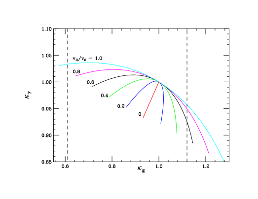
Before discussing our global fit to the 5 parameters present in this simplified model, it is useful to understand the effect mixing has on the SM-like Higgs properties and what can be learned in the future from more precise measurements. Clearly, as we saw above, since κW,Z,b,τ=cθ1subscript𝜅𝑊𝑍𝑏𝜏subscript𝑐𝜃1\kappa_{W,Z,b,\tau}=c_{\theta}\leq 1, determinations of these quantities in excess of unity are outside of the parameter space allowed by our simplified model. If any such values were obtained the model would be excluded. For the loop-induced couplings κg,γsubscript𝜅𝑔𝛾\kappa_{g,\gamma} the situation is less straightforward since both of these quantities depend upon the parameters sθsubscript𝑠𝜃s_{\theta} and rvH/vS𝑟subscript𝑣𝐻subscript𝑣𝑆r\equiv v_{H}/v_{S} in different, yet correlated, ways. In the left panel of Fig. 1, we show the region in the κgκγsubscript𝜅𝑔subscript𝜅𝛾\kappa_{g}-\kappa_{\gamma} plane that is accessible in our simplified model assuming that |sθ|0.35subscript𝑠𝜃0.35|s_{\theta}|\leq 0.35, roughly the range allowed by our global fit to be discussed below. Each curve corresponds to a fixed value of 0r10𝑟10\leq r\leq 1 while the value of sθsubscript𝑠𝜃s_{\theta} is allowed to vary along each of the curves; it is clear that the full allowed region is contained to an ellipse in this plane. Here we see that values of κg>1subscript𝜅𝑔1\kappa_{g}>1 are associated with values of κγ<1subscript𝜅𝛾1\kappa_{\gamma}<1, and vice versa, and that both parameters cannot simultaneously exceed unity. We also observe that values of κγ1.04greater-than-or-equivalent-tosubscript𝜅𝛾1.04\kappa_{\gamma}\gtrsim 1.04 are not allowed in this simplified model. Again, a measurement of either or both of these two quantities outside the locus of points shown here would exclude this model.
Refer to caption Refer to caption

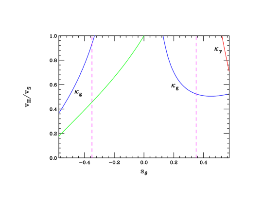
Figure 1: (Left) The region of the κgsubscript𝜅𝑔\kappa_{g}-κγsubscript𝜅𝛾\kappa_{\gamma} plane that is allowed in the simplified model discussed in the text. From outside going inwards (cyan to red) the curves correspond to values of rvH/vS𝑟subscript𝑣𝐻subscript𝑣𝑆r\equiv v_{H}/v_{S} ranging from 1 to zero in steps of 0.2. The value of sθsubscript𝑠𝜃s_{\theta} varies along each curve over the range -0.35 to 0.35, roughly the range allowed by our fit below, with sθ=0subscript𝑠𝜃0s_{\theta}=0 being located at κg=κγ=1subscript𝜅𝑔subscript𝜅𝛾1\kappa_{g}=\kappa_{\gamma}=1. The vertical dashed lines represent the 95%percent9595\% CL bounds from the combined ATLAS/CMS Higgs coupling analysis. (Right) Constraints in the sθvH/vSsubscript𝑠𝜃subscript𝑣𝐻subscript𝑣𝑆s_{\theta}-v_{H}/v_{S} parameter plane from determinations of κgsubscript𝜅𝑔\kappa_{g} (blue) and κγsubscript𝜅𝛾\kappa_{\gamma} (red) from the ATLAS/CMS Higgs coupling analysis. The allowed region lies below the curves. The values of sθ=±0.35subscript𝑠𝜃plus-or-minus0.35s_{\theta}=\pm 0.35, their approximate limit from our fit below, are also shown as the dashed lines. As discussed in the text, the region above the green curve is where |gh2Tt/gh1Tt|>1subscript𝑔subscript2𝑇𝑡subscript𝑔subscript1𝑇𝑡1|g_{h_{2}Tt}/g_{h_{1}Tt}|>1.

The right hand panel of Fig. 1 shows the impact of the ATLAS/CMS determinations [36] of κg,γsubscript𝜅𝑔𝛾\kappa_{g,\gamma} in the sθvH/vSsubscript𝑠𝜃subscript𝑣𝐻subscript𝑣𝑆s_{\theta}-v_{H}/v_{S} parameter plane. The allowed region from the κg,(γ)subscript𝜅𝑔𝛾\kappa_{g,(\gamma)} constraint lies below the blue (red) curve while the vertical dashed lines show the approximate range of |sθ|0.35subscript𝑠𝜃0.35|s_{\theta}|\leq 0.35 allowed by our global fit described below. Of particular interest, for discussion later below, is the region above the green curve where we find that the ratio of the h2Ttsubscript2𝑇𝑡h_{2}Tt and h1Ttsubscript1𝑇𝑡h_{1}Tt couplings satisfies

gh2Tt2gh1Tt2=(sθrcθcθ+rsθ)2>1,superscriptsubscript𝑔subscript2𝑇𝑡2superscriptsubscript𝑔subscript1𝑇𝑡2superscriptsubscript𝑠𝜃𝑟subscript𝑐𝜃subscript𝑐𝜃𝑟subscript𝑠𝜃21{{g_{h_{2}Tt}^{2}}\over{g_{h_{1}Tt}^{2}}}=\Big{(}{{s_{\theta}-rc_{\theta}}\over{c_{\theta}+rs_{\theta}}}\Big{)}^{2}>1\,, (19)

so that the decay rate for Th2t𝑇subscript2𝑡T\rightarrow h_{2}t can naively be potentially comparable to that for Th1t𝑇subscript1𝑡T\rightarrow h_{1}t.

We now perform a global fit of this simplified model to the Higgs and electroweak precision data. We use the HiggsBounds4.2.0 and HiggsSignals1.4.0 programs [37, 38, 39] and the MultiNest algorithm [40] to fit the ATLAS and CMS Higgs data presented in Table 10 of [36] to our model. As the HiggsBounds program returns whether a parameter point is “allowed” or “not allowed”, we take χallowed2=0subscriptsuperscript𝜒2allowed0\chi^{2}_{\rm{allowed}}=0 and χnotallowed2=104subscriptsuperscript𝜒2notallowedsuperscript104\chi^{2}_{\rm{not\,\,allowed}}=10^{4}. We set the MultiNest parameters to nlive=20,000subscript𝑛𝑙𝑖𝑣𝑒20000n_{live}=20,000 and tol=103𝑡𝑜𝑙superscript103tol=10^{-3} in order to adequately explore the likelihood and parameter space of the model. We also include the Peskin-Takeuchi electroweak precision parameters [41], denoted by S,T𝑆𝑇S,T, in the fit, along with the effects of the correlation matrix [11, 42]. To be specific, we employ the new Higgs singlet contributions to both S𝑆S and T𝑇T as well as those from the isosinglet quark contributions to T𝑇T as given in the first of these references. The isosinglet quark contributions are taken from the second reference with a correction made to their Eq.(90) where 2y1y222y1y22subscript𝑦1subscript𝑦222subscript𝑦1subscript𝑦22y_{1}y_{2}\rightarrow 22y_{1}y_{2}. Our fit makes use of the values and correlations as presented by Cuichini [43]. Note that our fit does not include the effects of direct searches for the T𝑇T-quark from the LHC so that we may make probabilistic statements about the novel Th2t𝑇subscript2𝑡T\rightarrow h_{2}t decays which appear in our model, and their effects on standard LHC limits. We focus in detail on the T𝑇T-quark phenomenology below in Section 5.

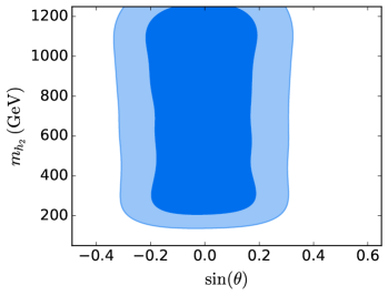
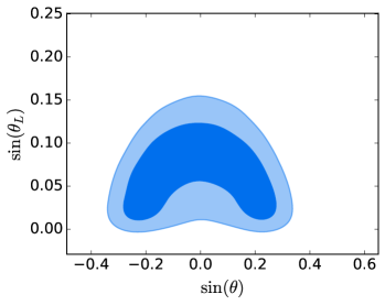
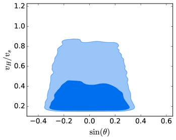
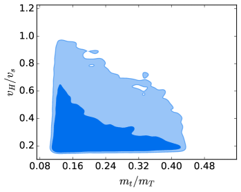
The results of the fit are shown in Fig. 2 and Tab. 2, which also shows the ranges of the parameters we scan over as well as the best-fit values for the parameters. Although we scan over the parameters in Tab. 2, we present our results in terms of sinθ𝜃\sin\theta, sinθLsubscript𝜃𝐿\sin\theta_{L}, mt/mTsubscript𝑚𝑡subscript𝑚𝑇m_{t}/m_{T} and vH/vSsubscript𝑣𝐻subscript𝑣𝑆v_{H}/v_{S} since these are the quantities which enter the physical expressions discussed above. We see that the distribution in mh2subscript𝑚subscript2m_{h_{2}} is relatively flat for mh2subscript𝑚subscript2m_{h_{2}} above 200similar-toabsent200\sim 200 GeV, since once sinθ𝜃\sin\theta is small the h2subscript2h_{2} production cross-sections are suppressed, evading the LHC searches and limits. In turn, sinθ𝜃\sin\theta is forced to be close to 0 (i.e., towards the SM limit) due to the good agreement between the experimentally measured Higgs properties and those predicted in the SM. The sinθ𝜃\sin\theta distribution is slightly asymmetric, and the best-fit point has sinθ<0𝜃0\sin\theta<0, with an overall very slight preference for sinθ<0𝜃0\sin\theta<0 compared to sinθ>0𝜃0\sin\theta>0. Both the ratios vH/vSsubscript𝑣𝐻subscript𝑣𝑆v_{H}/v_{S} and mt/mTsubscript𝑚𝑡subscript𝑚𝑇m_{t}/m_{T} are already driven towards the decoupling limit by current measurements of the Higgs properties (as well as the S𝑆S and T𝑇T parameters), with 68% confidence intervals restricting vH/vS0.85subscript𝑣𝐻subscript𝑣𝑆0.85v_{H}/v_{S}\leq 0.85 and mt/mT0.42subscript𝑚𝑡subscript𝑚𝑇0.42m_{t}/m_{T}\leq 0.42.

Refer to caption Refer to caption

Refer to caption Refer to caption

Figure 2: 68 and 95% Bayesian confidence limit contours (light and dark blue respectively) obtained from the fit to Higgs and precision electroweak data in the (clockwise from top-left) sinθ𝜃\sin\theta-mh2subscript𝑚2m_{h2} , sinθ𝜃\sin\theta-sinθLsubscript𝜃𝐿\sin\theta_{L}, sinθ𝜃\sin\theta-vH/vSsubscript𝑣𝐻subscript𝑣𝑆v_{H}/v_{S} and mt/mTsubscript𝑚𝑡subscript𝑚𝑇m_{t}/m_{T}-vH/vSsubscript𝑣𝐻subscript𝑣𝑆v_{H}/v_{S} parameter planes.
Parameter Range Best fit value
θ𝜃\theta (π/2,π/2)𝜋2𝜋2\left(-\pi/2,\pi/2\right) -0.16
vSsubscript𝑣𝑆v_{S} (GeV) (250.0,1500.0)250.01500.0\left(250.0,1500.0\right) 250 GeV
mTsubscript𝑚𝑇m_{T} (GeV) (250.0,1500.0)250.01500.0\left(250.0,1500.0\right) 400 GeV
θLsubscript𝜃𝐿\theta_{L} (0,π/2)0𝜋2\left(0,\pi/2\right) 0.110.110.11
mh2subscript𝑚2m_{h2} (GeV) (150.0,1250.0)150.01250.0\left(150.0,1250.0\right) 1230 GeV
Table 2: The parameter scan ranges used in the fit to the Higgs data as described in the text, and the best fit values obtained from the fit.

4 Collider Phenomenology of the Scalar Sector

In this section, we examine the phenomenology of the h1,2subscript12h_{1,2} scalar bosons at the LHC. We first explore effects of hh-S𝑆S mixing on h1subscript1h_{1} production rates to determine the degree of difference from Standard Model expectations and then study h2subscript2h_{2} production and decay.

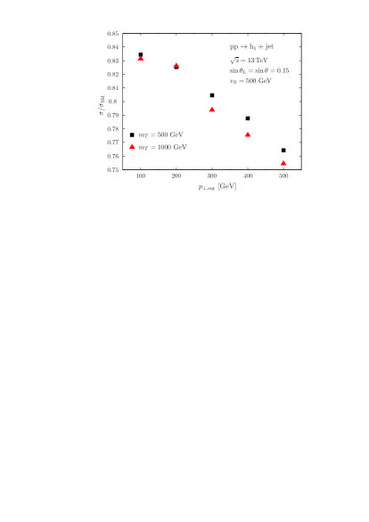
Let us first consider the Higgs plus jet cross section, pph1+jet𝑝𝑝subscript1jetpp\rightarrow h_{1}+{\rm jet}, as a function of a cut on the psubscript𝑝perpendicular-top_{\perp} of the Higgs, Fig. 3 (left). The calculation has been performed with MadGraph5aMC@NLO [44, 45], with the default settings for the parton distribution functions and scales. We have set sinθL=sinθ=0.15subscript𝜃𝐿𝜃0.15\sin\theta_{L}=\sin\theta=0.15 (which is at the outer envelope of the allowed parameter space from the fit, and thus provides an upper bound on how large deviations from the SM can be), and consider two choices for the mass of the vector-like T𝑇T quark, mT=500subscript𝑚𝑇500m_{T}=500 GeV and mT=1subscript𝑚𝑇1m_{T}=1 TeV, respectively. The lower of these masses for mTsubscript𝑚𝑇m_{T} is naively ruled out by current LHC searches, however in models such as ours with allow for dilution of the standard T𝑇T branching ratio the limits may be lower. In the case our choice of mT=500subscript𝑚𝑇500m_{T}=500 GeV, similar to the choices for sinθ𝜃\sin\theta and sinθLsubscript𝜃𝐿\sin\theta_{L} allows us to estimate the maximum size of the deviations away from SM behaviour.

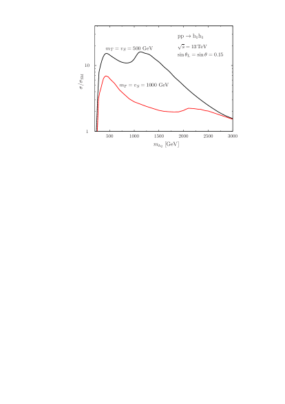
While the emission of a hard jet allows for the exploration of the structure of the heavy fermion loop in principle, see e.g.[46, 47, 48, 49, 50], we see that the deviations from the SM prediction, which ranges from 1.631.631.63 pb for p>100subscript𝑝perpendicular-to100p_{\perp}>100 GeV to 4.54.54.5 fb at p>500subscript𝑝perpendicular-to500p_{\perp}>500 GeV, turn out to be numerically small in our model, given the allowed range of masses and mixings. It will thus be challenging to constrain the properties of the vector-like T𝑇T quark from a measurement of the Higgs+jet cross section. Another way to probe new physics in the Higgs coupling to gluons is through double Higgs production [35, 51, 52, 53]. We show the corresponding cross section, pph1h1𝑝𝑝subscript1subscript1pp\rightarrow h_{1}h_{1} in Fig. 3 (right). Here, we have again set sinθL=sinθ=0.15subscript𝜃𝐿𝜃0.15\sin\theta_{L}=\sin\theta=0.15, and explore the cross section as a function of the mass of the vector-like T𝑇T quark, mTsubscript𝑚𝑇m_{T}, the singlet vacuum expectation value, vSsubscript𝑣𝑆v_{S}, and the mass of the heavy scalar, mh2subscript𝑚subscript2m_{h_{2}}. We find potentially sizable deviations from the SM cross section, σSM=14.6subscript𝜎SM14.6\sigma_{\rm SM}=14.6 fb, resulting from the resonant production pph2h1h1𝑝𝑝subscript2subscript1subscript1pp\rightarrow h_{2}\rightarrow h_{1}h_{1}. The size of the cross section depends not only on the mass of the heavy scalar, but also on the vacuum expectation value vSsubscript𝑣𝑆v_{S} and the mass of the vector-like quark, which leads to a second threshold at mh22mTsimilar-tosubscript𝑚subscript22subscript𝑚𝑇m_{h_{2}}\sim 2m_{T}. The observation of double Higgs production would thus be important to probe new physics in the loop-level coupling of the Higgs to gluons. We further note that previous work has focussed on the cases where there is either a top partner, or a new dihiggs resonance, but in general not both simultaneously.
Refer to caption Refer to caption

Figure 3: (Left) The 125 GeV Higgs plus jet cross section, pph1+jet𝑝𝑝subscript1jetpp\rightarrow h_{1}+{\rm jet}, as a function of a cut on the psubscript𝑝perpendicular-top_{\perp} of the Higgs for s=13𝑠13\sqrt{s}=13 TeV. Shown is the ratio of the simplified Higgs model and the SM prediction, both at leading order, for different values of mTsubscript𝑚𝑇m_{T}. (Right) Higgs pair production, pph1h1𝑝𝑝subscript1subscript1pp\rightarrow h_{1}h_{1}, at 13 TeV, relative to the SM prediction, for two different values of mTsubscript𝑚𝑇m_{T} and vSsubscript𝑣𝑆v_{S}. In both panels we have set sinθL=sinθ=0.15subscript𝜃𝐿𝜃0.15\sin\theta_{L}=\sin\theta=0.15.

We now examine the production and decay of the heavy scalar h2subscript2h_{2} in more detail. Perturbative unitarity considerations can be used to constrain the mass of h2subscript2h_{2} as a function of the input parameters rvH/vS𝑟subscript𝑣𝐻subscript𝑣𝑆r\equiv v_{H}/v_{S} and the hS𝑆h-S mixing angle sθsubscript𝑠𝜃s_{\theta}, once the mass of h1hsimilar-to-or-equalssubscript1h_{1}\simeq h, 125similar-toabsent125\sim 125 GeV is known. To see this, we begin by considering Eq.(47) in Ref. [11] for the h2subscript2h_{2} self-scattering amplitude, h2h2h2h2subscript2subscript2subscript2subscript2h_{2}h_{2}\rightarrow h_{2}h_{2}, which we can write as

=164vH2F(r,sθ,mh2),164superscriptsubscript𝑣𝐻2𝐹𝑟subscript𝑠𝜃subscript𝑚subscript2{\cal M}={1\over{64v_{H}^{2}}}~{}F(r,s_{\theta},m_{h_{2}})\,, (20)

where we define F(r,sθ,mh2)=a(r,sθ)mh22+b(r,sθ)mh12𝐹𝑟subscript𝑠𝜃subscript𝑚subscript2𝑎𝑟subscript𝑠𝜃superscriptsubscript𝑚subscript22𝑏𝑟subscript𝑠𝜃superscriptsubscript𝑚subscript12F(r,s_{\theta},m_{h_{2}})=a(r,s_{\theta})m_{h_{2}}^{2}+b(r,s_{\theta})m_{h_{1}}^{2} with

a(r,sθ)𝑎𝑟subscript𝑠𝜃\displaystyle a(r,s_{\theta}) =\displaystyle= 30(1+r)45(1r)c2+18(1+r)c43(1r)c6+24s23r,301𝑟451𝑟subscript𝑐2181𝑟subscript𝑐431𝑟subscript𝑐624superscriptsubscript𝑠23𝑟\displaystyle 30(1+r)-45(1-r)c_{2}+18(1+r)c_{4}-3(1-r)c_{6}+24s_{2}^{3}\sqrt{r}\,, (21)
b(r,sθ)𝑏𝑟subscript𝑠𝜃\displaystyle b(r,s_{\theta}) =\displaystyle= 6(1+r)3(1r)c26(1+r)c4+3(15)c624s23r.61𝑟31𝑟subscript𝑐261𝑟subscript𝑐4315subscript𝑐624superscriptsubscript𝑠23𝑟\displaystyle 6(1+r)-3(1-r)c_{2}-6(1+r)c_{4}+3(1-5)c_{6}-24s_{2}^{3}\sqrt{r}\,.

Here we have employed the notation cn=cosnθsubscript𝑐𝑛𝑛𝜃c_{n}=\cos n\theta. Since perturbative unitarity requires that ||<1/212|{\cal M}|<1/2, we can easily derive a bound on mh2subscript𝑚subscript2m_{h_{2}} as a function of the input parameters. By using the relation 2GF=1/vH22subscript𝐺𝐹1superscriptsubscript𝑣𝐻2\sqrt{2}G_{F}=1/v_{H}^{2} and defining d=512π/2GF(9.8749TeV)2𝑑512𝜋2subscript𝐺𝐹similar-to-or-equalssuperscript9.8749TeV2d=512\pi/\sqrt{2}G_{F}\simeq(9.8749~{}\rm TeV)^{2} we obtain:

mh2<mh2max=(dbmh12)/a.subscript𝑚subscript2superscriptsubscript𝑚subscript2max𝑑𝑏superscriptsubscript𝑚subscript12𝑎m_{h_{2}}<m_{h_{2}}^{\rm max}={{(d-bm_{h_{1}}^{2})}/{a}}\,. (22)

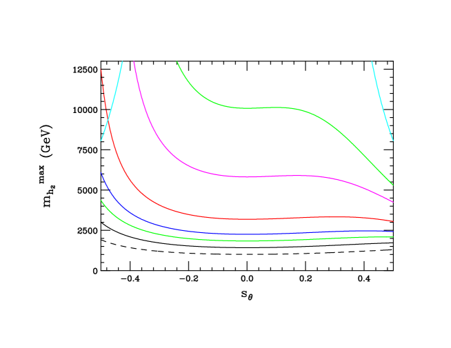
Numerical results using this expression are shown in Fig. 4, where we see several interesting effects: (i𝑖i) For small values of r𝑟r the constraints are rather weak, particularly if |sθ|subscript𝑠𝜃|s_{\theta}| also takes on small values. However as r𝑟r increases the value of mh2maxsuperscriptsubscript𝑚subscript2maxm_{h_{2}}^{\rm max} lies within a range that may be accessible via direct production at the LHC, although probing more of the parameter space would require a higher energy hadron collider. (ii𝑖𝑖ii) Due to the last terms in the expressions for a𝑎a and b𝑏b which are proportional to s23similar-toabsentsuperscriptsubscript𝑠23\sim s_{2}^{3}, the bound is a not an even function of sθsubscript𝑠𝜃s_{\theta} and displays a rather complex hS𝑆h-S mixing angle dependence if r𝑟r is not too large. Likewise the mixing angle dependence of the constraints flattens out when r𝑟r reaches values 0.20.3similar-toabsent0.20.3\sim 0.2-0.3 or greater. (iii𝑖𝑖𝑖iii) When sθ0subscript𝑠𝜃0s_{\theta}\rightarrow 0 the bound simplifies greatly, as in this limit a96r𝑎96𝑟a\rightarrow 96r and b0𝑏0b\rightarrow 0 such that we obtain mh2max1.01TeV/rsimilar-to-or-equalssuperscriptsubscript𝑚subscript2max1.01TeV𝑟m_{h_{2}}^{\rm max}\simeq 1.01~{}{\rm TeV}/\sqrt{r}.

Refer to caption

Figure 4: Constraints on the maximum value of the h2subscript2h_{2} scalar mass from perturbative unitarity of the h2subscript2h_{2} self-scattering amplitude as a function of the hS𝑆h-S mixing sinθ𝜃\sin\theta. From top to bottom (on the right-hand side of the plot) the curves correspond to values of rvH/vS𝑟subscript𝑣𝐻subscript𝑣𝑆r\equiv v_{H}/v_{S} of 0.0, 0.01, 0.03, 0.1, 0.2, 0.3, 0.5 and 1.0. The allowed region of parameter space is below the relevant constraint line.

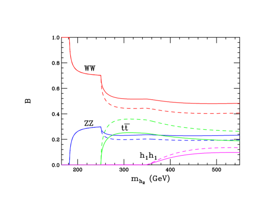
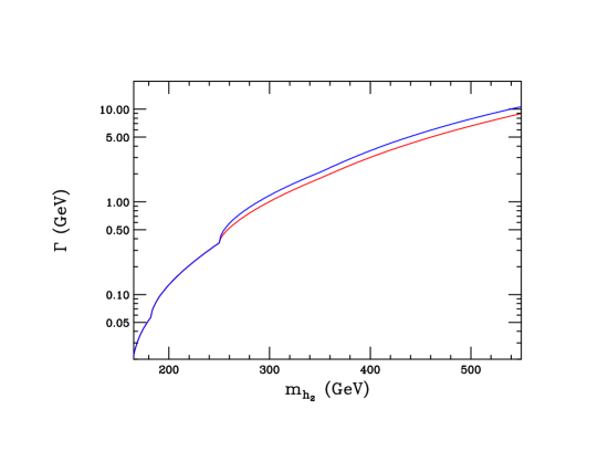
For completeness one might wonder if the sign of sθsubscript𝑠𝜃s_{\theta} also has an important influence on the decays of h2subscript2h_{2} itself. Fig. 5 shows the corresponding h2subscript2h_{2} decay branching fractions for two (different) model points which are identical except for flipping the sign of sθsubscript𝑠𝜃s_{\theta}. The most obvious difference due to the sign in this example is the partial suppression of the gauge modes in favor of the light Higgs and top-quark final states when the sign of sθsubscript𝑠𝜃s_{\theta} is flipped, although the effects are relatively mild. We also see from the right-hand panel of this figure that the h2subscript2h_{2} total width is not much influenced by this choice of sign for these fixed values of the other model parameters.
Refer to caption Refer to caption

Figure 5: (Left) Branching fractions for h2subscript2h_{2} as a function of its mass for W+Wsuperscript𝑊superscript𝑊W^{+}W^{-}(red), ZZ𝑍𝑍ZZ(blue), tt¯𝑡¯𝑡t\bar{t}(green) and h1h1subscript1subscript1h_{1}h_{1}(magenta) final states, assuming that decays into the T𝑇T-quark are kinematically inaccessible. Decays to bb¯𝑏¯𝑏b\bar{b} and lighter states have been neglected. Here we assume vS=500subscript𝑣𝑆500v_{S}=500 GeV, sL=0.15subscript𝑠𝐿0.15s_{L}=0.15 and sθ=0.15(0.15)subscript𝑠𝜃0.150.15s_{\theta}=-0.15(0.15), corresponding to the dashed(solid) curves. (Right) The total h2subscript2h_{2} decay width as a function of its mass in these two scenarios with the blue(red) curve corresponding to the case of sθ>0(sθ<0)subscript𝑠𝜃0subscript𝑠𝜃0s_{\theta}>0(s_{\theta}<0).

Refer to caption Refer to caption

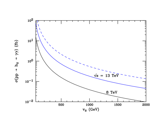
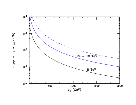
Figure 6: (Left) The cross-sections at 8 and 13 TeV for resonant pph2γγ𝑝𝑝subscript2𝛾𝛾pp\rightarrow h_{2}\rightarrow\gamma\gamma production as a function of the singlet vev vssubscript𝑣𝑠v_{s}. (Right) The cross-sections at 8 and 13 TeV for resonant pph2jj𝑝𝑝subscript2𝑗𝑗pp\rightarrow h_{2}\rightarrow jj production as a function of the singlet vev vssubscript𝑣𝑠v_{s}. Here, mixing has been neglected as discussed in the text and mT=1TeVsubscript𝑚𝑇1𝑇𝑒𝑉m_{T}=1TeV is assumed. The solide blue (black) curve represents s=13,8𝑠138\sqrt{s}=13,8 TeV, while the dashed blue curve corresponds to the case with 3 generations of T𝑇T-quarks contributing to the production at s=13𝑠13\sqrt{s}=13 TeV.

Finally, we discuss the possibility of this simplified model as an explanation for the possible excess of diphoton events at 750 GeV recently reported by the ATLAS and CMS Collaborations in their initial s=13𝑠13\sqrt{s}=13 TeV data set [19, 20]. In order to reproduce this observation, a diphoton resonance with a cross-section of a few inverse femtobarns is required [22, 54]. This cross-section assumes a narrow resonance, and includes the constraints from the 8 TeV diphoton searches. While the ATLAS data suggests a relatively large width of Γ=4050Γ4050\Gamma=40-50 GeV, the CMS results are consistent with the new state being narrow, yet consistent with a wide resonance at the 2σ2𝜎2\sigma level. The work of [54] shows that a global fit to the 8 and 13 TeV data slightly prefers a narrow resonance.

A number of theoretical studies have suggested that this could be explained by the presence of a singlet scalar resonance and heavy vector-like fermions [21, 22, 23, 24, 25, 26, 27, 28, 29, 55]. Such a resonance is required to be mostly-singlet in order to suppress tree-level decays to massive SM fermions and vector bosons. We show in the left panel of Fig. 6 the cross-sections for pph2γγ𝑝𝑝subscript2𝛾𝛾pp\rightarrow h_{2}\rightarrow\gamma\gamma at 8 and 13 TeV for mT=1subscript𝑚𝑇1m_{T}=1 TeV assuming no mixing, i.e., sθ0similar-tosubscript𝑠𝜃0s_{\theta}\sim 0 and sL0similar-tosubscript𝑠𝐿0s_{L}\sim 0. The solid blue (black) curves correspond to s=13(8)𝑠138\sqrt{s}=13(8) TeV. The K-factor is set to be 2.0 according to [56, 57, 58]. We set the hS𝑆h-S mixing to zero for simplicity, as it will not have much influence on the production rate and this easily prevents h2subscript2h_{2} decays into the electroweak gauge bosons W𝑊W and Z𝑍Z. The quark mixing is set to vanish in order to avoid tt¯𝑡¯𝑡t\bar{t} decays of the h2subscript2h_{2} which are not observed, and thus increases its diphoton branching fraction. Fitting the observed cross-section requires vssubscript𝑣𝑠v_{s} to take on values of the order of 100 GeV. This borders on exceeding the perturbative unitarity constraints discussed earlier, a fact which has already been noted in the literature by some. The blue dashed curve in this figures represents the case where there are 3 degenerate generations of T𝑇T-quarks, which all contribution at loop-level to h2subscript2h_{2} production and decay. We see that in this case, perturbative values of the vev vSsubscript𝑣𝑆v_{S} allow for a production rate that is consistent with observations.

The production of the h2subscript2h_{2} resonance in gluon fusion also implies that there must be a corresponding dijet signal. In the right-hand panel of Fig. 6 we show the pph2jj𝑝𝑝subscript2𝑗𝑗pp\rightarrow h_{2}\rightarrow jj cross-section at 8 and 13 TeV. It is clear that current LHC dijet analyses do not yet constrain this parameter space, although this may change in the near future through trigger-level analyses. We note that the h2subscript2h_{2} resonance is narrow with a width always less than a GeV.

5 T𝑇T Production and Decay at the LHC

In this section we explore the phenomenology of the heavy vector-like T𝑇T-quark. Before turning our attention to its production rate and decay modes, we first examine the constraints derived from perturbative unitarity considerations of the T𝑇T self-scattering amplitude.

In a manner similar to the case of h2subscript2h_{2} discussed above, the mass of the T𝑇T-quark can also be constrained as a function of rvH/vS𝑟subscript𝑣𝐻subscript𝑣𝑆r\equiv v_{H}/v_{S} and sLsubscript𝑠𝐿s_{L} by employing perturbative unitarity requirements. To see this, we employ Eqs.(49)-(51) for the TT¯𝑇¯𝑇T\overline{T} scattering amplitude in Ref. [11] and require ||<8π8𝜋|{\cal M}|<8\pi. From this we obtain the constraint

mT<mTmax=[8π2GF]1/2[r(1sL2)2+sL4]1/2.subscript𝑚𝑇superscriptsubscript𝑚𝑇maxsuperscriptdelimited-[]8𝜋2subscript𝐺𝐹12superscriptdelimited-[]𝑟superscript1superscriptsubscript𝑠𝐿22superscriptsubscript𝑠𝐿412m_{T}<m_{T}^{\rm max}=\Bigg{[}{{8\pi}\over{\sqrt{2}G_{F}}}\Bigg{]}^{1/2}\Big{[}r(1-s_{L}^{2})^{2}+s_{L}^{4}\Big{]}^{-1/2}\,. (23)

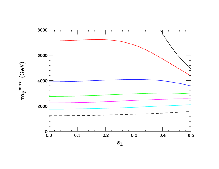
This bound is explored numerically in Fig. 7, where we note several points: (i𝑖i) mTmaxsuperscriptsubscript𝑚𝑇maxm_{T}^{\rm max} is an even function of sLsubscript𝑠𝐿s_{L} and is relatively independent of sLsubscript𝑠𝐿s_{L} in the range of interest once r<0.3𝑟0.3r<0.3. (ii𝑖𝑖ii) If r>0.2𝑟0.2r>0.2, mTmaxsuperscriptsubscript𝑚𝑇maxm_{T}^{\rm max} lies within the range accessible to the LHC. (iii𝑖𝑖𝑖iii) Furthermore, once sLsubscript𝑠𝐿s_{L} is relatively small the bound simplifies to mTmax1.23TeV/rsimilar-to-or-equalssuperscriptsubscript𝑚𝑇max1.23TeV𝑟m_{T}^{\rm max}\simeq 1.23~{}{\rm TeV}/\sqrt{r}. These unitarity bounds demonstrate that a 100 TeV collider is likely required to fully probe the properties and existence of the top partner.
Refer to caption

Figure 7: Constraints on the maximum value of the T𝑇T-quark mass from perturbative unitarity of the T𝑇T self-scattering amplitude. From top to bottom (on the right-hand side of the plot) the curves correspond to values of rvH/vS𝑟subscript𝑣𝐻subscript𝑣𝑆r\equiv v_{H}/v_{S} of 0.0, 0.03, 0.1, 0.2, 0.3, 0.5 and 1.0. The allowed region of parameter space is below the relevant constraint line.

Refer to caption       Refer to caption

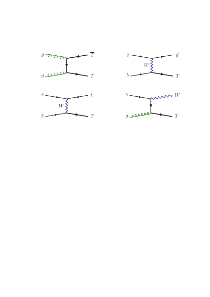
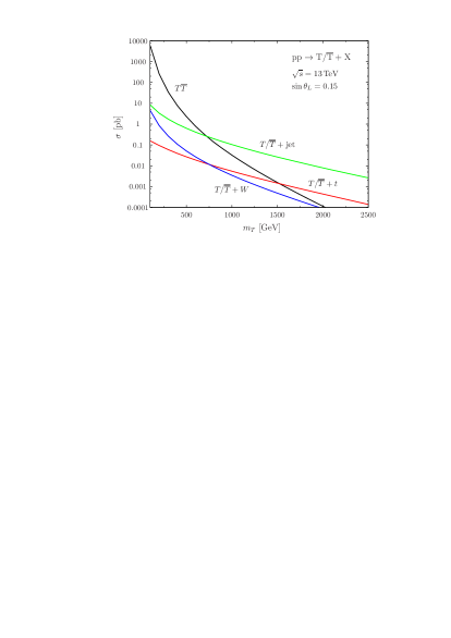
Figure 8: (Left) Exemplary Feynman diagrams for TT¯𝑇¯𝑇T\overline{T} (top-left) and single T𝑇T production at the LHC. (Right) The gg,qq¯TT¯𝑔𝑔𝑞¯𝑞𝑇¯𝑇gg,q\bar{q}\rightarrow T\overline{T} production cross section at 13 TeV (black) and the corresponding single T𝑇T production by several mechanisms: qbqT𝑞𝑏superscript𝑞𝑇qb\rightarrow q^{\prime}T (i.e., T+limit-from𝑇T+jet in green), gbWT𝑔𝑏𝑊𝑇gb\rightarrow WT (i.e., T+W𝑇𝑊T+W in blue) and qq¯,bb¯Tt𝑞¯𝑞𝑏¯𝑏𝑇𝑡q\bar{q},b\bar{b}\rightarrow Tt (i.e., T+t𝑇𝑡T+t in red). We have taken sL=0.15subscript𝑠𝐿0.15s_{L}=0.15.

5.1 Production

As is the case for any new color-triplet fermion, TT¯𝑇¯𝑇T\overline{T} production proceeds at leading order in QCD via both qq¯𝑞¯𝑞q\bar{q} and gg𝑔𝑔gg annihilation, analogous to tt¯𝑡¯𝑡t\bar{t} production in the SM. We show an example Feynman diagramn for the ggTT¯𝑔𝑔𝑇¯𝑇gg\rightarrow T\overline{T} process in Fig. 8 left in the upper-left hand corner. This production rate is quite large even for T𝑇T masses of order 1similar-toabsent1\sim 1 TeV as can be seen in the right-hand panel of Fig. 8 which shows the cross-section at 13 TeV as a function of the T𝑇T-quark mass. Resonant TT¯𝑇¯𝑇T\overline{T} production can also occur through gluon fusion ggh2TT¯𝑔𝑔subscript2𝑇¯𝑇gg\rightarrow h_{2}\rightarrow T\overline{T} when 2mTmh22subscript𝑚𝑇subscript𝑚subscript22m_{T}\leq m_{h_{2}}. Given the current limits on mTsubscript𝑚𝑇m_{T}, this is unlikely to be relevant at the LHC, although it may be observable at a future higher-energy hadron collider.

Due to the potentially significant tT𝑡𝑇t-T mixing within the present scenario, somewhat more interesting single-T𝑇T production processes can also occur; examples of these production mechanisms are depicted in the left-hand panel of Fig. 8. It is clear that single T𝑇T-quark production can occur via several channels, in analogy to single top production in the SM. This can occur in a variety of ways, for example via t𝑡t-channel W𝑊W-exchange, qbqT𝑞𝑏superscript𝑞𝑇qb\rightarrow q^{\prime}T, which corresponds to single top production in the SM except that now the T𝑇T is more massive than the t𝑡t and the coupling, as discussed above, is suppressed by an additional factor of sLsubscript𝑠𝐿s_{L}. Similarly, W+T𝑊𝑇W+T associated production, gbWT𝑔𝑏𝑊𝑇gb\rightarrow WT, can occur via s𝑠s-channel b𝑏b-exchange as well as t𝑡t-channel T𝑇T-exchange which is again analogous to single t𝑡t production in the SM except for the larger T𝑇T mass and the amplitude-level suppression by a factor of sLsubscript𝑠𝐿s_{L}. Taking sL=0.15subscript𝑠𝐿0.15s_{L}=0.15 as a large, but allowed, value of the mixing given our above fit, Fig. 8 shows that these cross sections can be quite significant, particularly for large T𝑇T masses [15, 16]. We find that for mT750greater-than-or-equivalent-tosubscript𝑚𝑇750m_{T}\gtrsim 750 GeV the T+limit-from𝑇T+jet single production rate is larger than that for pair production from QCD due to the significant phase-space suppression. For other values of sLsubscript𝑠𝐿s_{L}, the cross sections for these processes can be easily obtained from the figure by rescaling by a factor of (sL/0.15)2superscriptsubscript𝑠𝐿0.152(s_{L}/0.15)^{2}. Finally, the single T𝑇T production process qq¯,bb¯t¯T+h.c.formulae-sequence𝑞¯𝑞𝑏¯𝑏¯𝑡𝑇𝑐q\bar{q},b\bar{b}\rightarrow\bar{t}T+h.c. can also now occur via t𝑡t-channel W𝑊W-exchange as well as s𝑠s-channel flavor-changing Z𝑍Z-exchange which leads to the smallest rate shown in the figure. Recall that this flavor-changing coupling arises from the fact that tLsubscript𝑡𝐿t_{L} and TLsubscript𝑇𝐿T_{L} have different values of the third component of weak isospin, T3Lsubscript𝑇3𝐿T_{3L}. In this case the cross section scales as (sLcL)2superscriptsubscript𝑠𝐿subscript𝑐𝐿2(s_{L}c_{L})^{2}.

Of course tT¯+h.c.formulae-sequence𝑡¯𝑇𝑐t\overline{T}+h.c. production can also occur from both gg𝑔𝑔gg and qq¯𝑞¯𝑞q\bar{q} initial states via QCD through a loop-induced flavor-changing (tT¯+Tt¯)g𝑡¯𝑇𝑇¯𝑡𝑔(t\overline{T}+T\bar{t})g coupling. Such an interaction vertex will be not only loop-suppressed but will also involve the familiar factors of the tT𝑡𝑇t-T mixing angle, sLsubscript𝑠𝐿s_{L}, leading to an even further suppression, and we do not consider it further in this work.

5.2 Decays

Tt𝑇𝑡T-t mixing allows for the decay of the T𝑇T-quark and without which T𝑇T would be stable. Within the present framework, any discussion of T𝑇T decays (and the collider searches for T𝑇T) necessarily involves the role of the additional mostly-singlet Higgs field, h2subscript2h_{2}. The tree-level decay modes of T𝑇T (if they are kinematically allowed) are TWb,Zt,h1t𝑇𝑊𝑏𝑍𝑡subscript1𝑡T\rightarrow Wb,Zt,h_{1}t and h2tsubscript2𝑡h_{2}t, all of whose corresponding partial widths are proportional to the factor sL2superscriptsubscript𝑠𝐿2s_{L}^{2}. The presence of this ‘exotic’ h2tsubscript2𝑡h_{2}t decay mode, which is absent in almost all discussions of vector-like heavy quark decays, can have a strong potential impact on the searches for T𝑇T-quarks that have been performed so far at the LHC. At present, existing searches only consider the case where the SM is solely augmented by a heavy T𝑇T-quark with no additional h2subscript2h_{2} field being present. Thus these analyses all make the common assumption that the sum of the branching fractions for the Wb,Zt𝑊𝑏𝑍𝑡Wb,Zt and h1tsubscript1𝑡h_{1}t decay modes must sum to unity and lower bounds on the T𝑇T mass have been obtained for different branching fraction weights [59, 60]. Under this assumption, ATLAS and CMS obtain the 95%percent\% CL lower bound of mT715730greater-than-or-equivalent-tosubscript𝑚𝑇715730m_{T}\gtrsim 715-730 GeV with even larger values being obtained as the various T𝑇T-quark branching fractions are scanned over. Since these standard searches rely on reconstructing the T𝑇T mass from the SM decay products, they have minimal sensitivity to the Th2t𝑇subscript2𝑡T\rightarrow h_{2}t decay channel (the exception to this would be if mh1mh2similar-tosubscript𝑚subscript1subscript𝑚subscript2m_{h_{1}}\sim m_{h_{2}} such that the acceptances would be similar). However, as we will see below, there can be a significant region of the model parameter space where the h2tsubscript2𝑡h_{2}t decay mode is kinematically allowed and obtains a respectable coupling strength relative to that for h1tsubscript1𝑡h_{1}t. Clearly the influence of this mode on the lower bound obtained on the T𝑇T mass will depend upon how h2subscript2h_{2} itself decays. We might expect that if the h2subscript2h_{2} decays in a manner broadly similar to the SM-like h1subscript1h_{1} (e.g.  into WW𝑊𝑊WW, ZZ𝑍𝑍ZZ or bb¯𝑏¯𝑏b\bar{b}) the effects will be minimal except that the final state kinematics can be significantly different depending upon both the T𝑇T and h2subscript2h_{2} masses. Of course if h2subscript2h_{2} is sufficiently heavy, the branching ratio for the decay h2tt¯subscript2𝑡¯𝑡h_{2}\rightarrow t\bar{t} can be significant so that the decay path Tttt¯𝑇𝑡𝑡¯𝑡T\rightarrow tt\bar{t} via virtual h2subscript2h_{2} exchange opens up, this has also not been examined in T𝑇T-quark searches. Clearly a detailed analysis of how the existence of a non-negligible branching fraction for T𝑇T into the h2tsubscript2𝑡h_{2}t mode would affect the searches for T𝑇T-quarks at the LHC remains an open question that needs to be performed in detail, but we might expect that if this branching fraction is sufficiently small the ‘standard’ limits discussed above will approximately apply.
Refer to caption Refer to caption

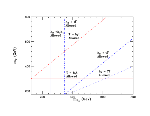
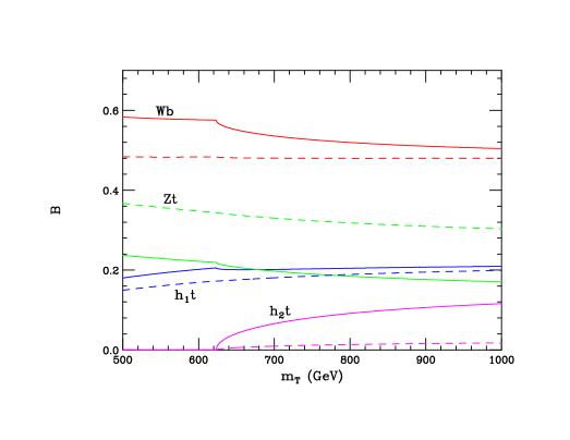
Figure 9: (Left) Kinematic regions for the various decays of h2subscript2h_{2} and T𝑇T in the mh2mTsubscript𝑚subscript2subscript𝑚𝑇m_{h_{2}}-m_{T} plane. To the right of the blue solid (dash-dotted, dashed, dotted) lines the decay h2h1h1(tt¯,tT¯+h.c.,TT¯)h_{2}\rightarrow h_{1}h_{1}(t\bar{t},~{}t\overline{T}+h.c.,T\overline{T}) are kinematically allowed. In the region above the red solid (dash-dotted) line the decay Th1t(h2t)𝑇subscript1𝑡subscript2𝑡T\rightarrow h_{1}t(h_{2}t) is kinematically allowed. (Right) Sample T𝑇T decay branching fractions as a function of mTsubscript𝑚𝑇m_{T} assuming mh2=300subscript𝑚subscript2300m_{h_{2}}=300 GeV, sL=0.15subscript𝑠𝐿0.15s_{L}=0.15, vS=500subscript𝑣𝑆500v_{S}=500 GeV and sθ=0.15(0.15)subscript𝑠𝜃0.150.15s_{\theta}=-0.15(0.15) corresponding to the dashed (solid) curves. The branching fractions for the Wb(Zt,h1t,h2t)𝑊𝑏𝑍𝑡subscript1𝑡subscript2𝑡Wb(Zt,~{}h_{1}t,~{}h_{2}t) modes are shown as the red (blue, green, magenta) curves.

To provide some overall understanding of the interplay between the masses of h2subscript2h_{2} and T𝑇T and the corresponding decay physics, the left-hand panel of Fig. 9 gives a semi-quantitative feel for the regions in this space where the various decay modes may occur. The strengths of the various couplings are determined by the three remaining model parameters sθ,sLsubscript𝑠𝜃subscript𝑠𝐿s_{\theta},s_{L} and the ratio of vev’s r=vH/vS𝑟subscript𝑣𝐻subscript𝑣𝑆r=v_{H}/v_{S} and are given in the Appendix. An important example is provided by the ratio of the Th2t𝑇subscript2𝑡T\rightarrow h_{2}t and Th1t𝑇subscript1𝑡T\rightarrow h_{1}t partial widths, R𝑅R, which apart from phase space factors is given by

R=Γ(Th2t)Γ(Th1t)[sθrcθcθ+rsθ]2,𝑅Γ𝑇subscript2𝑡Γ𝑇subscript1𝑡similar-tosuperscriptdelimited-[]subscript𝑠𝜃𝑟subscript𝑐𝜃subscript𝑐𝜃𝑟subscript𝑠𝜃2R={{\Gamma(T\rightarrow h_{2}t)}\over{\Gamma(T\rightarrow h_{1}t)}}\sim\Bigg{[}{{s_{\theta}-rc_{\theta}}\over{c_{\theta}+rs_{\theta}}}\Bigg{]}^{2}\,, (24)

where sθ=sinθsubscript𝑠𝜃𝜃s_{\theta}=\sin\theta and cθ=cosθsubscript𝑐𝜃𝜃c_{\theta}=\cos\theta. Clearly, the parameter space region with somewhat larger r𝑟r values and with sθ<0subscript𝑠𝜃0s_{\theta}<0 can lead to a significant result for this ratio, thus providing a good example of a situation where the sign of sθsubscript𝑠𝜃s_{\theta} is important. In Fig. 9 above, we see that there is a region where R>1𝑅1R>1 is obtained.

The right-hand panel of Fig. 9 compares the branching fractions for the various T𝑇T-quark decay modes for two parameter choices which differ only in the choice of sign for sθsubscript𝑠𝜃s_{\theta}. There can be some significant differences in these two cases: apart from the obviously much larger value for the branching fraction of the h1tsubscript1𝑡h_{1}t mode when sθ>0subscript𝑠𝜃0s_{\theta}>0 we see that the branching fraction for h2tsubscript2𝑡h_{2}t is larger in the sθ<0subscript𝑠𝜃0s_{\theta}<0 case at the expense of that for h1tsubscript1𝑡h_{1}t at larger values of mTsubscript𝑚𝑇m_{T}. On the other hand, we also see that the branching fractions for the Wb,Zt𝑊𝑏𝑍𝑡Wb,Zt decay modes are relatively unaffected by the change of sign of sθsubscript𝑠𝜃s_{\theta}. In general, since κgcθsθrsimilar-to-or-equalssubscript𝜅𝑔subscript𝑐𝜃subscript𝑠𝜃𝑟\kappa_{g}\simeq c_{\theta}-s_{\theta}r, much of the parameter space where the above ratio of decay widths is large is restricted by LHC data at some level since it simultaneously produces a too large value for κgsubscript𝜅𝑔\kappa_{g}.

Refer to caption
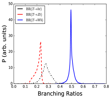
Figure 10: This plot shows the probability distributions of the BR(Th1t)BR𝑇subscript1𝑡\textrm{BR}(T\rightarrow h_{1}t) (black dash-dot), BR(TZt)BR𝑇𝑍𝑡\textrm{BR}(T\rightarrow Zt) (red dotted) and BR(TWb)BR𝑇𝑊𝑏\textrm{BR}(T\rightarrow Wb) (blue solid) branching ratios of the top-partner T𝑇T resulting from our fit to the Higgs and electroweak data. The y𝑦y-axis shows probability in arbitrary units, and the areas of the three branching ratio curves have all been individually normalised to one.

While this discussion describes the phenomenology that is possible, given the results of our fit, we can also ask about the probable decays of T𝑇T. We show in Fig. 10 the probability distributions for the branching ratios of T𝑇T decaying into SM final states: Th1t𝑇subscript1𝑡T\rightarrow h_{1}t, TZt𝑇𝑍𝑡T\rightarrow Zt and TWb𝑇𝑊𝑏T\rightarrow Wb in dot-dash black, dashed red and solid blue, respectively. We find that it is most likely given current data that the central values of the probability distribution for the branching ratios are close to the well-known ratios of 25:25:50:2525:5025:25:50. However, there is substantial room for non-standard branching ratios with all decay channels subjection to variation on the order of 10%. As discussed above, given the wide allowed ranges for the parameters, we also found it possible that the BR(Th2t)BR𝑇subscript2𝑡\mathrm{BR}(T\rightarrow h_{2}t) maybe be as large as 10%.

6 Conclusion

We have formulated a set of simplified models to characterize the interactions of physics beyond the Standard Model with the 125 GeV Higgs boson. We selected one such model, where the Standard Model is extended by a gauge singlet scalar and vector-like fermions which mix with the SM top-quarks, and studied its phenomenology in detail. In particular, we examined the complementarity between indirect searches for new physics in precise determinations of the 125 GeV Higgs couplings and distributions with direct searches for new particles. We constrained the model parameters by performing a global fit using the ATLAS and CMS combined data on the Higgs couplings and searches for heavy new scalars. We argued that although our model allows for the possibility of exotic top partner phenomenology, it is robustly constrained by top partner searches from LHC Run 1. Nonetheless, the top-partner decay into a SM top-quark and new heavy scalar, Tth2𝑇𝑡subscript2T\rightarrow th_{2}, would lead to novel signatures and deserves to be better explored with Run 2 searches in mind. We find that given current direct search constraints, the effects of the top partners in Higgs loops are mostly likely too small to observe, in line with general expectations in weakly coupled models. We also note that our model (at least in the case a single generation of top partners) is unable to explain a possible 750 GeV diphoton resonance which has recently been reported by ATLAS and CMS without resorting to non-perturbative couplings. As the LHC moves further into the precision era, simplified models for Higgs physics will serve as a test-bed for expectations of possible BSM signals in the Higgs sector and direct searches for new particles.

Acknowledgement

We thank Tim Stefaniak for assistance with the ATLAS+CMS combination in HiggsSignals. The research of MD was performed in part at the Munich Institute for Astro- and Particle Physics (MIAPP), part of the DFG cluster of excellence “Origin and Structure of the Universe”. MK would like to thank SLAC and the SLAC Theory group for hospitality and support. The work of MK is supported by the German Research Foundation DFG through the research unit 2239 “New physics at the LHC”. The work of JLH and TGR was supported by the U.S. Department of Energy, Contract DE-AC02-76SF00515.

Appendix A Model details

A.1 The scalar potential

To minimize the potential in Eq.(6), we need to solve

V(h,s)h|H=vH/2,S=vS=V(h,s)s|H=vH/2,S=vS=0.evaluated-at𝑉𝑠formulae-sequencedelimited-⟨⟩𝐻subscript𝑣𝐻2delimited-⟨⟩𝑆subscript𝑣𝑆evaluated-at𝑉𝑠𝑠formulae-sequencedelimited-⟨⟩𝐻subscript𝑣𝐻2delimited-⟨⟩𝑆subscript𝑣𝑆0\left.\frac{\partial V(h,s)}{\partial h}\right|_{\langle H\rangle=v_{H}/\sqrt{2},\langle S\rangle=v_{S}}=\left.\frac{\partial V(h,s)}{\partial s}\right|_{\langle H\rangle=v_{H}/\sqrt{2},\langle S\rangle=v_{S}}=0. (25)

For a minimum, we also need 2V/s2>0superscript2𝑉superscript𝑠20\partial^{2}V/\partial s^{2}>0, 2V/h2>0superscript2𝑉superscript20\partial^{2}V/\partial h^{2}>0, and 2V/s22V/h2(2V/(sh))2>0superscript2𝑉superscript𝑠2superscript2𝑉superscript2superscriptsuperscript2𝑉𝑠20\partial^{2}V/\partial s^{2}\,\partial^{2}V/\partial h^{2}-(\partial^{2}V/(\partial s\partial h))^{2}>0. We find

Vh𝑉\displaystyle\frac{\partial V}{\partial h} =\displaystyle= μ2(h+vH)+λ(h+vH)3superscript𝜇2subscript𝑣𝐻𝜆superscriptsubscript𝑣𝐻3\displaystyle-\mu^{2}(h+v_{H})+\lambda(h+v_{H})^{3} (26)
+a12(h+vH)(s+vS)+a22(h+vH)(s+vS)2,subscript𝑎12subscript𝑣𝐻𝑠subscript𝑣𝑆subscript𝑎22subscript𝑣𝐻superscript𝑠subscript𝑣𝑆2\displaystyle+\frac{a_{1}}{2}(h+v_{H})(s+v_{S})+\frac{a_{2}}{2}(h+v_{H})(s+v_{S})^{2}\,,
2Vh2superscript2𝑉superscript2\displaystyle\frac{\partial^{2}V}{\partial h^{2}} =\displaystyle= μ2+3λ(h+vH)2+a12(s+vS)+a22(s+vS)2,superscript𝜇23𝜆superscriptsubscript𝑣𝐻2subscript𝑎12𝑠subscript𝑣𝑆subscript𝑎22superscript𝑠subscript𝑣𝑆2\displaystyle-\mu^{2}+3\lambda(h+v_{H})^{2}+\frac{a_{1}}{2}(s+v_{S})+\frac{a_{2}}{2}(s+v_{S})^{2}\,, (27)
Vs𝑉𝑠\displaystyle\frac{\partial V}{\partial s} =\displaystyle= a14(h+vH)2+a22(h+vH)2(s+vS)subscript𝑎14superscriptsubscript𝑣𝐻2subscript𝑎22superscriptsubscript𝑣𝐻2𝑠subscript𝑣𝑆\displaystyle\frac{a_{1}}{4}(h+v_{H})^{2}+\frac{a_{2}}{2}(h+v_{H})^{2}(s+v_{S}) (28)
+b1+b2(s+vS)+b3(s+vS)2+b4(s+vS)3,subscript𝑏1subscript𝑏2𝑠subscript𝑣𝑆subscript𝑏3superscript𝑠subscript𝑣𝑆2subscript𝑏4superscript𝑠subscript𝑣𝑆3\displaystyle+b_{1}+b_{2}(s+v_{S})+b_{3}(s+v_{S})^{2}+b_{4}(s+v_{S})^{3}\,,
2Vs2superscript2𝑉superscript𝑠2\displaystyle\frac{\partial^{2}V}{\partial s^{2}} =\displaystyle= a22(h+vH)2+b2+2b3(s+vS)+3b4(s+vS)2,subscript𝑎22superscriptsubscript𝑣𝐻2subscript𝑏22subscript𝑏3𝑠subscript𝑣𝑆3subscript𝑏4superscript𝑠subscript𝑣𝑆2\displaystyle\frac{a_{2}}{2}(h+v_{H})^{2}+b_{2}+2b_{3}(s+v_{S})+3b_{4}(s+v_{S})^{2}\,, (29)
2Vshsuperscript2𝑉𝑠\displaystyle\frac{\partial^{2}V}{\partial s\partial h} =\displaystyle= (h+vH)(a12+a2(s+vS)).subscript𝑣𝐻subscript𝑎12subscript𝑎2𝑠subscript𝑣𝑆\displaystyle(h+v_{H})\,\left(\frac{a_{1}}{2}+a_{2}(s+v_{S})\right). (30)

Thus the conditions for a minimum are (assuming vH,vS>0subscript𝑣𝐻subscript𝑣𝑆0v_{H},v_{S}>0):

μ2+λvH2+a12vS+a22vS2superscript𝜇2𝜆superscriptsubscript𝑣𝐻2subscript𝑎12subscript𝑣𝑆subscript𝑎22superscriptsubscript𝑣𝑆2\displaystyle-\mu^{2}+\lambda v_{H}^{2}+\frac{a_{1}}{2}v_{S}+\frac{a_{2}}{2}v_{S}^{2} =\displaystyle= 0,0\displaystyle 0\,, (31)
a14vH2+a22vH2vS+b1+b2vS+b3vS2+b4vS3subscript𝑎14superscriptsubscript𝑣𝐻2subscript𝑎22superscriptsubscript𝑣𝐻2subscript𝑣𝑆subscript𝑏1subscript𝑏2subscript𝑣𝑆subscript𝑏3superscriptsubscript𝑣𝑆2subscript𝑏4superscriptsubscript𝑣𝑆3\displaystyle\frac{a_{1}}{4}v_{H}^{2}+\frac{a_{2}}{2}v_{H}^{2}v_{S}+b_{1}+b_{2}v_{S}+b_{3}v_{S}^{2}+b_{4}v_{S}^{3} =\displaystyle= 0,0\displaystyle 0\,, (32)
λ𝜆\displaystyle\lambda >\displaystyle> 0,0\displaystyle 0\,, (33)
a22vH2+b2+2b3vS+3b4vS2subscript𝑎22superscriptsubscript𝑣𝐻2subscript𝑏22subscript𝑏3subscript𝑣𝑆3subscript𝑏4superscriptsubscript𝑣𝑆2\displaystyle\frac{a_{2}}{2}v_{H}^{2}+b_{2}+2b_{3}v_{S}+3b_{4}v_{S}^{2} >\displaystyle> 0,0\displaystyle 0\,, (34)
2λvH2(a22vH2+b2+2b3vS+3b4vS2)vH2(a12+a2vS)22𝜆superscriptsubscript𝑣𝐻2subscript𝑎22superscriptsubscript𝑣𝐻2subscript𝑏22subscript𝑏3subscript𝑣𝑆3subscript𝑏4superscriptsubscript𝑣𝑆2superscriptsubscript𝑣𝐻2superscriptsubscript𝑎12subscript𝑎2subscript𝑣𝑆2\displaystyle 2\lambda v_{H}^{2}\left(\frac{a_{2}}{2}v_{H}^{2}+b_{2}+2b_{3}v_{S}+3b_{4}v_{S}^{2}\right)-v_{H}^{2}\left(\frac{a_{1}}{2}+a_{2}v_{S}\right)^{2} >\displaystyle> 0.0\displaystyle 0. (35)

The physical masses of the two scalar particles are determined by the mass matrix

V(h,s)12(hs)(M112M122M122M222)(hs),12𝑠matrixsuperscriptsubscript𝑀112superscriptsubscript𝑀122superscriptsubscript𝑀122superscriptsubscript𝑀222matrix𝑠𝑉𝑠V(h,s)\supset\frac{1}{2}(h\;s)\begin{pmatrix}M_{11}^{2}&M_{12}^{2}\\ M_{12}^{2}&M_{22}^{2}\end{pmatrix}\begin{pmatrix}h\\ s\end{pmatrix}, (36)

where

M112superscriptsubscript𝑀112\displaystyle M_{11}^{2} =\displaystyle= 2Vh2|H=vH/2,S=vS= 2λvH2+a12vS,evaluated-atsuperscript2𝑉superscript2formulae-sequencedelimited-⟨⟩𝐻subscript𝑣𝐻2delimited-⟨⟩𝑆subscript𝑣𝑆2𝜆superscriptsubscript𝑣𝐻2subscript𝑎12subscript𝑣𝑆\displaystyle\left.\frac{\partial^{2}V}{\partial h^{2}}\right|_{\langle H\rangle=v_{H}/\sqrt{2},\langle S\rangle=v_{S}}\;\;\,=\;2\lambda v_{H}^{2}+\frac{a_{1}}{2}v_{S}\,, (37)
M222superscriptsubscript𝑀222\displaystyle M_{22}^{2} =\displaystyle= 2Vs2|H=vH/2,S=vS=a22vH2+b2+2b3vS+3b4vS2,evaluated-atsuperscript2𝑉superscript𝑠2formulae-sequencedelimited-⟨⟩𝐻subscript𝑣𝐻2delimited-⟨⟩𝑆subscript𝑣𝑆subscript𝑎22superscriptsubscript𝑣𝐻2subscript𝑏22subscript𝑏3subscript𝑣𝑆3subscript𝑏4superscriptsubscript𝑣𝑆2\displaystyle\left.\frac{\partial^{2}V}{\partial s^{2}}\right|_{\langle H\rangle=v_{H}/\sqrt{2},\langle S\rangle=v_{S}}\;\;\,=\;\frac{a_{2}}{2}v_{H}^{2}+b_{2}+2b_{3}v_{S}+3b_{4}v_{S}^{2}\,, (38)
M122superscriptsubscript𝑀122\displaystyle M_{12}^{2} =\displaystyle= 2Vsh|H=vH/2,S=vS=(a12+a2vS)vH.evaluated-atsuperscript2𝑉𝑠formulae-sequencedelimited-⟨⟩𝐻subscript𝑣𝐻2delimited-⟨⟩𝑆subscript𝑣𝑆subscript𝑎12subscript𝑎2subscript𝑣𝑆subscript𝑣𝐻\displaystyle\left.\frac{\partial^{2}V}{\partial s\partial h}\right|_{\langle H\rangle=v_{H}/\sqrt{2},\langle S\rangle=v_{S}}\,\,=\;\left(\frac{a_{1}}{2}+a_{2}v_{S}\right)v_{H}. (39)

The physical masses are

m1,22=12(M112+M222(M112M222)2+4M124),superscriptsubscript𝑚12212minus-or-plussuperscriptsubscript𝑀112superscriptsubscript𝑀222superscriptsuperscriptsubscript𝑀112superscriptsubscript𝑀22224superscriptsubscript𝑀124m_{1,2}^{2}=\frac{1}{2}\left(M_{11}^{2}+M_{22}^{2}\mp\sqrt{(M_{11}^{2}-M_{22}^{2})^{2}+4M_{12}^{4}}\right), (40)

where we assume that the lighter mass eigenstate corresponds to the SM-like Higgs boson with m1=125subscript𝑚1125m_{1}=125 GeV. The mass eigenstates h1,h2subscript1subscript2h_{1},h_{2} are related to the fields h,s𝑠h,s through

(h1h2)=(cosθsinθsinθcosθ)(hs),matrixsubscript1subscript2matrix𝜃𝜃𝜃𝜃matrix𝑠\begin{pmatrix}h_{1}\\ h_{2}\end{pmatrix}=\begin{pmatrix}\cos\theta&-\sin\theta\\ \sin\theta&\cos\theta\end{pmatrix}\begin{pmatrix}h\\ s\end{pmatrix}, (41)

with

tan(2θ)=2M122M222M112.2𝜃2superscriptsubscript𝑀122superscriptsubscript𝑀222superscriptsubscript𝑀112\tan(2\theta)=\frac{2M_{12}^{2}}{M_{22}^{2}-M_{11}^{2}}. (42)

In the limit vSvHmuch-greater-thansubscript𝑣𝑆subscript𝑣𝐻v_{S}\gg v_{H}, and setting a1=b1=b3=0subscript𝑎1subscript𝑏1subscript𝑏30a_{1}=b_{1}=b_{3}=0, the expressions for the masses and the mixing angle simplify:

m12superscriptsubscript𝑚12\displaystyle m_{1}^{2} =\displaystyle= 2λvH2(1a224λb4),2𝜆superscriptsubscript𝑣𝐻21superscriptsubscript𝑎224𝜆subscript𝑏4\displaystyle 2\lambda v_{H}^{2}\left(1-\frac{a_{2}^{2}}{4\lambda b_{4}}\right)\,, (43)
m22superscriptsubscript𝑚22\displaystyle m_{2}^{2} =\displaystyle= 2b4vS2(1+a224b42vH2vS2),2subscript𝑏4superscriptsubscript𝑣𝑆21superscriptsubscript𝑎224superscriptsubscript𝑏42superscriptsubscript𝑣𝐻2superscriptsubscript𝑣𝑆2\displaystyle 2b_{4}v_{S}^{2}\left(1+\frac{a_{2}^{2}}{4b_{4}^{2}}\frac{v_{H}^{2}}{v_{S}^{2}}\right)\,, (44)
tan(2θ)2𝜃\displaystyle\tan(2\theta) =\displaystyle= a2b4vHvS.subscript𝑎2subscript𝑏4subscript𝑣𝐻subscript𝑣𝑆\displaystyle\frac{a_{2}}{b_{4}}\frac{v_{H}}{v_{S}}. (45)

A.2 The Yukawa potential

Here we calculate the mass mixing between the top quark and the new top partner field T𝑇T. The mass terms have the form

YukawasubscriptYukawa\displaystyle\mathcal{L}_{\rm Yukawa} superset-of\displaystyle\supset (t¯LintT¯Lint)(tRintTRint)subscriptsuperscript¯𝑡int𝐿subscriptsuperscript¯𝑇int𝐿matrixsubscriptsuperscript𝑡int𝑅subscriptsuperscript𝑇int𝑅\displaystyle(\bar{t}^{\rm int}_{L}\;\overline{T}^{\rm int}_{L})\mathcal{M}\begin{pmatrix}t^{\rm int}_{R}\\ T^{\rm int}_{R}\end{pmatrix} (46)
=\displaystyle= (t¯LintT¯Lint)(ytvH/2λTvH/20yTvS)(tRintTRint).subscriptsuperscript¯𝑡int𝐿subscriptsuperscript¯𝑇int𝐿matrixsubscript𝑦𝑡subscript𝑣𝐻2subscript𝜆𝑇subscript𝑣𝐻20subscript𝑦𝑇subscript𝑣𝑆matrixsubscriptsuperscript𝑡int𝑅subscriptsuperscript𝑇int𝑅\displaystyle(\bar{t}^{\rm int}_{L}\;\overline{T}^{\rm int}_{L})\begin{pmatrix}y_{t}v_{H}/\sqrt{2}&\lambda_{T}v_{H}/\sqrt{2}\\ 0&y_{T}v_{S}\end{pmatrix}\begin{pmatrix}t^{\rm int}_{R}\\ T^{\rm int}_{R}\end{pmatrix}. (47)

The physical mass eigenstates tL/Rsubscript𝑡𝐿𝑅t_{L/R} and TL/Rsubscript𝑇𝐿𝑅T_{L/R}, and the mixing angles θL/Rsubscript𝜃𝐿𝑅\theta_{L/R}, are obtained from bi-unitary transformations,

(tL/RTL/R)=𝒰L/R(tL/RintTL/Rint),matrixsubscript𝑡𝐿𝑅subscript𝑇𝐿𝑅subscript𝒰𝐿𝑅matrixsubscriptsuperscript𝑡int𝐿𝑅subscriptsuperscript𝑇int𝐿𝑅\begin{pmatrix}t_{L/R}\\ T_{L/R}\end{pmatrix}=\mathcal{U}_{L/R}\begin{pmatrix}t^{\rm int}_{L/R}\\ T^{\rm int}_{L/R}\end{pmatrix}, (48)

with

𝒰L/R=(cosθL/RsinθL/RsinθL/RcosθL/R).subscript𝒰𝐿𝑅matrixsubscript𝜃𝐿𝑅subscript𝜃𝐿𝑅subscript𝜃𝐿𝑅subscript𝜃𝐿𝑅\mathcal{U}_{L/R}=\begin{pmatrix}\cos\theta_{L/R}&-\sin\theta_{L/R}\\ \sin\theta_{L/R}&\cos\theta_{L/R}\end{pmatrix}. (49)

The mass matrix \mathcal{M} is diagonalized according to

𝒰L𝒰R=(mt00mT)diagsubscript𝒰𝐿superscriptsubscript𝒰𝑅matrixsubscript𝑚𝑡00subscript𝑚𝑇subscriptdiag\mathcal{U}_{L}\mathcal{M}\mathcal{U}_{R}^{\dagger}=\begin{pmatrix}m_{t}&0\\ 0&m_{T}\end{pmatrix}\equiv\mathcal{M}_{\rm diag} (50)

or equivalently

𝒰L𝒰L=𝒰R𝒰R=diag2.subscript𝒰𝐿superscriptsuperscriptsubscript𝒰𝐿subscript𝒰𝑅superscriptsuperscriptsubscript𝒰𝑅superscriptsubscriptdiag2\mathcal{U}_{L}\mathcal{M}\mathcal{M}^{\dagger}\mathcal{U}_{L}^{\dagger}=\mathcal{U}_{R}\mathcal{M}^{\dagger}\mathcal{M}\mathcal{U}_{R}^{\dagger}=\mathcal{M}_{\rm diag}^{2}. (51)

We use

Tr[]Trdelimited-[]superscript\displaystyle{\rm Tr}\,[\mathcal{M}\mathcal{M}^{\dagger}] =\displaystyle= mt2+mT2andsuperscriptsubscript𝑚𝑡2superscriptsubscript𝑚𝑇2and\displaystyle m_{t}^{2}+m_{T}^{2}\quad{\rm and} (52)
Det[]Detdelimited-[]superscript\displaystyle{\rm Det}\,[\mathcal{M}\mathcal{M}^{\dagger}] =\displaystyle= mt2mT2,superscriptsubscript𝑚𝑡2superscriptsubscript𝑚𝑇2\displaystyle m_{t}^{2}m_{T}^{2}, (53)

to derive the masses:

mt/T2=14(yt2vH2+λT2vH2+2yT2vS2(yt2vH2+λT2vH2+2yT2vS2)28yt2vH2yT2vS2),superscriptsubscript𝑚𝑡𝑇214minus-or-plussuperscriptsubscript𝑦𝑡2superscriptsubscript𝑣𝐻2superscriptsubscript𝜆𝑇2superscriptsubscript𝑣𝐻22superscriptsubscript𝑦𝑇2superscriptsubscript𝑣𝑆2superscriptsuperscriptsubscript𝑦𝑡2superscriptsubscript𝑣𝐻2superscriptsubscript𝜆𝑇2superscriptsubscript𝑣𝐻22superscriptsubscript𝑦𝑇2superscriptsubscript𝑣𝑆228superscriptsubscript𝑦𝑡2superscriptsubscript𝑣𝐻2superscriptsubscript𝑦𝑇2superscriptsubscript𝑣𝑆2m_{t/T}^{2}=\frac{1}{4}\left(y_{t}^{2}v_{H}^{2}+\lambda_{T}^{2}v_{H}^{2}+2y_{T}^{2}v_{S}^{2}\mp\sqrt{(y_{t}^{2}v_{H}^{2}+\lambda_{T}^{2}v_{H}^{2}+2y_{T}^{2}v_{S}^{2})^{2}-8y_{t}^{2}v_{H}^{2}y_{T}^{2}v_{S}^{2}}\right), (54)

where we identify the lighter mass eigenstate mtsubscript𝑚𝑡m_{t} with the physical top-quark mass mt=173.2subscript𝑚𝑡173.2m_{t}=173.2 GeV. From the fact that the off-diagonal terms of 𝒰L𝒰Lsubscript𝒰𝐿superscriptsuperscriptsubscript𝒰𝐿\mathcal{U}_{L}\mathcal{M}\mathcal{M}^{\dagger}\mathcal{U}_{L}^{\dagger} and 𝒰R𝒰Rsubscript𝒰𝑅superscriptsuperscriptsubscript𝒰𝑅\mathcal{U}_{R}\mathcal{M}^{\dagger}\mathcal{M}\mathcal{U}_{R}^{\dagger} vanish, we obtain the mixing angles:

tan(2θL)=22λTvHyTvSyt2vH2+λT2vH22yT2vS2andtan(2θR)=2ytλTvH2yt2vH2λT2vH22yT2vS2.formulae-sequence2subscript𝜃𝐿22subscript𝜆𝑇subscript𝑣𝐻subscript𝑦𝑇subscript𝑣𝑆superscriptsubscript𝑦𝑡2superscriptsubscript𝑣𝐻2superscriptsubscript𝜆𝑇2superscriptsubscript𝑣𝐻22superscriptsubscript𝑦𝑇2superscriptsubscript𝑣𝑆2and2subscript𝜃𝑅2subscript𝑦𝑡subscript𝜆𝑇superscriptsubscript𝑣𝐻2superscriptsubscript𝑦𝑡2superscriptsubscript𝑣𝐻2superscriptsubscript𝜆𝑇2superscriptsubscript𝑣𝐻22superscriptsubscript𝑦𝑇2superscriptsubscript𝑣𝑆2\tan(2\theta_{L})=\frac{-2\sqrt{2}\lambda_{T}v_{H}\,y_{T}v_{S}}{y_{t}^{2}v_{H}^{2}+\lambda_{T}^{2}v_{H}^{2}-2y_{T}^{2}v_{S}^{2}}\quad{\rm and}\quad\tan(2\theta_{R})=\frac{-2y_{t}\lambda_{T}v_{H}^{2}}{y_{t}^{2}v_{H}^{2}-\lambda_{T}^{2}v_{H}^{2}-2y_{T}^{2}v_{S}^{2}}. (55)

Note that the two mixing angles θLsubscript𝜃𝐿\theta_{L} and θRsubscript𝜃𝑅\theta_{R} are not independent. Using Eq.(50) we find that

tanθR=mtMTtanθLrttanθL,subscript𝜃𝑅subscript𝑚𝑡subscript𝑀𝑇subscript𝜃𝐿subscript𝑟𝑡subscript𝜃𝐿\tan\theta_{R}=\frac{m_{t}}{M_{T}}\tan\theta_{L}\equiv\sqrt{r_{t}}\tan\theta_{L}, (56)

or

sin2θR=rtsin2θL1(1rt)sin2θLandcos2θR=cos2θL1(1rt)sin2θL.formulae-sequencesuperscript2subscript𝜃𝑅subscript𝑟𝑡superscript2subscript𝜃𝐿11subscript𝑟𝑡superscript2subscript𝜃𝐿andsuperscript2subscript𝜃𝑅superscript2subscript𝜃𝐿11subscript𝑟𝑡superscript2subscript𝜃𝐿\sin^{2}\theta_{R}=\frac{r_{t}\sin^{2}\theta_{L}}{1-(1-r_{t})\sin^{2}\theta_{L}}\quad{\rm and}\quad\cos^{2}\theta_{R}=\frac{\cos^{2}\theta_{L}}{1-(1-r_{t})\sin^{2}\theta_{L}}. (57)

In the limit vSvHmuch-greater-thansubscript𝑣𝑆subscript𝑣𝐻v_{S}\gg v_{H} the expressions for masses and mixing angles simplify and read

mt2=12vH2yt2(1λT22yT2vH2vS2),superscriptsubscript𝑚𝑡212superscriptsubscript𝑣𝐻2superscriptsubscript𝑦𝑡21superscriptsubscript𝜆𝑇22superscriptsubscript𝑦𝑇2superscriptsubscript𝑣𝐻2superscriptsubscript𝑣𝑆2\displaystyle m_{t}^{2}=\frac{1}{2}v_{H}^{2}y_{t}^{2}\left(1-\frac{\lambda_{T}^{2}}{2y_{T}^{2}}\frac{v_{H}^{2}}{v_{S}^{2}}\right), mT2=vS2yT2(1+λT22yT2vH2vS2),superscriptsubscript𝑚𝑇2superscriptsubscript𝑣𝑆2superscriptsubscript𝑦𝑇21superscriptsubscript𝜆𝑇22superscriptsubscript𝑦𝑇2superscriptsubscript𝑣𝐻2superscriptsubscript𝑣𝑆2\displaystyle m_{T}^{2}=v_{S}^{2}y_{T}^{2}\left(1+\frac{\lambda_{T}^{2}}{2y_{T}^{2}}\frac{v_{H}^{2}}{v_{S}^{2}}\right), (58)
tan(2θL)=2λTyTvHvS,2subscript𝜃𝐿2subscript𝜆𝑇subscript𝑦𝑇subscript𝑣𝐻subscript𝑣𝑆\displaystyle\tan(2\theta_{L})={\sqrt{2}}\frac{\lambda_{T}}{y_{T}}\frac{v_{H}}{v_{S}}, tan(2θR)=λTytyT2vH2vS2,2subscript𝜃𝑅subscript𝜆𝑇subscript𝑦𝑡superscriptsubscript𝑦𝑇2superscriptsubscript𝑣𝐻2superscriptsubscript𝑣𝑆2\displaystyle\tan(2\theta_{R})=\frac{\lambda_{T}y_{t}}{y_{T}^{2}}\frac{v_{H}^{2}}{v_{S}^{2}}, (59)

up to corrections of 𝒪(vH3/vS3)𝒪superscriptsubscript𝑣𝐻3superscriptsubscript𝑣𝑆3\mathcal{O}(v_{H}^{3}/v_{S}^{3}).

Let us work out the couplings of the Higgs to the top and bottom quarks. We first look at the terms including top quarks only and express the Yukawa Lagrangian, Eq.(4), in terms of the physical states t,T𝑡𝑇t,T:

YukawasubscriptYukawa\displaystyle\mathcal{L}_{\rm Yukawa} superset-of\displaystyle\supset yTST¯LintTRint+ytQ¯LintH~tRint+λTQ¯LintH~TRintsubscript𝑦𝑇𝑆subscriptsuperscript¯𝑇int𝐿subscriptsuperscript𝑇int𝑅subscript𝑦𝑡subscriptsuperscript¯𝑄int𝐿~𝐻subscriptsuperscript𝑡int𝑅subscript𝜆𝑇subscriptsuperscript¯𝑄int𝐿~𝐻subscriptsuperscript𝑇int𝑅\displaystyle y_{T}S\overline{T}^{\rm int}_{L}T^{\rm int}_{R}+y_{t}\overline{Q}^{\rm int}_{L}\widetilde{H}t^{\rm int}_{R}+\lambda_{T}\overline{Q}^{\rm int}_{L}\widetilde{H}T^{\rm int}_{R} (60)
=\displaystyle= (t¯LintT¯Lint)(yt2(h+vHiϕ0)λT2(h+vHiϕ0)0yT(s+vS))(tRintTRint)subscriptsuperscript¯𝑡int𝐿subscriptsuperscript¯𝑇int𝐿matrixsubscript𝑦𝑡2subscript𝑣𝐻𝑖superscriptitalic-ϕ0subscript𝜆𝑇2subscript𝑣𝐻𝑖superscriptitalic-ϕ00subscript𝑦𝑇𝑠subscript𝑣𝑆matrixsuperscriptsubscript𝑡𝑅intsuperscriptsubscript𝑇𝑅int\displaystyle(\bar{t}^{\rm int}_{L}\overline{T}^{\rm int}_{L})\begin{pmatrix}\frac{y_{t}}{\sqrt{2}}(h+v_{H}-i\phi^{0})&\frac{\lambda_{T}}{\sqrt{2}}(h+v_{H}-i\phi^{0})\\ 0&y_{T}(s+v_{S})\end{pmatrix}\begin{pmatrix}t_{R}^{\rm int}\\ T_{R}^{\rm int}\end{pmatrix} (61)
\displaystyle\equiv (t¯LT¯L)𝒰L(++𝒮)𝒰R(tRTR)subscript¯𝑡𝐿subscript¯𝑇𝐿subscript𝒰𝐿𝒮superscriptsubscript𝒰𝑅matrixsubscript𝑡𝑅subscript𝑇𝑅\displaystyle(\bar{t}_{L}\overline{T}_{L})\,\mathcal{U}_{L}(\mathcal{M}+\mathcal{H}+\mathcal{S})\,\mathcal{U}_{R}^{\dagger}\begin{pmatrix}t_{R}\\ T_{R}\end{pmatrix} (62)
=\displaystyle= (t¯LT¯L)diag(tRTR)+(t¯LT¯L)𝒰L(+𝒮)𝒰R(tRTR),subscript¯𝑡𝐿subscript¯𝑇𝐿subscriptdiagmatrixsubscript𝑡𝑅subscript𝑇𝑅subscript¯𝑡𝐿subscript¯𝑇𝐿subscript𝒰𝐿𝒮superscriptsubscript𝒰𝑅matrixsubscript𝑡𝑅subscript𝑇𝑅\displaystyle(\bar{t}_{L}\overline{T}_{L})\,\mathcal{M}_{\rm diag}\begin{pmatrix}t_{R}\\ T_{R}\end{pmatrix}+(\bar{t}_{L}\overline{T}_{L})\,\mathcal{U}_{L}(\mathcal{H}+\mathcal{S})\,\mathcal{U}_{R}^{\dagger}\begin{pmatrix}t_{R}\\ T_{R}\end{pmatrix}, (63)

with \mathcal{M} as in Eq.(47), and

=hiϕ02(ytλT00);𝒮=s(000yT).formulae-sequence𝑖superscriptitalic-ϕ02matrixsubscript𝑦𝑡subscript𝜆𝑇00𝒮𝑠matrix000subscript𝑦𝑇\mathcal{H}=\frac{h-i\phi^{0}}{\sqrt{2}}\begin{pmatrix}y_{t}&\lambda_{T}\\ 0&0\end{pmatrix};\;\mathcal{S}=s\begin{pmatrix}0&0\\ 0&y_{T}\end{pmatrix}. (64)

It is straightforward to work out the terms involving the scalar fields h,s𝑠h,s:

𝒰L𝒰R=hiϕ0vH(mtcL2mTsLcLmtsLcLmTsL2),subscript𝒰𝐿superscriptsubscript𝒰𝑅𝑖superscriptitalic-ϕ0subscript𝑣𝐻matrixsubscript𝑚𝑡superscriptsubscript𝑐𝐿2subscript𝑚𝑇subscript𝑠𝐿subscript𝑐𝐿subscript𝑚𝑡subscript𝑠𝐿subscript𝑐𝐿subscript𝑚𝑇superscriptsubscript𝑠𝐿2\mathcal{U}_{L}\mathcal{H}\mathcal{U}_{R}^{\dagger}=\frac{h-i\phi^{0}}{v_{H}}\begin{pmatrix}m_{t}c_{L}^{2}&m_{T}s_{L}c_{L}\\ m_{t}s_{L}c_{L}&m_{T}s_{L}^{2}\end{pmatrix}\,, (65)

and

𝒰L𝒮𝒰R=svS(mtsL2mTsLcLmtsLcLmTcL2).subscript𝒰𝐿𝒮superscriptsubscript𝒰𝑅𝑠subscript𝑣𝑆matrixsubscript𝑚𝑡superscriptsubscript𝑠𝐿2subscript𝑚𝑇subscript𝑠𝐿subscript𝑐𝐿subscript𝑚𝑡subscript𝑠𝐿subscript𝑐𝐿subscript𝑚𝑇superscriptsubscript𝑐𝐿2\mathcal{U}_{L}\mathcal{S}\mathcal{U}_{R}^{\dagger}=\frac{s}{v_{S}}\begin{pmatrix}m_{t}s_{L}^{2}&-m_{T}s_{L}c_{L}\\ -m_{t}s_{L}c_{L}&m_{T}c_{L}^{2}\end{pmatrix}. (66)

The terms involving the bottom quark are

iϕb¯L(yttRint+λTTRint)iytϕ+t¯LintbR+yb2(h+vH+iϕ0)b¯LbR.𝑖superscriptitalic-ϕsubscript¯𝑏𝐿subscript𝑦𝑡superscriptsubscript𝑡𝑅intsubscript𝜆𝑇superscriptsubscript𝑇𝑅int𝑖subscript𝑦𝑡superscriptitalic-ϕsuperscriptsubscript¯𝑡𝐿intsubscript𝑏𝑅subscript𝑦𝑏2subscript𝑣𝐻𝑖superscriptitalic-ϕ0subscript¯𝑏𝐿subscript𝑏𝑅\mathcal{L}\supset-i\phi^{-}\bar{b}_{L}(y_{t}t_{R}^{\rm int}+\lambda_{T}T_{R}^{\rm int})-iy_{t}\phi^{+}\bar{t}_{L}^{\rm int}b_{R}+\frac{y_{b}}{\sqrt{2}}(h+v_{H}+i\phi^{0})\bar{b}_{L}b_{R}.\\ (67)

A.3 Input Parameters

The parameters in the potential (6) are

μ,λ,a1,a2,b1,b2,b3,b4.𝜇𝜆subscript𝑎1subscript𝑎2subscript𝑏1subscript𝑏2subscript𝑏3subscript𝑏4\mu,\lambda,a_{1},a_{2},b_{1},b_{2},b_{3},b_{4}. (68)

To reduce the number of free parameters we can use (31) and (32) to eliminate μ𝜇\mu and a2subscript𝑎2a_{2}:

μ2superscript𝜇2\displaystyle\mu^{2} =\displaystyle= λvH2+a12vS+a22vS2,𝜆superscriptsubscript𝑣𝐻2subscript𝑎12subscript𝑣𝑆subscript𝑎22superscriptsubscript𝑣𝑆2\displaystyle\lambda v_{H}^{2}+\frac{a_{1}}{2}v_{S}+\frac{a_{2}}{2}v_{S}^{2}\,, (69)
a2subscript𝑎2\displaystyle a_{2} =\displaystyle= a12vS2vH2vS(b1+b2vS+b3vS2+b4vS3).subscript𝑎12subscript𝑣𝑆2superscriptsubscript𝑣𝐻2subscript𝑣𝑆subscript𝑏1subscript𝑏2subscript𝑣𝑆subscript𝑏3superscriptsubscript𝑣𝑆2subscript𝑏4superscriptsubscript𝑣𝑆3\displaystyle-\frac{a_{1}}{2v_{S}}-\frac{2}{v_{H}^{2}v_{S}}\left(b_{1}+b_{2}v_{S}+b_{3}v_{S}^{2}+b_{4}v_{S}^{3}\right). (70)

To proceed further, we note a simple relation between the mixing angle and the difference of the scalar masses:

sin(2θ)=2M122(M112M222)2+4M124=(a1+2a2vS)vHm22m12.2𝜃2superscriptsubscript𝑀122superscriptsuperscriptsubscript𝑀112superscriptsubscript𝑀22224superscriptsubscript𝑀124subscript𝑎12subscript𝑎2subscript𝑣𝑆subscript𝑣𝐻superscriptsubscript𝑚22superscriptsubscript𝑚12\sin(2\theta)=\frac{2M_{12}^{2}}{\sqrt{(M_{11}^{2}-M_{22}^{2})^{2}+4M_{12}^{4}}}=\frac{(a_{1}+2a_{2}v_{S})v_{H}}{m_{2}^{2}-m_{1}^{2}}. (71)

Combining (71) and (32) we can eliminate b2subscript𝑏2b_{2}:

b2=vH4vSsin(2θ)(m22m12)b1vSb3vSb4vS2.subscript𝑏2subscript𝑣𝐻4subscript𝑣𝑆2𝜃superscriptsubscript𝑚22superscriptsubscript𝑚12subscript𝑏1subscript𝑣𝑆subscript𝑏3subscript𝑣𝑆subscript𝑏4superscriptsubscript𝑣𝑆2b_{2}=-\frac{v_{H}}{4v_{S}}\sin(2\theta)(m_{2}^{2}-m_{1}^{2})-\frac{b_{1}}{v_{S}}-b_{3}v_{S}-b_{4}v_{S}^{2}. (72)

To eliminate λ𝜆\lambda and b4subscript𝑏4b_{4} we use

m12m22superscriptsubscript𝑚12superscriptsubscript𝑚22\displaystyle m_{1}^{2}m_{2}^{2} =\displaystyle= det(M)=M112M222M124,𝑀superscriptsubscript𝑀112superscriptsubscript𝑀222superscriptsubscript𝑀124\displaystyle\det(M)=M_{11}^{2}M_{22}^{2}-M_{12}^{4}\,, (73)
m12+m22superscriptsubscript𝑚12superscriptsubscript𝑚22\displaystyle m_{1}^{2}+m_{2}^{2} =\displaystyle= M112+M222.superscriptsubscript𝑀112superscriptsubscript𝑀222\displaystyle M_{11}^{2}+M_{22}^{2}. (74)

We find

m12cos2θ+m22sin2θsuperscriptsubscript𝑚12superscript2𝜃superscriptsubscript𝑚22superscript2𝜃\displaystyle m_{1}^{2}\cos^{2}\theta+m_{2}^{2}\sin^{2}\theta =\displaystyle\!\!=\!\! M112= 2λvH2,superscriptsubscript𝑀1122𝜆superscriptsubscript𝑣𝐻2\displaystyle M_{11}^{2}\;=\;2\lambda v_{H}^{2}\,, (75)
m12sin2θ+m22cos2θsuperscriptsubscript𝑚12superscript2𝜃superscriptsubscript𝑚22superscript2𝜃\displaystyle m_{1}^{2}\sin^{2}\theta+m_{2}^{2}\cos^{2}\theta =\displaystyle\!\!=\!\! M222=a22vH2+b2+2b3vS+3b4vS2.superscriptsubscript𝑀222subscript𝑎22superscriptsubscript𝑣𝐻2subscript𝑏22subscript𝑏3subscript𝑣𝑆3subscript𝑏4superscriptsubscript𝑣𝑆2\displaystyle M_{22}^{2}\;=\;\frac{a_{2}}{2}v_{H}^{2}+b_{2}+2b_{3}v_{S}+3b_{4}v_{S}^{2}. (76)

Note that there are two solutions for λ𝜆\lambda. We chose the solution (75) because it gives the SM relation λ=m12/(2vH)𝜆superscriptsubscript𝑚122subscript𝑣𝐻\lambda=m_{1}^{2}/(2v_{H}) in the limit of no mixing, θ0𝜃0\theta\rightarrow 0.

If we impose a Z2subscript𝑍2Z_{2} symmetry for the scalar field S𝑆S, as in [12], we have a1=b1=b3=0subscript𝑎1subscript𝑏1subscript𝑏30a_{1}=b_{1}=b_{3}=0, and the scalar part of the model is specified in terms of the masses m1,m2subscript𝑚1subscript𝑚2m_{1},m_{2}, the mixing angle θ𝜃\theta, and the vacuum expectation values vH,vSsubscript𝑣𝐻subscript𝑣𝑆v_{H},v_{S}. Since this more restricted model is a good starting point for phenomenological studies, let us collect the relevant equations:

μ2superscript𝜇2\displaystyle\mu^{2} =\displaystyle= 12(m12cos2θ+m22sin2θ)+14vSvHsin(2θ)(m22m12),12superscriptsubscript𝑚12superscript2𝜃superscriptsubscript𝑚22superscript2𝜃14subscript𝑣𝑆subscript𝑣𝐻2𝜃superscriptsubscript𝑚22superscriptsubscript𝑚12\displaystyle\frac{1}{2}\left(m_{1}^{2}\cos^{2}\theta+m_{2}^{2}\sin^{2}\theta\right)+\frac{1}{4}\frac{v_{S}}{v_{H}}\sin(2\theta)(m_{2}^{2}-m_{1}^{2})\,, (77)
λ𝜆\displaystyle\lambda =\displaystyle= 12vH2(m12cos2θ+m22sin2θ),12superscriptsubscript𝑣𝐻2superscriptsubscript𝑚12superscript2𝜃superscriptsubscript𝑚22superscript2𝜃\displaystyle\frac{1}{2v_{H}^{2}}(m_{1}^{2}\cos^{2}\theta+m_{2}^{2}\sin^{2}\theta)\,, (78)
a2subscript𝑎2\displaystyle a_{2} =\displaystyle= 12vHvSsin(2θ)(m22m12),12subscript𝑣𝐻subscript𝑣𝑆2𝜃superscriptsubscript𝑚22superscriptsubscript𝑚12\displaystyle\frac{1}{2v_{H}v_{S}}\sin(2\theta)(m_{2}^{2}-m_{1}^{2})\,, (79)
b2subscript𝑏2\displaystyle b_{2} =\displaystyle= 12(m12sin2θ+m22cos2θ)14vHvSsin(2θ)(m22m12),12superscriptsubscript𝑚12superscript2𝜃superscriptsubscript𝑚22superscript2𝜃14subscript𝑣𝐻subscript𝑣𝑆2𝜃superscriptsubscript𝑚22superscriptsubscript𝑚12\displaystyle-\frac{1}{2}(m_{1}^{2}\sin^{2}\theta+m_{2}^{2}\cos^{2}\theta)-\frac{1}{4}\frac{v_{H}}{v_{S}}\sin(2\theta)(m_{2}^{2}-m_{1}^{2})\,, (80)
b4subscript𝑏4\displaystyle b_{4} =\displaystyle= 12vS2(m12sin2θ+m22cos2θ).12superscriptsubscript𝑣𝑆2superscriptsubscript𝑚12superscript2𝜃superscriptsubscript𝑚22superscript2𝜃\displaystyle\frac{1}{2v_{S}^{2}}\left(m_{1}^{2}\sin^{2}\theta+m_{2}^{2}\cos^{2}\theta\right). (81)

Furthermore, the conditions for an absolute minimum of the potential are always fulfilled in this particular case:

λ=12vH2(m12cos2θ+m22sin2θ)𝜆12superscriptsubscript𝑣𝐻2superscriptsubscript𝑚12superscript2𝜃superscriptsubscript𝑚22superscript2𝜃\displaystyle\lambda=\frac{1}{2v_{H}^{2}}(m_{1}^{2}\cos^{2}\theta+m_{2}^{2}\sin^{2}\theta) >\displaystyle> 0,0\displaystyle 0\,, (82)
a22vH2+b2+2b3vS+3b4vS2=m12sin2θ+m22cos2θsubscript𝑎22superscriptsubscript𝑣𝐻2subscript𝑏22subscript𝑏3subscript𝑣𝑆3subscript𝑏4superscriptsubscript𝑣𝑆2superscriptsubscript𝑚12superscript2𝜃superscriptsubscript𝑚22superscript2𝜃\displaystyle\frac{a_{2}}{2}v_{H}^{2}+b_{2}+2b_{3}v_{S}+3b_{4}v_{S}^{2}=m_{1}^{2}\sin^{2}\theta+m_{2}^{2}\cos^{2}\theta >\displaystyle> 0,0\displaystyle 0\,, (83)
2λvH2(a22vH2+b2+2b3vS+3b4vS2)vH2(a12+a2vS)2=m12m222𝜆superscriptsubscript𝑣𝐻2subscript𝑎22superscriptsubscript𝑣𝐻2subscript𝑏22subscript𝑏3subscript𝑣𝑆3subscript𝑏4superscriptsubscript𝑣𝑆2superscriptsubscript𝑣𝐻2superscriptsubscript𝑎12subscript𝑎2subscript𝑣𝑆2superscriptsubscript𝑚12superscriptsubscript𝑚22\displaystyle 2\lambda v_{H}^{2}\left(\frac{a_{2}}{2}v_{H}^{2}+b_{2}+2b_{3}v_{S}+3b_{4}v_{S}^{2}\right)-v_{H}^{2}\left(\frac{a_{1}}{2}+a_{2}v_{S}\right)^{2}=m_{1}^{2}m_{2}^{2} >\displaystyle> 0.0\displaystyle 0. (84)

The Yukawa sector, Eq.(4), is determined in terms of the couplings yt,yTsubscript𝑦𝑡subscript𝑦𝑇y_{t},y_{T} and λTsubscript𝜆𝑇\lambda_{T}. Using

Tr[ULUL]Trdelimited-[]subscript𝑈𝐿superscriptsuperscriptsubscript𝑈𝐿\displaystyle{\rm Tr}\,[U_{L}\mathcal{M}\mathcal{M}^{\dagger}U_{L}^{\dagger}] =\displaystyle= mt2+mT2,superscriptsubscript𝑚𝑡2superscriptsubscript𝑚𝑇2\displaystyle m_{t}^{2}+m_{T}^{2}\,, (85)
Det[ULUL]Detdelimited-[]subscript𝑈𝐿superscriptsuperscriptsubscript𝑈𝐿\displaystyle{\rm Det}\,[U_{L}\mathcal{M}\mathcal{M}^{\dagger}U_{L}^{\dagger}] =\displaystyle= mt2mT2,superscriptsubscript𝑚𝑡2superscriptsubscript𝑚𝑇2\displaystyle m_{t}^{2}m_{T}^{2}\,, (86)
(ULUL)i,j,ijsubscriptsubscript𝑈𝐿superscriptsuperscriptsubscript𝑈𝐿𝑖𝑗𝑖𝑗\displaystyle(U_{L}\mathcal{M}\mathcal{M}^{\dagger}U_{L}^{\dagger})_{i,j,i\neq j} =\displaystyle= 0,0\displaystyle 0\,, (87)

we can express yt,yTsubscript𝑦𝑡subscript𝑦𝑇y_{t},y_{T} and λTsubscript𝜆𝑇\lambda_{T} in terms of the top-quark masses, the mixing angle and the vacuum expectation values:

yT2vS2superscriptsubscript𝑦𝑇2superscriptsubscript𝑣𝑆2\displaystyle y_{T}^{2}v_{S}^{2} =\displaystyle= sin2θLmt2+cos2θL2mT2,superscript2subscript𝜃𝐿superscriptsubscript𝑚𝑡2superscript2superscriptsubscript𝜃𝐿2superscriptsubscript𝑚𝑇2\displaystyle\sin^{2}\theta_{L}m_{t}^{2}+\cos^{2}\theta_{L}^{2}m_{T}^{2}\,, (88)
12yt2yT2vH2vS212superscriptsubscript𝑦𝑡2superscriptsubscript𝑦𝑇2superscriptsubscript𝑣𝐻2superscriptsubscript𝑣𝑆2\displaystyle\frac{1}{2}y_{t}^{2}y_{T}^{2}v_{H}^{2}v_{S}^{2} =\displaystyle= mt2mT2,superscriptsubscript𝑚𝑡2superscriptsubscript𝑚𝑇2\displaystyle m_{t}^{2}m_{T}^{2}\,, (89)
12yt2vH2+12λT2vH2+yT2vS212superscriptsubscript𝑦𝑡2superscriptsubscript𝑣𝐻212superscriptsubscript𝜆𝑇2superscriptsubscript𝑣𝐻2superscriptsubscript𝑦𝑇2superscriptsubscript𝑣𝑆2\displaystyle\frac{1}{2}y_{t}^{2}v_{H}^{2}+\frac{1}{2}\lambda_{T}^{2}v_{H}^{2}+y_{T}^{2}v_{S}^{2} =\displaystyle= mt2+mT2.superscriptsubscript𝑚𝑡2superscriptsubscript𝑚𝑇2\displaystyle m_{t}^{2}+m_{T}^{2}. (90)

Combining eqs.(88-90) we find that the ratio of the Yukawa couplings λtsubscript𝜆𝑡\lambda_{t} and yTsubscript𝑦𝑇y_{T} is given by the mixing angle and the top masses:

λTyt=sinθLcosθLmT2mt2mtmT.subscript𝜆𝑇subscript𝑦𝑡subscript𝜃𝐿subscript𝜃𝐿superscriptsubscript𝑚𝑇2superscriptsubscript𝑚𝑡2subscript𝑚𝑡subscript𝑚𝑇\frac{\lambda_{T}}{y_{t}}=\sin\theta_{L}\cos\theta_{L}\frac{m_{T}^{2}-m_{t}^{2}}{m_{t}m_{T}}. (91)

We would expect both couplings to be of 𝒪(1)𝒪1\mathcal{O}(1), and thus mtmTsinθLcosθL(mT2mt2)similar-tosubscript𝑚𝑡subscript𝑚𝑇subscript𝜃𝐿subscript𝜃𝐿superscriptsubscript𝑚𝑇2superscriptsubscript𝑚𝑡2m_{t}m_{T}\sim\sin\theta_{L}\cos\theta_{L}(m_{T}^{2}-m_{t}^{2}).

References

  • [1] J. Alwall, P. Schuster, and N. Toro, Simplified Models for a First Characterization of New Physics at the LHC, Phys. Rev. D79 (2009) 075020, [arXiv:0810.3921].
  • [2] LHC New Physics Working Group Collaboration, D. Alves, Simplified Models for LHC New Physics Searches, J. Phys. G39 (2012) 105005, [arXiv:1105.2838].
  • [3] O. Buchmueller, M. J. Dolan, and C. McCabe, Beyond Effective Field Theory for Dark Matter Searches at the LHC, JHEP 01 (2014) 025, [arXiv:1308.6799].
  • [4] S. A. Malik et al., Interplay and Characterization of Dark Matter Searches at Colliders and in Direct Detection Experiments, Phys. Dark Univ. 9-10 (2015) 51–58, [arXiv:1409.4075].
  • [5] O. Buchmueller, M. J. Dolan, S. A. Malik, and C. McCabe, Characterising dark matter searches at colliders and direct detection experiments: Vector mediators, JHEP 01 (2015) 037, [arXiv:1407.8257].
  • [6] J. Abdallah et al., Simplified Models for Dark Matter and Missing Energy Searches at the LHC, arXiv:1409.2893.
  • [7] J. Abdallah et al., Simplified Models for Dark Matter Searches at the LHC, Phys. Dark Univ. 9-10 (2015) 8–23, [arXiv:1506.03116].
  • [8] B. Patt and F. Wilczek, Higgs-field portal into hidden sectors, hep-ph/0605188.
  • [9] C. Englert, A. Freitas, M. M. Mühlleitner, T. Plehn, M. Rauch, M. Spira, and K. Walz, Precision Measurements of Higgs Couplings: Implications for New Physics Scales, J. Phys. G41 (2014) 113001, [arXiv:1403.7191].
  • [10] T. Robens and T. Stefaniak, Status of the Higgs Singlet Extension of the Standard Model after LHC Run 1, Eur. Phys. J. C75 (2015) 104, [arXiv:1501.02234].
  • [11] M.-L. Xiao and J.-H. Yu, Stabilizing electroweak vacuum in a vectorlike fermion model, Phys.Rev. D90 (2014), no. 1 014007, [arXiv:1404.0681].
  • [12] B. Batell, S. Jung, and H. M. Lee, Singlet Assisted Vacuum Stability and the Higgs to Diphoton Rate, JHEP 1301 (2013) 135, [arXiv:1211.2449].
  • [13] A. Anandakrishnan, J. H. Collins, M. Farina, E. Kuflik, and M. Perelstein, Odd Top Partners at the LHC, arXiv:1506.05130.
  • [14] J. Serra, Beyond the Minimal Top Partner Decay, JHEP 09 (2015) 176, [arXiv:1506.05110].
  • [15] J. A. Aguilar-Saavedra, R. Benbrik, S. Heinemeyer, and M. Pérez-Victoria, Handbook of vectorlike quarks: Mixing and single production, Phys. Rev. D88 (2013), no. 9 094010, [arXiv:1306.0572].
  • [16] N. G. Ortiz, J. Ferrando, D. Kar, and M. Spannowsky, Reconstructing singly produced top partners in decays to Wb, Phys. Rev. D90 (2014), no. 7 075009, [arXiv:1403.7490].
  • [17] A. Angelescu, A. Djouadi, and G. Moreau, Vector-like top/bottom quark partners and Higgs physics at the LHC, arXiv:1510.07527.
  • [18] J. Brehmer, A. Freitas, D. Lopez-Val, and T. Plehn, Pushing Higgs Effective Theory to its Limits, arXiv:1510.03443.
  • [19] ATLAS Collaboration Collaboration, Search for resonances decaying to photon pairs in 3.2 fb-1 of pp𝑝𝑝pp collisions at s𝑠\sqrt{s} = 13 TeV with the ATLAS detector, Tech. Rep. ATLAS-CONF-2015-081, CERN, Geneva, Dec, 2015.
  • [20] CMS Collaboration Collaboration, Search for new physics in high mass diphoton events in proton-proton collisions at s=13𝑠13\sqrt{s}=13 TeV, Tech. Rep. CMS-PAS-EXO-15-004, CERN, Geneva, 2015.
  • [21] J. Ellis, S. A. R. Ellis, J. Quevillon, V. Sanz, and T. You, On the Interpretation of a Possible 750similar-toabsent750\sim 750 GeV Particle Decaying into γγ𝛾𝛾\gamma\gamma, arXiv:1512.05327.
  • [22] A. Falkowski, O. Slone, and T. Volansky, Phenomenology of a 750 GeV Singlet, arXiv:1512.05777.
  • [23] S. D. McDermott, P. Meade, and H. Ramani, Singlet Scalar Resonances and the Diphoton Excess, arXiv:1512.05326.
  • [24] R. Benbrik, C.-H. Chen, and T. Nomura, Higgs singlet as a diphoton resonance in a vector-like quark model, arXiv:1512.06028.
  • [25] R. S. Gupta, S. Jäger, Y. Kats, G. Perez, and E. Stamou, Interpreting a 750 GeV Diphoton Resonance, arXiv:1512.05332.
  • [26] H. Han, S. Wang, and S. Zheng, Scalar Explanation of Diphoton Excess at LHC, arXiv:1512.06562.
  • [27] S. Knapen, T. Melia, M. Papucci, and K. Zurek, Rays of light from the LHC, arXiv:1512.04928.
  • [28] J. Zhang and S. Zhou, Electroweak Vacuum Stability and Diphoton Excess at 750 GeV, arXiv:1512.07889.
  • [29] N. Craig, P. Draper, C. Kilic, and S. Thomas, How the γγ𝛾𝛾\gamma\gamma Resonance Stole Christmas, arXiv:1512.07733.
  • [30] C.-Y. Chen, S. Dawson, and I. Lewis, Exploring resonant di-Higgs boson production in the Higgs singlet model, Phys.Rev. D91 (2015), no. 3 035015, [arXiv:1410.5488].
  • [31] M. J. Dolan, C. Englert, and M. Spannowsky, Higgs self-coupling measurements at the LHC, JHEP 10 (2012) 112, [arXiv:1206.5001].
  • [32] F. Goertz, A. Papaefstathiou, L. L. Yang, and J. Zurita, Higgs Boson self-coupling measurements using ratios of cross sections, JHEP 06 (2013) 016, [arXiv:1301.3492].
  • [33] A. J. Barr, M. J. Dolan, C. Englert, and M. Spannowsky, Di-Higgs final states augMT2ed – selecting hhhh events at the high luminosity LHC, Phys. Lett. B728 (2014) 308–313, [arXiv:1309.6318].
  • [34] M. J. Dolan, C. Englert, N. Greiner, K. Nordstrom, and M. Spannowsky, hhjj𝑗𝑗hhjj production at the LHC, Eur. Phys. J. C75 (2015), no. 8 387, [arXiv:1506.08008].
  • [35] M. J. Dolan, C. Englert, and M. Spannowsky, New Physics in LHC Higgs boson pair production, Phys. Rev. D87 (2013), no. 5 055002, [arXiv:1210.8166].
  • [36] Measurements of the Higgs boson production and decay rates and constraints on its couplings from a combined ATLAS and CMS analysis of the LHC pp collision data at s𝑠\sqrt{s} = 7 and 8 TeV, Tech. Rep. ATLAS-CONF-2015-044, CERN, Geneva, Sep, 2015.
  • [37] P. Bechtle, O. Brein, S. Heinemeyer, G. Weiglein, and K. E. Williams, HiggsBounds: Confronting Arbitrary Higgs Sectors with Exclusion Bounds from LEP and the Tevatron, Comput. Phys. Commun. 181 (2010) 138–167, [arXiv:0811.4169].
  • [38] P. Bechtle, S. Heinemeyer, O. Stal, T. Stefaniak, and G. Weiglein, HiggsSignals𝐻𝑖𝑔𝑔𝑠𝑆𝑖𝑔𝑛𝑎𝑙𝑠HiggsSignals: Confronting arbitrary Higgs sectors with measurements at the Tevatron and the LHC, Eur. Phys. J. C74 (2014), no. 2 2711, [arXiv:1305.1933].
  • [39] P. Bechtle, O. Brein, S. Heinemeyer, O. Stal, T. Stefaniak, G. Weiglein, and K. E. Williams, 𝖧𝗂𝗀𝗀𝗌𝖡𝗈𝗎𝗇𝖽𝗌4𝖧𝗂𝗀𝗀𝗌𝖡𝗈𝗎𝗇𝖽𝗌4\mathsf{HiggsBounds}-4: Improved Tests of Extended Higgs Sectors against Exclusion Bounds from LEP, the Tevatron and the LHC, Eur. Phys. J. C74 (2014), no. 3 2693, [arXiv:1311.0055].
  • [40] F. Feroz, M. P. Hobson, and M. Bridges, MultiNest: an efficient and robust Bayesian inference tool for cosmology and particle physics, Mon. Not. Roy. Astron. Soc. 398 (2009) 1601–1614, [arXiv:0809.3437].
  • [41] M. E. Peskin and T. Takeuchi, Estimation of oblique electroweak corrections, Phys. Rev. D46 (1992) 381–409.
  • [42] H.-J. He, C. T. Hill, and T. M. P. Tait, Top quark seesaw, vacuum structure and electroweak precision constraints, Phys. Rev. D65 (2002) 055006, [hep-ph/0108041].
  • [43] M. Cuichini, talk given at the XXVII International Symposium on Lepton Photon Interactions at High Energies, 17-22 Aug. 2015, Ljubljana, Slovenia., .
  • [44] J. Alwall, R. Frederix, S. Frixione, V. Hirschi, F. Maltoni, O. Mattelaer, H. S. Shao, T. Stelzer, P. Torrielli, and M. Zaro, The automated computation of tree-level and next-to-leading order differential cross sections, and their matching to parton shower simulations, JHEP 07 (2014) 079, [arXiv:1405.0301].
  • [45] V. Hirschi and O. Mattelaer, Automated event generation for loop-induced processes, JHEP 10 (2015) 146, [arXiv:1507.00020].
  • [46] A. Azatov and A. Paul, Probing Higgs couplings with high pTsubscript𝑝𝑇p_{T} Higgs production, JHEP 01 (2014) 014, [arXiv:1309.5273].
  • [47] C. Grojean, E. Salvioni, M. Schlaffer, and A. Weiler, Very boosted Higgs in gluon fusion, JHEP 05 (2014) 022, [arXiv:1312.3317].
  • [48] M. Schlaffer, M. Spannowsky, M. Takeuchi, A. Weiler, and C. Wymant, Boosted Higgs Shapes, Eur. Phys. J. C74 (2014), no. 10 3120, [arXiv:1405.4295].
  • [49] M. Buschmann, C. Englert, D. Goncalves, T. Plehn, and M. Spannowsky, Resolving the Higgs-Gluon Coupling with Jets, Phys. Rev. D90 (2014), no. 1 013010, [arXiv:1405.7651].
  • [50] S. Dawson, I. M. Lewis, and M. Zeng, Usefulness of effective field theory for boosted Higgs production, Phys. Rev. D91 (2015) 074012, [arXiv:1501.04103].
  • [51] R. Contino, M. Ghezzi, M. Moretti, G. Panico, F. Piccinini, and A. Wulzer, Anomalous Couplings in Double Higgs Production, JHEP 08 (2012) 154, [arXiv:1205.5444].
  • [52] S. Dawson, A. Ismail, and I. Low, What’s in the loop? The anatomy of double Higgs production, Phys. Rev. D91 (2015), no. 11 115008, [arXiv:1504.05596].
  • [53] A. Azatov, R. Contino, G. Panico, and M. Son, Effective field theory analysis of double Higgs boson production via gluon fusion, Phys. Rev. D92 (2015), no. 3 035001, [arXiv:1502.00539].
  • [54] M. R. Buckley, Wide or Narrow? The Phenomenology of 750 GeV Diphotons, arXiv:1601.04751.
  • [55] W. Altmannshofer, J. Galloway, S. Gori, A. L. Kagan, A. Martin, and J. Zupan, On the 750 GeV di-photon excess, arXiv:1512.07616.
  • [56] R. V. Harlander, S. Liebler, and H. Mantler, SusHi: A program for the calculation of Higgs production in gluon fusion and bottom-quark annihilation in the Standard Model and the MSSM, Comput. Phys. Commun. 184 (2013) 1605–1617, [arXiv:1212.3249].
  • [57] R. Harlander and P. Kant, Higgs production and decay: Analytic results at next-to-leading order QCD, JHEP 12 (2005) 015, [hep-ph/0509189].
  • [58] R. V. Harlander and W. B. Kilgore, Next-to-next-to-leading order Higgs production at hadron colliders, Phys. Rev. Lett. 88 (2002) 201801, [hep-ph/0201206].
  • [59] ATLAS Collaboration, G. Aad et al., Search for production of vector-like quark pairs and of four top quarks in the lepton-plus-jets final state in pp𝑝𝑝pp collisions at s=8𝑠8\sqrt{s}=8 TeV with the ATLAS detector, JHEP 08 (2015) 105, [arXiv:1505.04306].
  • [60] CMS Collaboration, V. Khachatryan et al., Search for Vector-Like Charge 2/3 T Quarks in Proton-Proton Collisions at s𝑠\sqrt{s} = 8 TeV, arXiv:1509.04177.