Tidal Disruption Event (TDE) Demographics

Abstract

We survey the properties of stars destroyed in TDEs as a function of BH mass, stellar mass and evolutionary state, star formation history and redshift. For $M_{BH}{\mathrel{\raise 1.29167pt\hbox{$<$}\mkern-14.0mu\lower 2.58334pt\hbox{$\sim$}}}10^{7}M_{\odot}$, the typical TDE is due to a $M_{*}{\sim}0.3M_{\odot}$ M-dwarf, although the mass function is relatively flat for $M_{*}{\mathrel{\raise 1.29167pt\hbox{$<$}\mkern-14.0mu\lower 2.58334pt\hbox{$\sim$}}}M_{\odot}$. The contribution from older main sequence stars and sub-giants is small but not negligible. From $M_{BH}{\simeq}10^{7.5}$-$10^{8.5M_{\odot}}$, the balance rapidly shifts to higher mass stars and a larger contribution from evolved stars, and is ultimately dominated by evolved stars at higher BH masses. The star formation history has little effect until the rates are dominated by evolved stars. TDE rates should decline very rapidly towards higher redshifts. The volumetric rate of TDEs is very high because the BH mass function diverges for low masses. However, any emission mechanism which is largely Eddington-limited for low BH masses suppresses this divergence in any observed sample and leads to TDE samples dominated by $M_{BH}{\simeq}10^{6.0}$-$10^{7.5}M_{\odot}$ BHs with roughly Eddington peak accretion rates. The typical fall back time is relatively long, with 16% having $t_{fb}<10^{-1}$ years (37 days), and 84% having longer time scales. Many residual rate discrepancies can be explained if surveys are biased against TDEs with these longer $t_{fb}$, which seems very plausible if $t_{fb}$ has any relation to the transient rise time. For almost any BH mass function, systematic searches for fainter, faster time scale TDEs in smaller galaxies, and longer time scale TDEs in more massive galaxies are likely to be rewarded.

1 Introduction

Tidal Disruption Events (TDEs) occur when a star passes sufficiently close to a supermassive black hole for the tidal fields to destroy (or severely maim) the star (Hills 1975, Lacy et al. 1982, Carter & Luminet 1983, Rees 1988, Evans & Kochanek 1989). In the last $\sim 10$ years, significant numbers of TDEs have begun to be discovered (see, e.g., the reviews by Gezari 2012 and Komossa 2015). The first candidates were mostly found as either X-ray or UV flares in archival data (see the summary in Komossa 2015). More recently, large scale transient surveys like ASAS-SN (Shappee et al. 2014), PTF (Law et al. 2009) and Pan-STARRS (Kaiser et al. 2002) have found increasing numbers of TDEs in real time, allowing more detailed photometric and spectroscopic follow up studies (e.g., Holoien et al. 2014, Holoien et al. 2016, van Velzen et al. 2011, Gezari 2012, Arcavi et al. 2014).

Demographic studies of TDEs have largely focused on the dynamical problem of understanding the rate at which stars can be placed into low angular momentum orbits that will pass sufficiently close to the black hole to be disrupted (e.g., Lightman & Shapiro 1977, Cohn & Kulsrud 1978, Magorrian & Tremaine 1999, Wang & Merritt 2004, Merritt & Wang 2005, Brockamp et al. 2011, Vasiliev & Merritt 2013). These studies generally considered only main sequence stars with a common mass and structure, although Magorrian & Tremaine (1999) discusses the effect of a mass function on the rates, while Syer & Ulmer (1999) and MacLeod et al. (2012) considered the relative rates for main sequence and evolved stars at a fixed mass but not general populations. Strubbe & Quataert (2009) used an evolving black hole mass function and a model for the observational properties of TDEs to estimate rates for a range of observational surveys. Mageshwaran & Mangalam (2015) and Stone & Metzger (2016) considered a population of main sequence stars mainly following the Kroupa (2001) initial mass function (IMF) truncated at $M_{\odot}$ to mimic an old stellar population but otherwise ignored star formation histories and stellar evolution. Mageshwaran & Mangalam (2015) focused on absolute rate estimates in various scenarios, while Stone & Metzger (2016) also examine the distribution of event properties. Broadly speaking, most theoretical studies predict TDE rates of order $10^{-4}$ yr^-1 gal^-1 for $M_{BH}\mathrel{\raise 1.29167pt\hbox{$<$}\mkern-14.0mu\lower 2.58334pt\hbox{$\sim$}}10^{7.5}M_{\odot}$, while many observational rate estimates are closer to $10^{-5}$ yr^-1 gal^-1 (e.g. Donley et al. 2002, Gezari et al. 2008, van Velzen & Farrar 2014). Holoien et al. (2016), however, found a somewhat higher rate in the All-Sky Automated Survey for Supernovae (ASAS-SN).

There are extensive numerical studies of the hydrodynamics of TDEs (e.g., Evans & Kochanek 1989, Lodato et al. 2009, MacLeod et al. 2012, Dai et al. 2013, Guillochon & Ramirez-Ruiz 2013, Hayasaki et al. 2013, Guillochon et al. 2014, Shiokawa et al. 2015, Bonnerot et al. 2016, Sadowski et al. 2015) and semi-analytic models of their observational properties (e.g., Rees 1988, Cannizzo et al. 1990, Kochanek 1994, Loeb & Ulmer 1997, Strubbe & Quataert 2009, Syer & Ulmer 1999, Kasen & Ramirez-Ruiz 2010, Lodato & Rossi 2011, Strubbe & Quataert 2011, Stone et al. 2013, Miller 2015, Piran et al. 2015, Strubbe & Murray 2015, Metzger & Stone 2015). However, it is fair to say that these studies have yet to converge on a predictive model for TDE properties. The fundamental difficulty is that TDEs are a three dimensional radiation hydrodynamics problem. Simulations are still challenged by the large range of spatial scales and do not yet include the effects of radiation, while semi-analytic models are not well-suited for transients with necessarily complex spatial structures.

Our goal in this paper is to examine the demographics of TDEs. Given the lack of any reliable predictive model for observables, we focus on a simple, generic model for selection effects that can be observationally calibrated. In our models, we include not only an initial mass function for stars, but also star formation histories and complete models of stellar evolution. We use a mass function for the black holes as well as estimates of its evolution with redshift. In §2 we describe our model for the stellar populations, disruption rates and the black hole mass function. In §3 we survey the expected demographics of TDEs as a function of black hole mass, stellar mass, stellar evolutionary state, and redshift both globally and for a specific observational case. We will discuss the implications and directions for further inquiry in §4.

2 Model Description

In this section we outline the model we will use for this study. We start with the criteria for disrupting (or stripping sufficient mass to cause a flare) a star of mass $M_{*}=M_{*\odot}M_{\odot}$ and radius $R_{*}=R_{*\odot}R_{\odot}$. Then we introduce a mass function for the stars, star formation histories and a model for stellar evolution. Next we estimate the rates of disruptions for a bulge with velocity dispersion $\sigma=200\sigma_{200}$ km/s containing a black hole of mass $M_{BH}=10^{7}M_{BH7}M_{\odot}$, and discuss black hole mass functions. Finally, we examine several physical properties of disruptions and introduce a simple selection effects model.

We assume that an event occurs when a star approaches closer to the black hole than

$$R_{T}=R_{*}\left(\eta^{2}{M_{BH}\over M_{*}}\right)^{1/3}$$ (1)

where $\eta\simeq 1$. If the pericentric radius $R_{p}$ is larger than the Schwarzschild radius, $R_{S}=2GM_{BH}/c^{2}$, but smaller than $R_{T}$, then we assume there is some form of TDE. If it is smaller than the Schwarzschild radius, we assume the star falls into the black hole and is absorbed without a luminous transient. Arguably, we might instead use the radius of the last stable orbit. Depending on the structure of the star and the exact pericenter, the star may be fully destroyed or only stripped of all or part of its envelope (e.g. MacLeod et al. 2012). In addition to the mass of the black hole, the detailed limits ($\eta$ etc.) depend weakly on the structure of the star (e.g. MacLeod et al. 2012, Guillochon & Ramirez-Ruiz 2013) and the properties of the black hole (e.g. Kesden 2012).

We assume a Kroupa (2001) initial mass function (IMF) extending from $0.08M_{\odot}$ to $100M_{\odot}$. This makes the IMF a broken power law, $(dn/dM_{*})_{IMF}\propto(M_{*}/0.5M_{\odot})^{-\alpha}$ with $\alpha=1.3$ for $M_{*}<0.5M_{\odot}$ and $\alpha=2.3$ for $M_{*}>0.5M_{\odot}$. The complete Kroupa (2001) IMF breaks to a still shallower $\alpha=0.3$ power-law at $0.08M_{\odot}$ and extends down to $0.01M_{\odot}$, but we ignore this extension to brown dwarfs. Observational selection effects will disfavor finding such low mass TDEs in any case. The mass function at any given time, $dn/dM_{*}$, is not the IMF, due to the combined effects of stellar evolution and the star formation history. Where stellar mass functions have previously been used in TDE rates studies (Magorrian & Tremaine 1999, Mageshwaran & Mangalam 2015, Stone & Metzger 2016), they assume an old stellar population by simply truncating the IMF at a maximum mass of $M_{\odot}$. While this is a reasonable model for the present day main sequence population of an early type galaxy, it is not a good characterization of the central regions of the Milky Way. Pfuhl et al. (2011), for example, find that the Galactic center population is mostly old (80% formed 5-10 Gyr ago), but the remainder is in a very young population (20% formed in the last $\sim 0.1$ Gyr). If the typical TDE occurs in a galaxy with $M_{BH}\sim 10^{6}$ to $10^{7}M_{\odot}$, the mixed stellar population we see in the Milky Way may be more representative than a purely old population. It is also natural to include broader models of star formation histories since we include stellar evolution and will explore the evolution of TDE rates with redshift,

We considered two basic star formation histories, a 1 Gyr burst and continuous star formation, with the star formation rate constant during the star forming period. We examine the resulting TDE rates and properties at ages of $1$, $3$ and $10$ Gyr. The two histories are the same at an age of 1 Gyr, so there are really 5 distinct cases. For example, if the life time of a star is $t_{*}(M_{*})$, then

$${dn\over dM_{*}}\propto\left({dn\over dM_{*}}\right)_{IMF}\hbox{min}\left(t,t_{*}(M_{*})\right)$$ (2)

is the mass function at time $t$ for a constant star formation rate and ignoring mass loss. It follows the IMF until the mass where $t=t_{*}(M_{*})$ and is then cut off because only star formation in the last $t_{*}(M_{*})$ contributes to the mass function. The burst model simply requires more accounting to include the effects of the cutoff in star formation. We define the mass function so that it is normalized, $\int dM_{*}dn/dM_{*}\equiv 1$, and it is useful to define the mean stellar mass $\langle M_{*}\rangle$ and the mean square mass $\langle M_{*}^{2}\rangle$

We use the older Padua stellar isochrones of Marigo et al. (2008) because they include the thermally pulsating AGB (TP-AGB) phase of stellar evolution. We considered only the Solar metallicity models. The Marigo et al. (2008) tracks start at $M_{*}=0.15M_{\odot}$, so we extended them down to $M_{*}=0.08M_{\odot}$ by logarithmically extrapolating physical quantities (luminosity, temperature) with mass. The exact details are not critical – the primary goal is simply to better estimate the absolute numbers of low mass stars. We also tracked the population of stellar remnants. We used the initial-to-final white dwarf mass relation $M_{WD}=0.109M_{ZAMS}+0.394M_{\odot}$ from Kalirai et al. (2008) for $M_{*}<8M_{\odot}$, neutron star masses of $1.4M_{\odot}$ from $8M_{\odot}$ to $21.4M_{\odot}$, and black hole masses of $7M_{\odot}$ for higher masses. These choices are broadly consistent with the observed properties of supernova progenitors (Smartt et al. 2009), typical black hole masses (e.g. Özel et al. 2010, Kreidberg et al. 2012, Kochanek 2015) and estimates of the fraction of core collapses leading to black holes ($\sim 25\%$, Kochanek 2015). The detailed distribution of neutron star and black hole outcomes with stellar mass is an open question (see Kochanek 2015), but unimportant here.

We track the evolutionary state of the stars in five bins using the tags supplied by the Marigo et al. (2008) isochrones. We track main sequence stars (MS, up to the turn off tag TO), sub-giant stars (from TO to the base of the red giant branch, RGBb), red giants (RGB stars, from RGBb to helium ignition, BHeb), horizontal branch stars (HB stars, from helium ignition BHeb to core helium exhaustion, EHeb), asymptotic giant branch stars (AGB, from core helium exhaustion to carbon ignition Cb), and stars after carbon ignition. In practice, this latter phase makes a negligible contribution and can simply be ignored. We will always use the description of the phases as MS, sub-giant, RGB, HB and AGB. The categories are not fully correct for the most massive stars (and the full sequence of tags is not present), but they are appropriate for the intermediate mass stars that dominate the disruption rates of evolved stars. Using a power law fit to the main sequence turn off age, we also track the elapsed main sequence lifetime fraction $f_{MS}$ of each star.

We start from the TDE rate estimate of Wang & Merritt (2004) modified to include the effects of a mass function (see Magorrian & Tremaine 1999),

$${dr\over dM_{*}}\simeq{7.28\langle M_{*}^{2}\rangle^{3/8}R_{*}^{1/4}\eta^{1/6}\sigma^{7/2}\over G^{5/4}M_{BH}^{11/12}M_{*}^{1/12}\langle M_{*}\rangle}{dn\over dM_{*}}.$$ (3)

The disruption rate for an individual star scales as $r\propto R_{*}^{1/4}M_{*}^{-1/12}\propto R_{T}^{1/4}$ as noted by MacLeod et al. (2012). In this expression, we have neglected an additional term of the form $(\ln\Lambda/\ln B)^{3/4}\sim 1$ where $\Lambda=0.4M_{BH}/M_{0}$, $B=r_{h}/4R_{T}$ and $r_{h}=GM_{BH}/\sigma^{2}$ for simplicity. Since the $\eta^{1/6}$ dependence on the dimensionless factor setting the disruption boundary from Equation 1 is very weak, we simply set $\eta\equiv 1$. This rate estimate also neglects any role of stellar collisions in suppressing disruptions of giant stars (see MacLeod et al. 2012). Wang et al. (2012) combine Equation 3 with the $M_{BH}$-$\sigma$ relation

$$M_{BH}\simeq 1.5\times 10^{8}\sigma_{200}^{4.65}M_{\odot}$$ (4)

to yield a rate scaling as $r\propto\sigma^{-3/4}$ or $r\propto M_{BH}^{-1/6}$ with black hole mass.

Using Solar values for all the stellar variables in Equations 3 and 4, the absolute scale of the rate is of the form $dr/dM_{*}=r_{0}M_{BH7}^{\alpha}dn/dM_{*}$ with $r_{0}=4.7\times 10^{-4}$/year and $\alpha=-0.164$. For comparison, Wang & Merritt (2004) ultimately adopt $r_{0}=3.7\times 10^{-4}$/year and $\alpha=-0.25$ based on numerical fits to their results for individual galaxies. Stone & Metzger (2016), based on similar models of a larger number of galaxies and averaging over a stellar mass function, find $r_{0}=7.4\times 10^{-5}$/year and $\alpha=-0.404$. Using a completely different approach, Brockamp et al. (2011) find $r_{0}=8.3\times 10^{-5}$/year and $\alpha=+0.446$ or $r_{0}=1.0\times 10^{-4}$/year and $\alpha=+0.353$ depending on their choice of $M_{BH}$-$\sigma$ relations. There are then further systematic uncertainties coming from the treatment of the angular structure of the stellar core (e.g. Magorrian & Tremaine 1999, Vasiliev & Merritt 2013) and the role of binary black holes (e.g. Merritt & Wang 2005, Chen et al. 2008, Li et al. 2015). As a compromise over these various results, we adopt a rate model of

$${dr\over dM_{*}}\simeq r_{0}{\langle M_{*\odot}^{2}\rangle^{3/8}R_{*\odot}^{1/4}\over M_{BH7}^{1/4}M_{*\odot}^{1/12}\langle M_{*\odot}\rangle}{dn\over dM_{*}}.$$ (5)

with $r_{0}=10^{-4}$/year and $\alpha=-1/4$, where the $*\odot$ subscript indicates that the quantity is in Solar units. We also neglect the process of a star “evolving” into its loss cone due to its increasing radius as it ascends the giant branch (Syer & Ulmer 1999) since it is sub-dominant (Magorrian & Tremaine 1999). The effects of changing $r_{0}$ on our results are trivial, and we will explore the consequences of changing the dependence on the black hole mass ($\alpha$) below.

Equations 3 and 5 depend on the mean stellar mass $\langle M_{*}\rangle$ and the mean square mass $\langle M_{*}^{2}\rangle$. The $\langle M_{*}\rangle$ term represents the change in the rate with the number of stars at fixed total mass. The rate increases if the mass is divided over larger numbers of stars. The $\langle M_{*}^{2}\rangle$ term is due to the dependence of the orbit diffusion rates on stellar mass – the higher the mean square stellar mass at fixed total mass, the faster the diffusion times, because the gravitational potential is becoming more “granular” (Magorrian & Tremaine 1999). If we examine just the $\langle M_{*}^{2}\rangle^{3/8}/\langle M_{*}\rangle$ factor in Equation 3, the inclusion of a mass function (excluding remnants) increases the rates by roughly a factor of $1.7$ and depends little on the age or star formation history cases we consider. This is consistent with Stone & Metzger (2016), although they also note that the factor increases significantly for very young ($\sim 100$ Myr) stellar populations. If we include stellar remnants in $\langle M_{*}^{2}\rangle$ (they should not be included in $\langle M_{*}\rangle$ since the remnants make a negligible contribution to disruption rates due to their high densities), the rate increase is modestly higher, at a factor of roughly $2.0$. Stone & Metzger (2016), using theoretical models of the black hole mass function by Belczynski et al. (2010), found modestly larger effect, and the differences likely lie in our using a lower, observationally driven, choice for the typical black hole mass. Since the effects of remnants in our models are so small (10-20% effects) we neglect them for simplicity.

Figure 1: The evolution of the Shankar et al. (2009) black hole mass function, $dn/d\log M_{BH}$, defined by the number of black holes per (base 10) logarithmic mass interval from the present (top) to $z=6$ (bottom) in steps of $\Delta z\simeq 0.25$. The Hopkins et al. (2007) (H07) mass function used by Strubbe & Quataert (2009) is shown by red dotted lines at $z=0$ and $6$, and the local mass function used by Stone & Metzger (2016) (SM16) is shown by the red dashed line.

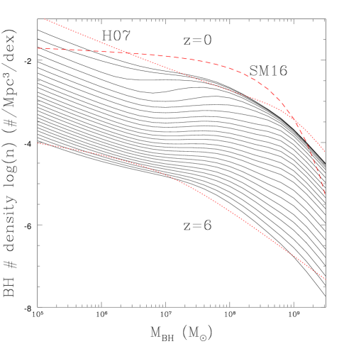
To examine the overall rates of TDEs we need the black hole mass function $n(M_{BH})$ as a function of redshift. We consider the models of Hopkins et al. (2007) and Shankar et al. (2009), focusing on the more recent Shankar et al. (2009) models. Both models are based on using quasar luminosity functions and estimates of merger rates to model the growth of black holes, constrained by the requirement of matching local estimates of the black hole mass function. The Shankar et al. (2009), mass function is defined per (base 10) logarithmic mass interval, $n(M_{BH})=dn/d\log M_{BH}$, over the mass range $5.0<\log M_{BH}/M_{\odot}<9.6$ and the redshift range $0<z<6$ as shown in Figure 1. The number of lower mass black holes is divergent ($\sim M_{BH}^{-3/2}$ for low $M_{BH}$), although the total mass in black holes is convergent. This means that the observed rate of TDEs from low mass black holes is controlled by selection effects. Strubbe & Quataert (2009) used the Hopkins et al. (2007) models and these are very similar, as illustrated by their structure at $z=0$ and $6$ in Figure 1. Mageshwaran & Mangalam (2015) used an evolving quasar luminosity function rescaled by a duty cycle estimate, while Stone & Metzger (2016) start from a local galaxy luminosity function and then populate the galaxies with black holes using the McConnell & Ma (2013) bulge/black hole mass correlation combined with a bulge mass-dependent black hole occupation fraction. This mass function, which has a shallower divergence $\sim M_{BH}^{-1.07}$ for low black hole masses, is also shown in Figure 1. As emphasized by Stone & Metzger (2016), the degree to which the divergence of the number density for small $M_{BH}$ is real controls the absolute volumetric rate of TDEs.

Some properties of TDEs may depend on the orbital pericentric radius $R_{p}$ relative to the nominal disruption radius $R_{T}$, usually expressed as the ratio $\beta=R_{T}/R_{p}$. Since we are simply adopting $\eta=1$ in Equation 1, $\beta$ is restricted to the range $1<\beta<\beta_{m}$ where

$$\beta_{m}={R_{T}\over R_{S}}=5.1R_{*1}M_{*1}^{-1/3}M_{BH7}^{-2/3}$$ (6)

is the point where the star passes through the horizon (arguably, we could also use the last stable orbit). The distribution of encounters in $\beta$ is non-trivial and cannot simply be derived from the $r\propto R_{T}^{1/4}$ scaling of Equation 3. If Equation 3 really was directly related to the distribution of pericentric radii for disrupting stars, it would imply an unphysical differential distribution of $dP/dR_{p}\propto R_{p}^{-3/4}$ that is dominated by strongly radial orbits. The same holds for the $dP/dR_{p}\propto 1/R_{p}$ distribution adopted by Strubbe & Quataert (2009).

TDE rates are dominated by two limiting regimes (see, e.g., Wang & Merritt 2004). For more distant orbits, the orbital angular momentum changes relative to the scale needed to pass close to the black hole faster than the orbital time scale. In this “pinhole” limit, the angular momentum for an encounter is random. For closer orbits, the angular momentum changes slowly compared to the orbital time scale. In this “diffusion” limit, an orbit slowly approaches the critical angular momentum needed to reach $R_{T}$. In the “pinhole” limit, $dP/dR_{p}$ is constant once we include the effects of gravitational focusing, and thus $dP/d\beta\propto\beta^{-2}$ (e.g., Luminet & Barbuy 1990). In the diffusion limit, all stars disrupt very close to $R_{T}$, so $dP/dR_{p}\propto\delta(R_{p}-R_{T})$ and $dP/d\beta\propto\delta(\beta-1)$. Following Stone & Metzger (2016) we model this as

$${dP\over d\beta}\simeq\left\{\begin{array}[]{ll}f_{pin}\beta^{-2}\left(1-\beta_{m}^{-1}\right)&1<\beta\leq\beta_{m}\\ \left(1-f_{pin}\right)&\beta=1\end{array}\right.$$ (7)

where a reasonable match to their estimates of the fraction of “pinhole” mergers is

$$f_{pin}\simeq\left(1+M_{BH7}^{1/2}\right)^{-1}.$$ (8)

Low mass black holes have core structures favoring encounters closer than $R_{T}$ in addition to having large $\beta_{m}$, allowing such encounters while remaining outside the black hole.

The importance of $\beta=R_{T}/R_{p}$ is presently under discussion. The simplest physical picture of a TDE is that the star reaches pericenter intact and then is disrupted with a spread in orbital binding energy set by the tides across the star,

$$\delta\epsilon\simeq{GM_{BH}R_{*}\over R_{T}^{2}}\beta^{n}$$ (9)

with $R_{S}\leq R_{p}\leq R_{T}$ ($1\leq\beta\leq\beta_{m}=R_{T}/R_{S}$) and $n=2$ (following Stone et al. 2013). However, Guillochon & Ramirez-Ruiz (2013) (also see Hayasaki et al. 2013) found that this was not the case in their numerical simulations and that the spread in energy was essentially independent of $\beta$, implying $n=0$. This was further confirmed by the semi-analytical study of Stone et al. (2013). In essence, the star ceases to be bound as it crosses $R_{T}$ and the debris already proceeding on independent orbits before it approaches pericenter.

The consequence of $n=0$ rather than $n=2$ can be seen in how the energy spread then determines the characteristic fall back time,

$$t_{fb}=0.36\beta^{-3n/2}M_{BH7}^{1/2}m_{*1}^{-1}R_{*1}^{3/2}~{}\hbox{years}.$$ (10)

For a given fall back time, there is a characteristic peak accretion rate of $\dot{M}_{peak}=M_{*}c^{2}/3t_{fb}$. Compared to the Eddington rate, this accretion rate is

$${\dot{M}_{peak}\over\dot{M}_{E}}\simeq 4.4\beta^{3n/2}M_{BH7}^{-3/2}M_{*1}^{2}R_{*1}^{-3/2},$$ (11)

assuming a radiative efficiency of $\eta=10\%$ ($L=\eta\dot{M}c^{2}$). This is an overestimate of the accretion rate if only (part of) the envelope is stripped, as can occur for evolved stars (see MacLeod et al. 2012). There is a big difference between the $n=2$ scaling, where close encounters produce short ($t_{fb}\propto\beta^{-3}$), high peak accretion rate events ($\dot{M}_{peak}\propto\beta^{3}$), and $n=0$, where the time scale and peak accretion rates are independent of $\beta$.

For surveys, the discovery of a TDE largely depends on $t_{fb}$ and $\dot{M}_{peak}$ – the rise time must be short enough to trigger a detection, and the peak luminosity must be high enough to allow detection of events in a large enough volume. Overall event durations for TDEs are long enough to be unimportant factors for discovery. If $n=2$, the importance of “pinhole” encounters is greatly enhanced. First, events with long $t_{fb}$ at $\beta=1$ become short enough to trigger a transient survey. Second, and more importantly, if peak luminosities determine detectability and scale as $L_{peak}\propto\dot{M}_{peak}\propto\beta^{3}$, then the survey volume scales as $V\propto L_{peak}^{3/2}\propto\beta^{9/2}$. Since $dN/d\beta\propto\beta^{-2}$, the contribution of events at a given $\beta$ scales as $dr/d\beta\propto VdN/d\beta\propto\beta^{1/2}$ and events with $\beta\simeq\beta_{m}$ (modulo the Eddington limit) will dominate the observed rates. If, on the other hand, $n=0$, then the time scales and peak luminosities are independent of $\beta$ and the relative detectability of events with differing $\beta$ must depend on higher order effects than the basic time and accretion rate scales. To avoid considering too many cases, we will follow Guillochon & Ramirez-Ruiz (2013), Stone et al. (2013) and Stone & Metzger (2016) and assume $n=0$ for our primary discussion in §3. We illustrate some consequences of $n=2$ in the Appendix.

If we focus on the UV/optical TDEs, the observed optical/UV spectra are broadly consistent with black bodies (Holoien et al. 2014, Holoien et al. 2016), although the turn over at short wavelengths is not always observed and it is clear that some TDEs with thermal optical/UV properties have significant non-thermal emission components (Holoien et al. 2016). The general assumption for these events is that the observed emission is reprocessed emission from an underlying accretion disk (e.g., Loeb & Ulmer 1997, Strubbe & Quataert 2009, Guillochon et al. 2014, Strubbe & Murray 2015, Stone & Metzger 2016) rather than direct emission from an accretion disk (e.g., Strubbe & Quataert 2009, Lodato & Rossi 2011), although other hypotheses have been advanced (e.g., Svirski et al. 2015). To the extent this is true and the observed temperature is hot compared to typical survey bands (e.g. V-band for ASAS-SN), the observed peak luminosity is

$$\left(\nu L_{\nu}\right)_{peak}=\epsilon L_{peak}{15\over\pi^{4}}\left({h\nu\over kT_{peak}}\right)^{3}$$ (12)

where $\epsilon$ is some dimensionless efficiency factor. This reprocessing model is different from Lodato & Rossi (2011), where the optical emission is the tail of direct emission from an accretion disk. To the extent that $T_{peak}$ does not vary wildly as a systematic function of parameters ($M_{BH}$, $\beta$, etc.), and $L_{peak}$ is Eddington limited, then there is a very simple model for the relative survey volumes to be associated with different events. If an Eddington limited event from a $M_{BH}=10^{7}M_{\odot}$ black hole would be detected in a local survey out in volume $V_{0}$, then any other event would be detected in volume

$${V\over V_{0}}=\left({\min\left(\dot{M}_{peak},\dot{M}_{E}(M_{BH})\right)\over\dot{M}_{E}(10^{7}M_{\odot})}\right)^{3/2}.$$ (13)

This provides a simple approach to reasonably estimating the differential contributions of events to a survey, while avoiding the very much harder problem of determining $L_{peak}$/$T_{peak}$ and hence the volume $V_{0}$ in which the fiducial event would be detectable. More importantly, $V_{0}$ can simply be estimated empirically from the properties of observed transients, as we will do crudely for the ASAS-SN survey in §3.3. Equation 13 is appropriate for low redshift surveys like ASAS-SN where cosmology and evolution can be neglected. Other effects may also suppress the observed contributions from lower mass black holes. For example, Stone & Metzger (2016) explore a model where only relatively close encounters ($R_{p}<6R_{S}$) circularize the debris rapidly and produce a strong flare, which means that only high $\beta$ pinhole encounters contribute to the TDE rate as $M_{BH}$ decreases below $\sim 10^{7}M_{\odot}$.

Figure 2: Integral TDE rates, $r(>M_{*})$, per black hole as a function of stellar mass $M_{*}$ for black hole mass ranges of $10^{8.5}$-$10^{9.5}$ (top left), $10^{7.5}$-$10^{8.5}$ (top right), $10^{6.5}$-$10^{7.5}$ (lower left), $10^{5.5}$-$10^{6.5}$ (lower left) and either 1 Gyr burst (black, solid) or constant (red, dashed) star formation models. The present ages (from most to fewest higher mass stars) are 1, 3 and 10 Gyr. The two star formation models are identical at 1 Gyr.

Figure 3: Differential TDE rates, $dr/d\log M_{*}$, per black hole as a function of stellar mass $M_{*}$ for black hole mass ranges of $10^{8.5}$-$10^{9.5}$ (top left), $10^{7.5}$-$10^{8.5}$ (top right), $10^{6.5}$-$10^{7.5}$ (lower left), $10^{5.5}$-$10^{6.5}$ (lower left) and either 1 Gyr burst (black, solid) or constant (red, dashed) star formation models. The present ages (from most to fewest higher mass stars) are 1, 3 and 10 Gyr. The two star formation models are identical at 1 Gyr.

Figure 4: Rates per black hole for different stellar evolutionary phases as a function of black hole mass for the 1 Gyr burst model at 3 Gyr (top left) or 10 Gyr (top right) and the continuous star formation model at 3 Gyr (lower left) or 10 Gyr (lower right). The red dashed line shows the total rate, and the solid lines show (from top to bottom) the rates for MS stars, sub-giants, red giant and later evolutionary states and horizontal branch and later evolutionary states. The two points with error bars are the rate estimates by van Velzen & Farrar (2014) (vV14) and Holoien et al. (2016) (H16). Their location in black hole mass is in the range of the BH mass estimates for observed TDEs.

Figure 5: Integral distribution $n(>f_{MS})$ of main sequence stars in the fraction of elapsed main sequence lifetime $f_{MS}$ at disruption for black hole mass ranges of $10^{6.5}$-$10^{7.5}$ (black lower/left) and $10^{7.5}$-$10^{8.5}M_{\odot}$ (red, upper/right). The solid curves are for the 1 Gyr burst model at 1 (lower), 3 (middle) and 10 Gyr (top), and the dashed curves are for the constant star formation model at 3 (lower) and 10 Gyr (top). The distributions are normalized to $n(>f_{MS}=0)=1$ but the upper halves of the distributions are not shown to make the distribution near $f_{MS}=1$ more visible.

3 TDE Demographics

In this section we explore various aspects of the demographics of TDEs. In §3.1 we examine the effects of the star formation history on the masses and evolutionary states of the disrupted stars as a function of black hole mass. In §3.2 we examine the effects changing the scaling of the capture rates in Equation 5 with black hole mass. In §3.3 we survey the properties of local TDEs in stellar mass, evolutionary state, peak accretion rate ($\dot{M}_{peak}/\dot{M}_{E}$), fall-back time ($t_{fb}$) and pericentric distance ($\beta=R_{T}/R_{p}$). In §3.4 we examine the evolution of TDE rates with redshift.

3.1 Stellar Mass and Evolutionary State

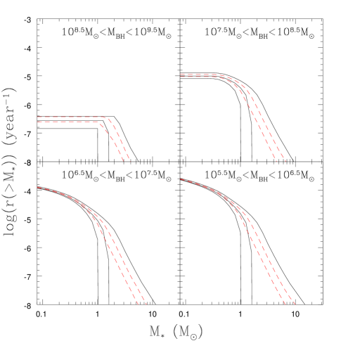
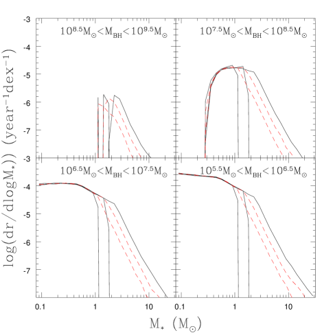
Figures 2 and 3 show the integral, $r(>M_{*})$, and differential, $dr/d\log M_{*}$, TDE rates as a function of stellar mass for black hole mass bins centered at $M_{BH}=10^{6}$, $10^{7}$, $10^{8}$, and $10^{9}M_{\odot}$ and the two star formation histories (a 1 Gyr burst or constant) at ages of $1$, $3$ and $10$ Gyr. At 1 Gyr, the two star formation histories are identical. The rate estimates at $M_{BH}\sim 10^{6}M_{\odot}$ of roughly $10^{-4}$ year^-1 are consistent with earlier results, as they must be given their underlying dependence on the Wang & Merritt (2004) models.

For the two lower black hole mass ranges, the rates are dominated by lower mass, main sequence stars, as was already well known. The rates increase slightly towards lower black hole masses because of the weak black hole mass dependence of Equation 5. Because the Kroupa (2001) mass function is almost logarithmically flat at low masses and it is somewhat easier to disrupt higher mass, lower mean density main sequence stars, the logarithmic rates are almost constant for $M_{*}<0.5M_{\odot}$ and then drop slowly up to $M_{*}\simeq M_{\odot}$ due to the break in the slope of the IMF. The typical TDE is of an $M_{*}\simeq 0.3M_{\odot}$ main sequence M-dwarf. The star formation history completely controls the rates for higher mass stars, but affects the total rates little since only 14% of stars on the IMF have $M_{*}>M_{\odot}$. The rapid decline in stellar lifetimes with stellar mass leads to very sharp breaks in the mass dependent rates for the burst star formation models at late times.

In the next higher mass range, centered on $M_{BH}=10^{8}M_{\odot}$, we begin to see the effects of the dropping strength of the tidal gravity at the event horizon as the black hole mass increases. The lower mass M dwarfs can no longer be disrupted, leading to an order of magnitude drop in the TDE rate. The mass function of the disrupted stars is strongly truncated near $M_{*}\simeq 0.3M_{\odot}$, so the typical mass of a disrupted star increases and now depends more on the star formation history. While the existence of the sharp cutoff at low masses is generic, its exact location will be sensitive to the radius used to define the boundary between disruption and absorption. Kesden (2012) explores some of these issues for rotating black holes and finds that they have only modest effects. The primary effect of the star formation history is still to modify the mass function of the disrupted stars at $M_{*}\mathrel{\raise 1.29167pt\hbox{$>$}\mkern-14.0mu\lower 2.58334pt\hbox{$\sim$}}M_{\odot}$. The total rates for the different star formation histories differ by only $\sim 25\%$.

For the highest mass black holes, the mass function of the disrupted stars and the overall rates depend strongly on the star formation history because it is increasingly only evolved stars that can undergo a TDE. The absolute rates now vary by a factor of $\sim 3$ between the star formation histories and the typical disrupted star has the mass of a star at the MS turn off. For star formation histories where the duration of the star formation period is still relevant, there is a peak with a power-law decline towards higher masses. For the older burst populations, the mass function increasingly looks like a delta function because the range of stellar ages corresponds to a negligible spread in MS turn off masses. For the higher mass black holes ($M_{BH}\mathrel{\raise 1.29167pt\hbox{$>$}\mkern-14.0mu\lower 2.58334pt\hbox{$\sim$}}10^{8}M_{\odot}$) it is likely that only the burst models are relevant at lower redshifts because the hosts will be early-type galaxies with old stellar populations.

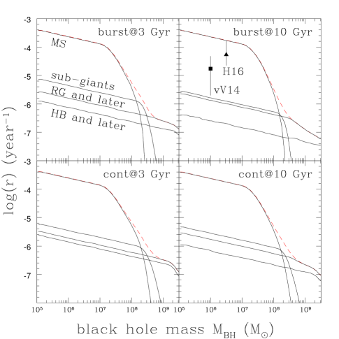
Figure 4 shows the rates as a function of the evolutionary state of the star and the black hole mass for the 3 Gyr and 10 Gyr old stellar population models. For simplicity we simply show the results for all stars, MS stars, sub-giants, stars that have evolved past the base of the RGB, and horizontal branch and later stars. MacLeod et al. (2012) illustrate relative rate distributions over these later evolutionary phases for a range of stellar masses. Figure 4 also compares the estimates to the two recent rate estimates by van Velzen & Farrar (2014) and Holoien et al. (2016). Neither study differentiates by black hole mass, but typical black hole mass estimates for observed optical/UV TDEs are of order $M_{BH}=10^{6}$ to $10^{7.5}M_{\odot}$ (see below). The two rate estimates are in mild conflict, but they illustrate the continuing tension between observed and theoretical disruption rates.

For lower black hole masses where all stars disrupt ($M_{BH}\mathrel{\raise 1.29167pt\hbox{$<$}\mkern-14.0mu\lower 2.58334pt\hbox{$\sim$}}10^{7}M_{\odot}$), the rate steadily rises for lower masses because of the $M_{BH}^{-1/4}$ scaling of the adopted rate (Equation 5). Disruptions are overwhelmingly dominated by MS stars, with evolved stars representing only $\sim 3\%$ of the rate. The rate for evolved stars is dominated by sub-giants, then red giants, and then all later phases. The average mass of the disrupted evolved stars will be much higher than the main sequence stars, so selection effects can significantly modify the observed ratios, as we will discuss in §3.3.

Starting around $M_{BH}\mathrel{\raise 1.29167pt\hbox{$>$}\mkern-14.0mu\lower 2.58334pt\hbox{$\sim$}}10^{7.5}M_{\odot}$, an increasing fraction of lower mass MS stars are absorbed rather than disrupted, leading to a very rapid drop in the TDE rate at higher black hole masses. At roughly $M_{BH}=10^{8}M_{\odot}$, the rates for evolved and MS stars are comparable, with the subgiants still dominating the rates for evolved stars. The black hole mass scale of the rapid drop in the rates will shift in direct proportion to changes in the criterion for absorption over disruption. At slightly higher black hole masses, the sub-giant contribution also drops rapidly due to a combination of two factors. First, subgiants are not tremendously larger than MS turn off stars, so for fixed stellar mass it does not take a huge increase in the black hole mass to absorb a sub-giant as compared to a MS turn off star. Second, the subgiants are associated with the highest mass MS stars in the stellar population, because the lower mass stars have not had time to evolve. As a result, the sub-giant contribution to the rates drops rapidly at masses only slightly above the black hole mass where they are as important as MS stars. Finally, as the black hole mass approaches $M_{BH}\mathrel{\raise 1.29167pt\hbox{$>$}\mkern-14.0mu\lower 2.58334pt\hbox{$\sim$}}10^{8.5}M_{\odot}$, only the giant stars contribute to the rates. Since such evolved stars are rare in all star formation histories, the expected rates are $2$ to $3$ orders of magnitude lower than for $M_{BH}\mathrel{\raise 1.29167pt\hbox{$<$}\mkern-14.0mu\lower 2.58334pt\hbox{$\sim$}}10^{7.5}M_{\odot}$ where all MS stars will be disrupted.

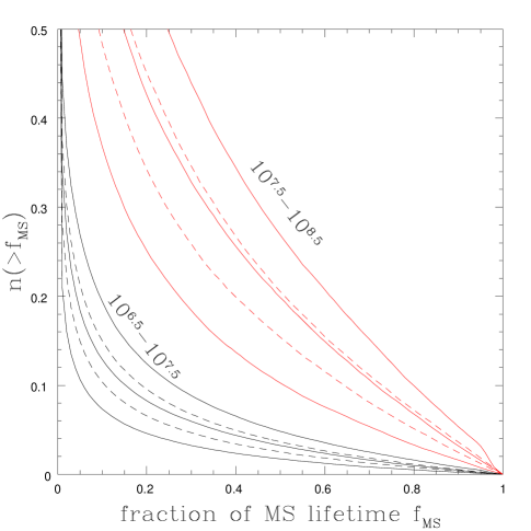
Kochanek (2015) noted that $M_{*}\mathrel{\raise 1.29167pt\hbox{$>$}\mkern-14.0mu\lower 2.58334pt\hbox{$\sim$}}M_{\odot}$ stars develop significantly depressed (enhanced) carbon (nitrogen) average abundances even by fraction $f_{MS}\simeq 0.1$ of their MS lifetime due to CNO reactions. Along with their slowly increasing helium mass fractions, this means that stellar evolution can lead to abundance anomalies in TDE debris and potentially their spectra. This is a different concern from studies of nuclear reactions triggered by deeply plunging TDE orbits (e.g., Luminet & Pichon 1989). Figure 5 shows the integral distribution $n(>f_{MS})$ for the two star formation models and ages of $1$, $3$ and $10$ Gyr for black hole mass ranges of $10^{6.5}$-$10^{7.5}$ and $10^{7.5}$-$10^{8.5}M_{\odot}$. Lower black hole mass ranges have distributions very slowly shifting to having fewer evolved stars, while higher mass black hole ranges quickly shift to being dominated by stars close to the MS turn off. For black hole masses $M_{BH}\mathrel{\raise 1.29167pt\hbox{$<$}\mkern-14.0mu\lower 2.58334pt\hbox{$\sim$}}10^{7}M_{\odot}$, the huge numbers of long lived, low mass MS stars which have had no time to evolve dominate the TDE rates. As a result only some 10-20% of MS TDEs will have significantly anomalous carbon and nitrogen abundances, and only $\sim 5\%$ will have $f_{MS}\mathrel{\raise 1.29167pt\hbox{$>$}\mkern-14.0mu\lower 2.58334pt\hbox{$\sim$}}0.5$ where the helium enhancement begins to become significant. To this can be added the $\sim 3\%$ contribution from sub-giants, which are also likely to be fully disrupted in a TDE. Later evolutionary states (aside from the rare AGB stars) are less likely to produce anomalous abundance signatures because the material inside the hydrogen burning shell is sequestered in a very high density core that is largely decoupled from the envelope. As the black hole mass increases, the fraction of TDEs associated with more evolved stars steadily increases.

Figure 6: Effects of the black hole mass function, $M_{BH}$-$\sigma$ relation and the dependence of TDE rates on $M_{BH}$ on the distribution of TDEs in black hole mass. The histogram shows the distribution of black hole mass estimates for a sample 12 optical/UV TDEs (see footnote). The solid black curve is our fiducial model based on Equation 5 and the local Shankar et al. (2009) black hole mass function. The dotted lines bracketing it show the effect of varying the logarithmic slope of the $M_{BH}$-$\sigma$ relation $M_{BH}\propto\sigma^{\alpha}$ over the range $\alpha=4.65\pm 0.50$ assuming the TDE rate scales as $\sigma^{7/2}$ as in Equation 3. Adopting the much stronger Brockamp et al. (2011) rate scalings of $r\propto M_{BH}^{0.35}$ to $M_{BH}^{0.45}$ with black hole mass does significantly alter the predictions, as shown by the black dashed lines. These are all for the 1 Gyr burst star formation model at an age of 10 Gyr.

3.2 The Local Mass Function and $M_{BH}$-$\sigma$ Relation

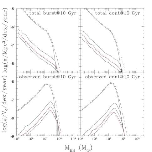
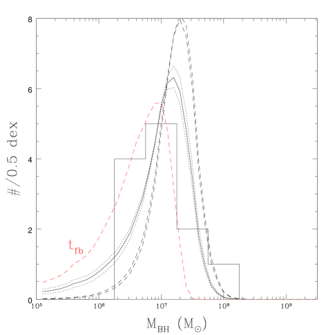
Figure 6 shows the expected distribution of local TDEs as a function of $M_{BH}$ for the 10 Gyr old burst model as a function of black hole mass for the Shankar et al. (2009) mass function. To emphasize how strongly events from low mass black holes are favored, we have used a linear scale for the numbers of events per logarithmic mass interval. The distributions are normalized for comparison to a sample of 12 optical/UV TDEs with black hole mass estimates drawn from the literature. The results for the Hopkins et al. (2007) black hole mass function are very similar.

The scaling of the rates with $M_{BH}$ in Equation 5 was something of a compromise. Many possible changes have little consequence. For example, the original rate scaling in Equation 3 depends on the bulge velocity dispersion as $\sigma^{7/2}$, which when combined with the $M_{BH}$-$\sigma$ relation $M_{BH}\propto\sigma^{4.65}$ in Equation 4 has a black hole mass dependence of $\sigma^{7/2}\propto M_{BH}^{3/4}$. Examples of other recent estimates of the exponent of the $M_{BH}$-$\sigma$ relation are $5.13$ (Graham et al. 2011), $4.32$ (Schulze & Gebhardt 2011) and $5.64$ (McConnell & Ma 2013). As also shown in Figure 6, varying the exponent of the $M_{BH}$-$\sigma$ relation by $\pm 0.5$ has very little effect on the predictions since it changes the dependence of the rate on black hole mass by a factor of only about $r\propto M_{BH}^{\pm 0.1}$. Similarly, Stone & Metzger (2016), based on McConnell & Ma (2013), used $r\propto M_{BH}^{-0.404}$, which leads to changes only slightly larger than the example of using a steeper $M_{BH}$-$\sigma$ relation.

The dominance of low mass black holes is largely driven by the relatively steep slope of the black hole mass function, ($n\propto M_{BH}^{-3/2}$ for Shankar et al. 2009), rather than the mass dependence of the rate. Even a large change in the mass dependence of the rates has difficulty suppressing the contribution from low mass black holes. For example, Brockamp et al. (2011) derive rate expressions from a series of N-body experiments that scale as $r\propto M_{BH}^{0.446}$ or $M_{BH}^{0.353}$ depending on their choice of an $M_{BH}$-$\sigma$ relation. As shown in Figure 6, this leads to a local peak near $M_{BH}\sim 10^{7}M_{\odot}$ and a reduced but still significant contribution from low mass black holes.

Without an even stronger black hole mass dependence than found by Brockamp et al. (2011), the divergence of the volumetric rates for low black hole masses is an inevitable consequence of the divergent number of low mass galaxies/halos. For the remainder of the paper we simply use our fiducial model, combining Equation 5 with the Shankar et al. (2009) black hole mass function. We show most of the subsequent distributions as a function of black hole mass, making it relatively easy to evaluate the consequences of changing either the black hole mass function or the black hole mass dependence of the TDE rates. We also examine the consequences of our simple selection effects model.

Figure 7: Volumetric (top) and observed (bottom) TDE rates as a function of stellar mass $M_{*}$ for the burst (left) and continuous (right) star formation models at an age of $10$ Gyr and the local Shankar et al. (2009) black hole mass function. In order of increasing stellar mass and diminishing TDE rates for low black hole masses, the solid curves are for $M_{*}=0.08$-$0.25$, $0.25$-$0.50$, $0.50$-$0.75$ and $0.75$-$1.0M_{\odot}$, and the dotted red curves are for $M_{*}=1.0$-$1.5$, $1.5$-$2.0$ and $>2.0M_{\odot}$. The dashed curves give the total rate. In the lower panels the rate scales with the fiducial volume $V_{0}$ (in Mpc³, see text).

Figure 8: Volumetric (top) and observed (bottom) TDE rates as a function of stellar evolutionary state for the burst (left) and continuous (right) star formation models at an age of $10$ Gyr and the local Shankar et al. (2009) black hole mass function. In order of increasing stellar age and diminishing TDE rate for low black hole masses, the solid curves are for stars with main sequence life time fractions of $f_{MS}=0$-$0.25$, $0.25$-$0.50$, $0.50$-$0.75$ and $0.75$-$1.00$ and the dotted red curves are for post-MS stars. The dashed curves give the total rate. In the lower panels the rate scales with the fiducial volume $V_{0}$ (in Mpc³, see text).

Figure 9: Volumetric (top) and observed (bottom) TDE rates as a function of the peak accretion rate in Eddington units $\dot{M}_{peak}/\dot{M}_{E}$ for the burst (left) and continuous (right) star formation models at an age of $10$ Gyr and the local Shankar et al. (2009) black hole mass function. In order of increasing accretion rate and lower black hole mass, the solid curves are accretion rates of $\dot{M}_{peak}/\dot{M}_{E}<10^{-1.5}$, $10^{-1.5}$-$10^{-1.0}$, $10^{-1.0}$-$10^{-0.5}$, and $10^{-0.5}$-$10^{0.0}$ while the dotted red curves are for accretion rates of $10^{0.0}$-$10^{0.5}$, $10^{0.5}$-$10^{1.0}$ and $>10^{1.0}$. The dashed curves show the total rate. In the lower panels the rate scales with the fiducial volume $V_{0}$ (in Mpc³, see text).

Figure 10: Volumetric (top) and observed (bottom) TDE rates as a function of the fall back time $t_{fb}$ for the burst (left) and continuous (right) star formation models at an age of $10$ Gyr and the local Shankar et al. (2009) black hole mass function. In order of increasing accretion rate and (generally) black hole mass, the solid curves are for $t_{fb}<10^{-1.5}$ years and $10^{-1.5}$-$10^{-1.0}$, while the dotted red curves are for $t_{fb}=10^{-1.0}$-$10^{-0.5}$, $10^{-0.5}$-$10^{0.0}$, $10^{0.0}$-$10^{0.5}$, $10^{0.5}$-$10^{1.0}$ and $>10^{1.0}$ years. Events with the time scales of the solid curves are very likely to trigger present day transient searches, while the time scales corresponding to the dotted red curves are increasingly likely to be ignored. Note the contribution of long time scale events for low mass black holes due to the disruption of evolved stars. The dashed curves show the total rate. In the lower panels the rate scales with the fiducial volume $V_{0}$ (in Mpc³, see text).

Figure 11: Volumetric (top) and observed (bottom) TDE rates as a function of the pericentric depth, $\beta=R_{T}/R_{p}$, of pinhole encounters for the burst (left) and continuous (right) star formation models at an age of $10$ Gyr and the local Shankar et al. (2009) black hole mass function. In order of increasing $\beta$ (smaller pericenters), the solid curves are for $\beta=1.0$-$1.5$ and $1.5$-$2.0$, while the dotted red curves are for $\beta=2$-$4$, $4$-$8$ and $>8$. The dashed curves show the total rate. The overall rates must be modified by the fraction of pinhole relative to diffusive encounters (e.g. Equation 8). In the lower panels the rate scales with the fiducial volume $V_{0}$ (in Mpc³, see text).

3.3 Local Demographics

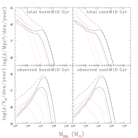
Next we explore the distribution of TDE properties as a function of black hole mass for the local Shankar et al. (2009) mass function and (as limiting cases) the burst and continuous star formation models at an age of 10 Gyr. The results for other star formation histories can be approximately inferred from the earlier figures including all 5 star formation histories. In each case, we show the “true” volumetric rate per logarithmic black hole mass interval and the “observed” rate per unit fiducial volume $V_{0}$ (in Mpc³) assuming that $n=0$ so that high $\beta$ disruptions have the same fall back times and peak luminosities as those at $\beta\simeq 1$ (see the discussion in §2 and the Appendix).

As a reminder, the fiducial volume $V_{0}$ is nominally the volume in which an Eddington-limited TDE for a $10^{7}M_{\odot}$ black hole would be detected. We are simply going to give a rough empirical calibration based on the ASAS-SN TDEs (Holoien et al. 2014, Holoien et al. 2016), which are associated with black holes roughly in this mass range and have peak luminosities that are reasonably close to the Eddington limit. For example, ASASSN-14ae (Holoien et al. 2014) had an observed peak of $M_{V}\simeq-19.5$ mag (the true peak was likely slightly higher). ASAS-SN can detect such transients out to a comoving distance of roughly 200 Mpc and monitors roughly one-third of the sky after clipping the Galactic plane and fields that are just rising or setting. Thus, a reasonable, empirical estimate for the ASAS-SN survey is that $V_{0}\simeq 10^{7}$ Mpc³. This is meant to provide a rough guide for interpreting rates rather than as a formal estimate.

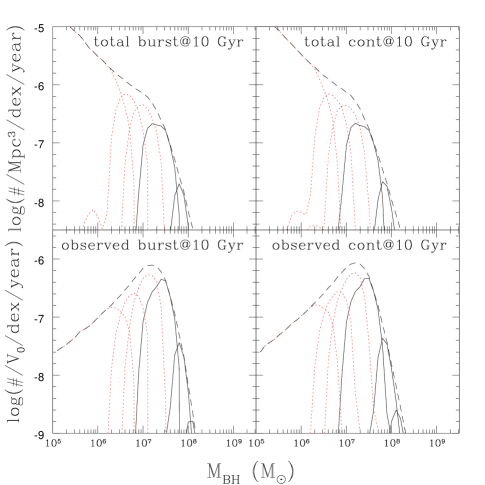
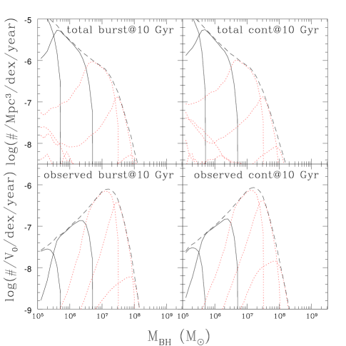
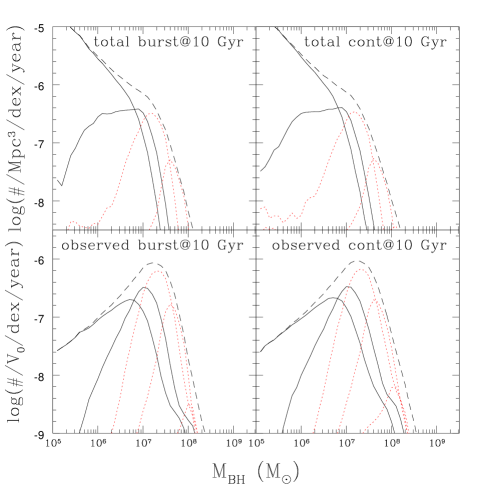
First, in Figures 7 and 8, we show the distributions in stellar mass and evolutionary state. In the volumetric rates, we again see that the low mass dwarfs completely dominate the rates for $M_{BH}\mathrel{\raise 1.29167pt\hbox{$<$}\mkern-14.0mu\lower 2.58334pt\hbox{$\sim$}}10^{7}M_{\odot}$, and then the dominant mass rapidly shifts to higher stellar masses as lower mass stars are absorbed rather than captured. For the highest mass black holes, the volumetric rates are driven by the $M_{*}\mathrel{\raise 1.29167pt\hbox{$>$}\mkern-14.0mu\lower 2.58334pt\hbox{$\sim$}}M_{\odot}$ stars, but only the continuous star formation models have any events from stars significantly more massive than $M_{*}\simeq M_{\odot}$. For our simple selection effects model (Equation 13), the observed contributions from lower mass black holes are strongly suppressed because the Eddington limit on the luminosity restricts the survey volume, $V\propto L_{Edd}^{3/2}\propto M_{BH}^{3/2}$. The contribution at high masses is suppressed by the steeply falling mass function (Figure 1) and because the longer fall back time scales and roughly fixed stellar masses increasingly limit the accretion rate to be below Eddington. As a result, the observed events are strongly peaked near $10^{7}M_{\odot}$ rather than having the distribution of Figure 6.

Similarly, as long as the rates are dominated by the low mass dwarfs, most TDEs are from stars that are very young compared to their overall MS lifetimes. The contribution from stars past the mid-point of their MS lifetimes is nearly $\sim 30$ times lower, For these lower mass black holes, the contributions from post-main sequence stars and stars near the end of their MS lifetimes are comparable. As the dwarfs are increasingly absorbed rather than disrupted for higher mass black holes, the distribution of events in stellar age becomes much more uniform. And then, finally, the TDEs associated with the highest mass black holes are increasingly due to evolved stars. In the observed distributions, the balance is modestly shifted towards older stars as the fall back time scales become longer and the numerous low mass dwarfs can no longer support Eddington-limited accretion. In both the stellar mass and evolutionary state distributions, the differences between the burst and continuous star formation models are relatively subtle, with obvious differences only for high mass black holes where the TDE rates are dominated by evolved stars.

Figure 9 and 10 show the distributions of events in peak accretion rate, $\dot{M}_{peak}/\dot{M}_{E}$, and fall-back time, $t_{fb}$, assuming $n=0$ in Equations 10 and 11. In a volume limited sample of TDEs, the spread in the black hole masses is so large compared to the spread in stellar masses that there is a tight correlation of $\dot{M}_{peak}/\dot{M}_{E}$ with $M_{BH}$ even when a stellar mass function is included. Lower mass black holes have higher accretion rates, and Figure 9 may underestimate the trend because we simply used $M_{*}$ for the disruptions of evolved stars (rather than a partial stripping model, e.g., MacLeod et al. 2012). If, however, the luminosities are Eddington limited, then the visibility of the high $\dot{M}_{peak}/\dot{M}_{E}$ events associated with lower mass black holes is greatly reduced, and the sample of observed TDEs will be fairly tightly clustered around $\dot{M}_{peak}/\dot{M}_{E}\sim 1$.

With the simple selection effects model, the expected observed TDE rate is roughly $1.5\times 10^{-6}V_{0}$/year. Given our rough estimate of $V_{0}\simeq 10^{7}$ Mpc³ for ASAS-SN, this implies a TDE rate in ASAS-SN of order 15/year. In practice, ASAS-SN is finding roughly one TDE per year (Holoien et al. 2014, Holoien et al. 2016). One possibility is that our TDE model is overestimating the rate by an order of magnitude, but the distribution in fall back times seen in Figure 10 suggests an alternate explanation.

The fall back time is largely set by the black hole mass, and spans a range from 10 days or less at $M_{BH}=10^{5}M_{\odot}$ up to decades at $10^{9}M_{\odot}$. If we consider the four lowest time scale bins in Figure 10, $t_{fb}<10^{-1.5}$, $10^{-1.5}$-$10^{-1.0}$, $10^{-1.0}$-$10^{-0.5}$ and $10^{-0.5}$-$10^{0.0}$ years ($<12$ days, 12-37 days, 37-116 days and 116-365 days) they contain roughly 2%, 14%, 61%, 22% and 1% of the observed events. To the extent that the fall back time is a reasonable proxy for event rise times, it is likely that most transient surveys will increasingly reject sources with time scales longer than $t_{fb}>10^{-1.0}$ years that are located at the centers of galaxies because of AGN variability and other potential false positives. If we required $t_{fb}<10^{-1.0}$ years as a selection limit, we would have only 16% of the potentially observable TDEs, leading to a rate of only $2.5$/year in ASAS-SN that is far more compatible with observed discovery rate. This is not a panacea since such a cut on the time scales truncates the expected black hole mass distribution at a somewhat lower black hole mass than observed (compare Figures 6 and 10). Raising the limit on the time scale to $t_{fb}<10^{-0.75}$ years (65 days) quickly reintroduces the rate tension, with an expected rate in ASAS-SN of order 6.7/year. Nonetheless, the existence of selection effects related to the fall back time scale seems inevitable.

If such a limit on the fall back time scale is needed to reconcile the observed and predicted rates, then it is probably also necessary for the arguments by Guillochon & Ramirez-Ruiz (2013) and Stone et al. (2013) that encounters with $\beta>1$ have similar time scales to those with $\beta=1$ to be correct. In the Appendix (Figure 16), we show the consequences of scaling the fall back time with the depth of the encounter ($n=2$ in Equation 10). The distribution of pinhole events across the four lowest time scale bins is now 26%, 24%, 41% and 8%, which is a significant shift towards shorter time scales. While this would be diluted by the fraction of encounters that are diffusive (Equation 8), using $n=2$ would make it much more difficult (impossible?) to use time scale selection effects to reduce the observed contribution from higher mass black holes.

Finally, Figure 11 shows the distribution in the depth of the encounter, $\beta=R_{T}/R_{p}$, as a function of black hole mass for the pinhole encounters. This would then be diluted by the fraction $1-f_{pin}(M)$ (Equation 8) of orbits driven by diffusion to disrupt at $\beta\simeq 1$. For $M_{BH}\mathrel{\raise 1.29167pt\hbox{$>$}\mkern-14.0mu\lower 2.58334pt\hbox{$\sim$}}10^{7}M_{\odot}$, the vast majority of pinhole encounters disrupt relatively close to the tidal limit, with $\beta\mathrel{\raise 1.29167pt\hbox{$<$}\mkern-14.0mu\lower 2.58334pt\hbox{$\sim$}}2$. Only for relatively low mass black holes are there significant numbers of deeply plunging orbits. The number of plunging encounters in a volume limited sample is then significantly lower because the Eddington limit greatly suppresses the survey volume for the lower mass black holes. This would not change if we used $n=2$ instead of $n=0$, so that the plunging encounters would have significantly shorter fall back times and peak mass accretion rates (Equations 10 and  11), because the luminosities produced by these low black hole masses are already Eddington-limited. We explore this issue further in the Appendix.

Figure 12: The evolution of the comoving TDE rate with redshift for all stars (upper curves) and non-MS stars (lower curves). The standard burst (solid) and continuous (dashed) star formation models are shown, where the younger models produce more evolved star TDEs. The total rates are shown for both the Shankar et al. (2009) (S09, black) and Hopkins et al. (2007) (H07 red) black hole mass functions. The “mergers” curve shows the result for a TDE rate driven by mergers with a merger rate scaled by the inverse of the age of the universe, $t_{H}(z)^{-1}$, and normalized to equal the contribution of isolated black holes at $z=0$. The square point and error bar show the volumetric rate estimate by van Velzen & Farrar (2014) located at the mean redshift of the two candidate TDEs in their sample. The triangle and error bar shows the Holoien et al. (2016) rate implied by simply maintaining the rate ratio relative to van Velzen & Farrar (2014). The stellar populations are not evolved with redshift for simplicity since they have so little effect on the overall rates compared to the evolution of the black hole mass function.

Figure 13: Expected distribution of observed TDEs in black hole mass given our simple model for selection effects. As in Figure 6, the histogram shows the distribution of black hole mass estimates for a sample of 12 optical/UV TDEs. The solid black curve is our fiducial model based on Equation 5 and the local Shankar et al. (2009) black hole mass function. The observed distribution can be well-explained by selection effects despite the divergence of the total volumetric rate at low black hole mass. The dotted lines bracketing it show the effect of varying the logarithmic slope of the $M_{BH}$-$\sigma$ relation $M_{BH}\propto\sigma^{\alpha}$ over the range $\alpha=4.65\pm 0.50$ assuming the rate scales as $\sigma^{7/2}$ as in Equation 3. Adopting the much stronger Brockamp et al. (2011) rate scalings of $r\propto M_{BH}^{0.35}$ to $M_{BH}^{0.45}$ with black hole mass does significantly alter the predictions, as shown by the black dashed lines. The red dashed curve labeled $t_{fb}$ shows an example of the effect of excluding events with long fall back times from the standard model (see text). These are all for the burst star formation model at an age of 10 Gyr.

Figure 14: The evolution of the comoving TDE rate with redshift in black hole mass bins of $M_{BH}=10^{5}$-$10^{6}M_{\odot}$ (top), $M_{BH}=10^{6}$-$10^{7}M_{\odot}$, $M_{BH}=10^{7}$-$10^{8}M_{\odot}$, and $M_{BH}>10^{8}M_{\odot}$ (bottom) for the Shankar et al. (2009) black hole mass function. The standard burst (solid) and continuous (dashed) star formation models are shown, where the younger models produce more evolved star TDEs. The red curves show the effect on the volumetric rate of excluding events with long fall back times from the standard model for the $M_{BH}=10^{6}$-$10^{7}M_{\odot}$, and $M_{BH}=10^{7}$-$10^{8}M_{\odot}$ mass bins (see text). The point and error bar show the volumetric rate estimate by van Velzen & Farrar (2014) located at the mean redshift of the two candidate TDEs in their sample.

3.4 The Evolution of TDE Rates With Redshift

The final issue we explore is the evolution of TDE rates with redshift. This was incorporated in the Strubbe & Quataert (2009) models using the Hopkins et al. (2007) model for the black hole mass function. Strubbe & Quataert (2009) noted that the rates are predicted to decline with increasing redshift but did not explore the issue in any detail. For simplicity, we will not attempt to simultaneously evolve the stellar populations with the black hole mass functions. We know from the earlier sections that the effects of star formation histories on the rates are small compared to the rapid changes in the black hole mass function with cosmic epoch seen in Figure 1. We will show results for the various star formation histories, and the consequences of adding any evolution can be understood by simply interpolating between curves.

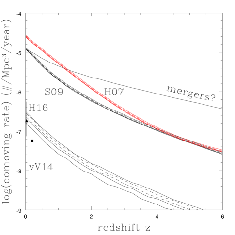
Figure 12 shows evolution of the rates integrated over the $10^{5}M_{\odot}<M_{BH}<10^{9.6}M_{\odot}$ mass range spanned by the Shankar et al. (2009) models. The absolute rates are limited by the cutoff in the mass functions at $M_{BH}=10^{5}M_{\odot}$ because of the steep low mass slope of the mass function (see Figure 1). With the estimated rates dropping by a factor of 5 even by $z=1$, TDEs are clearly creatures of the local universe. The Hopkins et al. (2007) black hole mass function, shown only for the total rates in Figure 12, predicts a moderately higher local rate and a similar decline with redshift.

For comparison, we also show the volumetric rate estimate by van Velzen & Farrar (2014) located at the mean redshift ($\langle z\rangle=0.20$) of the two candidate TDEs ($z=0.136$ and $z=0.256$, van Velzen et al. 2011). Like their estimated rate per black hole, their observational estimate is low compared to our theoretical model (and previous models). Holoien et al. (2016) did not estimate a volumetric rate, but the mean redshift of the ASAS-SN TDEs is significantly lower ($\langle z\rangle=0.032$). We can approximately convert their rate to a volumetric rate by simply assuming that the ratio of the volumetric rates between Holoien et al. (2016) and van Velzen & Farrar (2014) is the same as the ratio of the rates per galaxy shown in Figure 4. This rescaling is roughly consistent with ASAS-SN finding roughly 1 TDE/year in a survey volume of roughly $V_{0}=10^{7}$ Mpc³ (the estimate we used in §3.3). The difference between these estimates (whatever the flaws) is consistent with the rapid evolution of TDE rates even if the absolute scale differs from the models by a large factor.

That the observed TDEs tend to have $M_{BH}\mathrel{\raise 1.29167pt\hbox{$>$}\mkern-14.0mu\lower 2.58334pt\hbox{$\sim$}}10^{6}M_{\odot}$ (see Figure 6) suggests that the contributions from the lower mass systems that dominate the theoretical rates either do not exist because the mass functions are wrong or because these events are being missed due to selection effects. Figure 13 reprises the $M_{BH}$ distribution in Figure 6 after including our simple model for selection effects. Despite the divergence of the volumetric rates towards lower masses, the concentration of the observed TDEs near $M_{BH}\simeq 10^{7}M_{\odot}$ is well-reproduced. The divergence of the mass function ($dn/dM_{BH}\sim M_{BH}^{-3/2}$) is balanced by the reduction in the survey volume associated with the Eddington limit ($V\propto M_{BH}^{+3/2}$) leaving a distribution $dr/d\log M_{BH}\propto M_{BH}^{3/4}$ for low black hole masses. Given the uncertainties in black hole masses, the modest offset between the model and observed peaks is probably not significant.

Figure 13 also shows the consequences of adding a selection limit on $t_{fb}$ to the standard model based on the discussion in §3.3. We use a detection probability of unity for $t_{fb}<10^{-1.0}$ years, zero for $t_{fb}>10^{-0.5}$ years and a linear transition in $\log t_{fb}$ in between. This model better matches the peak of the observed TDEs and is still statistically compatible with observing no lower mass black holes in the observed sample (although not by much). It is not compatible with the presence of the higher mass black holes in the observed sample. Given that black hole mass estimates are logarithmically uncertain at the level of $\sim 0.5$ dex, one solution would be to argue that the high mass tail is simply due to scatter in the mass estimates. Alternatively, we could change the $t_{fb}$ selection model to cut off at somewhat longer time scales or only drop to a finite floor instead of zero. Given the available data, it presently seems sufficient to simply present an example of the consequences of including a time scale selection effect.

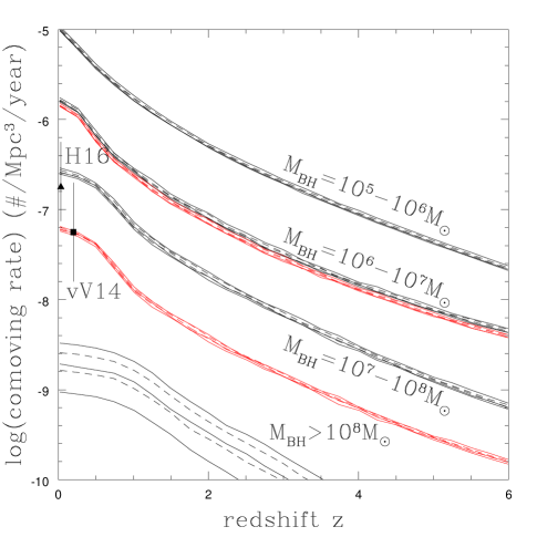
An alternative view of the role of the black hole mass function is shown in Figure 14. Here we show the rate contributed by four different bins of black hole mass. The radical disagreement between the theoretical and van Velzen & Farrar (2014) or the (scaled) Holoien et al. (2016) rates in Figure 12 is dominated by the contribution from the $M_{BH}=10^{5}$-$10^{6}M_{\odot}$ bin. The differences between the observed rates and those for the $M_{BH}=10^{6}$-$10^{7}M_{\odot}$ black hole mass bin, where the bulk of the observed TDEs appear to lie (see Figure 6 and 13), are significantly smaller. There is again the huge drop off in rates above $M_{BH}\mathrel{\raise 1.29167pt\hbox{$>$}\mkern-14.0mu\lower 2.58334pt\hbox{$\sim$}}10^{8}M_{\odot}$. The black hole mass dependence of the TDE rates recapitulates the phenomenon of “downsizing”, where the contribution from higher mass black holes stops increasing rapidly towards lower redshifts earlier than for lower mass black holes.

Figure 14 also shows the effects of adding our simple selection limit on $t_{fb}$ for the $M_{BH}=10^{6}$-$10^{7}M_{\odot}$ and $M_{BH}=10^{7}$-$10^{8}M_{\odot}$ mass bins (it has no effect on the lowest mass bin and eliminates all the very high mass events, so these are not shown). While adding this limit greatly suppresses the rates for the higher mass black holes, it does not have a significant effect on the rates for the $M_{BH}=10^{6}$-$10^{7}M_{\odot}$ mass range. Shifting the $t_{fb}$ limits to sufficiently short time scales would greatly reduce the rates for this lower mass bin, but would greatly exacerbate the tension between the observed and predicted black hole mass distributions discussed earlier.

Finally, Arcavi et al. (2014) (also see French et al. 2016) noted that a surprising number of TDEs seem to be in post-starburst galaxies (a.k.a. E$+$A or K$+$A galaxies), suggesting that TDE rates may be significantly boosted after a merger. Mergers could do so through two mechanisms. The first possible mechanism is that the orbital diffusion time scales are significantly shorter for an extended period of time after a merger. Presumably, mergers do rapidly refill loss cones, essentially by shifting from orbital evolution driven by relaxation to evolution driven by violent relaxation. A second, more likely mechanism, is that the post-starburst phase is also the period when the black holes associated with the mergers are themselves merging. For example, Li et al. (2015) find that TDE rates can be enhanced by two orders of magnitude in the phases before the system becomes a compact binary, although this phase does not last 1 Gyr.

For present purposes, we need no detailed knowledge of the mechanism to explore the possible consequences of mergers for the evolution of the rates of TDEs. Besides the “reference” model we have used here, Shankar et al. (2009) considered models with mergers. For merger rates which were relatively high, there was little effect until $z<1$ where growth by accretion begins to slow. Then at lower redshifts, the mergers drove the black hole mass function to be more dominated by high mass black holes, a difference which would tend to reduce the TDE rate. In the Shankar et al. (2009) models, the rate of mergers is independent of black hole mass and proportional to the inverse of the age of the universe, $t_{H}(z)^{-1}$. This means that the TDE rate contributed by mergers approximately evolves as $r(z)t_{H}(0)/t_{H}(z)$, where we approximate $r(z)$ using the fiducial, no merger model of Shankar et al. (2009) since the model with mergers was not tabulated. Figure 12 shows how such a contribution to the TDE rate would evolve with redshift, normalized to match the reference model at $z=0$. The TDE rate still drops with redshift, but more slowly because the decrease in the absolute numbers of black holes (Figure 1) is partly balanced by the increasing rate of mergers.

4 Discussion

As already known, TDE rates should be dominated by the disruption of low mass ($M_{*}\mathrel{\raise 1.29167pt\hbox{$<$}\mkern-14.0mu\lower 2.58334pt\hbox{$\sim$}}M_{\odot}$), main sequence stars by black holes of modest mass, $M_{BH}\mathrel{\raise 1.29167pt\hbox{$<$}\mkern-14.0mu\lower 2.58334pt\hbox{$\sim$}}10^{7.5}M_{\odot}$. In detail, the mass function of disrupted lower mass stars is fairly flat because the slope of the stellar mass function is partly balanced by the lower densities of higher mass stars. Some $\sim 10\%$ of disrupted stars are high enough mass for the CNO cycle to be relevant and have lived long enough ($f_{MS}\mathrel{\raise 1.29167pt\hbox{$>$}\mkern-14.0mu\lower 2.58334pt\hbox{$\sim$}}10\%$ of their main sequence lifetime) to show depressed carbon and enhanced nitrogen abundances, as discussed in Kochanek (2015). Smaller numbers of older ($f_{MS}\mathrel{\raise 1.29167pt\hbox{$>$}\mkern-14.0mu\lower 2.58334pt\hbox{$\sim$}}50\%$) main sequence stars and subgiants will show significant increases in their average helium abundance. For higher mass black holes, where the lowest mass stars are increasingly absorbed rather than disrupted, the typical mass and age of the disrupted star increases rapidly. Above roughly $M_{BH}\mathrel{\raise 1.29167pt\hbox{$>$}\mkern-14.0mu\lower 2.58334pt\hbox{$\sim$}}10^{8.5}M_{\odot}$, only evolved stars are disrupted. The detailed star formation history is not very important except for the the rates associated with $M_{*}\mathrel{\raise 1.29167pt\hbox{$>$}\mkern-14.0mu\lower 2.58334pt\hbox{$\sim$}}M_{\odot}$ or evolved stars and high mass black holes.

The black hole mass function is the crucial factor in determining TDE rates because simple models of black hole growth and evolution (e.g. Hopkins et al. 2007, Shankar et al. 2009) predict diverging numbers of lower mass black holes just as there are diverging numbers of low mass halos or galaxies. Stone & Metzger (2016) explored this in a more empirical model based on simply adding black holes to a galaxy luminosity function and then simply truncating the mass function below some limiting black hole mass. For our black hole mass functions, which extend down to $10^{5}M_{\odot}$, the disagreement between the model and observed rates (e.g., van Velzen & Farrar 2014, Holoien et al. 2016) is large (factor of $\sim 30$). One possibility, explored by Stone & Metzger (2016), is that the black hole mass function is simply truncated below $M_{BH}\mathrel{\raise 1.29167pt\hbox{$<$}\mkern-14.0mu\lower 2.58334pt\hbox{$\sim$}}10^{6}M_{\odot}$.

A second possibility is that selection effects are strongly affecting the observed rates. Even with a diverging mass function, TDEs due to low mass black holes are almost certainly associated with lower peak luminosities and hence smaller survey volumes. With small numbers of known TDEs, this can quickly lead to discovering no examples of the most common events and hence gross underestimates of the true volumetric rates. In particular, the observed distribution of optical/UV TDE black hole masses is cut off at low black hole masses in agreement with our simple model for survey selection effects. The model also predicts that the observed sample should be dominated by somewhat higher mass black holes than observed, and this is may be explained by a selection bias against surveys examining slowly rising transients at the centers of galaxies. Combining these selection effects appears to largely, but not perfectly, reconcile the observed and theoretical rates. Searching for TDEs with longer time scales in somewhat more massive galaxies is likely to be profitable.

The typical accretion rates associated with TDEs are of order $10^{-5}$ to $10^{-4}M_{\odot}$ year^-1, very similar to the estimate by Magorrian & Tremaine (1999). Even without any dramatic evolution in the rates, this means that the net contribution of TDEs to the mean mass of a black holes is $10^{5}$ to $10^{6}M_{\odot}$. Only for low mass black holes is this rate high enough to significantly contribute to their growth. However, the contribution to the growth of the lower mass black holes comes from disrupted stars rather than absorbed stars, and it increasingly appears that most (all?) TDEs accrete very little of the available mass (see, e.g., the discussion in Metzger & Stone (2015)). If 10% or less of the mass is actually accreted, then the TDE process quickly becomes unimportant for the growth of even the lower mass black holes. These estimates also assume that the total mass of the star is disrupted – for evolved stars with large core/envelope density differences, it is likely that only the envelope is lost (or portions of the envelope, see, e.g., MacLeod et al. 2012).

In the Hopkins et al. (2007) and Shankar et al. (2009) models for the evolution of the black hole mass function, TDE rates are predicted to drop very rapidly with redshift, falling by a factor of $\sim 5$ by a redshift of unity. The effect is largest for the lowest mass black holes, in a TDE version of “downsizing”. The evolution is so rapid, that it could explain a significant fraction of the factor of $\sim 3$ nominal rate difference between van Velzen & Farrar (2014) at $z\simeq 0.2$ and Holoien et al. (2016) at $z\simeq 0.03$. Although it is also true that the two rate estimates are sufficiently uncertain to be mutually consistent without the rapid redshift evolution. Without a well-established model for the behavior of TDEs as a function of mass that can be used to model selection effects, it may prove difficult to use TDEs to probe the black hole mass function as proposed by Stone & Metzger (2016). Since the evolution with redshift at fixed black hole mass is predicted to be so rapid and TDE properties at fixed black hole mass are unlikely to evolve rapidly, it should be considerably easier to test models for the evolution of the black hole mass function with redshift using TDEs. For example, the slowly evolving theoretical black hole mass function of Sijacki et al. (2015) used by Metzger et al. (2015) to predict the rates of jetted TDEs should be easily distinguishable from the more empirical and rapidly evolving models of Hopkins et al. (2007) and Shankar et al. (2009).

While the volumetric rates, which depend on the black hole mass function, show the largest mismatch to observational estimates, there may still be significant discrepancies between predicted and observed rates per galaxy. Any problems have to lie in the rate estimates more than uncertainties in other aspects of the estimates such as the choice of $M_{BH}$-$\sigma$ relations. There is less of an issue if the higher rates found by Holoien et al. (2016), (as compared to van Velzen & Farrar (2014), for example) are correct. There are, for example, fundamental differences between the rate estimates by Wang & Merritt (2004) or their updates in Stone & Metzger (2016) and the estimates of Brockamp et al. (2011). In the former estimates, the TDE rate declines with black hole mass ($\propto M_{BH}^{-0.16}$ to $\propto M_{BH}^{-0.40}$), while in the latter estimates, the rate increases with black hole mass ($\propto M_{BH}^{0.35}$ to $M_{BH}^{0.45}$). Since the range of black hole masses spans 4-5 dex or more, such large differences in the mass scaling will have an enormous impact on the mass-dependent rates. In particular, the rapid rise in the rate with black hole mass found by Brockamp et al. (2011) greatly suppresses the rate contribution of even a divergent population of low mass black holes.

More broadly, the semi-empirical rate estimates based on the observed structures of galaxies (e.g. Magorrian & Tremaine 1999, Wang & Merritt 2004, Stone & Metzger 2016), are essentially all for galaxies containing black holes above $M_{BH}\mathrel{\raise 1.29167pt\hbox{$>$}\mkern-14.0mu\lower 2.58334pt\hbox{$\sim$}}10^{6}M_{\odot}$. Part of the problem is the difficulty in identifying systems with lower mass black holes (see, e.g., Greene & Ho 2007). Independent of this problem, present extrapolations of TDE rates to lower black hole masses assume an extrapolation of the dynamical structure of the host galaxies to lower mass hosts. The degree to which this is valid is an open question, as illustrated by the ongoing debates about bulges, pseudo-bulges, and black holes (see, e.g., Kormendy & Ho 2013, Kormendy 2016, for reviews of some of the issues). Detailed models of loss cone dynamics for these lower mass galaxies are required.

If post-starburst galaxies produce a significant fraction of TDEs (Arcavi et al. 2014, French et al. 2016), then the standard rate estimates are unlikely to be applicable to these systems. Many of the TDE properties explored in this paper may be little affected. At least in the survey of such galaxies by Quintero et al. (2004), the luminosity function of post-starburst galaxies is almost identical in shape to the luminosity function of all galaxies – roughly 1% of galaxies at all luminosities show the strong Balmer absorption features characterizing this class of galaxy. This suggests that the black hole mass function of such galaxies is similar to that of all galaxies, and that just the TDE rate is being accelerated. However, secondary issues (e.g. mass-dependent black hole merger rates if the rate increase is due to binary black holes) could then modulate the mass dependence of the rates. Of course, the fundamental tension between the predicted and observed rates is only exacerbated if many of the observed TDEs are due to a different mechanism than the standard loss cone mechanism.

On the observational side, the key issue is the extent to which the observed properties of TDEs and their hosts are dominated by selection effects. Understanding this requires transient surveys to be sensitive to TDEs with (rise) time scales of many months to years in order to probe higher black hole masses. If the suggestion by Kochanek (2015) that nitrogen rich quasars may be related to TDEs is correct, than surveys for spectral evolution in (particularly the nitrogen rich) quasars may be an alternate probe for higher mass TDEs. Transient surveys are generally sensitive to the much shorter time scales expected for lower mass systems, and may just be limited by reduced survey volumes because lower mass black holes have lower peak luminosity transients. Alternatively, if TDE phenomenology (e.g., X-ray, UV or optically dominated) depends strongly on black hole mass, then it will be necessary to unify the results of all the different search strategies used to date.

Appendix A Pinhole Encounters When $n=2$

Figure 15: Volumetric (top) and observed (bottom) TDE rates as a function of the peak accretion rate in Eddington units $\dot{M}_{peak}/\dot{M}_{E}$ for pinhole encounters with $n=2$ so that the peak accretion rate increases with the depth of the encounter as $\dot{M}_{peak}/\dot{M}_{E}\propto\beta^{3}$ (see Equation 11). This Figure should be compared to Figure 9. In order of increasing accretion rate and black hole mass, the solid curves are accretion rates of $\dot{M}_{peak}/\dot{M}_{E}<10^{-1.5}$, $10^{-1.5}$-$10^{-1.0}$, $10^{-1.0}$-$10^{-0.5}$, and $10^{-0.5}$-$10^{0.0}$ while the dotted red curves are for accretion rates of $10^{0.0}$-$10^{0.5}$, $10^{0.5}$-$10^{1.0}$ and $>10^{1.0}$. The dashed curves show the total rate. In the lower panels the rate scales with the fiducial volume $V_{0}$ (in Mpc³, see text).

Figure 16: Volumetric (top) and observed (bottom) TDE rates as a function of the fall back time $t_{fb}$ for pinhole encounters with $n=2$ so that the fall back time decreases with the depth of the encounter as $t_{fb}\propto\beta^{-3}$ (see Equation 10. This Figure should be compared to Figure 10. In order of increasing accretion rate and (generally) black hole mass, the solid curves are for $t_{fb}<10^{-1.5}$ years and $10^{-1.5}$-$10^{-1.0}$, while the dotted red curves are for $t_{fb}=10^{-1.0}$-$10^{-0.5}$, $10^{-0.5}$-$10^{0.0}$, $10^{0.0}$-$10^{0.5}$, $10^{0.5}$-$10^{1.0}$ and $>10^{1.0}$ years. Events with the time scales of the solid curves are very likely to trigger present day transient searches, while the time scales corresponding to the dotted red curves are increasingly likely to be ignored. Note the contribution of long time scale events for low mass black holes due to the disruption of evolved stars. The dashed curves show the total rate. In the lower panels the rate scales with the fiducial volume $V_{0}$ (in Mpc³, see text).

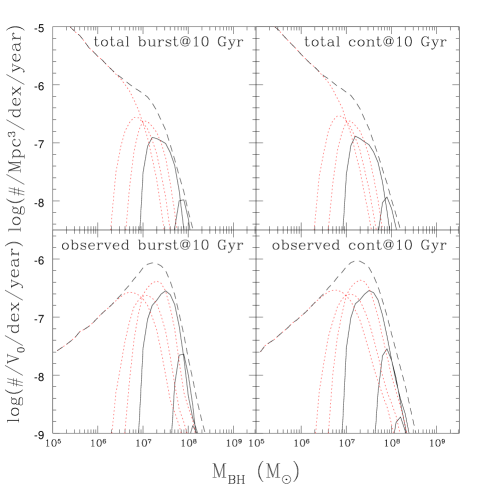
As discussed in §2, if the energy spread produced during an encounter is relatively independent of the pericenter ($n=0$), then the depth of the encounter $\beta=R_{T}/R_{p}$ becomes a secondary variable because the basic time time and accretion scales are independent of $\beta$. Figures 15 and 16 show how the distributions of pinhole events in $\dot{M}/\dot{M}_{E}$ and $t_{fb}$ change compared to Figures 9 and 10 if we use $n=2$ for Equations 11 and 10 instead of $n=0$. The peak accretion rates and fall back times now increase as $\beta^{3}$ and decrease as $\beta^{-3}$ respectively, where $\beta=R_{T}/R_{p}$ characterizes the depth of the pericentric radius $R_{p}$ compared to the tidal radius $R_{T}$ (Equation 1). The range is limited to $R_{T}/R_{S}<\beta<1$ with the probability distribution of Equation 7. The overall distribution would then have to average over the fraction of pinhole and diffusive events (Equation 8).

Very roughly speaking, the consequence of using $n=2$ is that the typical accretion rate at fixed $M_{BH}$ increases by roughly $0.5$ dex and the typical fall back time decreases by roughly $0.5$ dex. The accretion rate at the peak of the expected observed rate distribution is now mildly super-Eddington, and the typical fall back time scale is closer to one month than three months. These shifts would exacerbate many of the tensions in the rates and black hole mass distributions, particularly since it makes it more difficult to argue that some of the differences can be explained by transient surveys tending to ignore longer time scale variability at the centers of galaxies.

References

- Arcavi et al. (2014) Arcavi, I., Gal-Yam, A., Sullivan, M., et al. 2014, ApJ, 793, 38
- Belczynski et al. (2010) Belczynski, K., Bulik, T., Fryer, C. L., et al. 2010, ApJ, 714, 1217
- Bonnerot et al. (2016) Bonnerot, C., Rossi, E. M., Lodato, G., & Price, D. J. 2016, MNRAS, 455, 2253
- Brockamp et al. (2011) Brockamp, M., Baumgardt, H., & Kroupa, P. 2011, MNRAS, 418, 1308
- Cannizzo et al. (1990) Cannizzo, J. K., Lee, H. M., & Goodman, J. 1990, ApJ, 351, 38
- Carter & Luminet (1983) Carter, B., & Luminet, J.-P. 1983, AAP, 121, 97
- Chen et al. (2008) Chen, X., Liu, F. K., & Magorrian, J. 2008, ApJ, 676, 54
- Chornock et al. (2014) Chornock, R., Berger, E., Gezari, S., et al. 2014, ApJ, 780, 44
- Cohn & Kulsrud (1978) Cohn, H., & Kulsrud, R. M. 1978, ApJ, 226, 1087
- Dai et al. (2013) Dai, L., Escala, A., & Coppi, P. 2013, ApJL, 775, L9
- Donley et al. (2002) Donley, J. L., Brandt, W. N., Eracleous, M., & Boller, T. 2002, AJ, 124, 1308
- Evans & Kochanek (1989) Evans, C. R., & Kochanek, C. S. 1989, ApJL, 346, L13
- French et al. (2016) French, K. D., Arcavi, I., & Zabludoff, A. 2016, arXiv:1601.04705
- Gezari et al. (2006) Gezari, S., Martin, D. C., Milliard, B., et al. 2006, ApJL, 653, L25
- Gezari et al. (2008) Gezari, S., Basa, S., Martin, D. C., et al. 2008, ApJ, 676, 944
- Gezari et al. (2009) Gezari, S., Heckman, T., Cenko, S. B., et al. 2009, ApJ, 698, 1367
- Gezari (2012) Gezari, S. 2012, European Physical Journal Web of Conferences, 39, 03001
- Gezari et al. (2012) Gezari, S., Chornock, R., Rest, A., et al. 2012, Nature, 485, 217
- Graham et al. (2011) Graham, A. W., Onken, C. A., Athanassoula, E., & Combes, F. 2011, MNRAS, 412, 2211
- Greene & Ho (2007) Greene, J. E., & Ho, L. C. 2007, ApJ, 667, 131
- Guillochon & Ramirez-Ruiz (2013) Guillochon, J., & Ramirez-Ruiz, E. 2013, ApJ, 767, 25
- Guillochon et al. (2014) Guillochon, J., Manukian, H., & Ramirez-Ruiz, E. 2014, ApJ, 783, 23
- Hayasaki et al. (2013) Hayasaki, K., Stone, N., & Loeb, A. 2013, MNRAS, 434, 909
- Hills (1975) Hills, J. G. 1975, Nature, 254, 295
- Holoien et al. (2014) Holoien, T. W.-S., Prieto, J. L., Bersier, D., et al. 2014, MNRAS, 445, 3263
- Holoien et al. (2016) Holoien, T. W.-S., Kochanek, C. S., Prieto, J. L., et al. 2016, MNRAS, 455, 2918
- Hopkins et al. (2007) Hopkins, P. F., Richards, G. T., & Hernquist, L. 2007, ApJ, 654, 731
- Kaiser et al. (2002) Kaiser, N., Aussel, H., Burke, B. E., et al. 2002, SPIE, 4836, 154
- Kalirai et al. (2008) Kalirai, J. S., Hansen, B. M. S., Kelson, D. D., et al. 2008, ApJ, 676, 594
- Kasen & Ramirez-Ruiz (2010) Kasen, D., & Ramirez-Ruiz, E. 2010, ApJ, 714, 155
- Kesden (2012) Kesden, M. 2012, PRD, 85, 024037
- Kochanek (1994) Kochanek, C. S. 1994, ApJ, 422, 508
- Kochanek (2015) Kochanek, C. S. 2015, MNRAS, 446, 1213
- Komossa (2015) Komossa, S. 2015, arXiv:1505.01093
- Kormendy (2016) Kormendy, J. 2016, Galactic Bulges, 418, 431
- Kormendy & Ho (2013) Kormendy, J., & Ho, L. C. 2013, ARA&A, 51, 511
- Kreidberg et al. (2012) Kreidberg, L., Bailyn, C. D., Farr, W. M., & Kalogera, V. 2012, ApJ, 757, 36
- Kroupa (2001) Kroupa, P. 2001, MNRAS, 322, 231
- Lacy et al. (1982) Lacy, J. H., Townes, C. H., & Hollenbach, D. J. 1982, ApJ, 262, 120
- Law et al. (2009) Law, N. M., Kulkarni, S. R., Dekany, R. G., et al. 2009, PASP, 121, 1395
- Li et al. (2015) Li, S., Liu, F. K., Berczik, P., & Spurzem, R. 2015, arXiv:1509.00158
- Lightman & Shapiro (1977) Lightman, A. P., & Shapiro, S. L. 1977, ApJ, 211, 244
- Lodato et al. (2009) Lodato, G., King, A. R., & Pringle, J. E. 2009, MNRAS, 392, 332
- Lodato & Rossi (2011) Lodato, G., & Rossi, E. M. 2011, MNRAS, 410, 359
- Loeb & Ulmer (1997) Loeb, A., & Ulmer, A. 1997, ApJ, 489, 573
- Luminet & Pichon (1989) Luminet, J.-P., & Pichon, B. 1989, AAP, 209, 85
- Luminet & Barbuy (1990) Luminet, J.-P., & Barbuy, B. 1990, AJ, 99, 838
- MacLeod et al. (2012) MacLeod, M., Guillochon, J., & Ramirez-Ruiz, E. 2012, ApJ, 757, 134
- Mageshwaran & Mangalam (2015) Mageshwaran, T., & Mangalam, A. 2015, ApJ, 814, 141
- Magorrian & Tremaine (1999) Magorrian, J., & Tremaine, S. 1999, MNRAS, 309, 447
- Marigo et al. (2008) Marigo, P., Girardi, L., Bressan, A., et al. 2008, AAP, 482, 883
- McConnell & Ma (2013) McConnell, N. J., & Ma, C.-P. 2013, ApJ, 764, 184
- Merritt & Wang (2005) Merritt, D., & Wang, J. 2005, ApJL, 621, L101
- Metzger et al. (2015) Metzger, B. D., Williams, P. K. G., & Berger, E. 2015, ApJ, 806, 224
- Metzger & Stone (2015) Metzger, B. D., & Stone, N. C. 2015, arXiv:1506.03453
- Miller (2015) Miller, M. C. 2015, ApJ, 805, 83
- Özel et al. (2010) Özel, F., Psaltis, D., Narayan, R., & McClintock, J. E. 2010, ApJ, 725, 1918
- Pfuhl et al. (2011) Pfuhl, O., Fritz, T. K., Zilka, M., et al. 2011, ApJ, 741, 108
- Piran et al. (2015) Piran, T., Svirski, G., Krolik, J., Cheng, R. M., & Shiokawa, H. 2015, ApJ, 806, 164
- Quintero et al. (2004) Quintero, A. D., Hogg, D. W., Blanton, M. R., et al. 2004, ApJ, 602, 190
- Rees (1988) Rees, M. J. 1988, Nature, 333, 523
- Sadowski et al. (2015) Sadowski, A., Tejeda, E., Gafton, E., Rosswog, S., & Abarca, D. 2015, arXiv:1512.04865
- Schulze & Gebhardt (2011) Schulze, A., & Gebhardt, K. 2011, ApJ, 729, 21
- Shankar et al. (2009) Shankar, F., Weinberg, D. H., & Miralda-Escudé, J. 2009, ApJ, 690, 20
- Shappee et al. (2014) Shappee, B. J., Prieto, J. L., Grupe, D., et al. 2014, ApJ, 788, 48
- Shiokawa et al. (2015) Shiokawa, H., Krolik, J. H., Cheng, R. M., Piran, T., & Noble, S. C. 2015, ApJ, 804, 85
- Sijacki et al. (2015) Sijacki, D., Vogelsberger, M., Genel, S., et al. 2015, MNRAS, 452, 575
- Svirski et al. (2015) Svirski, G., Piran, T., & Krolik, J. 2015, arXiv:1508.02389
- Smartt et al. (2009) Smartt, S. J., Eldridge, J. J., Crockett, R. M., & Maund, J. R. 2009, MNRAS, 395, 1409
- Stone et al. (2013) Stone, N., Sari, R., & Loeb, A. 2013, MNRAS, 435, 1809
- Stone & Metzger (2016) Stone, N. C., & Metzger, B. D. 2016, MNRAS, 455, 859
- Strubbe & Quataert (2009) Strubbe, L. E., & Quataert, E. 2009, MNRAS, 400, 2070
- Strubbe & Quataert (2011) Strubbe, L. E., & Quataert, E. 2011, MNRAS, 415, 168
- Strubbe & Murray (2015) Strubbe, L., & Murray, N., 2015, MNRAS in press [arXiv:1509.04277]
- Syer & Ulmer (1999) Syer, D., & Ulmer, A. 1999, MNRAS, 306, 35
- van Velzen et al. (2011) van Velzen, S., Farrar, G. R., Gezari, S., et al. 2011, ApJ, 741, 73
- van Velzen & Farrar (2014) van Velzen, S., & Farrar, G. R. 2014, ApJ, 792, 53
- Vasiliev & Merritt (2013) Vasiliev, E., & Merritt, D. 2013, ApJ, 774, 87
- Wang & Merritt (2004) Wang, J., & Merritt, D. 2004, ApJ, 600, 149
- Wang et al. (2012) Wang, T.-G., Zhou, H.-Y., Komossa, S., et al. 2012, ApJ, 749, 115