11institutetext: Daniel Hug 22institutetext: Karlsruhe Institute of Technology, Institute of Stochastics, D-76128 Karlsruhe, 22email: daniel.hug@kit.edu 33institutetext: Michael A. Klatt 44institutetext: Karlsruhe Institute of Technology, Institute of Stochastics, D-76128 Karlsruhe, 44email: michael.klatt@kit.edu 55institutetext: Günter Last 66institutetext: Karlsruhe Institute of Technology, Institute of Stochastics, D-76128 Karlsruhe, 66email: guenter.last@kit.edu 77institutetext: Matthias Schulte 88institutetext: Karlsruhe Institute of Technology, Institute of Stochastics, D-76128 Karlsruhe, 88email: matthias.schulte@kit.edu

Second order analysis of geometric functionals of Boolean models

Daniel Hug    Michael A. Klatt    Günter Last    Matthias Schulte
Abstract

This paper presents asymptotic covariance formulae and central limit theorems for geometric functionals, including volume, surface area, and all Minkowski functionals and translation invariant Minkowski tensors as prominent examples, of stationary Boolean models. Special focus is put on the anisotropic case. In the (anisotropic) example of aligned rectangles, we provide explicit analytic formulae and compare them with simulation results. We discuss which information about the grain distribution second moments add to the mean values.

1 Introduction

In this article we study a large class of functionals of the Boolean model, a fundamental benchmark model of stochastic geometry CSKM13 ; SchneiderWeil ; Molchanov1996 and continuum percolation Hall1988 ; MeesterRoy96 . It has many applications in material science Torquato.2002 , physics Arns.2003 ; ScholzEtAl2015 , and astronomy Buchert.1994 ; Kerscher.2001 , as well as, for the measurement of biometrical data Mecke.2005 or the estimation of percolation thresholds Mecke.1991 ; Mecke.2002b . Intuitively speaking, a Boolean model is a collection of overlapping random grains, scattered in space in a purely random manner. This random object is defined as follows. Let X={X1,X2,}𝑋subscript𝑋1subscript𝑋2X=\{X_{1},X_{2},\ldots\} be a stationary Poisson process of intensity γ𝛾\gamma in nsuperscript𝑛{\mathbb{R}}^{n}, that is, a countable collection of random points in nsuperscript𝑛{\mathbb{R}}^{n} such that the numbers of points in disjoint sets are independent and the number of points in each set follows a Poisson distribution whose parameter is γ𝛾\gamma times the Lebesgue measure of the set. Let (Zi)isubscriptsubscript𝑍𝑖𝑖(Z_{i})_{i\in\mathbb{N}} be a sequence of independent and identically distributed random convex bodies (nonempty compact convex subsets of nsuperscript𝑛{\mathbb{R}}^{n}), independent of X𝑋X. The Boolean model Z𝑍Z is the random closed set defined by

Z:=i(Zi+Xi),assign𝑍subscript𝑖subscript𝑍𝑖subscript𝑋𝑖Z:=\bigcup_{i\in\mathbb{N}}(Z_{i}+X_{i}),

where Zi+Xi:={z+Xi:zZi}assignsubscript𝑍𝑖subscript𝑋𝑖conditional-set𝑧subscript𝑋𝑖𝑧subscript𝑍𝑖Z_{i}+X_{i}:=\{z+X_{i}:z\in Z_{i}\}. An example is the spherical Boolean model, where the Zisubscript𝑍𝑖Z_{i} are balls with random radii centred at the origin and Zi+Xisubscript𝑍𝑖subscript𝑋𝑖Z_{i}+X_{i} is the corresponding ball centred at Xisubscript𝑋𝑖X_{i}.

In this paper we study geometric functionals of the Boolean model Z𝑍Z. Prominent examples of such functionals are the intrinsic volumes (Minkowski functionals) and Minkowski tensors, which are efficient shape descriptors that have been successfully applied to a variety of physical systems SchroederTurketal2011AdvMater . (In SchroederTurketal2013NJP , the different approaches and notations in the physics and mathematics literature are compared.). We are interested in the second order properties of the random variables obtained by applying geometric functionals to the restriction ZW𝑍𝑊Z\cap W of the Boolean model to a convex observation window Wn𝑊superscript𝑛W\subset{\mathbb{R}}^{n}. For a stationary and isotropic Boolean model, Miles Miles76 and Davy Davy76 obtained explicit formulae expressing the mean values of the Minkowski functionals in terms of the intensity and geometric mean values of the typical grain (see also CSKM13 ; SchneiderWeil ). For mean value formulae for more general functionals in Boolean models we refer to HoerrmannWeil2016 . We shall discuss here formulae for asymptotic covariances as well as multivariate central limit theorems for an increasing observation window. Much of the presented theory is taken from HLS . However, some results are new. In particular this is the first paper providing explicit covariance formulae involving the Euler characteristic of planar non-isotropic Boolean models. Our methods are based on the Fock space representation of Poisson functionals from LaPe11 and the Stein-Malliavin approach to their normal approximation Peccatietal2010 ; LPS16 ; LastPenrose . A completely different treatment of second moments of curvature measures of an isotropic Boolean model with an interesting application to morphological thermodynamics was presented in Mecke01 . There, two different scenarios are considered: first, a Poisson distributed number of grain centres in the observation window (Poisson process), and second, a fixed number of grains (Binomial process). In statistical physics, these two choices are called the grand canonical and the canonical ensemble. The second moments of geometric quantities show a similar behaviour as thermodynamical quantities in statistical physics Mecke01 ; Mecke2000 . For the perfectly isotropic examples of overlapping discs or spheres, the covariances of the Minkowski functionals are also discussed in BrMe2002 or Kerscher.2001 , respectively.

This paper is organized in the following way. After introducing Boolean models and geometric functionals in Section 2, Section 3 is devoted to the covariance structure of geometric functionals of Boolean models. First, we present general covariance formulae. Then, we concentrate on planar Boolean models. Univariate and multivariate central limit theorems for geometric functionals of Boolean models are discussed in Section 4. In Section 5, we explicitly compute the covariance formulae for a special Boolean model of aligned rectangles. In the final Section 6, we present and discuss simulation results for Boolean models with rectangles and compare them with our theoretical findings. The agreement is excellent.

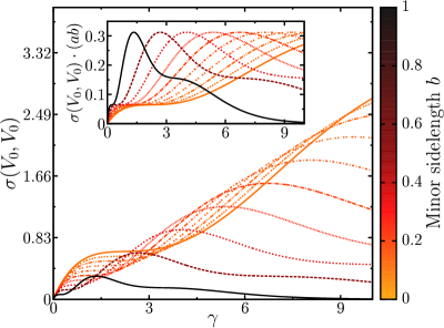
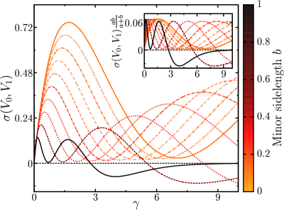
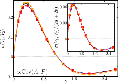
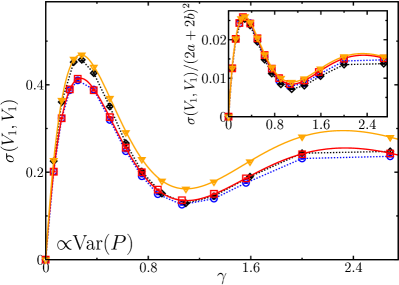
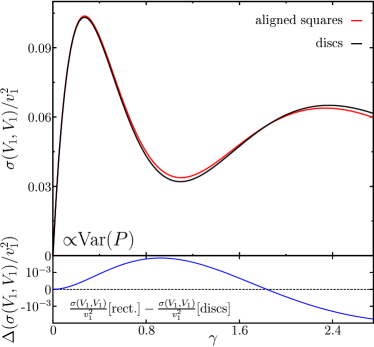
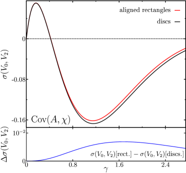
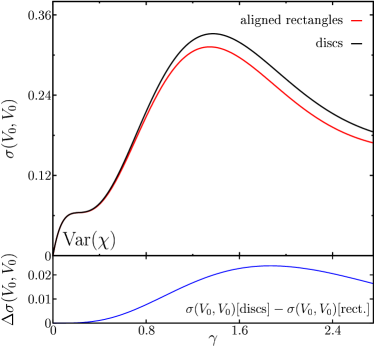
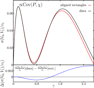
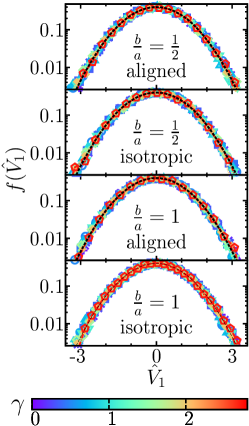
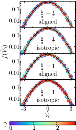
Let us finish this introduction with an informal summary of our results for applied scientists. We calculate for certain models of disordered systems of overlapping grains the second moments of a quite general class of robust shape descriptors, which include as well-known examples volume, surface area, Euler characteristic, and, more generally, all Minkowski functionals and tensors. Our results apply to general anisotropic grain distributions, see Theorems 3.2 and 3.3. The anisotropic case of aligned (planar) rectangles is discussed in great detail; see Section 5 and Fig. 2. It is interesting to note that the asymptotic formulae for the infinite volume system are actually exact for finite systems with periodic boundary conditions; see Subsection 3.3. The central limit theorem for the geometric functionals (see Theorems 4.1 and 4.2) ascertains that in the limit of infinite system size the probability distributions of the normalized geometric functionals are normal distributions. If the structure of a given sample is reasonably well described by the (joint) cumulative probability distributions of the geometric functionals, it is possible to construct tests of certain model hypotheses for random heterogeneous media based on the asymptotic normality and our explicit covariance formulae. We discuss the behaviour of the second moments (e.g., how they differ for various models) and probability distributions in finite systems for specific examples: either aligned or isotropically oriented rectangles (distributed randomly in space). Moreover, we derive explicit formulae (see Fig. 2) and compare the results to simulations (see Figs. 3 and 5).

2 Preliminaries

In the introduction we have defined a Boolean model in terms of a stationary Poisson process in nsuperscript𝑛{\mathbb{R}}^{n} which is independently marked with random convex bodies, see, e.g., HoerrmannWeil2016 . In this paper we use an equivalent description based on a Poisson process in the space 𝒦nsuperscript𝒦𝑛{\mathcal{K}}^{n} of convex bodies. For our purposes this representation is more convenient.

We equip 𝒦nsuperscript𝒦𝑛{\mathcal{K}}^{n} with its Borel σ𝜎\sigma-field (𝒦n)superscript𝒦𝑛\mathcal{B}({\mathcal{K}}^{n}) with respect to the Hausdorff metric. We call a measure ΘΘ\Theta on 𝒦nsuperscript𝒦𝑛{\mathcal{K}}^{n} locally finite if

Θ({K𝒦n:KC})<,C𝒞n,formulae-sequenceΘconditional-set𝐾superscript𝒦𝑛𝐾𝐶𝐶superscript𝒞𝑛\Theta(\{K\in{\mathcal{K}}^{n}:K\cap C\neq\emptyset\})<\infty,\quad C\in\mathcal{C}^{n},

where 𝒞nsuperscript𝒞𝑛\mathcal{C}^{n} is the space of compact subsets of nsuperscript𝑛{\mathbb{R}}^{n}. Let 𝐍𝐍\mathbf{N} be the space of all locally finite counting measures on 𝒦nsuperscript𝒦𝑛{\mathcal{K}}^{n} and let it be equipped with the smallest σ𝜎\sigma-field 𝒩𝒩\mathcal{N} such that all maps νν(A)maps-to𝜈𝜈𝐴\nu\mapsto\nu(A), A(𝒦n)𝐴superscript𝒦𝑛A\in\mathcal{B}({\mathcal{K}}^{n}), from 𝐍𝐍\mathbf{N} to {0,}0\mathbb{N}\cup\{0,\infty\} are measurable. Each element ν𝐍𝜈𝐍\nu\in\mathbf{N} has a representation

ν=i=1NδKi,K1,K2,𝒦n,N{0,},formulae-sequence𝜈superscriptsubscript𝑖1𝑁subscript𝛿subscript𝐾𝑖subscript𝐾1subscript𝐾2formulae-sequencesuperscript𝒦𝑛𝑁0\nu=\sum_{i=1}^{N}\delta_{K_{i}},\quad K_{1},K_{2},\ldots\in{\mathcal{K}}^{n},\quad N\in\mathbb{N}\cup\{0,\infty\},

where δKsubscript𝛿𝐾\delta_{K} stands for the Dirac measure concentrated at K𝒦n𝐾superscript𝒦𝑛K\in{\mathcal{K}}^{n}. Because of this representation one can think of ν𝜈\nu as a countable collection of convex bodies (or grains).

Throughout this paper all random objects are defined on a fixed (sufficiently rich) probability space (Ω,𝒜,𝐏)Ω𝒜𝐏(\Omega,{\mathcal{A}},{\mathbf{P}}). We call a random element η𝜂\eta in 𝐍𝐍\mathbf{N} a Poisson process with a locally finite intensity measure ΘΘ\Theta if

  1. (i)

    η(A1),,η(Am)𝜂subscript𝐴1𝜂subscript𝐴𝑚\eta(A_{1}),\ldots,\eta(A_{m}) are independent for disjoint sets A1,,Am(𝒦n)subscript𝐴1subscript𝐴𝑚superscript𝒦𝑛A_{1},\ldots,A_{m}\in\mathcal{B}({\mathcal{K}}^{n}),

  2. (ii)

    η(A)𝜂𝐴\eta(A) follows a Poisson distribution with parameter Θ(A)Θ𝐴\Theta(A) for A(𝒦n)𝐴superscript𝒦𝑛A\in\mathcal{B}({\mathcal{K}}^{n}), i.e.

    𝐏(η(A)=k)=Θ(A)kk!eΘ(A),k{0}.formulae-sequence𝐏𝜂𝐴𝑘Θsuperscript𝐴𝑘𝑘superscript𝑒Θ𝐴𝑘0{\mathbf{P}}(\eta(A)=k)=\frac{\Theta(A)^{k}}{k!}e^{-\Theta(A)},\quad k\in\mathbb{N}\cup\{0\}.

The second property explains the name. Since Θ(A)=𝐄η(A)Θ𝐴𝐄𝜂𝐴\Theta(A)={\mathbf{E}}\eta(A) for any A(𝒦n)𝐴superscript𝒦𝑛A\in\mathcal{B}({\mathcal{K}}^{n}), ΘΘ\Theta is called intensity measure of η𝜂\eta. The Poisson process η𝜂\eta is called stationary if it is invariant under the shifts KK+x:={y+x:yK}maps-to𝐾𝐾𝑥assignconditional-set𝑦𝑥𝑦𝐾K\mapsto K+x:=\{y+x:y\in K\} for all xn𝑥superscript𝑛x\in{\mathbb{R}}^{n}. This means that the distribution of η𝜂\eta does not change under simultaneous translations of its grains. The stationarity of the Poisson process η𝜂\eta is equivalent to the translation invariance of the intensity measure ΘΘ\Theta.

In the following we always assume that η𝜂\eta is a stationary Poisson process in 𝒦nsuperscript𝒦𝑛{\mathcal{K}}^{n} with an intensity measure ΘΘ\Theta such that Θ(𝒦n)>0Θsuperscript𝒦𝑛0\Theta({\mathcal{K}}^{n})>0. It follows from (SchneiderWeil, , Theorem 4.1.1) that the intensity measure ΘΘ\Theta has the representation

Θ()=γ𝟏{K+x}𝑑x𝐐(dK),Θ𝛾double-integral1𝐾𝑥differential-d𝑥𝐐𝑑𝐾\Theta(\cdot)=\gamma\iint{\bf 1}\{K+x\in\cdot\}\,dx\,\mathbf{Q}(dK),

where γ(0,)𝛾0\gamma\in(0,\infty) is an intensity parameter and 𝐐𝐐\mathbf{Q} is a probability measure on 𝒦nsuperscript𝒦𝑛{\mathcal{K}}^{n} such that

Vn(K+C)𝐐(dK)<,C𝒞n.formulae-sequencesubscript𝑉𝑛𝐾𝐶𝐐𝑑𝐾𝐶superscript𝒞𝑛\int V_{n}(K+C)\,\mathbf{Q}(dK)<\infty,\quad C\in\mathcal{C}^{n}. (1)

Without loss of generality we can assume in the following that 𝐐𝐐\mathbf{Q} is concentrated on the convex bodies with the centre of the circumscribed ball as origin. A random convex body Z0subscript𝑍0Z_{0} distributed according to the probability measure 𝐐𝐐\mathbf{Q} is called typical grain. It follows from Steiner’s formula that (1) is equivalent to

vi:=𝐄Vi(Z0)<,i=0,,n,formulae-sequenceassignsubscript𝑣𝑖𝐄subscript𝑉𝑖subscript𝑍0𝑖0𝑛v_{i}:={\mathbf{E}}V_{i}(Z_{0})<\infty,\quad i=0,\ldots,n,

where V0,,Vnsubscript𝑉0subscript𝑉𝑛V_{0},\ldots,V_{n} stand for the intrinsic volumes. Later we shall require that some higher moments of the intrinsice volumes exist. When studying covariances we have to assume that

𝐄Vi(Z0)2<,i=0,,n.formulae-sequence𝐄subscript𝑉𝑖superscriptsubscript𝑍02𝑖0𝑛{\mathbf{E}}V_{i}(Z_{0})^{2}<\infty,\quad i=0,\ldots,n. (2)

For some results we need the stronger assumption that

𝐄Vi(Z0)3<,i=0,,n.formulae-sequence𝐄subscript𝑉𝑖superscriptsubscript𝑍03𝑖0𝑛{\mathbf{E}}V_{i}(Z_{0})^{3}<\infty,\quad i=0,\ldots,n. (3)

The Boolean model Z𝑍Z based on the Poisson process η𝜂\eta is the union of all grains of the Poisson process η𝜂\eta, that is

Z:=KηK.assign𝑍subscript𝐾𝜂𝐾Z:=\bigcup_{K\in\eta}K.

This is a random closed set, whose distribution is completely determined by the intensity γ𝛾\gamma and the distribution of the typical grain Z0subscript𝑍0Z_{0}. The stationarity of the Poisson process η𝜂\eta implies the stationarity of the Boolean model Z𝑍Z, that is, the distribution of Z𝑍Z is invariant under translations. Throughout this paper we investigate the stationary Boolean model Z𝑍Z within compact convex observation windows. For a convex body W𝒦n𝑊superscript𝒦𝑛W\in{\mathcal{K}}^{n} the number of convex bodies of η𝜂\eta that intersect W𝑊W is almost surely finite so that the random closed set ZW𝑍𝑊Z\cap W belongs almost surely to the convex ring nsuperscript𝑛\mathcal{R}^{n}, which is the set of all unions of finitely many convex bodies and the empty set. Most results in this paper are for the asymptotic regime that the observation window is increased. More precisely, we shall assume that the inradius of the observation window goes to infinity.

To study the behaviour of the intersection of the Boolean model with the observation window W𝑊W, we consider functionals of ZW𝑍𝑊Z\cap W with specific properties. We say that a functional ψ:n:𝜓superscript𝑛\psi:\mathcal{R}^{n}\to{\mathbb{R}} is

  1. (i)

    additive, if ψ()=0𝜓0\psi(\emptyset)=0, and ψ(AB)=ψ(A)+ψ(B)ψ(AB)𝜓𝐴𝐵𝜓𝐴𝜓𝐵𝜓𝐴𝐵\psi(A\cup B)=\psi(A)+\psi(B)-\psi(A\cap B) for all A,Bn𝐴𝐵superscript𝑛A,B\in\mathcal{R}^{n};

  2. (ii)

    locally bounded, if

    M(ψ):=sup{|ψ(K+x)|:xn,K𝒦n with K[0,1]n}<;M(\psi):=\sup\{|\psi(K+x)|:x\in{\mathbb{R}}^{n},K\in{\mathcal{K}}^{n}\text{ with }K\subset[0,1]^{n}\}<\infty;
  3. (iii)

    translation invariant, if ψ(A+x)=ψ(A)𝜓𝐴𝑥𝜓𝐴\psi(A+x)=\psi(A), for any An𝐴superscript𝑛A\in\mathcal{R}^{n} and any xn𝑥superscript𝑛x\in{\mathbb{R}}^{n}.

A measurable functional ψ:n:𝜓superscript𝑛\psi:\mathcal{R}^{n}\to{\mathbb{R}} with all three properties is called geometric. In this case property (ii) can be simplified using the translation invariance (iii). Simple examples of geometric functionals are volume and surface area. These functionals are generalized by the intrinsic volumes V0,,Vnsubscript𝑉0subscript𝑉𝑛V_{0},\ldots,V_{n}, where Vnsubscript𝑉𝑛V_{n} is the volume, Vn1subscript𝑉𝑛1V_{n-1} is half the surface area (if the set is the closure of its interior) and V0subscript𝑉0V_{0} is the Euler characteristic.

More general geometric functionals are of the form

Vg,i(A):=Ψi(A;g):=g(u)Ψi(A;du),An,formulae-sequenceassignsubscript𝑉𝑔𝑖𝐴subscriptΨ𝑖𝐴𝑔assign𝑔𝑢subscriptΨ𝑖𝐴𝑑𝑢𝐴superscript𝑛\displaystyle V_{g,i}(A):=\Psi_{i}(A;g):=\int g(u)\,\Psi_{i}(A;du),\quad A\in\mathcal{R}^{n}, (4)

where Ψi(A;):=Λi(A;n×)\Psi_{i}(A;\cdot):=\Lambda_{i}(A;{\mathbb{R}}^{n}\times\cdot), i{0,,n}𝑖0𝑛i\in\{0,\ldots,n\}, is the (additive extension of the) i𝑖i-th area measure of A𝐴A (a measure on the unit sphere 𝕊n1superscript𝕊𝑛1\mathbb{S}^{n-1} in nsuperscript𝑛{\mathbb{R}}^{n}), and g:𝕊n1:𝑔superscript𝕊𝑛1g:\mathbb{S}^{n-1}\to{\mathbb{R}} is measurable and bounded. If g1𝑔1g\equiv 1, then Vg,i=Visubscript𝑉𝑔𝑖subscript𝑉𝑖V_{g,i}=V_{i}. We refer to (Sch93, , p. 216) for more detail on the support measures ΛisubscriptΛ𝑖\Lambda_{i}. An example for geometric functionals of the form (4) are the so-called harmonic intrinsic volumes, which are used in DissHoerrmann to give a representation of the intensity γ𝛾\gamma of non-isotropic Boolean models.

The next class of geometric functionals we consider are the components of translation invariant Minkowski tensors (see Schneider2016 ; HugSchneider2016 for a more detailed introduction to tensor valuations). Let us denote by 𝕋ssuperscript𝕋𝑠\mathbb{T}^{s} the space of s𝑠s-dimensional tensors in nsuperscript𝑛{\mathbb{R}}^{n}. Let (e1,,en)subscript𝑒1subscript𝑒𝑛(e_{1},\ldots,e_{n}) denote the standard basis of nsuperscript𝑛{\mathbb{R}}^{n}. Then, for un𝑢superscript𝑛u\in{\mathbb{R}}^{n} and s𝑠s\in\mathbb{N}, the s𝑠s-dimensional tensor ussuperscript𝑢𝑠u^{s} is given by its coordinates

(us)i1,,is=j=1suij,i1,,is{1,,n}formulae-sequencesubscriptsuperscript𝑢𝑠subscript𝑖1subscript𝑖𝑠superscriptsubscriptproduct𝑗1𝑠subscript𝑢subscript𝑖𝑗subscript𝑖1subscript𝑖𝑠1𝑛(u^{s})_{i_{1},\ldots,i_{s}}=\prod_{j=1}^{s}u_{i_{j}},\quad i_{1},\ldots,i_{s}\in\{1,\ldots,n\}

with respect to the tensor basis ej1ejstensor-productsubscript𝑒subscript𝑗1subscript𝑒subscript𝑗𝑠e_{j_{1}}\otimes\cdots\otimes e_{j_{s}}, j1,,js{1,,n}subscript𝑗1subscript𝑗𝑠1𝑛j_{1},\ldots,j_{s}\in\{1,\ldots,n\}. See HugSchneider2016 for a description in terms of a basis of the vector space 𝕋ssuperscript𝕋𝑠\mathbb{T}^{s} of symmetric tensors.

Now the Minkowski tensors Φm0,s:n𝕋s:subscriptsuperscriptΦ0𝑠𝑚superscript𝑛superscript𝕋𝑠\Phi^{0,s}_{m}:\mathcal{R}^{n}\to\mathbb{T}^{s}, s𝑠s\in\mathbb{N}, m{0,,n1}𝑚0𝑛1m\in\{0,\ldots,n-1\}, are given by

Φm0,s(A)=1s!ωdmωdm+susΨm(A;du),subscriptsuperscriptΦ0𝑠𝑚𝐴1𝑠subscript𝜔𝑑𝑚subscript𝜔𝑑𝑚𝑠superscript𝑢𝑠subscriptΨ𝑚𝐴𝑑𝑢\Phi^{0,s}_{m}(A)=\frac{1}{s!}\frac{\omega_{d-m}}{\omega_{d-m+s}}\int u^{s}\,\Psi_{m}(A;du),

where ωi:=iκiassignsubscript𝜔𝑖𝑖subscript𝜅𝑖\omega_{i}:=i\kappa_{i} with κisubscript𝜅𝑖\kappa_{i} being the volume of the unit ball in isuperscript𝑖{\mathbb{R}}^{i}. Each component of Φm0,ssubscriptsuperscriptΦ0𝑠𝑚\Phi^{0,s}_{m} is obviously measurable, additive and translation invariant. For any i1,,ir{1,,n}subscript𝑖1subscript𝑖𝑟1𝑛i_{1},\ldots,i_{r}\in\{1,\ldots,n\} and u𝕊n1𝑢superscript𝕊𝑛1u\in\mathbb{S}^{n-1} we have |(ur)i1,,ir|1subscriptsuperscript𝑢𝑟subscript𝑖1subscript𝑖𝑟1|(u^{r})_{i_{1},\ldots,i_{r}}|\leq 1 so that

|(Φm0,s(K))i1,,ir|1s!ωdmωdm+s1Ψm(K;du)=1s!ωdmωdm+sVm(K)subscriptsubscriptsuperscriptΦ0𝑠𝑚𝐾subscript𝑖1subscript𝑖𝑟1𝑠subscript𝜔𝑑𝑚subscript𝜔𝑑𝑚𝑠1subscriptΨ𝑚𝐾𝑑𝑢1𝑠subscript𝜔𝑑𝑚subscript𝜔𝑑𝑚𝑠subscript𝑉𝑚𝐾|(\Phi^{0,s}_{m}(K))_{i_{1},\ldots,i_{r}}|\leq\frac{1}{s!}\frac{\omega_{d-m}}{\omega_{d-m+s}}\int 1\,\Psi_{m}(K;du)=\frac{1}{s!}\frac{\omega_{d-m}}{\omega_{d-m+s}}V_{m}(K)

for K𝒦n𝐾superscript𝒦𝑛K\in{\mathcal{K}}^{n}. This shows that the components are also locally bounded.

3 Covariance structure

We first consider general covariance formulae for geometric functionals of Boolean models in any dimension n𝑛n. Then, we concentrate on planar Boolean models and derive explicit integral formulae for the asymptotic covariances of intrinsic volumes.

3.1 General covariance formulae

In this subsection we consider the asymptotic covariance of two geometric functionals of the Boolean model Z𝑍Z within an observation window W𝑊W as the inradius of W𝑊W is increased. This means that we consider sequences of convex bodies (Wi)isubscriptsubscript𝑊𝑖𝑖(W_{i})_{i\in\mathbb{N}} such that r(Wi)𝑟subscript𝑊𝑖r(W_{i})\to\infty as i𝑖i\to\infty, where r(K)𝑟𝐾r(K) stands for the inradius of a convex body K𝒦n𝐾superscript𝒦𝑛K\in{\mathcal{K}}^{n}. We denote this asymptotic regime by r(W)𝑟𝑊r(W)\to\infty in the sequel.

In order to present a formula for the asymptotic covariance of two geometric functionals of a Boolean model Z𝑍Z we have to introduce some notation. For a geometric functional ψ:n:𝜓superscript𝑛\psi:\mathcal{R}^{n}\to{\mathbb{R}} the integrability assumption (1) implies for any An𝐴superscript𝑛A\in\mathcal{R}^{n} that 𝐄|ψ(ZA)|<𝐄𝜓𝑍𝐴{\mathbf{E}}|\psi(Z\cap A)|<\infty; see HLS . Hence we can define ψ:n:superscript𝜓superscript𝑛\psi^{*}:\mathcal{R}^{n}\to{\mathbb{R}} by

ψ(A)=𝐄ψ(ZA)ψ(A),An.formulae-sequencesuperscript𝜓𝐴𝐄𝜓𝑍𝐴𝜓𝐴𝐴superscript𝑛\psi^{*}(A)={\mathbf{E}}\psi(Z\cap A)-\psi(A),\quad A\in\mathcal{R}^{n}.

The functional ψsuperscript𝜓\psi^{*} is again geometric, see (HLS, , (3.11)). The mapping ψψmaps-to𝜓superscript𝜓\psi\mapsto\psi^{*} is a key operation for the second order analysis of the Boolean model. The following proposition provides explicit formulae in some important examples. To state these (and other formulae) we need the measure Ψ¯n1():=𝐄Ψn1(Z0;)assignsubscript¯Ψ𝑛1𝐄subscriptΨ𝑛1subscript𝑍0\overline{\Psi}_{n-1}(\cdot):={\mathbf{E}}\Psi_{n-1}(Z_{0};\cdot). For a bounded measurable function g:𝕊n1:𝑔superscript𝕊𝑛1g:{\mathbb{S}}^{n-1}\to{\mathbb{R}} we use the notation

Ψ¯n1(g):=g(u)Ψ¯n1(du)=𝐄g(u)Ψn1(Z0;du).assignsubscript¯Ψ𝑛1𝑔𝑔𝑢subscript¯Ψ𝑛1𝑑𝑢𝐄𝑔𝑢subscriptΨ𝑛1subscript𝑍0𝑑𝑢\overline{\Psi}_{n-1}(g):=\int g(u)\,\overline{\Psi}_{n-1}(du)={\mathbf{E}}\int g(u)\,\Psi_{n-1}(Z_{0};du).

The volume fraction of Z𝑍Z is defined by p:=𝐄Vn(Z[0,1]n)assign𝑝𝐄subscript𝑉𝑛𝑍superscript01𝑛p:={\mathbf{E}}V_{n}(Z\cap[0,1]^{n}) and can be expressed in the form

p=1eγvn.𝑝1superscript𝑒𝛾subscript𝑣𝑛\displaystyle p=1-e^{-\gamma v_{n}}. (5)
Proposition 1

Let g:𝕊n1:𝑔superscript𝕊𝑛1g:{\mathbb{S}}^{n-1}\to{\mathbb{R}} be bounded and measurable. Then

Vn=subscriptsuperscript𝑉𝑛absent\displaystyle V^{*}_{n}=\; (1p)Vn,1𝑝subscript𝑉𝑛\displaystyle-(1-p)V_{n}, (6)
Vg,n1=subscriptsuperscript𝑉𝑔𝑛1absent\displaystyle V^{*}_{g,n-1}=\; (1p)Vg,n1+(1p)γΨ¯n1(g)Vn.1𝑝subscript𝑉𝑔𝑛11𝑝𝛾subscript¯Ψ𝑛1𝑔subscript𝑉𝑛\displaystyle-(1-p)V_{g,n-1}+(1-p)\gamma\overline{\Psi}_{n-1}(g)V_{n}. (7)

Proof. Formula (6) follows from an easy calculation; see HLS . For j{0,,n1}𝑗0𝑛1j\in\{0,\ldots,n-1\} and K0𝒦subscript𝐾0𝒦K_{0}\in{\mathcal{K}} we obtain from Theorem 9.1.2 in SchneiderWeil that

𝐄Vg,j(ZK0)=k=1(1)k1k!Ψj(K0Kk;g)Θk(d(K1,,Kk)).𝐄subscript𝑉𝑔𝑗𝑍subscript𝐾0subscriptsuperscript𝑘1superscript1𝑘1𝑘subscriptΨ𝑗subscript𝐾0subscript𝐾𝑘𝑔superscriptΘ𝑘𝑑subscript𝐾1subscript𝐾𝑘\displaystyle{\mathbf{E}}V_{g,j}(Z\cap K_{0})=\sum^{\infty}_{k=1}\frac{(-1)^{k-1}}{k!}\int\Psi_{j}(K_{0}\cap\ldots\cap K_{k};g)\,\Theta^{k}(d(K_{1},\ldots,K_{k})).

Using a result in (Hug99, , Sections 3.2–3.4) or (HoerrmannHugKlattMecke, , Theorem 3.1) (for g1𝑔1g\equiv 1 see also (SchneiderWeil, , p. 390)), we obtain that

𝐄Vg,j(ZK0)=𝐄subscript𝑉𝑔𝑗𝑍subscript𝐾0absent\displaystyle{\mathbf{E}}V_{g,j}(Z\cap K_{0})=\; k=1(1)k1γkk!subscriptsuperscript𝑘1superscript1𝑘1superscript𝛾𝑘𝑘\displaystyle\sum^{\infty}_{k=1}\frac{(-1)^{k-1}\gamma^{k}}{k!} (8)
×m0,,mk=jm0++mk=kn+jnVm0,,mk(j)(K0,,Kk;g)𝐐k(d(K1,,Kk)),\displaystyle\times\sum^{n}_{\begin{subarray}{c}m_{0},\ldots,m_{k}=j\\ m_{0}+\ldots+m_{k}=kn+j\end{subarray}}\int V^{(j)}_{m_{0},\dots,m_{k}}(K_{0},\ldots,K_{k};g)\,\mathbf{Q}^{k}(d(K_{1},\ldots,K_{k})),

where

Vm0,,mk(j)(K0,,Kk;):=Λm0,,mk(j)(K0,,Kk;(n)k+1×)V^{(j)}_{m_{0},\dots,m_{k}}(K_{0},\ldots,K_{k};\cdot):=\Lambda^{(j)}_{m_{0},\dots,m_{k}}(K_{0},\ldots,K_{k};({\mathbb{R}}^{n})^{k+1}\times\cdot)

are finite Borel measures on 𝕊n1superscript𝕊𝑛1\mathbb{S}^{n-1}, the mixed area measures of order j𝑗j.

Consider (8) for j=n1𝑗𝑛1j=n-1. In the summation on the right-hand side we have mi=n1subscript𝑚𝑖𝑛1m_{i}=n-1 for exactly one i{0,,k}𝑖0𝑘i\in\{0,\ldots,k\} and mr=nsubscript𝑚𝑟𝑛m_{r}=n for ri𝑟𝑖r\neq i. Using the decomposability

Vn1,n,,n(n1)(K0,,Kk;g)=Ψn1(K0;g)Vn(K1)Vn(Kk)subscriptsuperscript𝑉𝑛1𝑛1𝑛𝑛subscript𝐾0subscript𝐾𝑘𝑔subscriptΨ𝑛1subscript𝐾0𝑔subscript𝑉𝑛subscript𝐾1subscript𝑉𝑛subscript𝐾𝑘\displaystyle V^{(n-1)}_{n-1,n,\dots,n}(K_{0},\ldots,K_{k};g)=\Psi_{n-1}(K_{0};g)V_{n}(K_{1})\cdots V_{n}(K_{k}) (9)

and the symmetry properties of the mixed area measures (see Hug99 ; HoerrmannHugKlattMecke ) we hence obtain that

𝐄Vg,n1(ZK0)𝐄subscript𝑉𝑔𝑛1𝑍subscript𝐾0\displaystyle{\mathbf{E}}V_{g,n-1}(Z\cap K_{0})
=Ψn1(K0;g)k=1(1)k1γkk!vnk+Vn(K0)k=1(1)k1γkk!kvnk1Ψ¯n1(g)absentsubscriptΨ𝑛1subscript𝐾0𝑔subscriptsuperscript𝑘1superscript1𝑘1superscript𝛾𝑘𝑘subscriptsuperscript𝑣𝑘𝑛subscript𝑉𝑛subscript𝐾0subscriptsuperscript𝑘1superscript1𝑘1superscript𝛾𝑘𝑘𝑘subscriptsuperscript𝑣𝑘1𝑛subscript¯Ψ𝑛1𝑔\displaystyle\quad=\Psi_{n-1}(K_{0};g)\sum^{\infty}_{k=1}\frac{(-1)^{k-1}\gamma^{k}}{k!}v^{k}_{n}+V_{n}(K_{0})\sum^{\infty}_{k=1}\frac{(-1)^{k-1}\gamma^{k}}{k!}kv^{k-1}_{n}\overline{\Psi}_{n-1}(g)
=(1eγvn)Ψg,n1(K0)+γΨ¯n1(g)eγvnVn(K0).absent1superscript𝑒𝛾subscript𝑣𝑛subscriptΨ𝑔𝑛1subscript𝐾0𝛾subscript¯Ψ𝑛1𝑔superscript𝑒𝛾subscript𝑣𝑛subscript𝑉𝑛subscript𝐾0\displaystyle\quad=(1-e^{-\gamma v_{n}})\Psi_{g,n-1}(K_{0})+\gamma\overline{\Psi}_{n-1}(g)e^{-\gamma v_{n}}V_{n}(K_{0}).

Inserting here (5) yields formula (7).

For two geometric functionals ψ,ϕ𝜓italic-ϕ\psi,\phi, we define the inner product

ϱ(ψ,ϕ):=i=1γi!assignitalic-ϱ𝜓italic-ϕsuperscriptsubscript𝑖1𝛾𝑖\displaystyle\varrho(\psi,\phi):=\sum_{i=1}^{\infty}\frac{\gamma}{i!} 𝒦n(𝒦n)i1ψ(K1Ki)subscriptsuperscript𝒦𝑛subscriptsuperscriptsuperscript𝒦𝑛𝑖1𝜓subscript𝐾1subscript𝐾𝑖\displaystyle\int_{{\mathcal{K}}^{n}}\int_{({\mathcal{K}}^{n})^{i-1}}\psi(K_{1}\cap\ldots\cap K_{i}) (10)
×ϕ(K1Ki)Θi1(d(K2,,Ki))𝐐(dK1),absentitalic-ϕsubscript𝐾1subscript𝐾𝑖superscriptΘ𝑖1𝑑subscript𝐾2subscript𝐾𝑖𝐐𝑑subscript𝐾1\displaystyle\quad\times\phi(K_{1}\cap\ldots\cap K_{i})\,\Theta^{i-1}(d(K_{2},\ldots,K_{i}))\,\mathbf{Q}(dK_{1}),

whenever this infinite series is well defined. The importance of this operation for the covariance analysis of the Boolean model is due to Equation (18) below. In Proposition 2 below and in Section 3.2 we shall see that (10) can be computed in some specific examples.

We need to introduce further notation. The mean covariogram of the typical grain Z0subscript𝑍0Z_{0} is

Cn(x)=𝐄Vn(Z0(Z0+x)),xn.formulae-sequencesubscript𝐶𝑛𝑥𝐄subscript𝑉𝑛subscript𝑍0subscript𝑍0𝑥𝑥superscript𝑛C_{n}(x)={\mathbf{E}}V_{n}(Z_{0}\cap(Z_{0}+x)),\quad x\in{\mathbb{R}}^{n}.

For a measurable and bounded function g:𝕊n1:𝑔superscript𝕊𝑛1g:{\mathbb{S}}^{n-1}\to{\mathbb{R}} we define

Cn1(x;g)=𝐄𝟏{yZ0+x}g(u)Λn1(Z0;d(y,u)),xn,formulae-sequencesubscript𝐶𝑛1𝑥𝑔𝐄1𝑦superscriptsubscript𝑍0𝑥𝑔𝑢subscriptΛ𝑛1subscript𝑍0𝑑𝑦𝑢𝑥superscript𝑛\displaystyle C_{n-1}(x;g)={\mathbf{E}}\int{\mathbf{1}}\{y\in Z_{0}^{\circ}+x\}g(u)\,\Lambda_{n-1}(Z_{0};d(y,u)),\quad x\in{\mathbb{R}}^{n}, (11)

where Asuperscript𝐴A^{\circ} denotes the interior of A𝐴A. Moreover, we use the mixed moment measures

Nn1,n()=𝐄𝟏{(y,u,z)}𝟏{zZ0}Λn1(Z0;d(y,u))𝑑zsubscript𝑁𝑛1𝑛𝐄double-integral1𝑦𝑢𝑧1𝑧subscript𝑍0subscriptΛ𝑛1subscript𝑍0𝑑𝑦𝑢differential-d𝑧N_{n-1,n}(\cdot)={\mathbf{E}}\iint{\mathbf{1}}\{(y,u,z)\in\cdot\}{\mathbf{1}}\{z\in Z_{0}\}\,\Lambda_{n-1}(Z_{0};d(y,u))\,dz

and

Nn1,n1()=𝐄𝟏{(y,u,z,v)}Λn1(Z0;d(y,u))Λn1(Z0;d(z,v)).subscript𝑁𝑛1𝑛1𝐄double-integral1𝑦𝑢𝑧𝑣subscriptΛ𝑛1subscript𝑍0𝑑𝑦𝑢subscriptΛ𝑛1subscript𝑍0𝑑𝑧𝑣N_{n-1,n-1}(\cdot)={\mathbf{E}}\iint{\mathbf{1}}\{(y,u,z,v)\in\cdot\}\,\Lambda_{n-1}(Z_{0};d(y,u))\,\Lambda_{n-1}(Z_{0};d(z,v)).
Proposition 2

Let g,h:𝕊n1:𝑔superscript𝕊𝑛1g,h:{\mathbb{S}}^{n-1}\to{\mathbb{R}} be bounded and measurable. Then

ρ(Vn,Vn)=𝜌subscript𝑉𝑛subscript𝑉𝑛absent\displaystyle\rho(V_{n},V_{n})=\; (eγCn(x)1)𝑑x,superscript𝑒𝛾subscript𝐶𝑛𝑥1differential-d𝑥\displaystyle\int\big{(}e^{\gamma C_{n}(x)}-1\big{)}\,dx, (12)
ρ(Vg,n1,Vn)=𝜌subscript𝑉𝑔𝑛1subscript𝑉𝑛absent\displaystyle\rho(V_{g,n-1},V_{n})=\; γg(u)eγCn(yz)Nn1,n(d(y,u,z)),𝛾𝑔𝑢superscript𝑒𝛾subscript𝐶𝑛𝑦𝑧subscript𝑁𝑛1𝑛𝑑𝑦𝑢𝑧\displaystyle\gamma\int g(u)e^{\gamma C_{n}(y-z)}\,N_{n-1,n}(d(y,u,z)), (13)
ρ(V0,Vn)=𝜌subscript𝑉0subscript𝑉𝑛absent\displaystyle\rho(V_{0},V_{n})=\; (1p)11.superscript1𝑝11\displaystyle(1-p)^{-1}-1. (14)

If, additionally, 𝐏(Vn(Z0)>0)=1𝐏subscript𝑉𝑛subscript𝑍001{\mathbf{P}}(V_{n}(Z_{0})>0)=1, then

ρ(Vg,n1,Vh,n1)=𝜌subscript𝑉𝑔𝑛1subscript𝑉𝑛1absent\displaystyle\rho(V_{g,n-1},V_{h,n-1})=\; γ2eγCn(yz)Cn1(yz;g)h(v)Nn1,n(d(z,v,y))superscript𝛾2superscript𝑒𝛾subscript𝐶𝑛𝑦𝑧subscript𝐶𝑛1𝑦𝑧𝑔𝑣subscript𝑁𝑛1𝑛𝑑𝑧𝑣𝑦\displaystyle\gamma^{2}\int e^{\gamma C_{n}(y-z)}C_{n-1}(y-z;g)h(v)\,N_{n-1,n}(d(z,v,y))
+γeγCn(yz)g(u)h(v)Nn1,n1(d(y,u,z,v)),𝛾superscript𝑒𝛾subscript𝐶𝑛𝑦𝑧𝑔𝑢𝑣subscript𝑁𝑛1𝑛1𝑑𝑦𝑢𝑧𝑣\displaystyle\quad+\gamma\int e^{\gamma C_{n}(y-z)}g(u)h(v)\,N_{n-1,n-1}(d(y,u,z,v)), (15)
ρ(V0,Vg,n1)=𝜌subscript𝑉0subscript𝑉𝑔𝑛1absent\displaystyle\rho(V_{0},V_{g,n-1})=\; γ(1p)1Ψ¯n1(g).𝛾superscript1𝑝1subscript¯Ψ𝑛1𝑔\displaystyle\gamma(1-p)^{-1}\overline{\Psi}_{n-1}(g). (16)

Proof. Formulae (12) and (14) are implied by (HLS, , Theorem 5.2). The formulae (13) and (16) can be derived as in the proof of the latter theorem; cf. the computation of ρd1,dsubscript𝜌𝑑1𝑑\rho_{d-1,d} and of ρ0,dsubscript𝜌0𝑑\rho_{0,d} in HLS .

As in the computation of ρi,jsubscript𝜌𝑖𝑗\rho_{i,j} in HLS (for i=j=n1𝑖𝑗𝑛1i=j=n-1) we obtain that

ρ(Vg,n1,Vh,n1)=A0+A1,𝜌subscript𝑉𝑔𝑛1subscript𝑉𝑛1subscript𝐴0subscript𝐴1\displaystyle\rho(V_{g,n-1},V_{h,n-1})=A_{0}+A_{1}, (17)

where

A0:=γ2assignsubscript𝐴0superscript𝛾2\displaystyle A_{0}:=\gamma^{2} eγCn(yz)𝟏{yK20,zK10}g(u)h(v)quadruple-integralsuperscript𝑒𝛾subscript𝐶𝑛𝑦𝑧1formulae-sequence𝑦subscriptsuperscript𝐾02𝑧subscriptsuperscript𝐾01𝑔𝑢𝑣\displaystyle\iiiint e^{\gamma C_{n}(y-z)}{\mathbf{1}}\{y\in K^{0}_{2},z\in K^{0}_{1}\}g(u)h(v)
×Λn1(K1;d(y,u))Λn1(K2;d(z,v))Θ(dK1)𝐐(dK2)absentsubscriptΛ𝑛1subscript𝐾1𝑑𝑦𝑢subscriptΛ𝑛1subscript𝐾2𝑑𝑧𝑣Θ𝑑subscript𝐾1𝐐𝑑subscript𝐾2\displaystyle\times\Lambda_{n-1}(K_{1};d(y,u))\,\Lambda_{n-1}(K_{2};d(z,v))\,\Theta(dK_{1})\,\mathbf{Q}(dK_{2})

and

A1:=γassignsubscript𝐴1𝛾\displaystyle A_{1}:=\gamma eγCn(yz)g(u)h(v)Λn1(K;d(y,u))Λn1(K;d(z,v))𝐐(dK).triple-integralsuperscript𝑒𝛾subscript𝐶𝑛𝑦𝑧𝑔𝑢𝑣subscriptΛ𝑛1𝐾𝑑𝑦𝑢subscriptΛ𝑛1𝐾𝑑𝑧𝑣𝐐𝑑𝐾\displaystyle\iiint e^{\gamma C_{n}(y-z)}g(u)h(v)\,\Lambda_{n-1}(K;d(y,u))\,\Lambda_{n-1}(K;d(z,v))\,\mathbf{Q}(dK).

An easy calculation based on the covariance property of Λn1subscriptΛ𝑛1\Lambda_{n-1} shows that

A0=γ2eγCn(xz)Cn1(xz;g)h(v)Nn1,n(d(z,v,x)).subscript𝐴0superscript𝛾2superscript𝑒𝛾subscript𝐶𝑛𝑥𝑧subscript𝐶𝑛1𝑥𝑧𝑔𝑣subscript𝑁𝑛1𝑛𝑑𝑧𝑣𝑥\displaystyle A_{0}=\gamma^{2}\int e^{\gamma C_{n}(x-z)}C_{n-1}(x-z;g)h(v)\,N_{n-1,n}(d(z,v,x)).

As the number A1subscript𝐴1A_{1} can be expressed directly as an integral with respect to Nn1,n1subscript𝑁𝑛1𝑛1N_{n-1,n-1}, (2) follows.

The following theorem establishes the existence of asymptotic covariances for general geometric functionals. Moreover, formula (18) provides a tool for their computation.

Theorem 3.1

Assume that (2) is satisfied and let ψ𝜓\psi and ϕitalic-ϕ\phi be geometric functionals. Then the limit

σ(ψ,ϕ):=limr(W)𝐜𝐨𝐯(ψ(ZW),ϕ(ZW))Vn(W)assign𝜎𝜓italic-ϕsubscript𝑟𝑊𝐜𝐨𝐯𝜓𝑍𝑊italic-ϕ𝑍𝑊subscript𝑉𝑛𝑊\sigma(\psi,\phi):=\lim\limits_{r(W)\to\infty}\frac{\operatorname{\mathbf{cov}}(\psi(Z\cap W),\phi(Z\cap W))}{V_{n}(W)}

exists and is given by

σ(ψ,ϕ)=ϱ(ψ,ϕ).𝜎𝜓italic-ϕitalic-ϱsuperscript𝜓superscriptitalic-ϕ\displaystyle\sigma(\psi,\phi)=\varrho(\psi^{*},\phi^{*}). (18)

If (3) holds, there is a constant cΘsubscript𝑐Θc_{\Theta}, depending only on ΘΘ\Theta, such that, for W𝒦n𝑊superscript𝒦𝑛W\in{\mathcal{K}}^{n} with r(W)1𝑟𝑊1r(W)\geq 1,

|𝐜𝐨𝐯(ψ(ZW),ϕ(ZW))Vn(W)σ(ψ,ϕ)|cΘM(ψ)M(ϕ)r(W).𝐜𝐨𝐯𝜓𝑍𝑊italic-ϕ𝑍𝑊subscript𝑉𝑛𝑊𝜎𝜓italic-ϕsubscript𝑐Θ𝑀𝜓𝑀italic-ϕ𝑟𝑊\bigg{|}\frac{\operatorname{\mathbf{cov}}(\psi(Z\cap W),\phi(Z\cap W))}{V_{n}(W)}-\sigma(\psi,\phi)\bigg{|}\leq\frac{c_{\Theta}M(\psi)M(\phi)}{r(W)}. (19)

Theorem 3.1 is taken from (HLS, , Theorem 3.1). Its proof is involved and depends on the Fock space representation LaPe11 and several non-trivial integral-geometric inequalities for geometric functionals. The inequality (19) allows us to control the error if we approximate the exact covariance for a given observation window by the asymptotic covariance. By evaluating the left-hand side of (19) for the volume one obtains a lower bound of order 1/r(W)1𝑟𝑊1/r(W) (see (HLS, , Proposition 3.8)), which shows that the rate on the right-hand side of (19) is optimal, in general.

Using Propositions 1 and 2 in formula (18), we obtain the following result for the asymptotic covariances involving volume and surface content.

Theorem 3.2

Assume that (2) holds and let g,h:𝕊n1:𝑔superscript𝕊𝑛1g,h:{\mathbb{S}}^{n-1}\to{\mathbb{R}} be measurable and bounded. Then,

σ(Vn,Vn)𝜎subscript𝑉𝑛subscript𝑉𝑛\displaystyle\sigma(V_{n},V_{n}) =(1p)2(eγCn(x)1)𝑑x,absentsuperscript1𝑝2superscript𝑒𝛾subscript𝐶𝑛𝑥1differential-d𝑥\displaystyle=(1-p)^{2}\int(e^{\gamma C_{n}(x)}-1)\,dx,
σ(Vg,n1,Vn)𝜎subscript𝑉𝑔𝑛1subscript𝑉𝑛\displaystyle\sigma(V_{g,n-1},V_{n}) =(1p)2γΨ¯n1(g)(eγCn(x)1)𝑑xabsentsuperscript1𝑝2𝛾subscript¯Ψ𝑛1𝑔superscript𝑒𝛾subscript𝐶𝑛𝑥1differential-d𝑥\displaystyle=-(1-p)^{2}\gamma\overline{\Psi}_{n-1}(g)\int(e^{\gamma C_{n}(x)}-1)\,dx
+(1p)2γg(u)eγCn(xy)Nn1,n(d(x,u,y)).superscript1𝑝2𝛾𝑔𝑢superscript𝑒𝛾subscript𝐶𝑛𝑥𝑦subscript𝑁𝑛1𝑛𝑑𝑥𝑢𝑦\displaystyle\qquad+(1-p)^{2}\gamma\int g(u)e^{\gamma C_{n}(x-y)}\,N_{n-1,n}(d(x,u,y)).

If, in addition, 𝐏(Vn(Z0)>0)=1𝐏subscript𝑉𝑛subscript𝑍001{\mathbf{P}}(V_{n}(Z_{0})>0)=1, then

σ𝜎\displaystyle\sigma (Vg,n1,Vh,n1)=(1p)2γ2Ψ¯n1(g)Ψ¯n1(h)(eγCn(x)1)𝑑xsubscript𝑉𝑔𝑛1subscript𝑉𝑛1superscript1𝑝2superscript𝛾2subscript¯Ψ𝑛1𝑔subscript¯Ψ𝑛1superscript𝑒𝛾subscript𝐶𝑛𝑥1differential-d𝑥\displaystyle(V_{g,n-1},V_{h,n-1})=(1-p)^{2}\gamma^{2}\overline{\Psi}_{n-1}(g)\overline{\Psi}_{n-1}(h)\int(e^{\gamma C_{n}(x)}-1)\,dx
+(1p)2γ2eγCn(xy)h(u)Cn1(xy;g)Nn1,n(d(y,u,x))superscript1𝑝2superscript𝛾2superscript𝑒𝛾subscript𝐶𝑛𝑥𝑦𝑢subscript𝐶𝑛1𝑥𝑦𝑔subscript𝑁𝑛1𝑛𝑑𝑦𝑢𝑥\displaystyle+(1-p)^{2}\gamma^{2}\int e^{\gamma C_{n}(x-y)}h(u)C_{n-1}(x-y;g)\,N_{n-1,n}(d(y,u,x))
(1p)2γ2eγCn(xy)(g(u)Ψ¯n1(h)+h(u)Ψ¯n1(g))Nn1,n(d(y,u,x))superscript1𝑝2superscript𝛾2superscript𝑒𝛾subscript𝐶𝑛𝑥𝑦𝑔𝑢subscript¯Ψ𝑛1𝑢subscript¯Ψ𝑛1𝑔subscript𝑁𝑛1𝑛𝑑𝑦𝑢𝑥\displaystyle-(1-p)^{2}\gamma^{2}\int e^{\gamma C_{n}(x-y)}\big{(}g(u)\overline{\Psi}_{n-1}(h)+h(u)\overline{\Psi}_{n-1}(g)\big{)}\,N_{n-1,n}(d(y,u,x))
+(1p)2γeγCn(xy)g(u)h(v)Nn1,n1(d(x,u,y,v)).superscript1𝑝2𝛾superscript𝑒𝛾subscript𝐶𝑛𝑥𝑦𝑔𝑢𝑣subscript𝑁𝑛1𝑛1𝑑𝑥𝑢𝑦𝑣\displaystyle+(1-p)^{2}\gamma\int e^{\gamma C_{n}(x-y)}g(u)h(v)\,N_{n-1,n-1}(d(x,u,y,v)).

In the case h=g1𝑔1h=g\equiv 1 the formula for σ(Vg,n1,Vh,n1)𝜎subscript𝑉𝑔𝑛1subscript𝑉𝑛1\sigma(V_{g,n-1},V_{h,n-1}) simplifies to (HLS, , Corollary 6.2), that is

σ(Vn1,Vn1)=𝜎subscript𝑉𝑛1subscript𝑉𝑛1absent\displaystyle\sigma(V_{n-1},V_{n-1})=\; (1p)2γ2vn12(eγCn(x)1)𝑑xsuperscript1𝑝2superscript𝛾2subscriptsuperscript𝑣2𝑛1superscript𝑒𝛾subscript𝐶𝑛𝑥1differential-d𝑥\displaystyle(1-p)^{2}\gamma^{2}v^{2}_{n-1}\int(e^{\gamma C_{n}(x)}-1)\,dx
+(1p)2γ2eγCn(xy)(Cn1(xy)2v1)Nn1,n(d(y,u,x))superscript1𝑝2superscript𝛾2superscript𝑒𝛾subscript𝐶𝑛𝑥𝑦subscript𝐶𝑛1𝑥𝑦2subscript𝑣1subscript𝑁𝑛1𝑛𝑑𝑦𝑢𝑥\displaystyle+(1-p)^{2}\gamma^{2}\int e^{\gamma C_{n}(x-y)}(C_{n-1}(x-y)-2v_{1})\,N_{n-1,n}(d(y,u,x))
+(1p)2γeγCn(xy)Nn1,n1(d(x,u,y,v)),superscript1𝑝2𝛾superscript𝑒𝛾subscript𝐶𝑛𝑥𝑦subscript𝑁𝑛1𝑛1𝑑𝑥𝑢𝑦𝑣\displaystyle+(1-p)^{2}\gamma\int e^{\gamma C_{n}(x-y)}\,N_{n-1,n-1}(d(x,u,y,v)), (20)

where Cn1(x):=Cn1(x;1)assignsubscript𝐶𝑛1𝑥subscript𝐶𝑛1𝑥1C_{n-1}(x):=C_{n-1}(x;1) is defined by Eq. (11) with g1𝑔1g\equiv 1.

In the planar case (treated in Subsection 3.2) we will complement Theorem 3.2 with the asymptotic covariances involving the Euler characteristic. Integral representations of asymptotic covariances of intrinsic volumes in general dimensions (with respect to some special curvature based measures) can be found in (HLS, , Sections 5 and 6).

Theorem 3.1 establishes the existence of an asymptotic covariance matrix Σ=(σ(ψi,ψj))i,j=1,,mΣsubscript𝜎subscript𝜓𝑖subscript𝜓𝑗formulae-sequence𝑖𝑗1𝑚\Sigma=(\sigma(\psi_{i},\psi_{j}))_{i,j=1,\ldots,m} for geometric functionals ψ1,,ψmsubscript𝜓1subscript𝜓𝑚\psi_{1},\ldots,\psi_{m}. It is natural to ask whether this matrix is positive definite. The next result (see (HLS, , Theorem 4.1)) gives sufficient, but presumably not necessary conditions for positive definiteness.

Theorem 3.3

Let (2) be satisfied and assume that 𝐏(Vn(Z0)>0)>0𝐏subscript𝑉𝑛subscript𝑍000{\mathbf{P}}(V_{n}(Z_{0})>0)>0. Let ψ0,,ψnsubscript𝜓0subscript𝜓𝑛\psi_{0},\ldots,\psi_{n} be geometric functionals such that, for i{0,,n}𝑖0𝑛i\in\{0,\ldots,n\}, ψisubscript𝜓𝑖\psi_{i} is homogeneous of degree i𝑖i (that is, ψi(λK)=λiψi(K)subscript𝜓𝑖𝜆𝐾superscript𝜆𝑖subscript𝜓𝑖𝐾\psi_{i}(\lambda K)=\lambda^{i}\psi_{i}(K) for λ>0𝜆0\lambda>0) and satisfies

|ψi(K)|β~(ψi)r(K)i,K𝒦n,formulae-sequencesubscript𝜓𝑖𝐾~𝛽subscript𝜓𝑖𝑟superscript𝐾𝑖𝐾superscript𝒦𝑛|\psi_{i}(K)|\geq\tilde{\beta}(\psi_{i})r(K)^{i},\quad K\in{\mathcal{K}}^{n},

with a constant β~(ψi)~𝛽subscript𝜓𝑖\tilde{\beta}(\psi_{i}) only depending on ψisubscript𝜓𝑖\psi_{i}. Then Σ=(σ(ψi,ψj))0i,jnΣsubscript𝜎subscript𝜓𝑖subscript𝜓𝑗formulae-sequence0𝑖𝑗𝑛\Sigma=(\sigma(\psi_{i},\psi_{j}))_{0\leq i,j\leq n} is positive definite.

Since the intrinsic volumes satisfy the assumptions of Theorem 3.3, we obtain the following corollary.

Corollary 1

Let (2) be satisfied and assume that the typical grain has nonempty interior with positive probability. Then the matrix Σ=(σ(Vi,Vj))i,j=0,,nΣsubscript𝜎subscript𝑉𝑖subscript𝑉𝑗formulae-sequence𝑖𝑗0𝑛\Sigma=(\sigma(V_{i},V_{j}))_{i,j=0,\ldots,n} is positive definite.

3.2 Covariance formulae for planar Boolean models

In this section we consider the Boolean model in the planar case n=2𝑛2n=2. For measurable and bounded g:𝕊1:𝑔superscript𝕊1g:{\mathbb{S}}^{1}\to{\mathbb{R}} we consider the additive and measurable functional

Vg,1(K):=Ψ1(K;g):=g(u)Ψ1(K;du),Kn,formulae-sequenceassignsubscript𝑉𝑔1𝐾subscriptΨ1𝐾𝑔assign𝑔𝑢subscriptΨ1𝐾𝑑𝑢𝐾superscript𝑛\displaystyle V_{g,1}(K):=\Psi_{1}(K;g):=\int g(u)\,\Psi_{1}(K;du),\quad K\in{\mathcal{R}}^{n},

see (4). We will compute the asymptotic covariances between V0subscript𝑉0V_{0} and the vector (V0,Vg,1,V2)subscript𝑉0subscript𝑉𝑔1subscript𝑉2(V_{0},V_{g,1},V_{2}).

We define a function h¯:𝕊1:¯superscript𝕊1\bar{h}:{\mathbb{S}}^{1}\to{\mathbb{R}} by

h¯(u):=h(K,u)𝐐(dK),u𝕊1,formulae-sequenceassign¯𝑢superscript𝐾𝑢𝐐𝑑𝐾𝑢superscript𝕊1\displaystyle\bar{h}(u):=\int h(K^{*},u)\,\mathbf{Q}(dK),\quad u\in{\mathbb{S}}^{1}, (21)

where K:=Kassignsuperscript𝐾𝐾K^{*}:=-K and h(K,)superscript𝐾h(K^{*},\cdot) is the support function of Ksuperscript𝐾K^{*}. Indeed, if K𝐾K is a convex body containing the origin, then the basic properties of V1subscript𝑉1V_{1} together with the definition of the support function easily imply that 0h(K,u)cV1(K)=cV1(K)0superscript𝐾𝑢𝑐subscript𝑉1superscript𝐾𝑐subscript𝑉1𝐾0\leq h(K^{*},u)\leq cV_{1}(K^{*})=cV_{1}(K) for a constant c>0𝑐0c>0 that does only depend on the dimension. Therefore dominated convergence implies that h¯¯\bar{h} is continuous and in particular bounded. We also define

v1,1:=Ψ¯1(h¯)=h¯(u)Ψ¯1(du)=h(K,u)Ψ¯1(L;du)𝐐(dK)𝐐(dL).assignsubscript𝑣11subscript¯Ψ1¯¯𝑢subscript¯Ψ1𝑑𝑢triple-integralsuperscript𝐾𝑢subscript¯Ψ1𝐿𝑑𝑢𝐐𝑑𝐾𝐐𝑑𝐿\displaystyle v_{1,1}:=\overline{\Psi}_{1}(\bar{h})=\int\bar{h}(u)\,\overline{\Psi}_{1}(du)=\iiint h(K^{*},u)\,\overline{\Psi}_{1}(L;du)\,\mathbf{Q}(dK)\,\mathbf{Q}(dL). (22)
Theorem 3.4

Assume that (2) and 𝐏(V2(Z0)>0)=1𝐏subscript𝑉2subscript𝑍001{\mathbf{P}}(V_{2}(Z_{0})>0)=1 hold and let g:𝕊1:𝑔superscript𝕊1g:{\mathbb{S}}^{1}\to{\mathbb{R}} be measurable and bounded. Then

σ(V0,V2)𝜎subscript𝑉0subscript𝑉2\displaystyle\sigma(V_{0},V_{2}) =p(1p)(1p)2γ(1γv1,1)(eγC2(x)1)𝑑xabsent𝑝1𝑝superscript1𝑝2𝛾1𝛾subscript𝑣11superscript𝑒𝛾subscript𝐶2𝑥1differential-d𝑥\displaystyle=p(1-p)-(1-p)^{2}\gamma(1-\gamma v_{1,1})\int\big{(}e^{\gamma C_{2}(x)}-1)\,dx
2(1p)2γ2h¯(u)eγC2(yz)N1,2(d(y,u,z)),2superscript1𝑝2superscript𝛾2¯𝑢superscript𝑒𝛾subscript𝐶2𝑦𝑧subscript𝑁12𝑑𝑦𝑢𝑧\displaystyle\quad-2(1-p)^{2}\gamma^{2}\int\bar{h}(u)e^{\gamma C_{2}(y-z)}\,N_{1,2}(d(y,u,z)),\allowdisplaybreaks (23)
σ(V0,Vg,1)𝜎subscript𝑉0subscript𝑉𝑔1\displaystyle\sigma(V_{0},V_{g,1}) =(1p)2γΨ¯1(g)+(1p)2γ2Ψ¯1(g)(1γv1,1)(eγC2(x)1)𝑑xabsentsuperscript1𝑝2𝛾subscript¯Ψ1𝑔superscript1𝑝2superscript𝛾2subscript¯Ψ1𝑔1𝛾subscript𝑣11superscript𝑒𝛾subscript𝐶2𝑥1differential-d𝑥\displaystyle=(1-p)^{2}\gamma\overline{\Psi}_{1}(g)+(1-p)^{2}\gamma^{2}\overline{\Psi}_{1}(g)(1-\gamma v_{1,1})\int\big{(}e^{\gamma C_{2}(x)}-1\big{)}\,dx
+(1p)2(χ(yz)g(u)+2γ3Ψ¯1(g)eγC2(yz)h¯(u))N1,2(d(z,u,y))superscript1𝑝2superscript𝜒𝑦𝑧𝑔𝑢2superscript𝛾3subscript¯Ψ1𝑔superscript𝑒𝛾subscript𝐶2𝑦𝑧¯𝑢subscript𝑁12𝑑𝑧𝑢𝑦\displaystyle\quad+(1-p)^{2}\int\big{(}\chi^{\prime}(y-z)g(u)+2\gamma^{3}\overline{\Psi}_{1}(g)e^{\gamma C_{2}(y-z)}\bar{h}(u)\big{)}\,N_{1,2}(d(z,u,y))
2(1p)2γ2eγC2(yz)h¯(u)g(v)N1,1(d(y,u,z,v)),2superscript1𝑝2superscript𝛾2superscript𝑒𝛾subscript𝐶2𝑦𝑧¯𝑢𝑔𝑣subscript𝑁11𝑑𝑦𝑢𝑧𝑣\displaystyle\quad-2(1-p)^{2}\gamma^{2}\int e^{\gamma C_{2}(y-z)}\bar{h}(u)g(v)\,N_{1,1}(d(y,u,z,v)),\allowdisplaybreaks (24)
σ(V0,V0)𝜎subscript𝑉0subscript𝑉0\displaystyle\sigma(V_{0},V_{0}) =(12p)(1p)γ+(1p)(2p3)v1,1γ2absent12𝑝1𝑝𝛾1𝑝2𝑝3subscript𝑣11superscript𝛾2\displaystyle=(1-2p)(1-p)\gamma+(1-p)(2p-3)v_{1,1}\gamma^{2}
+(1p)2γ2(1γv1,1)2(eγC2(x)1)𝑑xsuperscript1𝑝2superscript𝛾2superscript1𝛾subscript𝑣112superscript𝑒𝛾subscript𝐶2𝑥1differential-d𝑥\displaystyle\quad+(1-p)^{2}\gamma^{2}(1-\gamma v_{1,1})^{2}\int\big{(}e^{\gamma C_{2}(x)}-1\big{)}\,dx
+(1p)2h¯(u)χ′′(yz)N1,2(d(z,u,y))superscript1𝑝2¯𝑢superscript𝜒′′𝑦𝑧subscript𝑁12𝑑𝑧𝑢𝑦\displaystyle\quad+(1-p)^{2}\int\bar{h}(u)\chi^{\prime\prime}(y-z)\,N_{1,2}(d(z,u,y))
+4(1p)2γ3eγC2(yz)h¯(u)h¯(v)N1,1(d(y,u,z,v)),4superscript1𝑝2superscript𝛾3superscript𝑒𝛾subscript𝐶2𝑦𝑧¯𝑢¯𝑣subscript𝑁11𝑑𝑦𝑢𝑧𝑣\displaystyle\quad+4(1-p)^{2}\gamma^{3}\int e^{\gamma C_{2}(y-z)}\bar{h}(u)\bar{h}(v)\,N_{1,1}(d(y,u,z,v)), (25)

where

χ(x)superscript𝜒𝑥\displaystyle\chi^{\prime}(x) :=eγC2(x)(γ3(v1,12C1(x;h¯))γ2),x2,formulae-sequenceassignabsentsuperscript𝑒𝛾subscript𝐶2𝑥superscript𝛾3subscript𝑣112subscript𝐶1𝑥¯superscript𝛾2𝑥superscript2\displaystyle:=e^{\gamma C_{2}(x)}\big{(}\gamma^{3}(v_{1,1}-2C_{1}(x;\bar{h}))-\gamma^{2}\big{)},\quad x\in{\mathbb{R}}^{2},
χ′′(x)superscript𝜒′′𝑥\displaystyle\chi^{\prime\prime}(x) :=eγC2(x)(4γ4(C1(x;h¯)v1,1)+4γ3),x2.formulae-sequenceassignabsentsuperscript𝑒𝛾subscript𝐶2𝑥4superscript𝛾4subscript𝐶1𝑥¯subscript𝑣114superscript𝛾3𝑥superscript2\displaystyle:=e^{\gamma C_{2}(x)}\big{(}4\gamma^{4}(C_{1}(x;\bar{h})-v_{1,1})+4\gamma^{3}\big{)},\quad x\in{\mathbb{R}}^{2}.

Proof. We wish to apply (18). In view of Proposition 1 we need to determine V0subscriptsuperscript𝑉0V^{*}_{0}. To do so we consider (8) for j=0𝑗0j=0 and g1𝑔1g\equiv 1. For the summation we distinguish four cases. In the first two cases we have mi=0subscript𝑚𝑖0m_{i}=0 for exactly one i{0,,k}𝑖0𝑘i\in\{0,\ldots,k\} and either m0=0subscript𝑚00m_{0}=0 or m0=2subscript𝑚02m_{0}=2. In the third and fourth case we have mi=mr=1subscript𝑚𝑖subscript𝑚𝑟1m_{i}=m_{r}=1 for exactly two i,r{0,,k}𝑖𝑟0𝑘i,r\in\{0,\ldots,k\} and either m0=0subscript𝑚00m_{0}=0 or m0=1subscript𝑚01m_{0}=1. Accordingly we can write

𝐄V0(ZK0)=k=1(1)k1γkk!(a1,k+a2,k+a3,k+a4,k).𝐄subscript𝑉0𝑍subscript𝐾0subscriptsuperscript𝑘1superscript1𝑘1superscript𝛾𝑘𝑘subscript𝑎1𝑘subscript𝑎2𝑘subscript𝑎3𝑘subscript𝑎4𝑘\displaystyle{\mathbf{E}}V_{0}(Z\cap K_{0})=\sum^{\infty}_{k=1}\frac{(-1)^{k-1}\gamma^{k}}{k!}(a_{1,k}+a_{2,k}+a_{3,k}+a_{4,k}).

The decomposability property (9) (for n=2𝑛2n=2) and the symmetry of mixed functionals imply that

a1,k=V0(K0)v2k,a2,k=V2(K0)kv2k1.formulae-sequencesubscript𝑎1𝑘subscript𝑉0subscript𝐾0subscriptsuperscript𝑣𝑘2subscript𝑎2𝑘subscript𝑉2subscript𝐾0𝑘subscriptsuperscript𝑣𝑘12\displaystyle a_{1,k}=V_{0}(K_{0})v^{k}_{2},\quad a_{2,k}=V_{2}(K_{0})kv^{k-1}_{2}.

To treat a3,ksubscript𝑎3𝑘a_{3,k} and a4,ksubscript𝑎4𝑘a_{4,k} we use the decomposability property

V1,1,2,2(0)(K0,,Kk)=V1,1(0)(K0,K1)V2(K2)V2(Kk)subscriptsuperscript𝑉01122subscript𝐾0subscript𝐾𝑘subscriptsuperscript𝑉011subscript𝐾0subscript𝐾1subscript𝑉2subscript𝐾2subscript𝑉2subscript𝐾𝑘\displaystyle V^{(0)}_{1,1,2\dots,2}(K_{0},\ldots,K_{k})=V^{(0)}_{1,1}(K_{0},K_{1})V_{2}(K_{2})\cdots V_{2}(K_{k})

and again the symmetry of mixed functionals (see Hug99 ) to obtain that

a3,k=subscript𝑎3𝑘absent\displaystyle a_{3,k}=\; kv2k1V1,1(0)(K0,K)𝐐(dK),𝑘subscriptsuperscript𝑣𝑘12subscriptsuperscript𝑉011subscript𝐾0𝐾𝐐𝑑𝐾\displaystyle kv^{k-1}_{2}\int V^{(0)}_{1,1}(K_{0},K)\,\mathbf{Q}(dK),
a4,k=subscript𝑎4𝑘absent\displaystyle a_{4,k}=\; k(k1)2v2k2V2(K0)V1,1(0)(K,L)𝐐2(d(K,L)).𝑘𝑘12subscriptsuperscript𝑣𝑘22subscript𝑉2subscript𝐾0subscriptsuperscript𝑉011𝐾𝐿superscript𝐐2𝑑𝐾𝐿\displaystyle\frac{k(k-1)}{2}v^{k-2}_{2}V_{2}(K_{0})\int V^{(0)}_{1,1}(K,L)\,\mathbf{Q}^{2}(d(K,L)).

It follows that

V0(K0)=subscriptsuperscript𝑉0subscript𝐾0absent\displaystyle V^{*}_{0}(K_{0})=\; (1p)V0(K0)+(1p)γV1,1(0)(K0,K)𝐐(dK)1𝑝subscript𝑉0subscript𝐾01𝑝𝛾subscriptsuperscript𝑉011subscript𝐾0𝐾𝐐𝑑𝐾\displaystyle-(1-p)V_{0}(K_{0})+(1-p)\gamma\int V^{(0)}_{1,1}(K_{0},K)\,\mathbf{Q}(dK)
+(1p)V2(K0)(γγ22V1,1(0)(K,L)𝐐2(d(K,L)))1𝑝subscript𝑉2subscript𝐾0𝛾superscript𝛾22subscriptsuperscript𝑉011𝐾𝐿superscript𝐐2𝑑𝐾𝐿\displaystyle+(1-p)V_{2}(K_{0})\bigg{(}\gamma-\frac{\gamma^{2}}{2}\int V^{(0)}_{1,1}(K,L)\,\mathbf{Q}^{2}(d(K,L))\bigg{)} (26)

or

V0(K0)=subscriptsuperscript𝑉0subscript𝐾0absent\displaystyle V^{*}_{0}(K_{0})=\; (1p)V0(K0)+(1p)γV¯1,1(K0)1𝑝subscript𝑉0subscript𝐾01𝑝𝛾subscript¯𝑉11subscript𝐾0\displaystyle-(1-p)V_{0}(K_{0})+(1-p)\gamma\overline{V}_{1,1}(K_{0})
+(1p)(γγ22w1,1)V2(K0),1𝑝𝛾superscript𝛾22subscript𝑤11subscript𝑉2subscript𝐾0\displaystyle+(1-p)\Big{(}\gamma-\frac{\gamma^{2}}{2}w_{1,1}\Big{)}V_{2}(K_{0}), (27)

where

V¯1,1(K0)subscript¯𝑉11subscript𝐾0\displaystyle\overline{V}_{1,1}(K_{0}) :=V1,1(0)(K0,K)𝐐(dK),assignabsentsubscriptsuperscript𝑉011subscript𝐾0𝐾𝐐𝑑𝐾\displaystyle:=\int V^{(0)}_{1,1}(K_{0},K)\,\mathbf{Q}(dK), (28)
w1,1subscript𝑤11\displaystyle w_{1,1} :=V1,1(0)(K,L)𝐐2(d(K,L)).assignabsentsubscriptsuperscript𝑉011𝐾𝐿superscript𝐐2𝑑𝐾𝐿\displaystyle:=\int V^{(0)}_{1,1}(K,L)\,\mathbf{Q}^{2}(d(K,L)). (29)

Using (18) together with (3.2) and Proposition 1, we obtain the following intermediate formulae for the asymptotic covariances:

σ(V0,V2)𝜎subscript𝑉0subscript𝑉2\displaystyle\sigma(V_{0},V_{2}) =(1p)2ρ(V0,V2)(1p)2γρ(V¯1,1,V2)absentsuperscript1𝑝2𝜌subscript𝑉0subscript𝑉2superscript1𝑝2𝛾𝜌subscript¯𝑉11subscript𝑉2\displaystyle=(1-p)^{2}\rho(V_{0},V_{2})-(1-p)^{2}\gamma\rho(\overline{V}_{1,1},V_{2})
(1p)2(γγ22w1,1)ρ(V2,V2),superscript1𝑝2𝛾superscript𝛾22subscript𝑤11𝜌subscript𝑉2subscript𝑉2\displaystyle\quad-(1-p)^{2}\Big{(}\gamma-\frac{\gamma^{2}}{2}w_{1,1}\Big{)}\rho(V_{2},V_{2}), (30)
σ(V0,Vg,1)𝜎subscript𝑉0subscript𝑉𝑔1\displaystyle\sigma(V_{0},V_{g,1}) =(1p)2γΨ¯1(g)ρ(V0,V2)+(1p)2γ2Ψ¯1(g)ρ(V¯1,1,V2)absentsuperscript1𝑝2𝛾subscript¯Ψ1𝑔𝜌subscript𝑉0subscript𝑉2superscript1𝑝2superscript𝛾2subscript¯Ψ1𝑔𝜌subscript¯𝑉11subscript𝑉2\displaystyle=-(1-p)^{2}\gamma\overline{\Psi}_{1}(g)\rho(V_{0},V_{2})+(1-p)^{2}\gamma^{2}\overline{\Psi}_{1}(g)\rho(\overline{V}_{1,1},V_{2})
+(1p)2Ψ¯1(g)(γ2γ32w1,1)ρ(V2,V2)superscript1𝑝2subscript¯Ψ1𝑔superscript𝛾2superscript𝛾32subscript𝑤11𝜌subscript𝑉2subscript𝑉2\displaystyle\quad+(1-p)^{2}\overline{\Psi}_{1}(g)\Big{(}\gamma^{2}-\frac{\gamma^{3}}{2}w_{1,1}\Big{)}\rho(V_{2},V_{2})
+(1p)2ρ(V0,Vg,1)(1p)2γρ(V¯1,1,Vg,1)superscript1𝑝2𝜌subscript𝑉0subscript𝑉𝑔1superscript1𝑝2𝛾𝜌subscript¯𝑉11subscript𝑉𝑔1\displaystyle\quad+(1-p)^{2}\rho(V_{0},V_{g,1})-(1-p)^{2}\gamma\rho(\overline{V}_{1,1},V_{g,1})
(1p)2(γγ22w1,1)ρ(V2,Vg,1),superscript1𝑝2𝛾superscript𝛾22subscript𝑤11𝜌subscript𝑉2subscript𝑉𝑔1\displaystyle\quad-(1-p)^{2}\Big{(}\gamma-\frac{\gamma^{2}}{2}w_{1,1}\Big{)}\rho(V_{2},V_{g,1}), (31)

and

σ(V0,V0)𝜎subscript𝑉0subscript𝑉0\displaystyle\sigma(V_{0},V_{0}) =(1p)2ρ(V0,V0)2(1p)2γρ(V0,V¯1,1)absentsuperscript1𝑝2𝜌subscript𝑉0subscript𝑉02superscript1𝑝2𝛾𝜌subscript𝑉0subscript¯𝑉11\displaystyle=(1-p)^{2}\rho(V_{0},V_{0})-2(1-p)^{2}\gamma\rho(V_{0},\overline{V}_{1,1})
+(1p)2γ2ρ(V¯1,1,V¯1,1)2(1p)2(γγ22w1,1)ρ(V0,V2)superscript1𝑝2superscript𝛾2𝜌subscript¯𝑉11subscript¯𝑉112superscript1𝑝2𝛾superscript𝛾22subscript𝑤11𝜌subscript𝑉0subscript𝑉2\displaystyle\quad+(1-p)^{2}\gamma^{2}\rho(\overline{V}_{1,1},\overline{V}_{1,1})-2(1-p)^{2}\Big{(}\gamma-\frac{\gamma^{2}}{2}w_{1,1}\Big{)}\rho(V_{0},V_{2})
+2(1p)2(γ2γ32w1,1)ρ(V¯1,1,V2)2superscript1𝑝2superscript𝛾2superscript𝛾32subscript𝑤11𝜌subscript¯𝑉11subscript𝑉2\displaystyle\quad+2(1-p)^{2}\Big{(}\gamma^{2}-\frac{\gamma^{3}}{2}w_{1,1}\Big{)}\rho(\overline{V}_{1,1},V_{2})
+(1p)2(γγ22w1,1)2ρ(V2,V2).superscript1𝑝2superscript𝛾superscript𝛾22subscript𝑤112𝜌subscript𝑉2subscript𝑉2\displaystyle\quad+(1-p)^{2}\Big{(}\gamma-\frac{\gamma^{2}}{2}w_{1,1}\Big{)}^{2}\rho(V_{2},V_{2}). (32)

At this stage we can use the formula

V1,1(0)(K,L)=2h(L,u)Ψ1(K;du),K,L𝒦,formulae-sequencesubscriptsuperscript𝑉011𝐾𝐿2superscript𝐿𝑢subscriptΨ1𝐾𝑑𝑢𝐾𝐿𝒦\displaystyle V^{(0)}_{1,1}(K,L)=2\int h(L^{*},u)\,\Psi_{1}(K;du),\quad K,L\in{\mathcal{K}},

(use (6.25) and (14.21) in SchneiderWeil as well as S1=2Ψ1subscript𝑆12subscriptΨ1S_{1}=2\Psi_{1}) implying that

V¯1,1(K)subscript¯𝑉11𝐾\displaystyle\overline{V}_{1,1}(K) =2h¯(u)Ψ1(K;du)=2Vh¯,1(K),absent2¯𝑢subscriptΨ1𝐾𝑑𝑢2subscript𝑉¯1𝐾\displaystyle=2\int\bar{h}(u)\,\Psi_{1}(K;du)=2V_{\bar{h},1}(K), (33)
w1,1subscript𝑤11\displaystyle w_{1,1} =V¯1,1(K)𝐐(dK)=2Ψ¯1(h¯)=2v1,1.absentsubscript¯𝑉11𝐾𝐐𝑑𝐾2subscript¯Ψ1¯2subscript𝑣11\displaystyle=\int\overline{V}_{1,1}(K)\,\mathbf{Q}(dK)=2\overline{\Psi}_{1}(\bar{h})=2v_{1,1}. (34)

Theorem 5.2 in HLS implies that

ρ(V0,V0)=eγv2(γ+γ2v1,12),𝜌subscript𝑉0subscript𝑉0superscript𝑒𝛾subscript𝑣2𝛾superscript𝛾2subscriptsuperscript𝑣112\displaystyle\rho(V_{0},V_{0})=e^{\gamma v_{2}}\Big{(}\gamma+\frac{\gamma^{2}v^{\prime}_{1,1}}{2}\Big{)}, (35)

where

v1,1:=Φ0(K1(K2+x);K1(K2+x))𝑑x𝐐2(d(K1,K2)).assignsubscriptsuperscript𝑣11subscriptΦ0subscript𝐾1subscript𝐾2𝑥subscript𝐾1subscript𝐾2𝑥differential-d𝑥superscript𝐐2𝑑subscript𝐾1subscript𝐾2\displaystyle v^{\prime}_{1,1}:=\int\Phi_{0}(K_{1}\cap(K_{2}+x);\partial{K}_{1}\cap(\partial{K}_{2}+x))\,dx\,\mathbf{Q}^{2}(d(K_{1},K_{2})). (36)

It follows from (SchneiderWeil, , Theorem 6.4.1) (together with the decomposability property and the fact that the boundary of a convex body has vanishing volume) that

Φ0(K1(K2+x);K1(K2+x))𝑑x=Φ1,1(0)(K1,K2;K1×K2),subscriptΦ0subscript𝐾1subscript𝐾2𝑥subscript𝐾1subscript𝐾2𝑥differential-d𝑥subscriptsuperscriptΦ011subscript𝐾1subscript𝐾2subscript𝐾1subscript𝐾2\int\Phi_{0}(K_{1}\cap(K_{2}+x);\partial{K}_{1}\cap(\partial{K}_{2}+x))\,dx=\Phi^{(0)}_{1,1}(K_{1},K_{2};\partial K_{1}\times\partial K_{2}),

where Φ1,1(0)(K1,K2;)subscriptsuperscriptΦ011subscript𝐾1subscript𝐾2\Phi^{(0)}_{1,1}(K_{1},K_{2};\cdot) is a mixed functional. Since Φ1,1(0)(K1,K2;)subscriptsuperscriptΦ011subscript𝐾1subscript𝐾2\Phi^{(0)}_{1,1}(K_{1},K_{2};\cdot) is concentrated on K1×K2subscript𝐾1subscript𝐾2\partial K_{1}\times\partial K_{2} by (SchneiderWeil, , Theorem 6.4.1 (b)), we have

Φ1,1(0)(K1,K2;K1×K2)=Φ1,1(0)(K1,K2;2×2)=V1,1(0)(K1,K2).subscriptsuperscriptΦ011subscript𝐾1subscript𝐾2subscript𝐾1subscript𝐾2subscriptsuperscriptΦ011subscript𝐾1subscript𝐾2superscript2superscript2subscriptsuperscript𝑉011subscript𝐾1subscript𝐾2\displaystyle\Phi^{(0)}_{1,1}(K_{1},K_{2};\partial K_{1}\times\partial K_{2})=\Phi^{(0)}_{1,1}(K_{1},K_{2};{\mathbb{R}}^{2}\times{\mathbb{R}}^{2})=V^{(0)}_{1,1}(K_{1},K_{2}).

Therefore v1,1=w1,1=2v1,1subscriptsuperscript𝑣11subscript𝑤112subscript𝑣11v^{\prime}_{1,1}=w_{1,1}=2v_{1,1} and

ρ(V0,V0)=(1p)1(γ+γ2v1,1).𝜌subscript𝑉0subscript𝑉0superscript1𝑝1𝛾superscript𝛾2subscript𝑣11\displaystyle\rho(V_{0},V_{0})=(1-p)^{-1}(\gamma+\gamma^{2}v_{1,1}). (37)

Now we can insert (33) and (34) as well as (37) and the formulae of Proposition 2 into (3.2)–(3.2) to obtain the assertions. From (3.2) we get

σ(V0,V2)𝜎subscript𝑉0subscript𝑉2\displaystyle\sigma(V_{0},V_{2}) =(1p)2ρ(V0,V2)(1p)2γ2ρ(Vh¯,1,V2)absentsuperscript1𝑝2𝜌subscript𝑉0subscript𝑉2superscript1𝑝2𝛾2𝜌subscript𝑉¯1subscript𝑉2\displaystyle=(1-p)^{2}\rho(V_{0},V_{2})-(1-p)^{2}\gamma 2\rho(V_{\bar{h},1},V_{2})
(1p)2(γγ2v1,1)ρ(V2,V2)superscript1𝑝2𝛾superscript𝛾2subscript𝑣11𝜌subscript𝑉2subscript𝑉2\displaystyle\qquad-(1-p)^{2}(\gamma-\gamma^{2}v_{1,1})\rho(V_{2},V_{2})

so that (3.4) follows from (14), (13) and (12).

Next we deduce from (3.2) that

σ(V0,Vg,1)𝜎subscript𝑉0subscript𝑉𝑔1\displaystyle\sigma(V_{0},V_{g,1}) =p(1p)γΨ¯1(g)absent𝑝1𝑝𝛾subscript¯Ψ1𝑔\displaystyle=-p(1-p)\gamma\overline{\Psi}_{1}(g)
+2(1p)2γ3Ψ¯1(g)h¯(u)eγC2(yz)N1,2(d(y,u,z))2superscript1𝑝2superscript𝛾3subscript¯Ψ1𝑔¯𝑢superscript𝑒𝛾subscript𝐶2𝑦𝑧subscript𝑁12𝑑𝑦𝑢𝑧\displaystyle\quad+2(1-p)^{2}\gamma^{3}\overline{\Psi}_{1}(g)\int\bar{h}(u)e^{\gamma C_{2}(y-z)}\,N_{1,2}(d(y,u,z))
+(1p)2Ψ¯1(g)(γ2γ3v1,1)(eγC2(x)1)𝑑xsuperscript1𝑝2subscript¯Ψ1𝑔superscript𝛾2superscript𝛾3subscript𝑣11superscript𝑒𝛾subscript𝐶2𝑥1differential-d𝑥\displaystyle\quad+(1-p)^{2}\overline{\Psi}_{1}(g)(\gamma^{2}-\gamma^{3}v_{1,1})\int\big{(}e^{\gamma C_{2}(x)}-1)\,dx
+(1p)2γeγv2Ψ¯1(g)superscript1𝑝2𝛾superscript𝑒𝛾subscript𝑣2subscript¯Ψ1𝑔\displaystyle\quad+(1-p)^{2}\gamma e^{\gamma v_{2}}\overline{\Psi}_{1}(g)
2(1p)2γ3eγC2(yz)C1(yz;h¯)g(v)N1,2(d(z,v,y))2superscript1𝑝2superscript𝛾3superscript𝑒𝛾subscript𝐶2𝑦𝑧subscript𝐶1𝑦𝑧¯𝑔𝑣subscript𝑁12𝑑𝑧𝑣𝑦\displaystyle\quad-2(1-p)^{2}\gamma^{3}\int e^{\gamma C_{2}(y-z)}C_{1}(y-z;\bar{h})g(v)\,N_{1,2}(d(z,v,y))
2(1p)2γ2eγC2(yz)h¯(u)g(v)N1,1(d(y,u,z,v))2superscript1𝑝2superscript𝛾2superscript𝑒𝛾subscript𝐶2𝑦𝑧¯𝑢𝑔𝑣subscript𝑁11𝑑𝑦𝑢𝑧𝑣\displaystyle\quad-2(1-p)^{2}\gamma^{2}\int e^{\gamma C_{2}(y-z)}\bar{h}(u)g(v)\,N_{1,1}(d(y,u,z,v))
(1p)2(γ2γ3v1,1)g(u)eγC2(yz)N1,2(d(y,u,z)).superscript1𝑝2superscript𝛾2superscript𝛾3subscript𝑣11𝑔𝑢superscript𝑒𝛾subscript𝐶2𝑦𝑧subscript𝑁12𝑑𝑦𝑢𝑧\displaystyle\quad-(1-p)^{2}\Big{(}\gamma^{2}-\gamma^{3}v_{1,1}\Big{)}\int g(u)e^{\gamma C_{2}(y-z)}\,N_{1,2}(d(y,u,z)).

Equation (3.4) follows upon some simplification and rearrangement.

From (3.2) we obtain that

σ(V0,V0)𝜎subscript𝑉0subscript𝑉0\displaystyle\sigma(V_{0},V_{0}) =(1p)(γ+γ2v1,1)4(1p)γ2v1,1absent1𝑝𝛾superscript𝛾2subscript𝑣1141𝑝superscript𝛾2subscript𝑣11\displaystyle=(1-p)\big{(}\gamma+\gamma^{2}v_{1,1}\big{)}-4(1-p)\gamma^{2}v_{1,1}
+4(1p)2γ4eγC2(yz)C1(yz;h¯)h¯(v)N1,2(d(z,v,y))4superscript1𝑝2superscript𝛾4superscript𝑒𝛾subscript𝐶2𝑦𝑧subscript𝐶1𝑦𝑧¯¯𝑣subscript𝑁12𝑑𝑧𝑣𝑦\displaystyle\quad+4(1-p)^{2}\gamma^{4}\int e^{\gamma C_{2}(y-z)}C_{1}(y-z;\bar{h})\bar{h}(v)\,N_{1,2}(d(z,v,y))
+4(1p)2γ3eγC2(yz)h¯(u)h¯(v)N1,1(d(y,u,z,v))4superscript1𝑝2superscript𝛾3superscript𝑒𝛾subscript𝐶2𝑦𝑧¯𝑢¯𝑣subscript𝑁11𝑑𝑦𝑢𝑧𝑣\displaystyle\quad+4(1-p)^{2}\gamma^{3}\int e^{\gamma C_{2}(y-z)}\bar{h}(u)\bar{h}(v)N_{1,1}(d(y,u,z,v))
2(1p)2(γγ2v1,1)((1p)11)2superscript1𝑝2𝛾superscript𝛾2subscript𝑣11superscript1𝑝11\displaystyle\quad-2(1-p)^{2}\big{(}\gamma-\gamma^{2}v_{1,1}\big{)}((1-p)^{-1}-1)
+4(1p)2(γ3γ4v1,1)h¯(u)eγC2(yz)N1,2(d(y,u,z))4superscript1𝑝2superscript𝛾3superscript𝛾4subscript𝑣11¯𝑢superscript𝑒𝛾subscript𝐶2𝑦𝑧subscript𝑁12𝑑𝑦𝑢𝑧\displaystyle\quad+4(1-p)^{2}(\gamma^{3}-\gamma^{4}v_{1,1})\int\bar{h}(u)e^{\gamma C_{2}(y-z)}\,N_{1,2}(d(y,u,z))
+(1p)2(γγ2v1,1)2(eγC2(x)1)𝑑x.superscript1𝑝2superscript𝛾superscript𝛾2subscript𝑣112superscript𝑒𝛾subscript𝐶2𝑥1differential-d𝑥\displaystyle\quad+(1-p)^{2}\big{(}\gamma-\gamma^{2}v_{1,1}\big{)}^{2}\int\big{(}e^{\gamma C_{2}(x)}-1)\,dx.

Equation (3.4) now follows from an easy calculation.

In the isotropic case, h¯:=h¯(u)assign¯¯𝑢\bar{h}:=\bar{h}(u) does not depend on u𝕊1𝑢superscript𝕊1u\in{\mathbb{S}}^{1}. By (SchneiderWeil, , (14.21)), we have for L𝒦n𝐿superscript𝒦𝑛L\in{\mathcal{K}}^{n}

V1(L)=h(L,u)Ψ1(B2;du)=12h(L,u)1(du),subscript𝑉1𝐿𝐿𝑢subscriptΨ1superscript𝐵2𝑑𝑢12𝐿𝑢superscript1𝑑𝑢\displaystyle V_{1}(L)=\int h(L,u)\,\Psi_{1}(B^{2};du)=\frac{1}{2}\int h(L,u)\,{\mathcal{H}}^{1}(du),

so that

v1=12h(L,u)1(du)𝐐(dL)=πh¯.subscript𝑣112double-integral𝐿𝑢superscript1𝑑𝑢𝐐𝑑𝐿𝜋¯v_{1}=\frac{1}{2}\iint h(L,u)\,{\mathcal{H}}^{1}(du)\,\mathbf{Q}(dL)=\pi\bar{h}.

Further

v1,1=h¯(u)Ψ1(K;du)𝐐(dK)=h¯v1.subscript𝑣11double-integral¯𝑢subscriptΨ1𝐾𝑑𝑢𝐐𝑑𝐾¯subscript𝑣1v_{1,1}=\iint\bar{h}(u)\,\,\Psi_{1}(K;du)\,\mathbf{Q}(dK)=\bar{h}v_{1}.

Hence

h¯=v1π,v1,1=v12π.formulae-sequence¯subscript𝑣1𝜋subscript𝑣11subscriptsuperscript𝑣21𝜋\displaystyle\bar{h}=\frac{v_{1}}{\pi},\quad v_{1,1}=\frac{v^{2}_{1}}{\pi}. (38)

Inserting (38) into (3.4)–(3.4) yields Corollary 6.3 in HLS .

3.3 The Boolean model on the torus

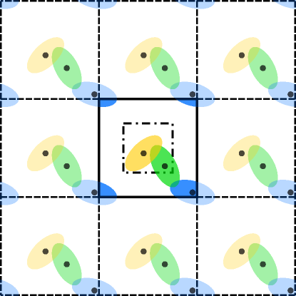
One obtains the n𝑛n-dimensional (unit) torus Tnsuperscript𝑇𝑛T^{n} by identifying opposite sides of the boundary of [1/2,1/2]nsuperscript1212𝑛[-1/2,1/2]^{n}. As in nsuperscript𝑛{\mathbb{R}}^{n} one can consider a translation invariant Poisson process of grains on the torus (with intensity measure ΛΛ\Lambda, grain distribution 𝐐𝐐\mathbf{Q} and intensity γ𝛾\gamma) and consider the resulting Boolean model ZTnsubscript𝑍superscript𝑇𝑛Z_{T^{n}}. The Boolean model on the torus Tnsuperscript𝑇𝑛T^{n} can be constructed in the following way from a random closed set in nsuperscript𝑛{\mathbb{R}}^{n} (see Fig. 1). We start with a homogeneous Poisson process in [1/2,1/2]nsuperscript1212𝑛[-1/2,1/2]^{n} and put around each point an independent copy of the typical grain. For each grain, we also place all translates by vectors vn𝑣superscript𝑛v\in\mathbb{Z}^{n} and take the union of all resulting grains. Finally, we restrict this random closed set to [1/2,1/2]nsuperscript1212𝑛[-1/2,1/2]^{n} and identify opposite boundaries. This setting is also denoted as periodic boundary conditions.
Refer to caption
Figure 1: The Boolean model with periodic boundary conditions: we consider grains with centers in [1/2,1/2]nsuperscript1212𝑛[-1/2,1/2]^{n} (square with solid line) and all their translations by nsuperscript𝑛\mathbb{Z}^{n} valued vectors (in squares with dashed lines). The Boolean model with periodic boundary conditions is obtained by taking the union of all the grains and restricting to the square with the solid line.

For a geometric functional ψ:n:𝜓superscript𝑛\psi:\mathcal{R}^{n}\to{\mathbb{R}} we can define ψ(ZTn)𝜓subscript𝑍superscript𝑇𝑛\psi(Z_{T^{n}}) in the following way. For a set KTn𝐾superscript𝑇𝑛K\subset T^{n} whose embedding Kn={xn:xK}subscript𝐾superscript𝑛conditional-set𝑥superscript𝑛𝑥𝐾K_{{\mathbb{R}}^{n}}=\{x\in{\mathbb{R}}^{n}:x\in K\} into nsuperscript𝑛{\mathbb{R}}^{n} is a convex body and is contained in (1/2,1/2)nsuperscript1212𝑛(-1/2,1/2)^{n} we put ψ(K)=ψ(Kn)𝜓𝐾𝜓subscript𝐾superscript𝑛\psi(K)=\psi(K_{{\mathbb{R}}^{n}}). By further requiring that ψ𝜓\psi is translation-invariant and additive on Tnsuperscript𝑇𝑛T^{n}, this gives us ψ(ZTn)𝜓subscript𝑍superscript𝑇𝑛\psi(Z_{T^{n}}).

By computing the Fock space representation of ψ(ZTn)𝜓subscript𝑍superscript𝑇𝑛\psi(Z_{T^{n}}) and ϕ(ZTn)italic-ϕsubscript𝑍superscript𝑇𝑛\phi(Z_{T^{n}}) for geometric functionals ψ,ϕ:n:𝜓italic-ϕsuperscript𝑛\psi,\phi:\mathcal{R}^{n}\to{\mathbb{R}} as in (HLS, , Section 3) for a Boolean model in nsuperscript𝑛{\mathbb{R}}^{n}, one obtains that

𝐜𝐨𝐯(ψ(ZTn),ϕ(ZTn))𝐜𝐨𝐯𝜓subscript𝑍superscript𝑇𝑛italic-ϕsubscript𝑍superscript𝑇𝑛\displaystyle\operatorname{\mathbf{cov}}(\psi(Z_{T^{n}}),\phi(Z_{T^{n}}))
=n=1γn!(𝐄ψ(ZTnK1Kn)ψ(K1Kn))absentsuperscriptsubscript𝑛1𝛾𝑛double-integral𝐄𝜓subscript𝑍superscript𝑇𝑛subscript𝐾1subscript𝐾𝑛𝜓subscript𝐾1subscript𝐾𝑛\displaystyle=\sum_{n=1}^{\infty}\frac{\gamma}{n!}\iint({\mathbf{E}}\psi(Z_{T^{n}}\cap K_{1}\cap\ldots\cap K_{n})-\psi(K_{1}\cap\ldots\cap K_{n}))
×(𝐄ϕ(ZTnK1Kn)ϕ(K1Kn))Λn1(d(K2,,Kn))𝐐(dK1).absent𝐄italic-ϕsubscript𝑍superscript𝑇𝑛subscript𝐾1subscript𝐾𝑛italic-ϕsubscript𝐾1subscript𝐾𝑛superscriptΛ𝑛1𝑑subscript𝐾2subscript𝐾𝑛𝐐𝑑subscript𝐾1\displaystyle\qquad\times({\mathbf{E}}\phi(Z_{T^{n}}\cap K_{1}\cap\ldots\cap K_{n})-\phi(K_{1}\cap\ldots\cap K_{n}))\,\Lambda^{n-1}(d(K_{2},\ldots,K_{n}))\,\mathbf{Q}(dK_{1}).

Now let us assume that the grain distribution 𝐐𝐐\mathbf{Q} is such that the typical grain Z0subscript𝑍0Z_{0} is almost surely contained in [1/4,1/4]nsuperscript1414𝑛[-1/4,1/4]^{n}, which is depicted by the dot-dash line in Fig. 1. In this case the intersection of two grains is always convex and the intersections on the right-hand side of the covariance formula are the same as for a Boolean model in nsuperscript𝑛{\mathbb{R}}^{n} with grain distribution 𝐐𝐐\mathbf{Q} and intensity γ𝛾\gamma. Thus, it follows from the above definition of ψ𝜓\psi and ϕitalic-ϕ\phi of a subset of the torus whose embedding into nsuperscript𝑛{\mathbb{R}}^{n} is a convex body and a subset of (1/2,1/2)nsuperscript1212𝑛(-1/2,1/2)^{n} and the additivity that

𝐜𝐨𝐯(ψ(ZTn),ϕ(ZTn))=ρ(ψ,ϕ).𝐜𝐨𝐯𝜓subscript𝑍superscript𝑇𝑛italic-ϕsubscript𝑍superscript𝑇𝑛𝜌superscript𝜓superscriptitalic-ϕ\operatorname{\mathbf{cov}}(\psi(Z_{T^{n}}),\phi(Z_{T^{n}}))=\rho(\psi^{*},\phi^{*}).

In other words, if the typical grain is sufficiently bounded, the exact covariances for the Boolean model on the torus coincide with the asymptotic covariances for the corresponding Boolean model in nsuperscript𝑛{\mathbb{R}}^{n}. This provides a way to compute estimates for the asymptotic covariances via simulations on the torus.

4 Central limit theorems

In this section we consider the asymptotic behaviour of the distributions of geometric functionals or of vectors of geometric functionals for growing observation window. Recall that a sequence of m𝑚m-dimensional random vectors (Yi)isubscriptsubscript𝑌𝑖𝑖(Y_{i})_{i\in\mathbb{N}} converges in distribution to an m𝑚m-dimensional random vector Y𝑌Y if

limi𝐏(Yix)=𝐏(Yx)subscript𝑖𝐏subscript𝑌𝑖𝑥𝐏𝑌𝑥\lim_{i\to\infty}{\mathbf{P}}(Y_{i}\leq x)={\mathbf{P}}(Y\leq x)

for all xm𝑥superscript𝑚x\in{\mathbb{R}}^{m} such that y𝐏(Yy)maps-to𝑦𝐏𝑌𝑦y\mapsto{\mathbf{P}}(Y\leq y) is continuous at x𝑥x. (Here the relation \leq is to be understood componentwise). In this case we write Yi𝑑Ysubscript𝑌𝑖𝑑𝑌Y_{i}\overset{d}{\longrightarrow}Y (as i𝑖i\to\infty). We are not only interested in the convergence in distribution but also in error bounds. In order to measure the distance between the distributions of two m𝑚m-dimensional random vectors Z1,Z2subscript𝑍1subscript𝑍2Z_{1},Z_{2}, we use the d3subscript𝑑3d_{3}-metric which is given by

d3(Z1,Z2)=suphm|𝐄h(Z1)𝐄h(Z2)|,subscript𝑑3subscript𝑍1subscript𝑍2subscriptsupremumsubscript𝑚𝐄subscript𝑍1𝐄subscript𝑍2d_{3}(Z_{1},Z_{2})=\sup_{h\in\mathcal{H}_{m}}|{\mathbf{E}}h(Z_{1})-{\mathbf{E}}h(Z_{2})|,

where msubscript𝑚\mathcal{H}_{m} is the set of all C3superscript𝐶3C^{3}-functions h:m:superscript𝑚h:{\mathbb{R}}^{m}\to{\mathbb{R}} such that the absolute values of the second and the third partial derivatives are bounded by one. For two random variables Z1,Z2subscript𝑍1subscript𝑍2Z_{1},Z_{2} we consider the Wasserstein distance

dW(Z1,Z2)=suphLip(1)|𝐄h(Z1)𝐄h(Z2)|,subscript𝑑𝑊subscript𝑍1subscript𝑍2subscriptsupremumLip1𝐄subscript𝑍1𝐄subscript𝑍2d_{W}(Z_{1},Z_{2})=\sup_{h\in\operatorname{Lip}(1)}|{\mathbf{E}}h(Z_{1})-{\mathbf{E}}h(Z_{2})|,

where Lip(1)Lip1\operatorname{Lip}(1) is the set of all functions h::h:{\mathbb{R}}\to{\mathbb{R}} whose Lipschitz constant is at most one. Note that convergence in the d3subscript𝑑3d_{3}-distance or in the Wasserstein distance implies convergence in distribution.

For the quantitative bounds we assume that there is a constant ε>0𝜀0\varepsilon>0 such that

𝐄Vi(Z0)3+ε<,i=0,,n.formulae-sequence𝐄subscript𝑉𝑖superscriptsubscript𝑍03𝜀𝑖0𝑛{\mathbf{E}}V_{i}(Z_{0})^{3+\varepsilon}<\infty,\quad i=0,\ldots,n. (39)

We begin with a multivariate central limit theorem for a vector of geometric functionals.

Theorem 4.1

Assume that (2) is satisfied, let Ψ:=(ψ1,,ψm)assignΨsubscript𝜓1subscript𝜓𝑚\Psi:=(\psi_{1},\ldots,\psi_{m}) for geometric functionals ψ1,,ψmsubscript𝜓1subscript𝜓𝑚\psi_{1},\ldots,\psi_{m}, and let NΣsubscript𝑁ΣN_{\Sigma} be an m𝑚m-dimensional centred Gaussian random vector with covariance matrix Σ=(σ(ψi,ψj))i,j=1,,mΣsubscript𝜎subscript𝜓𝑖subscript𝜓𝑗formulae-sequence𝑖𝑗1𝑚\Sigma=(\sigma(\psi_{i},\psi_{j}))_{i,j=1,\ldots,m}. Then

1Vn(W)(Ψ(ZW)𝐄Ψ(ZW))𝑑NΣ as r(W).1subscript𝑉𝑛𝑊Ψ𝑍𝑊𝐄Ψ𝑍𝑊𝑑subscript𝑁Σ as 𝑟𝑊\frac{1}{\sqrt{V_{n}(W)}}\big{(}\Psi(Z\cap W)-{\mathbf{E}}\Psi(Z\cap W)\big{)}\overset{d}{\longrightarrow}N_{\Sigma}\quad\text{ as }\quad r(W)\to\infty.

If (39) holds, there is a constant Cψ1,,ψmsubscript𝐶subscript𝜓1subscript𝜓𝑚C_{\psi_{1},\ldots,\psi_{m}} depending on ψ1,,ψmsubscript𝜓1subscript𝜓𝑚\psi_{1},\ldots,\psi_{m}, ΘΘ\Theta and ε𝜀\varepsilon such that

d3(1Vn(W)(Ψ(ZW)𝐄Ψ(ZW)),NΣ)Cψ1,ψmr(W)min{εn/2,1}subscript𝑑31subscript𝑉𝑛𝑊Ψ𝑍𝑊𝐄Ψ𝑍𝑊subscript𝑁Σsubscript𝐶subscript𝜓1subscript𝜓𝑚𝑟superscript𝑊𝜀𝑛21d_{3}\bigg{(}\frac{1}{\sqrt{V_{n}(W)}}\big{(}\Psi(Z\cap W)-{\mathbf{E}}\Psi(Z\cap W)\big{)},N_{\Sigma}\bigg{)}\leq\frac{C_{\psi_{1},\ldots\psi_{m}}}{r(W)^{\min\{\varepsilon n/2,1\}}}

for W𝒦n𝑊superscript𝒦𝑛W\in{\mathcal{K}}^{n} with r(W)1𝑟𝑊1r(W)\geq 1.

This result was proved in (HLS, , Theorem 9.1) by using the Stein-Malliavin method and a truncation argument.

As tensors can be interpreted as vectors, we can define convergence of tensor valued random elements and their d3subscript𝑑3d_{3}-distance via convergence and d3subscript𝑑3d_{3}-distance for random vectors. Since the components of Φm0,ssuperscriptsubscriptΦ𝑚0𝑠\Phi_{m}^{0,s} are geometric functionals, Theorem 4.1 can be applied to the translation invariant Minkowski tensors.

Corollary 2

Assume that (2) holds, let s𝑠s\in\mathbb{N} and m{0,,n1}𝑚0𝑛1m\in\{0,\ldots,n-1\} and let Nm0,ssubscriptsuperscript𝑁0𝑠𝑚N^{0,s}_{m} be a random element in 𝕋ssuperscript𝕋𝑠\mathbb{T}^{s} such that each component is a centred Gaussian random variable and

𝐜𝐨𝐯((N)i1,,is,(N)j1,,js)=σ((Φm0,s)i1,,is,(Φm0,s)j1,,js)𝐜𝐨𝐯subscript𝑁subscript𝑖1subscript𝑖𝑠subscript𝑁subscript𝑗1subscript𝑗𝑠𝜎subscriptsuperscriptsubscriptΦ𝑚0𝑠subscript𝑖1subscript𝑖𝑠subscriptsuperscriptsubscriptΦ𝑚0𝑠subscript𝑗1subscript𝑗𝑠\operatorname{\mathbf{cov}}((N)_{i_{1},\ldots,i_{s}},(N)_{j_{1},\ldots,j_{s}})=\sigma((\Phi_{m}^{0,s})_{i_{1},\ldots,i_{s}},(\Phi_{m}^{0,s})_{j_{1},\ldots,j_{s}})

for i1,,is,js,,js{1,,n}subscript𝑖1subscript𝑖𝑠subscript𝑗𝑠subscript𝑗𝑠1𝑛i_{1},\ldots,i_{s},j_{s},\ldots,j_{s}\in\{1,\ldots,n\}. Then

1Vn(W)(Φm0,s(ZW)𝐄Φm0,s(ZW))𝑑Nm0,s as r(W).1subscript𝑉𝑛𝑊superscriptsubscriptΦ𝑚0𝑠𝑍𝑊𝐄superscriptsubscriptΦ𝑚0𝑠𝑍𝑊𝑑subscriptsuperscript𝑁0𝑠𝑚 as 𝑟𝑊\frac{1}{\sqrt{V_{n}(W)}}(\Phi_{m}^{0,s}(Z\cap W)-{\mathbf{E}}\Phi_{m}^{0,s}(Z\cap W))\overset{d}{\longrightarrow}N^{0,s}_{m}\quad\text{ as }\quad r(W)\to\infty.

If (39) holds, there is a constant Cs,msubscript𝐶𝑠𝑚C_{s,m} depending on s𝑠s, m𝑚m, ΘΘ\Theta and ε𝜀\varepsilon such that

d3(1Vn(W)(Φm0,s(ZW)𝐄Φm0,s(ZW)),Nm0,s)Cs,mr(W)min{εn/2,1}subscript𝑑31subscript𝑉𝑛𝑊superscriptsubscriptΦ𝑚0𝑠𝑍𝑊𝐄superscriptsubscriptΦ𝑚0𝑠𝑍𝑊superscriptsubscript𝑁𝑚0𝑠subscript𝐶𝑠𝑚𝑟superscript𝑊𝜀𝑛21d_{3}\bigg{(}\frac{1}{\sqrt{V_{n}(W)}}(\Phi_{m}^{0,s}(Z\cap W)-{\mathbf{E}}\Phi_{m}^{0,s}(Z\cap W)),N_{m}^{0,s}\bigg{)}\leq\frac{C_{s,m}}{r(W)^{\min\{\varepsilon n/2,1\}}}

for W𝒦n𝑊superscript𝒦𝑛W\in{\mathcal{K}}^{n} with r(W)1𝑟𝑊1r(W)\geq 1.

In the multivariate case we assume translation invariance of the geometric functionals in order to ensure the existence of an asymptotic covariance matrix. In the univariate case this is not required since one can standardize be dividing by the standard deviation. For this reason, we can drop the assumption of translation invariance in the following univariate central limit theorem, which is taken from (HLS, , Theorem 9.3).

Theorem 4.2

Let (2) be satisfied, let ψ:n:𝜓superscript𝑛\psi:\mathcal{R}^{n}\to{\mathbb{R}} be measurable, additive and locally bounded, assume that there are constants r01subscript𝑟01r_{0}\geq 1 and σ0>0subscript𝜎00\sigma_{0}>0 such that

𝐯𝐚𝐫ψ(ZW)Vn(W)σ0𝐯𝐚𝐫𝜓𝑍𝑊subscript𝑉𝑛𝑊subscript𝜎0\frac{\operatorname{\mathbf{v}\mathbf{a}\mathbf{r}}\psi(Z\cap W)}{V_{n}(W)}\geq\sigma_{0}

for W𝒦n𝑊superscript𝒦𝑛W\in{\mathcal{K}}^{n} with r(W)r0𝑟𝑊subscript𝑟0r(W)\geq r_{0} and let N𝑁N be a standard Gaussian random variable. Then

ψ(ZW)𝐄ψ(ZW)𝐯𝐚𝐫ψ(ZW)𝑑N as r(W).𝜓𝑍𝑊𝐄𝜓𝑍𝑊𝐯𝐚𝐫𝜓𝑍𝑊𝑑𝑁 as 𝑟𝑊\frac{\psi(Z\cap W)-{\mathbf{E}}\psi(Z\cap W)}{\sqrt{\operatorname{\mathbf{v}\mathbf{a}\mathbf{r}}\psi(Z\cap W)}}\overset{d}{\longrightarrow}N\quad\text{ as }\quad r(W)\to\infty.

If, additionally, (39) is satisfied, there is a constant cψsubscript𝑐𝜓c_{\psi} depending on ψ𝜓\psi, ΘΘ\Theta, r0subscript𝑟0r_{0}, σ0subscript𝜎0\sigma_{0}, and ε𝜀\varepsilon such that

dW(ψ(ZW)𝐄ψ(ZW)𝐯𝐚𝐫ψ(ZW),N)cψVn(W)min{ε/2,1/2}subscript𝑑𝑊𝜓𝑍𝑊𝐄𝜓𝑍𝑊𝐯𝐚𝐫𝜓𝑍𝑊𝑁subscript𝑐𝜓subscript𝑉𝑛superscript𝑊𝜀212d_{W}\bigg{(}\frac{\psi(Z\cap W)-{\mathbf{E}}\psi(Z\cap W)}{\sqrt{\operatorname{\mathbf{v}\mathbf{a}\mathbf{r}}\psi(Z\cap W)}},N\bigg{)}\leq\frac{c_{\psi}}{V_{n}(W)^{\min\{\varepsilon/2,1/2\}}}

for W𝒦n𝑊superscript𝒦𝑛W\in{\mathcal{K}}^{n} with r(W)r0𝑟𝑊subscript𝑟0r(W)\geq r_{0}.

The results presented in this section generalize previous findings in BaryshnikovYukich ; Baddeley1980 ; Heinrich2005 ; HeinrichMolchanov1999 ; Mase1982 ; Molchanov1995 ; Penrose2007 , which only deal with volume, surface area or closely related functionals.

5 Boolean model of aligned rectangles

In this section we assume that n=2𝑛2n=2 and that the typical grain Z0subscript𝑍0Z_{0} is a deterministic rectangle of the form

K:=[a2e1,a2e1]+[b2e2,b2e2]=[a2,a2]×[b2,b2]assign𝐾𝑎2subscript𝑒1𝑎2subscript𝑒1𝑏2subscript𝑒2𝑏2subscript𝑒2𝑎2𝑎2𝑏2𝑏2K:=\Big{[}-\frac{a}{2}e_{1},\frac{a}{2}e_{1}\Big{]}+\Big{[}-\frac{b}{2}e_{2},\frac{b}{2}e_{2}\Big{]}=\Big{[}-\frac{a}{2},\frac{a}{2}\Big{]}\times\Big{[}-\frac{b}{2},\frac{b}{2}\Big{]}

for some fixed a,b>0𝑎𝑏0a,b>0, where e1:=(1,0)assignsubscript𝑒110e_{1}:=(1,0) and e2:=(0,1)assignsubscript𝑒201e_{2}:=(0,1). Then v2=absubscript𝑣2𝑎𝑏v_{2}=ab and v1=a+bsubscript𝑣1𝑎𝑏v_{1}=a+b.

Refer to caption
Refer to caption
Refer to caption
Refer to caption
Refer to caption
Refer to caption
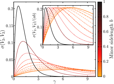
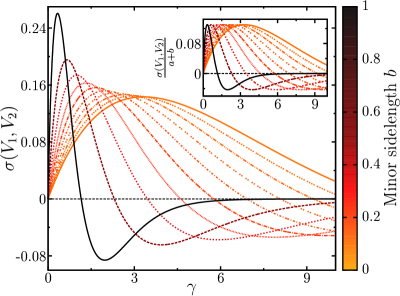
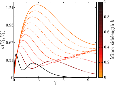
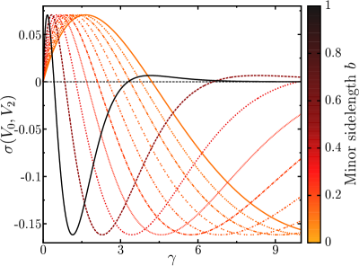
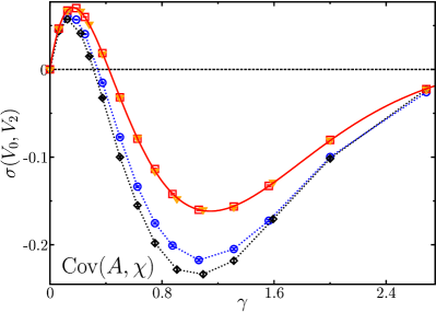
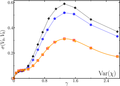
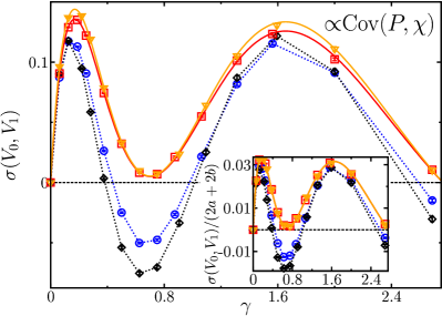
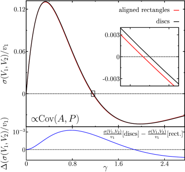
Figure 2: Asymptotic covariances σ(Vi,Vj)𝜎subscript𝑉𝑖subscript𝑉𝑗\sigma(V_{i},V_{j}) as a function of the intensity γ𝛾\gamma for Boolean models of aligned rectangles with varying aspect ratio b/a𝑏𝑎b/a; we choose a=1𝑎1a=1, hence b(0,1]𝑏01b\in(0,1]; see Eqs. (42), (52), (54), (66), (71), and (76). The insets show covariances that are rescaled by suitable functions of the side lengths a𝑎a and b𝑏b of a single rectangle so that they only depend on γv2𝛾subscript𝑣2\gamma v_{2} but not on the aspect ratio, which also holds for σ(V0,V2)𝜎subscript𝑉0subscript𝑉2\sigma(V_{0},V_{2}) in (d) without rescaling.

For any x=(x1,x2)2𝑥subscript𝑥1subscript𝑥2superscript2x=(x_{1},x_{2})\in{\mathbb{R}}^{2} we have

C2(x)=V2(K(K+x))=𝟏{|x1|a,|x2|b}(a|x1|)(b|x2|).subscript𝐶2𝑥subscript𝑉2𝐾𝐾𝑥1formulae-sequencesubscript𝑥1𝑎subscript𝑥2𝑏𝑎subscript𝑥1𝑏subscript𝑥2C_{2}(x)=V_{2}(K\cap(K+x))={\mathbf{1}}\{|x_{1}|\leq a,|x_{2}|\leq b\}(a-|x_{1}|)(b-|x_{2}|).

A change of variables and a symmetry argument imply that

(eγC2(x)1)𝑑x=4v2H(γv2),superscript𝑒𝛾subscript𝐶2𝑥1differential-d𝑥4subscript𝑣2𝐻𝛾subscript𝑣2\displaystyle\int\big{(}e^{\gamma C_{2}(x)}-1\big{)}\,dx=4v_{2}H(\gamma v_{2}), (40)

where the function H:[0,)[0,):𝐻00H:[0,\infty)\to[0,\infty) is defined by

H(r):=0101(erst1)𝑑s𝑑t=k=1rkk!(k+1)2,r0.formulae-sequenceassign𝐻𝑟subscriptsuperscript10subscriptsuperscript10superscript𝑒𝑟𝑠𝑡1differential-d𝑠differential-d𝑡subscriptsuperscript𝑘1superscript𝑟𝑘𝑘superscript𝑘12𝑟0\displaystyle H(r):=\int^{1}_{0}\int^{1}_{0}\big{(}e^{rst}-1\big{)}\,ds\,dt=\sum^{\infty}_{k=1}\frac{r^{k}}{k!(k+1)^{2}},\quad r\geq 0. (41)

Hence we obtain from Theorem 3.2 that

σ(V2,V2)=4(1p)2v2H(γv2),𝜎subscript𝑉2subscript𝑉24superscript1𝑝2subscript𝑣2𝐻𝛾subscript𝑣2\displaystyle\sigma(V_{2},V_{2})=4(1-p)^{2}v_{2}H(\gamma v_{2}), (42)

where we recall that p=1eγv2𝑝1superscript𝑒𝛾subscript𝑣2p=1-e^{-\gamma v_{2}}. The variance is visualized in Fig. 2.

At this stage it is convenient to complement the definition (41) with the following easy to check formulae:

0101ersts𝑑s𝑑tsubscriptsuperscript10subscriptsuperscript10superscript𝑒𝑟𝑠𝑡𝑠differential-d𝑠differential-d𝑡\displaystyle\int^{1}_{0}\int^{1}_{0}e^{rst}s\,ds\,dt =1r2er1r21r,absent1superscript𝑟2superscript𝑒𝑟1superscript𝑟21𝑟\displaystyle=\frac{1}{r^{2}}e^{r}-\frac{1}{r^{2}}-\frac{1}{r},\allowdisplaybreaks (43)
0101ersts2𝑑s𝑑tsubscriptsuperscript10subscriptsuperscript10superscript𝑒𝑟𝑠𝑡superscript𝑠2differential-d𝑠differential-d𝑡\displaystyle\int^{1}_{0}\int^{1}_{0}e^{rst}s^{2}\,ds\,dt =1r2er1r3er+1r312r,absent1superscript𝑟2superscript𝑒𝑟1superscript𝑟3superscript𝑒𝑟1superscript𝑟312𝑟\displaystyle=\frac{1}{r^{2}}e^{r}-\frac{1}{r^{3}}e^{r}+\frac{1}{r^{3}}-\frac{1}{2r},\allowdisplaybreaks (44)
0101erstst𝑑s𝑑tsubscriptsuperscript10subscriptsuperscript10superscript𝑒𝑟𝑠𝑡𝑠𝑡differential-d𝑠differential-d𝑡\displaystyle\int^{1}_{0}\int^{1}_{0}e^{rst}st\,ds\,dt =1r2er1r21rH(r)1r.absent1superscript𝑟2superscript𝑒𝑟1superscript𝑟21𝑟𝐻𝑟1𝑟\displaystyle=\frac{1}{r^{2}}e^{r}-\frac{1}{r^{2}}-\frac{1}{r}H(r)-\frac{1}{r}. (45)

A consequence is

0101erst(st+s2)𝑑s𝑑tsubscriptsuperscript10subscriptsuperscript10superscript𝑒𝑟𝑠𝑡𝑠𝑡superscript𝑠2differential-d𝑠differential-d𝑡\displaystyle\int^{1}_{0}\int^{1}_{0}e^{rst}(st+s^{2})\,ds\,dt =2r2er1r3er+1r31r232r1rH(r).absent2superscript𝑟2superscript𝑒𝑟1superscript𝑟3superscript𝑒𝑟1superscript𝑟31superscript𝑟232𝑟1𝑟𝐻𝑟\displaystyle=\frac{2}{r^{2}}e^{r}-\frac{1}{r^{3}}e^{r}+\frac{1}{r^{3}}-\frac{1}{r^{2}}-\frac{3}{2r}-\frac{1}{r}H(r). (46)

Now we use Theorem 3.2 (for n=2𝑛2n=2 and g1𝑔1g\equiv 1) to compute σ(V1,V2)𝜎subscript𝑉1subscript𝑉2\sigma(V_{1},V_{2}). For any measurable and even functions f:2[0,):𝑓superscript20f:{\mathbb{R}}^{2}\to[0,\infty) and f~:𝕊1[0,):~𝑓superscript𝕊10\tilde{f}:{\mathbb{S}}^{1}\to[0,\infty) we have

f(yz)f~(u)N1,2(d(y,u,z))=a1++a1+a2++a2,𝑓𝑦𝑧~𝑓𝑢subscript𝑁12𝑑𝑦𝑢𝑧subscriptsuperscript𝑎1subscriptsuperscript𝑎1subscriptsuperscript𝑎2subscriptsuperscript𝑎2\displaystyle\int f(y-z)\tilde{f}(u)\,N_{1,2}(d(y,u,z))=a^{+}_{1}+a^{-}_{1}+a^{+}_{2}+a^{-}_{2},

where

ai±:=12𝟏{yAi±,zK}f(yz)f~(ei)1(dy)𝑑z,i{1,2}formulae-sequenceassignsubscriptsuperscript𝑎plus-or-minus𝑖12double-integral1formulae-sequence𝑦subscriptsuperscript𝐴plus-or-minus𝑖𝑧𝐾𝑓𝑦𝑧~𝑓subscript𝑒𝑖superscript1𝑑𝑦differential-d𝑧𝑖12\displaystyle a^{\pm}_{i}:=\frac{1}{2}\iint{\mathbf{1}}\{y\in A^{\pm}_{i},z\in K\}f(y-z)\tilde{f}(e_{i})\,{\mathcal{H}}^{1}(dy)\,dz,\quad i\in\{1,2\}

and A1±:={(x1,x2)K:x1=±a/2}assignsubscriptsuperscript𝐴plus-or-minus1conditional-setsubscript𝑥1subscript𝑥2𝐾subscript𝑥1plus-or-minus𝑎2A^{\pm}_{1}:=\{(x_{1},x_{2})\in K:x_{1}=\pm a/2\}, A2±:={(x1,x2)K:x2=±b/2}assignsubscriptsuperscript𝐴plus-or-minus2conditional-setsubscript𝑥1subscript𝑥2𝐾subscript𝑥2plus-or-minus𝑏2A^{\pm}_{2}:=\{(x_{1},x_{2})\in K:x_{2}=\pm b/2\}. By Fubini and a change of variables

a1±=f~(e1)2𝟏{yA1±,y+zK}f(z)1(dy)𝑑z.subscriptsuperscript𝑎plus-or-minus1~𝑓subscript𝑒12double-integral1formulae-sequence𝑦subscriptsuperscript𝐴plus-or-minus1𝑦𝑧𝐾𝑓𝑧superscript1𝑑𝑦differential-d𝑧\displaystyle a^{\pm}_{1}=\frac{\tilde{f}(e_{1})}{2}\iint{\mathbf{1}}\{y\in A^{\pm}_{1},y+z\in K\}f(z)\,{\mathcal{H}}^{1}(dy)\,dz. (47)

For any z=(z1,z2)K𝑧subscript𝑧1subscript𝑧2𝐾z=(z_{1},z_{2})\in K with az10𝑎subscript𝑧10-a\leq z_{1}\leq 0 and z20subscript𝑧20z_{2}\geq 0 we have

𝟏{yA1,y+zK}1(dy)=1([b/2,b/2z2])=bz2=b|z2|.1formulae-sequence𝑦subscript𝐴1𝑦𝑧𝐾superscript1𝑑𝑦superscript1𝑏2𝑏2subscript𝑧2𝑏subscript𝑧2𝑏subscript𝑧2\displaystyle\int{\mathbf{1}}\{y\in A_{1},y+z\in K\}\,{\mathcal{H}}^{1}(dy)={\mathcal{H}}^{1}([-b/2,b/2-z_{2}])=b-z_{2}=b-|z_{2}|.

For az10𝑎subscript𝑧10-a\leq z_{1}\leq 0 and z20subscript𝑧20z_{2}\leq 0 this integral takes the same value. Since the set of all z𝑧z with z1[a,0]subscript𝑧1𝑎0z_{1}\notin[-a,0] or |z2|>bsubscript𝑧2𝑏|z_{2}|>b does not contribute to a+superscript𝑎a^{+} while the set of all z𝑧z with z1[0,a]subscript𝑧10𝑎z_{1}\notin[0,a] or |z2|>bsubscript𝑧2𝑏|z_{2}|>b does not contribute to asuperscript𝑎a^{-} it follows that

a1++a1=subscriptsuperscript𝑎1subscriptsuperscript𝑎1absent\displaystyle a^{+}_{1}+a^{-}_{1}=\; f~(e1)2𝟏{|z1|a,|z2|b}f(z1,z2)(b|z2|)d(z1,z2).~𝑓subscript𝑒121formulae-sequencesubscript𝑧1𝑎subscript𝑧2𝑏𝑓subscript𝑧1subscript𝑧2𝑏subscript𝑧2𝑑subscript𝑧1subscript𝑧2\displaystyle\frac{\tilde{f}(e_{1})}{2}\int{\mathbf{1}}\{|z_{1}|\leq a,|z_{2}|\leq b\}f(z_{1},z_{2})(b-|z_{2}|)\,d(z_{1},z_{2}). (48)

Using a similar result for b1++b1subscriptsuperscript𝑏1subscriptsuperscript𝑏1b^{+}_{1}+b^{-}_{1} gives

f(yz)f~(u)𝑓𝑦𝑧~𝑓𝑢\displaystyle\int f(y-z)\tilde{f}(u) N1,2(d(y,u,z))subscript𝑁12𝑑𝑦𝑢𝑧\displaystyle\,N_{1,2}(d(y,u,z))
=\displaystyle=\; f~(e1)2𝟏{|z1|a,|z2|b}f(z1,z2)(b|z2|)d(z1,z2)~𝑓subscript𝑒121formulae-sequencesubscript𝑧1𝑎subscript𝑧2𝑏𝑓subscript𝑧1subscript𝑧2𝑏subscript𝑧2𝑑subscript𝑧1subscript𝑧2\displaystyle\frac{\tilde{f}(e_{1})}{2}\int{\mathbf{1}}\{|z_{1}|\leq a,|z_{2}|\leq b\}f(z_{1},z_{2})(b-|z_{2}|)\,d(z_{1},z_{2})
+f~(e2)2𝟏{|z1|a,|z2|b}f(z1,z2)(a|z1|)d(z1,z2).~𝑓subscript𝑒221formulae-sequencesubscript𝑧1𝑎subscript𝑧2𝑏𝑓subscript𝑧1subscript𝑧2𝑎subscript𝑧1𝑑subscript𝑧1subscript𝑧2\displaystyle+\frac{\tilde{f}(e_{2})}{2}\int{\mathbf{1}}\{|z_{1}|\leq a,|z_{2}|\leq b\}f(z_{1},z_{2})(a-|z_{1}|)\,d(z_{1},z_{2}). (49)

Inserting here f(z):=eγC2(z)assign𝑓𝑧superscript𝑒𝛾subscript𝐶2𝑧f(z):=e^{\gamma C_{2}(z)} and using a change of variables gives

\displaystyle\int eγC2(yz)f~(u)N1,2(d(y,u,z))superscript𝑒𝛾subscript𝐶2𝑦𝑧~𝑓𝑢subscript𝑁12𝑑𝑦𝑢𝑧\displaystyle e^{\gamma C_{2}(y-z)}\tilde{f}(u)\,N_{1,2}(d(y,u,z))
=2ab2f~(e1)0101eγaby1y2y2𝑑y1𝑑y2+2a2bf~(e2)0101eγaby1y2y1𝑑y1𝑑y2.absent2𝑎superscript𝑏2~𝑓subscript𝑒1subscriptsuperscript10subscriptsuperscript10superscript𝑒𝛾𝑎𝑏subscript𝑦1subscript𝑦2subscript𝑦2differential-dsubscript𝑦1differential-dsubscript𝑦22superscript𝑎2𝑏~𝑓subscript𝑒2subscriptsuperscript10subscriptsuperscript10superscript𝑒𝛾𝑎𝑏subscript𝑦1subscript𝑦2subscript𝑦1differential-dsubscript𝑦1differential-dsubscript𝑦2\displaystyle=2ab^{2}\tilde{f}(e_{1})\int^{1}_{0}\int^{1}_{0}e^{\gamma aby_{1}y_{2}}y_{2}\,dy_{1}\,dy_{2}+2a^{2}b\tilde{f}(e_{2})\int^{1}_{0}\int^{1}_{0}e^{\gamma aby_{1}y_{2}}y_{1}\,dy_{1}\,dy_{2}.

From (43) we obtain that

\displaystyle\int eγC2(yz)f~(u)N1,2(d(y,u,z))superscript𝑒𝛾subscript𝐶2𝑦𝑧~𝑓𝑢subscript𝑁12𝑑𝑦𝑢𝑧\displaystyle e^{\gamma C_{2}(y-z)}\tilde{f}(u)\,N_{1,2}(d(y,u,z))
=f~(e1)(2γ2aeγab2γ2a2bγ)+f~(e2)(2γ2beγab2γ2b2aγ).absent~𝑓subscript𝑒12superscript𝛾2𝑎superscript𝑒𝛾𝑎𝑏2superscript𝛾2𝑎2𝑏𝛾~𝑓subscript𝑒22superscript𝛾2𝑏superscript𝑒𝛾𝑎𝑏2superscript𝛾2𝑏2𝑎𝛾\displaystyle=\tilde{f}(e_{1})\bigg{(}\frac{2}{\gamma^{2}a}e^{\gamma ab}-\frac{2}{\gamma^{2}a}-\frac{2b}{\gamma}\bigg{)}+\tilde{f}(e_{2})\bigg{(}\frac{2}{\gamma^{2}b}e^{\gamma ab}-\frac{2}{\gamma^{2}b}-\frac{2a}{\gamma}\bigg{)}. (50)

In the case f~(e1)=f~(e2)=1~𝑓subscript𝑒1~𝑓subscript𝑒21\tilde{f}(e_{1})=\tilde{f}(e_{2})=1 this yields

eγC2(xy)N1,2(d(x,u,y))=2v1(1γ2v2eγv21γ2v21γ).superscript𝑒𝛾subscript𝐶2𝑥𝑦subscript𝑁12𝑑𝑥𝑢𝑦2subscript𝑣11superscript𝛾2subscript𝑣2superscript𝑒𝛾subscript𝑣21superscript𝛾2subscript𝑣21𝛾\displaystyle\int e^{\gamma C_{2}(x-y)}\,N_{1,2}(d(x,u,y))=2v_{1}\bigg{(}\frac{1}{\gamma^{2}v_{2}}e^{\gamma v_{2}}-\frac{1}{\gamma^{2}v_{2}}-\frac{1}{\gamma}\bigg{)}. (51)

Inserting this result together with (40) into the formula of Theorem 3.2 yields

σ(V1,V2)=2(1p)2v1[1γv2(eγv21)12γv2H(γv2)],𝜎subscript𝑉1subscript𝑉22superscript1𝑝2subscript𝑣1delimited-[]1𝛾subscript𝑣2superscript𝑒𝛾subscript𝑣2112𝛾subscript𝑣2𝐻𝛾subscript𝑣2\displaystyle\sigma(V_{1},V_{2})=2(1-p)^{2}v_{1}\left[\frac{1}{\gamma v_{2}}(e^{\gamma v_{2}}-1)-1-2\gamma v_{2}H(\gamma v_{2})\right], (52)

which is visualized in Fig. 2.

Next we use (3.4) to compute σ(V0,V2)𝜎subscript𝑉0subscript𝑉2\sigma(V_{0},V_{2}), starting with the observation

h(K,e1)=h(K,e1)=a2,h(K,e2)=h(K,e2)=b2.formulae-sequence𝐾subscript𝑒1𝐾subscript𝑒1𝑎2𝐾subscript𝑒2𝐾subscript𝑒2𝑏2h(K,-e_{1})=h(K,e_{1})=\frac{a}{2},\qquad h(K,-e_{2})=h(K,e_{2})=\frac{b}{2}.

Therefore we obtain from (5)

h¯(u)eγC2(yz)N1,2(d(y,u,z))=2γ2eγv22γ22v2γ.¯𝑢superscript𝑒𝛾subscript𝐶2𝑦𝑧subscript𝑁12𝑑𝑦𝑢𝑧2superscript𝛾2superscript𝑒𝛾subscript𝑣22superscript𝛾22subscript𝑣2𝛾\displaystyle\int\bar{h}(u)e^{\gamma C_{2}(y-z)}\,N_{1,2}(d(y,u,z))=\frac{2}{\gamma^{2}}e^{\gamma v_{2}}-\frac{2}{\gamma^{2}}-\frac{2v_{2}}{\gamma}. (53)

To evaluate

v1,1=h(K,u)Ψ1(K;du)subscript𝑣11𝐾𝑢subscriptΨ1𝐾𝑑𝑢v_{1,1}=\int h(K,u)\,\Psi_{1}(K;du)

we split the integration according to u{e1,e1,e2,e2}𝑢subscript𝑒1subscript𝑒1subscript𝑒2subscript𝑒2u\in\{-e_{1},e_{1},-e_{2},e_{2}\}. As all four integrals yield the same value ab/4𝑎𝑏4ab/4, we get v1,1=v2subscript𝑣11subscript𝑣2v_{1,1}=v_{2}. Summarizing, we obtain from (3.4)

σ(V0,V2)=𝜎subscript𝑉0subscript𝑉2absent\displaystyle\sigma(V_{0},V_{2})=\; p(1p)4(1p)2γv2(11γv2)H(γv2)𝑝1𝑝4superscript1𝑝2𝛾subscript𝑣211𝛾subscript𝑣2𝐻𝛾subscript𝑣2\displaystyle p(1-p)-4(1-p)^{2}\gamma v_{2}(1-1\gamma v_{2})H(\gamma v_{2})
4(1p)2((1p)11γv2),4superscript1𝑝2superscript1𝑝11𝛾subscript𝑣2\displaystyle-4(1-p)^{2}\big{(}(1-p)^{-1}-1-\gamma v_{2}\big{)},

that is

σ(V0,V2)=(1p)[2(1p)γv23p(1p)γv2(42γv2)H(γv2)].𝜎subscript𝑉0subscript𝑉21𝑝delimited-[]21𝑝𝛾subscript𝑣23𝑝1𝑝𝛾subscript𝑣242𝛾subscript𝑣2𝐻𝛾subscript𝑣2\displaystyle\sigma(V_{0},V_{2})=(1-p)\left[2(1-p)\gamma v_{2}-3p-(1-p)\gamma v_{2}(4-2\gamma v_{2})H(\gamma v_{2})\right]. (54)

Figure 2 visualizes this asymptotic covariance.

Next we turn to σ(V1,V1)𝜎subscript𝑉1subscript𝑉1\sigma(V_{1},V_{1}) as given by (3.1) for n=2𝑛2n=2. Some of our calculations will also be required to compute σ(V0,V1)𝜎subscript𝑉0subscript𝑉1\sigma(V_{0},V_{1}) and σ(V0,V0)𝜎subscript𝑉0subscript𝑉0\sigma(V_{0},V_{0}). We have

C1(x;h¯)=subscript𝐶1𝑥¯absent\displaystyle C_{1}(x;\bar{h})=\; a4𝟏{yxK0,yA1+A1}1(dy)𝑎41formulae-sequence𝑦𝑥superscript𝐾0𝑦subscriptsuperscript𝐴1subscriptsuperscript𝐴1superscript1𝑑𝑦\displaystyle\frac{a}{4}\int{\mathbf{1}}\{y-x\in K^{0},y\in A^{+}_{1}\cup A^{-}_{1}\}\,{\mathcal{H}}^{1}(dy) (55)
+b4𝟏{yxK0,yA2+A2}1(dy)𝑏41formulae-sequence𝑦𝑥superscript𝐾0𝑦subscriptsuperscript𝐴2subscriptsuperscript𝐴2superscript1𝑑𝑦\displaystyle+\frac{b}{4}\int{\mathbf{1}}\{y-x\in K^{0},y\in A^{+}_{2}\cup A^{-}_{2}\}\,{\mathcal{H}}^{1}(dy) (56)

and a straightforward calculation (left to the reader) yields

C1(x;h¯)=𝟏{|x1|a,|x2|b}(a4(b|x2|)+b4(a|x1|))subscript𝐶1𝑥¯1formulae-sequencesubscript𝑥1𝑎subscript𝑥2𝑏𝑎4𝑏subscript𝑥2𝑏4𝑎subscript𝑥1\displaystyle C_{1}(x;\bar{h})={\mathbf{1}}\{|x_{1}|\leq a,|x_{2}|\leq b\}\Big{(}\frac{a}{4}(b-|x_{2}|)+\frac{b}{4}(a-|x_{1}|)\Big{)} (57)

as well as

C1(x)=12𝟏{|x1|a,|x2|b}((a|x1|)+(b|x2|)).subscript𝐶1𝑥121formulae-sequencesubscript𝑥1𝑎subscript𝑥2𝑏𝑎subscript𝑥1𝑏subscript𝑥2\displaystyle C_{1}(x)=\frac{1}{2}{\mathbf{1}}\{|x_{1}|\leq a,|x_{2}|\leq b\}((a-|x_{1}|)+(b-|x_{2}|)). (58)

From C1(x;h¯)=C1(x;h¯)subscript𝐶1𝑥¯subscript𝐶1𝑥¯C_{1}(x;\bar{h})=C_{1}(-x;\bar{h}) (see (57)) and (5) (with f(x):=eγC2(x)assign𝑓𝑥superscript𝑒𝛾subscript𝐶2𝑥f(x):=e^{\gamma C_{2}(x)} and f~1~𝑓1\tilde{f}\equiv 1) it follows that

eγC2(yz)C1(yz;h¯)N1,2(d(z,u,y))=J1+J2,superscript𝑒𝛾subscript𝐶2𝑦𝑧subscript𝐶1𝑦𝑧¯subscript𝑁12𝑑𝑧𝑢𝑦subscript𝐽1subscript𝐽2\displaystyle\int e^{\gamma C_{2}(y-z)}C_{1}(y-z;\bar{h})\,N_{1,2}(d(z,u,y))=J_{1}+J_{2},

where

J1:=assignsubscript𝐽1absent\displaystyle J_{1}:=\; a8[a,a]×[b,b]eγ(a|z1|)(b|z2|)((a|z1|)+(b|z2|))(b|z2|)d(z1,z2)𝑎8subscript𝑎𝑎𝑏𝑏superscript𝑒𝛾𝑎subscript𝑧1𝑏subscript𝑧2𝑎subscript𝑧1𝑏subscript𝑧2𝑏subscript𝑧2𝑑subscript𝑧1subscript𝑧2\displaystyle\frac{a}{8}\int_{[-a,a]\times[-b,b]}e^{\gamma(a-|z_{1}|)(b-|z_{2}|)}((a-|z_{1}|)+(b-|z_{2}|))(b-|z_{2}|)\,d(z_{1},z_{2})

and J2subscript𝐽2J_{2} is defined similarly. We have

J1subscript𝐽1\displaystyle J_{1} =a2𝟏{0z1a,0z2b}eγz1z2(z1+z2)z2d(z1,z2)\displaystyle=\frac{a}{2}\int{\mathbf{1}}\{0\leq z_{1}\leq a,0\leq z_{2}\leq b\}e^{\gamma z_{1}z_{2}}(z_{1}+z_{2})z_{2}\,d(z_{1},z_{2})
=a2b220101eγabst(as+bt)t𝑑s𝑑tabsentsuperscript𝑎2superscript𝑏22subscriptsuperscript10subscriptsuperscript10superscript𝑒𝛾𝑎𝑏𝑠𝑡𝑎𝑠𝑏𝑡𝑡differential-d𝑠differential-d𝑡\displaystyle=\frac{a^{2}b^{2}}{2}\int^{1}_{0}\int^{1}_{0}e^{\gamma abst}(as+bt)t\,ds\,dt
=a3b220101eγabstst𝑑s𝑑t+a2b320101eγabstt2𝑑s𝑑t.absentsuperscript𝑎3superscript𝑏22subscriptsuperscript10subscriptsuperscript10superscript𝑒𝛾𝑎𝑏𝑠𝑡𝑠𝑡differential-d𝑠differential-d𝑡superscript𝑎2superscript𝑏32subscriptsuperscript10subscriptsuperscript10superscript𝑒𝛾𝑎𝑏𝑠𝑡superscript𝑡2differential-d𝑠differential-d𝑡\displaystyle=\frac{a^{3}b^{2}}{2}\int^{1}_{0}\int^{1}_{0}e^{\gamma abst}st\,ds\,dt+\frac{a^{2}b^{3}}{2}\int^{1}_{0}\int^{1}_{0}e^{\gamma abst}t^{2}\,ds\,dt.

Together with the analogous formula for J2subscript𝐽2J_{2} this yields

eγC2(yz)C1(yz;h¯)N1,2(d(z,u,y))=v1v2220101eγv2st(st+t2)𝑑s𝑑t.superscript𝑒𝛾subscript𝐶2𝑦𝑧subscript𝐶1𝑦𝑧¯subscript𝑁12𝑑𝑧𝑢𝑦subscript𝑣1subscriptsuperscript𝑣222subscriptsuperscript10subscriptsuperscript10superscript𝑒𝛾subscript𝑣2𝑠𝑡𝑠𝑡superscript𝑡2differential-d𝑠differential-d𝑡\displaystyle\int e^{\gamma C_{2}(y-z)}C_{1}(y-z;\bar{h})\,N_{1,2}(d(z,u,y))=\frac{v_{1}v^{2}_{2}}{2}\int^{1}_{0}\int^{1}_{0}e^{\gamma v_{2}st}(st+t^{2})\,ds\,dt.

Now we can use (46) with r=γv2𝑟𝛾subscript𝑣2r=\gamma v_{2} to obtain

eγC2(yz)superscript𝑒𝛾subscript𝐶2𝑦𝑧\displaystyle\int e^{\gamma C_{2}(y-z)} C1(yz;h¯)N1,2(d(z,u,y))subscript𝐶1𝑦𝑧¯subscript𝑁12𝑑𝑧𝑢𝑦\displaystyle C_{1}(y-z;\bar{h})\,N_{1,2}(d(z,u,y))
=v1γ2eγv2v12γ3v2eγv2+v12γ3v2v12γ23v1v24γv1v22γH(γv2).absentsubscript𝑣1superscript𝛾2superscript𝑒𝛾subscript𝑣2subscript𝑣12superscript𝛾3subscript𝑣2superscript𝑒𝛾subscript𝑣2subscript𝑣12superscript𝛾3subscript𝑣2subscript𝑣12superscript𝛾23subscript𝑣1subscript𝑣24𝛾subscript𝑣1subscript𝑣22𝛾𝐻𝛾subscript𝑣2\displaystyle=\frac{v_{1}}{\gamma^{2}}e^{\gamma v_{2}}-\frac{v_{1}}{2\gamma^{3}v_{2}}e^{\gamma v_{2}}+\frac{v_{1}}{2\gamma^{3}v_{2}}-\frac{v_{1}}{2\gamma^{2}}-\frac{3v_{1}v_{2}}{4\gamma}-\frac{v_{1}v_{2}}{2\gamma}H(\gamma v_{2}). (59)

Similarly,

eγC2(yz)superscript𝑒𝛾subscript𝐶2𝑦𝑧\displaystyle\int e^{\gamma C_{2}(y-z)} C1(yz)N1,2(d(z,u,y))subscript𝐶1𝑦𝑧subscript𝑁12𝑑𝑧𝑢𝑦\displaystyle C_{1}(y-z)\,N_{1,2}(d(z,u,y))
=\displaystyle=\; 𝟏{0z1a,0z2b}eγz1z2(z1+z2)2d(z1,z2)\displaystyle\int{\mathbf{1}}\{0\leq z_{1}\leq a,0\leq z_{2}\leq b\}e^{\gamma z_{1}z_{2}}(z_{1}+z_{2})^{2}\,d(z_{1},z_{2})
=\displaystyle=\; ab0101eγabst(as+bt)2𝑑s𝑑t𝑎𝑏subscriptsuperscript10subscriptsuperscript10superscript𝑒𝛾𝑎𝑏𝑠𝑡superscript𝑎𝑠𝑏𝑡2differential-d𝑠differential-d𝑡\displaystyle ab\int^{1}_{0}\int^{1}_{0}e^{\gamma abst}(as+bt)^{2}\,ds\,dt
=\displaystyle=\; ab(a2+b2)0101eγabsts2𝑑s𝑑t+2a2b20101eγabstst𝑑s𝑑t.𝑎𝑏superscript𝑎2superscript𝑏2subscriptsuperscript10subscriptsuperscript10superscript𝑒𝛾𝑎𝑏𝑠𝑡superscript𝑠2differential-d𝑠differential-d𝑡2superscript𝑎2superscript𝑏2subscriptsuperscript10subscriptsuperscript10superscript𝑒𝛾𝑎𝑏𝑠𝑡𝑠𝑡differential-d𝑠differential-d𝑡\displaystyle ab(a^{2}+b^{2})\int^{1}_{0}\int^{1}_{0}e^{\gamma abst}s^{2}\,ds\,dt+2a^{2}b^{2}\int^{1}_{0}\int^{1}_{0}e^{\gamma abst}st\,ds\,dt.

It follows from (44) and (45) that the latter sum equals

ab𝑎𝑏\displaystyle ab (a2+b2)(1γ2a2b2eγv21γ3a3b3eγv2+1γ3a3b312γab)superscript𝑎2superscript𝑏21superscript𝛾2superscript𝑎2superscript𝑏2superscript𝑒𝛾subscript𝑣21superscript𝛾3superscript𝑎3superscript𝑏3superscript𝑒𝛾subscript𝑣21superscript𝛾3superscript𝑎3superscript𝑏312𝛾𝑎𝑏\displaystyle(a^{2}+b^{2})\Big{(}\frac{1}{\gamma^{2}a^{2}b^{2}}e^{\gamma v_{2}}-\frac{1}{\gamma^{3}a^{3}b^{3}}e^{\gamma v_{2}}+\frac{1}{\gamma^{3}a^{3}b^{3}}-\frac{1}{2\gamma ab}\Big{)}
+2a2b2(1γ2a2b2eγab1γ2a2b21γabH(γab)1γab).2superscript𝑎2superscript𝑏21superscript𝛾2superscript𝑎2superscript𝑏2superscript𝑒𝛾𝑎𝑏1superscript𝛾2superscript𝑎2superscript𝑏21𝛾𝑎𝑏𝐻𝛾𝑎𝑏1𝛾𝑎𝑏\displaystyle+2a^{2}b^{2}\Big{(}\frac{1}{\gamma^{2}a^{2}b^{2}}e^{\gamma ab}-\frac{1}{\gamma^{2}a^{2}b^{2}}-\frac{1}{\gamma ab}H(\gamma ab)-\frac{1}{\gamma ab}\Big{)}.

Therefore

γ2superscript𝛾2\displaystyle\gamma^{2} eγC2(yz)C1(yz)N1,2(d(z,u,y))superscript𝑒𝛾subscript𝐶2𝑦𝑧subscript𝐶1𝑦𝑧subscript𝑁12𝑑𝑧𝑢𝑦\displaystyle\int e^{\gamma C_{2}(y-z)}C_{1}(y-z)\,N_{1,2}(d(z,u,y))
=(a2+b2)(1v2eγv21γv22eγv2+1γv22γ2)+2eγv222v2γ(H(γv2)+1).absentsuperscript𝑎2superscript𝑏21subscript𝑣2superscript𝑒𝛾subscript𝑣21𝛾subscriptsuperscript𝑣22superscript𝑒𝛾subscript𝑣21𝛾subscriptsuperscript𝑣22𝛾22superscript𝑒𝛾subscript𝑣222subscript𝑣2𝛾𝐻𝛾subscript𝑣21\displaystyle=(a^{2}+b^{2})\Big{(}\frac{1}{v_{2}}e^{\gamma v_{2}}-\frac{1}{\gamma v^{2}_{2}}e^{\gamma v_{2}}+\frac{1}{\gamma v^{2}_{2}}-\frac{\gamma}{2}\Big{)}+2e^{\gamma v_{2}}-2-2v_{2}\gamma(H(\gamma v_{2})+1).

To proceed, we need to compute the integrals

I1++subscriptsuperscript𝐼absent1\displaystyle I^{++}_{1} :=𝟏{yA1+,zA1+}eγC2(yz)1(dy)1(dz),assignabsent1formulae-sequence𝑦subscriptsuperscript𝐴1𝑧subscriptsuperscript𝐴1superscript𝑒𝛾subscript𝐶2𝑦𝑧superscript1𝑑𝑦superscript1𝑑𝑧\displaystyle:=\int{\mathbf{1}}\{y\in A^{+}_{1},z\in A^{+}_{1}\}e^{\gamma C_{2}(y-z)}\,{\mathcal{H}}^{1}(dy)\,{\mathcal{H}}^{1}(dz),\allowdisplaybreaks (60)
I1+subscriptsuperscript𝐼absent1\displaystyle I^{+-}_{1} :=𝟏{yA1+,zA1}eγC2(yz)1(dy)1(dz),assignabsent1formulae-sequence𝑦subscriptsuperscript𝐴1𝑧subscriptsuperscript𝐴1superscript𝑒𝛾subscript𝐶2𝑦𝑧superscript1𝑑𝑦superscript1𝑑𝑧\displaystyle:=\int{\mathbf{1}}\{y\in A^{+}_{1},z\in A^{-}_{1}\}e^{\gamma C_{2}(y-z)}\,{\mathcal{H}}^{1}(dy)\,{\mathcal{H}}^{1}(dz), (61)
I1,2+subscriptsuperscript𝐼12\displaystyle I^{+}_{1,2} :=𝟏{yA1+,zA2+}eγC2(yz)1(dy)1(dz)assignabsent1formulae-sequence𝑦subscriptsuperscript𝐴1𝑧subscriptsuperscript𝐴2superscript𝑒𝛾subscript𝐶2𝑦𝑧superscript1𝑑𝑦superscript1𝑑𝑧\displaystyle:=\int{\mathbf{1}}\{y\in A^{+}_{1},z\in A^{+}_{2}\}e^{\gamma C_{2}(y-z)}\,{\mathcal{H}}^{1}(dy)\,{\mathcal{H}}^{1}(dz) (62)

as well as I2++subscriptsuperscript𝐼absent2I^{++}_{2} (resp. I2+subscriptsuperscript𝐼absent2I^{+-}_{2}), arising from I1++subscriptsuperscript𝐼absent1I^{++}_{1} (resp. I1+subscriptsuperscript𝐼absent1I^{+-}_{1}) by replacing (A1+,A1+)subscriptsuperscript𝐴1subscriptsuperscript𝐴1(A^{+}_{1},A^{+}_{1}) (resp. (A1+,A1)subscriptsuperscript𝐴1subscriptsuperscript𝐴1(A^{+}_{1},A^{-}_{1})) with (A2+,A2+)subscriptsuperscript𝐴2subscriptsuperscript𝐴2(A^{+}_{2},A^{+}_{2}) (resp. (A2+,A2)subscriptsuperscript𝐴2subscriptsuperscript𝐴2(A^{+}_{2},A^{-}_{2})). A straightforward calculation gives

I1++subscriptsuperscript𝐼absent1\displaystyle I^{++}_{1} =2bγaeγab2γ2a2eγab+2γ2a2,absent2𝑏𝛾𝑎superscript𝑒𝛾𝑎𝑏2superscript𝛾2superscript𝑎2superscript𝑒𝛾𝑎𝑏2superscript𝛾2superscript𝑎2\displaystyle=\frac{2b}{\gamma a}e^{\gamma ab}-\frac{2}{\gamma^{2}a^{2}}e^{\gamma ab}+\frac{2}{\gamma^{2}a^{2}}, I2++subscriptsuperscript𝐼absent2\displaystyle I^{++}_{2} =2aγbeγab2γ2b2eγab+2γ2b2,absent2𝑎𝛾𝑏superscript𝑒𝛾𝑎𝑏2superscript𝛾2superscript𝑏2superscript𝑒𝛾𝑎𝑏2superscript𝛾2superscript𝑏2\displaystyle=\frac{2a}{\gamma b}e^{\gamma ab}-\frac{2}{\gamma^{2}b^{2}}e^{\gamma ab}+\frac{2}{\gamma^{2}b^{2}}, (63)
I1+subscriptsuperscript𝐼absent1\displaystyle I^{+-}_{1} =b2,absentsuperscript𝑏2\displaystyle=b^{2}, I2+subscriptsuperscript𝐼absent2\displaystyle I^{+-}_{2} =a2,absentsuperscript𝑎2\displaystyle=a^{2}, (64)
I1,2+subscriptsuperscript𝐼12\displaystyle I^{+}_{1,2} =ab(H(γab)+1).absent𝑎𝑏𝐻𝛾𝑎𝑏1\displaystyle=ab(H(\gamma ab)+1). (65)

We prove here (63). The proof of (64) and (65) is even simpler. By the parametrisation y=(a/2,s)𝑦𝑎2𝑠y=(a/2,s) with s[b/2,b/2]𝑠𝑏2𝑏2s\in[-b/2,b/2] for yA1+𝑦subscriptsuperscript𝐴1y\in A^{+}_{1} and z=(a/2,t)𝑧𝑎2𝑡z=(a/2,t) with t[b/2,b/2]𝑡𝑏2𝑏2t\in[-b/2,b/2] for zA2+𝑧subscriptsuperscript𝐴2z\in A^{+}_{2} we get

I1++=b/2b/2b/2b/2eγa(b|st|)𝑑s𝑑t.subscriptsuperscript𝐼absent1subscriptsuperscript𝑏2𝑏2subscriptsuperscript𝑏2𝑏2superscript𝑒𝛾𝑎𝑏𝑠𝑡differential-d𝑠differential-d𝑡\displaystyle I^{++}_{1}=\int^{b/2}_{-b/2}\int^{b/2}_{-b/2}e^{\gamma a(b-|s-t|)}\,ds\,dt.

Splitting the domain of integration into s<t𝑠𝑡s<t and st𝑠𝑡s\geq t yields

I1++subscriptsuperscript𝐼absent1\displaystyle I^{++}_{1} =2eγabb/2b/2eγattb/2eγas𝑑s𝑑tabsent2superscript𝑒𝛾𝑎𝑏subscriptsuperscript𝑏2𝑏2superscript𝑒𝛾𝑎𝑡subscriptsuperscript𝑏2𝑡superscript𝑒𝛾𝑎𝑠differential-d𝑠differential-d𝑡\displaystyle=2e^{\gamma ab}\int^{b/2}_{-b/2}e^{\gamma at}\int^{b/2}_{t}e^{-\gamma as}\,ds\,dt
=2γaeγabb/2b/2(1eγab/2eγat)𝑑t.absent2𝛾𝑎superscript𝑒𝛾𝑎𝑏subscriptsuperscript𝑏2𝑏21superscript𝑒𝛾𝑎𝑏2superscript𝑒𝛾𝑎𝑡differential-d𝑡\displaystyle=\frac{2}{\gamma a}e^{\gamma ab}\int^{b/2}_{-b/2}\big{(}1-e^{-\gamma ab/2}e^{\gamma at}\big{)}\,dt.

Continuing this calculation gives

I1++subscriptsuperscript𝐼absent1\displaystyle I^{++}_{1} =2bγaeγab2γ2a2eγab/2(eγab/2eγab/2)absent2𝑏𝛾𝑎superscript𝑒𝛾𝑎𝑏2superscript𝛾2superscript𝑎2superscript𝑒𝛾𝑎𝑏2superscript𝑒𝛾𝑎𝑏2superscript𝑒𝛾𝑎𝑏2\displaystyle=\frac{2b}{\gamma a}e^{\gamma ab}-\frac{2}{\gamma^{2}a^{2}}e^{\gamma ab/2}\big{(}e^{\gamma ab/2}-e^{-\gamma ab/2}\big{)}

and hence the first identity in (63). The second follows by symmetry.

By symmetry arguments we have

eγC2(xy)N1,1(d(x,u,y,v))=214I1+++214I2+++214I1++214I2++814I1,2+,superscript𝑒𝛾subscript𝐶2𝑥𝑦subscript𝑁11𝑑𝑥𝑢𝑦𝑣214subscriptsuperscript𝐼absent1214subscriptsuperscript𝐼absent2214subscriptsuperscript𝐼absent1214subscriptsuperscript𝐼absent2814subscriptsuperscript𝐼12\displaystyle\int e^{\gamma C_{2}(x-y)}\,N_{1,1}(d(x,u,y,v))=2\frac{1}{4}I^{++}_{1}+2\frac{1}{4}I^{++}_{2}+2\frac{1}{4}I^{+-}_{1}+2\frac{1}{4}I^{+-}_{2}+8\frac{1}{4}I^{+}_{1,2},

so that (63)–(65) yield

eγC2(xy)superscript𝑒𝛾subscript𝐶2𝑥𝑦\displaystyle\int e^{\gamma C_{2}(x-y)} N1,1(d(x,u,y,v))=bγaeγab1γ2a2eγab+1γ2a2subscript𝑁11𝑑𝑥𝑢𝑦𝑣𝑏𝛾𝑎superscript𝑒𝛾𝑎𝑏1superscript𝛾2superscript𝑎2superscript𝑒𝛾𝑎𝑏1superscript𝛾2superscript𝑎2\displaystyle\,N_{1,1}(d(x,u,y,v))=\frac{b}{\gamma a}e^{\gamma ab}-\frac{1}{\gamma^{2}a^{2}}e^{\gamma ab}+\frac{1}{\gamma^{2}a^{2}}
+aγbeγab1γ2b2eγab+1γ2b2+a2+b22+2ab(H(γab)+1).𝑎𝛾𝑏superscript𝑒𝛾𝑎𝑏1superscript𝛾2superscript𝑏2superscript𝑒𝛾𝑎𝑏1superscript𝛾2superscript𝑏2superscript𝑎2superscript𝑏222𝑎𝑏𝐻𝛾𝑎𝑏1\displaystyle+\frac{a}{\gamma b}e^{\gamma ab}-\frac{1}{\gamma^{2}b^{2}}e^{\gamma ab}+\frac{1}{\gamma^{2}b^{2}}+\frac{a^{2}+b^{2}}{2}+2ab(H(\gamma ab)+1).

Therefore,

γ𝛾\displaystyle\gamma\int eγC2(xy)N1,1(d(x,u,y,v))superscript𝑒𝛾subscript𝐶2𝑥𝑦subscript𝑁11𝑑𝑥𝑢𝑦𝑣\displaystyle e^{\gamma C_{2}(x-y)}\,N_{1,1}(d(x,u,y,v))
=\displaystyle=\; a2+b2v2eγv2a2+b2γv22eγv2+a2+b2γv22+γa2+b22+2γv2(H(γv2)+1),superscript𝑎2superscript𝑏2subscript𝑣2superscript𝑒𝛾subscript𝑣2superscript𝑎2superscript𝑏2𝛾subscriptsuperscript𝑣22superscript𝑒𝛾subscript𝑣2superscript𝑎2superscript𝑏2𝛾subscriptsuperscript𝑣22𝛾superscript𝑎2superscript𝑏222𝛾subscript𝑣2𝐻𝛾subscript𝑣21\displaystyle\frac{a^{2}+b^{2}}{v_{2}}e^{\gamma v_{2}}-\frac{a^{2}+b^{2}}{\gamma v^{2}_{2}}e^{\gamma v_{2}}+\frac{a^{2}+b^{2}}{\gamma v^{2}_{2}}+\gamma\frac{a^{2}+b^{2}}{2}+2\gamma v_{2}(H(\gamma v_{2})+1),

so that

γ2superscript𝛾2\displaystyle\gamma^{2}\int eγC2(yz)C1(yz)N1,2(d(z,u,y))+γeγC2(xy)N1,1(d(x,u,y,v))superscript𝑒𝛾subscript𝐶2𝑦𝑧subscript𝐶1𝑦𝑧subscript𝑁12𝑑𝑧𝑢𝑦𝛾superscript𝑒𝛾subscript𝐶2𝑥𝑦subscript𝑁11𝑑𝑥𝑢𝑦𝑣\displaystyle e^{\gamma C_{2}(y-z)}C_{1}(y-z)\,N_{1,2}(d(z,u,y))+\gamma\int e^{\gamma C_{2}(x-y)}\,N_{1,1}(d(x,u,y,v))
=\displaystyle=\; (a2+b2)(1v2eγv21γv22eγv2+1γv22γ2)+2eγv22superscript𝑎2superscript𝑏21subscript𝑣2superscript𝑒𝛾subscript𝑣21𝛾subscriptsuperscript𝑣22superscript𝑒𝛾subscript𝑣21𝛾subscriptsuperscript𝑣22𝛾22superscript𝑒𝛾subscript𝑣22\displaystyle(a^{2}+b^{2})\Big{(}\frac{1}{v_{2}}e^{\gamma v_{2}}-\frac{1}{\gamma v^{2}_{2}}e^{\gamma v_{2}}+\frac{1}{\gamma v^{2}_{2}}-\frac{\gamma}{2}\Big{)}+2e^{\gamma v_{2}}-2
+a2+b2v2eγv2a2+b2γv22eγv2+a2+b2γv22+γa2+b22superscript𝑎2superscript𝑏2subscript𝑣2superscript𝑒𝛾subscript𝑣2superscript𝑎2superscript𝑏2𝛾subscriptsuperscript𝑣22superscript𝑒𝛾subscript𝑣2superscript𝑎2superscript𝑏2𝛾subscriptsuperscript𝑣22𝛾superscript𝑎2superscript𝑏22\displaystyle+\frac{a^{2}+b^{2}}{v_{2}}e^{\gamma v_{2}}-\frac{a^{2}+b^{2}}{\gamma v^{2}_{2}}e^{\gamma v_{2}}+\frac{a^{2}+b^{2}}{\gamma v^{2}_{2}}+\gamma\frac{a^{2}+b^{2}}{2}
=\displaystyle=\; 2(a2+b2)(1v2eγv21γv22eγv2+1γv22)+2eγv22.2superscript𝑎2superscript𝑏21subscript𝑣2superscript𝑒𝛾subscript𝑣21𝛾subscriptsuperscript𝑣22superscript𝑒𝛾subscript𝑣21𝛾subscriptsuperscript𝑣222superscript𝑒𝛾subscript𝑣22\displaystyle 2(a^{2}+b^{2})\Big{(}\frac{1}{v_{2}}e^{\gamma v_{2}}-\frac{1}{\gamma v^{2}_{2}}e^{\gamma v_{2}}+\frac{1}{\gamma v^{2}_{2}}\Big{)}+2e^{\gamma v_{2}}-2.

Now we can conclude from (3.1), (40) and (51) that

σ(V1,V1)=𝜎subscript𝑉1subscript𝑉1absent\displaystyle\sigma(V_{1},V_{1})=\; 4(1p)2γ2v12v2H(γv2)4(1p)2v12γ2(1γ2v2eγv21γ2v21γ)4superscript1𝑝2superscript𝛾2subscriptsuperscript𝑣21subscript𝑣2𝐻𝛾subscript𝑣24superscript1𝑝2subscriptsuperscript𝑣21superscript𝛾21superscript𝛾2subscript𝑣2superscript𝑒𝛾subscript𝑣21superscript𝛾2subscript𝑣21𝛾\displaystyle 4(1-p)^{2}\gamma^{2}v^{2}_{1}v_{2}H(\gamma v_{2})-4(1-p)^{2}v^{2}_{1}\gamma^{2}\bigg{(}\frac{1}{\gamma^{2}v_{2}}e^{\gamma v_{2}}-\frac{1}{\gamma^{2}v_{2}}-\frac{1}{\gamma}\bigg{)}
+(1p)22(a2+b2)(1v2eγv21γv22eγv2+1γv22)+(1p)2(2eγv22),superscript1𝑝22superscript𝑎2superscript𝑏21subscript𝑣2superscript𝑒𝛾subscript𝑣21𝛾subscriptsuperscript𝑣22superscript𝑒𝛾subscript𝑣21𝛾subscriptsuperscript𝑣22superscript1𝑝22superscript𝑒𝛾subscript𝑣22\displaystyle+(1-p)^{2}2(a^{2}+b^{2})\Big{(}\frac{1}{v_{2}}e^{\gamma v_{2}}-\frac{1}{\gamma v^{2}_{2}}e^{\gamma v_{2}}+\frac{1}{\gamma v^{2}_{2}}\Big{)}+(1-p)^{2}(2e^{\gamma v_{2}}-2),

that is

σ(V1,V1)=(1p)[2p+4(1p)γ2v12v2H(γv2)..4γ2v12(pγ2v21pγ)+2(a2+b2)(1v2pγv22)],\displaystyle\begin{aligned} \sigma(V_{1},V_{1})=\;&(1-p)\bigg{[}2p+4(1-p)\gamma^{2}v^{2}_{1}v_{2}H(\gamma v_{2})\bigg{.}\\ &\bigg{.}-4\gamma^{2}v^{2}_{1}\bigg{(}\frac{p}{\gamma^{2}v_{2}}-\frac{1-p}{\gamma}\bigg{)}+2(a^{2}+b^{2})\Big{(}\frac{1}{v_{2}}-\frac{p}{\gamma v^{2}_{2}}\Big{)}\bigg{]},\end{aligned} (66)

which is shown in Fig. 2.

We now turn to σ(V0,V1)𝜎subscript𝑉0subscript𝑉1\sigma(V_{0},V_{1}). It follows from (5) that

2γ32superscript𝛾3\displaystyle-2\gamma^{3} eγC2(yz)C1(yz;h¯)N1,2(d(z,u,y))superscript𝑒𝛾subscript𝐶2𝑦𝑧subscript𝐶1𝑦𝑧¯subscript𝑁12𝑑𝑧𝑢𝑦\displaystyle\int e^{\gamma C_{2}(y-z)}C_{1}(y-z;\bar{h})\,N_{1,2}(d(z,u,y)) (67)
=\displaystyle=\; 2γv1eγv2+v1v2eγv2v1v2+γv1+3γ2v1v22+γ2v1v2H(γv2).2𝛾subscript𝑣1superscript𝑒𝛾subscript𝑣2subscript𝑣1subscript𝑣2superscript𝑒𝛾subscript𝑣2subscript𝑣1subscript𝑣2𝛾subscript𝑣13superscript𝛾2subscript𝑣1subscript𝑣22superscript𝛾2subscript𝑣1subscript𝑣2𝐻𝛾subscript𝑣2\displaystyle-2\gamma v_{1}e^{\gamma v_{2}}+\frac{v_{1}}{v_{2}}e^{\gamma v_{2}}-\frac{v_{1}}{v_{2}}+\gamma v_{1}+\frac{3\gamma^{2}v_{1}v_{2}}{2}+\gamma^{2}v_{1}v_{2}H(\gamma v_{2}).

Furthermore we have from (51) and v1,1=v2subscript𝑣11subscript𝑣2v_{1,1}=v_{2}

(γ3v1,1\displaystyle(\gamma^{3}v_{1,1} γ2)eγC2(yz)N1,2(d(z,u,y))\displaystyle-\gamma^{2})\int e^{\gamma C_{2}(y-z)}\,N_{1,2}(d(z,u,y))
=2v1γ3v2(1γ2v2eγv21γ2v21γ)2v1γ2(1γ2v2eγv21γ2v21γ)absent2subscript𝑣1superscript𝛾3subscript𝑣21superscript𝛾2subscript𝑣2superscript𝑒𝛾subscript𝑣21superscript𝛾2subscript𝑣21𝛾2subscript𝑣1superscript𝛾21superscript𝛾2subscript𝑣2superscript𝑒𝛾subscript𝑣21superscript𝛾2subscript𝑣21𝛾\displaystyle=2v_{1}\gamma^{3}v_{2}\bigg{(}\frac{1}{\gamma^{2}v_{2}}e^{\gamma v_{2}}-\frac{1}{\gamma^{2}v_{2}}-\frac{1}{\gamma}\bigg{)}-2v_{1}\gamma^{2}\bigg{(}\frac{1}{\gamma^{2}v_{2}}e^{\gamma v_{2}}-\frac{1}{\gamma^{2}v_{2}}-\frac{1}{\gamma}\bigg{)}\allowdisplaybreaks
=2γv1eγv22γv12γ2v1v22v1v2eγv2+2v1v2+2γv1.absent2𝛾subscript𝑣1superscript𝑒𝛾subscript𝑣22𝛾subscript𝑣12superscript𝛾2subscript𝑣1subscript𝑣22subscript𝑣1subscript𝑣2superscript𝑒𝛾subscript𝑣22subscript𝑣1subscript𝑣22𝛾subscript𝑣1\displaystyle=2\gamma v_{1}e^{\gamma v_{2}}-2\gamma v_{1}-2\gamma^{2}v_{1}v_{2}-\frac{2v_{1}}{v_{2}}e^{\gamma v_{2}}+\frac{2v_{1}}{v_{2}}+2\gamma v_{1}.

Further we have from (53) and Ψ¯(1)=v1¯Ψ1subscript𝑣1\overline{\Psi}(1)=v_{1}

2γ3Ψ¯1(1)2superscript𝛾3subscript¯Ψ11\displaystyle 2\gamma^{3}\overline{\Psi}_{1}(1) eγC2(yz)h¯(u)N1,2(d(z,u,y))=2γ3v1(2γ2eγv22γ22v2γ)superscript𝑒𝛾subscript𝐶2𝑦𝑧¯𝑢subscript𝑁12𝑑𝑧𝑢𝑦2superscript𝛾3subscript𝑣12superscript𝛾2superscript𝑒𝛾subscript𝑣22superscript𝛾22subscript𝑣2𝛾\displaystyle\int e^{\gamma C_{2}(y-z)}\bar{h}(u)\,N_{1,2}(d(z,u,y))=2\gamma^{3}v_{1}\Big{(}\frac{2}{\gamma^{2}}e^{\gamma v_{2}}-\frac{2}{\gamma^{2}}-\frac{2v_{2}}{\gamma}\Big{)}
=4γv1eγv24γv14γ2v1v2.absent4𝛾subscript𝑣1superscript𝑒𝛾subscript𝑣24𝛾subscript𝑣14superscript𝛾2subscript𝑣1subscript𝑣2\displaystyle=4\gamma v_{1}e^{\gamma v_{2}}-4\gamma v_{1}-4\gamma^{2}v_{1}v_{2}.

Summarizing the previous formulae we arrive at

(1p)2superscript1𝑝2\displaystyle(1-p)^{2} (χ(yz)+2γ3Ψ¯1(1)eγC2(yz)h¯(u))N1,2(d(z,u,y))superscript𝜒𝑦𝑧2superscript𝛾3subscript¯Ψ11superscript𝑒𝛾subscript𝐶2𝑦𝑧¯𝑢subscript𝑁12𝑑𝑧𝑢𝑦\displaystyle\int\big{(}\chi^{\prime}(y-z)+2\gamma^{3}\overline{\Psi}_{1}(1)e^{\gamma C_{2}(y-z)}\bar{h}(u)\big{)}\,N_{1,2}(d(z,u,y))
=\displaystyle=\; (1p)γv1[1+(31γv2)p+(1p)γv2(H(γv2)92)].1𝑝𝛾subscript𝑣1delimited-[]131𝛾subscript𝑣2𝑝1𝑝𝛾subscript𝑣2𝐻𝛾subscript𝑣292\displaystyle(1-p)\gamma v_{1}\left[1+\left(3-\frac{1}{\gamma v_{2}}\right)p+(1-p)\gamma v_{2}\left(H(\gamma v_{2})-\frac{9}{2}\right)\right]. (68)

Next we consider

I:=eγC2(yz)h¯(u)N1,1(d(y,u,z,v)).assign𝐼superscript𝑒𝛾subscript𝐶2𝑦𝑧¯𝑢subscript𝑁11𝑑𝑦𝑢𝑧𝑣\displaystyle I:=\int e^{\gamma C_{2}(y-z)}\bar{h}(u)\,N_{1,1}(d(y,u,z,v)).

Then I=I1+I2𝐼subscript𝐼1subscript𝐼2I=I_{1}+I_{2}, where

I1subscript𝐼1\displaystyle I_{1} :=a8𝟏{yA1+A1}eγC2(yz)1(dy)1(dz),assignabsent𝑎81𝑦subscriptsuperscript𝐴1subscriptsuperscript𝐴1superscript𝑒𝛾subscript𝐶2𝑦𝑧superscript1𝑑𝑦superscript1𝑑𝑧\displaystyle:=\frac{a}{8}\int{\mathbf{1}}\{y\in A^{+}_{1}\cup A^{-}_{1}\}e^{\gamma C_{2}(y-z)}\,{\mathcal{H}}^{1}(dy)\,{\mathcal{H}}^{1}(dz),
I2subscript𝐼2\displaystyle I_{2} :=b8𝟏{yA2+A2}eγC2(yz)1(dy)1(dz).assignabsent𝑏81𝑦subscriptsuperscript𝐴2subscriptsuperscript𝐴2superscript𝑒𝛾subscript𝐶2𝑦𝑧superscript1𝑑𝑦superscript1𝑑𝑧\displaystyle:=\frac{b}{8}\int{\mathbf{1}}\{y\in A^{+}_{2}\cup A^{-}_{2}\}e^{\gamma C_{2}(y-z)}\,{\mathcal{H}}^{1}(dy)\,{\mathcal{H}}^{1}(dz).

By symmetry,

I1=2a8I1+++2a8I1++4a8I1,2+,I2=2b8I2+++2b8I2++4a8I1,2+,formulae-sequencesubscript𝐼12𝑎8subscriptsuperscript𝐼absent12𝑎8subscriptsuperscript𝐼absent14𝑎8subscriptsuperscript𝐼12subscript𝐼22𝑏8subscriptsuperscript𝐼absent22𝑏8subscriptsuperscript𝐼absent24𝑎8subscriptsuperscript𝐼12I_{1}=2\frac{a}{8}I^{++}_{1}+2\frac{a}{8}I^{+-}_{1}+4\frac{a}{8}I^{+}_{1,2},\quad I_{2}=2\frac{b}{8}I^{++}_{2}+2\frac{b}{8}I^{+-}_{2}+4\frac{a}{8}I^{+}_{1,2},

where the occurring integrals have been defined by (60)–(62). The formulae (63)–(65) yield

I=𝐼absent\displaystyle I=\; (a2γ+b2γ)eγab(12γ2a+12γ2b)eγab+12γ2a+12γ2b𝑎2𝛾𝑏2𝛾superscript𝑒𝛾𝑎𝑏12superscript𝛾2𝑎12superscript𝛾2𝑏superscript𝑒𝛾𝑎𝑏12superscript𝛾2𝑎12superscript𝛾2𝑏\displaystyle\Big{(}\frac{a}{2\gamma}+\frac{b}{2\gamma}\Big{)}e^{\gamma ab}-\Big{(}\frac{1}{2\gamma^{2}a}+\frac{1}{2\gamma^{2}b}\Big{)}e^{\gamma ab}+\frac{1}{2\gamma^{2}a}+\frac{1}{2\gamma^{2}b}
+ab24+a2b4+(a2b2+ab22)(H(γab)+1),𝑎superscript𝑏24superscript𝑎2𝑏4superscript𝑎2𝑏2𝑎superscript𝑏22𝐻𝛾𝑎𝑏1\displaystyle+\frac{ab^{2}}{4}+\frac{a^{2}b}{4}+\Big{(}\frac{a^{2}b}{2}+\frac{ab^{2}}{2}\Big{)}(H(\gamma ab)+1),

that is

I=v12γeγv2v12γ2v2eγv2+v12γ2v2+3v1v24+v1v22H(γv2).𝐼subscript𝑣12𝛾superscript𝑒𝛾subscript𝑣2subscript𝑣12superscript𝛾2subscript𝑣2superscript𝑒𝛾subscript𝑣2subscript𝑣12superscript𝛾2subscript𝑣23subscript𝑣1subscript𝑣24subscript𝑣1subscript𝑣22𝐻𝛾subscript𝑣2\displaystyle I=\frac{v_{1}}{2\gamma}e^{\gamma v_{2}}-\frac{v_{1}}{2\gamma^{2}v_{2}}e^{\gamma v_{2}}+\frac{v_{1}}{2\gamma^{2}v_{2}}+\frac{3v_{1}v_{2}}{4}+\frac{v_{1}v_{2}}{2}H(\gamma v_{2}).

It follows that

2(1p)2γ22superscript1𝑝2superscript𝛾2\displaystyle-2(1-p)^{2}\gamma^{2} eγC2(yz)h¯(u)N1,1(d(y,u,z,v))superscript𝑒𝛾subscript𝐶2𝑦𝑧¯𝑢subscript𝑁11𝑑𝑦𝑢𝑧𝑣\displaystyle\int e^{\gamma C_{2}(y-z)}\bar{h}(u)\,N_{1,1}(d(y,u,z,v))
=\displaystyle=\; (1p)γv1[pγv21(32+H(γv2))(1p)γv2].1𝑝𝛾subscript𝑣1delimited-[]𝑝𝛾subscript𝑣2132𝐻𝛾subscript𝑣21𝑝𝛾subscript𝑣2\displaystyle(1-p)\gamma v_{1}\left[\frac{p}{\gamma v_{2}}-1-\left(\frac{3}{2}+H(\gamma v_{2})\right)(1-p)\gamma v_{2}\right]. (69)

Now we conclude from (3.4) and (40) that

σ(V0,V1)𝜎subscript𝑉0subscript𝑉1\displaystyle\sigma(V_{0},V_{1}) =(1p)γv1[1p+4(1p)γv2(1γv2)H(γv2)]+c1,2+c1,1,absent1𝑝𝛾subscript𝑣1delimited-[]1𝑝41𝑝𝛾subscript𝑣21𝛾subscript𝑣2𝐻𝛾subscript𝑣2subscript𝑐12subscript𝑐11\displaystyle=(1-p)\gamma v_{1}\left[1-p+4(1-p)\gamma v_{2}(1-\gamma v_{2})H(\gamma v_{2})\right]+c_{1,2}+c_{1,1}, (70)

where c1,2subscript𝑐12c_{1,2} is given by the right-hand side of (5) and c1,1subscript𝑐11c_{1,1} is given by the right-hand side of (5). Thus, we derive

σ(V0,V1)=(1p)γv1[1+2p+(1p)γv2(4(1γv2)H(γv2)6)].𝜎subscript𝑉0subscript𝑉11𝑝𝛾subscript𝑣1delimited-[]12𝑝1𝑝𝛾subscript𝑣241𝛾subscript𝑣2𝐻𝛾subscript𝑣26\displaystyle\sigma(V_{0},V_{1})=(1-p)\gamma v_{1}\left[1+2p+(1-p)\gamma v_{2}\left(4(1-\gamma v_{2})H(\gamma v_{2})-6\right)\right]. (71)

The asymptotic covariance is plotted in Fig. 2.

Finally, we determine σ(V0,V0)𝜎subscript𝑉0subscript𝑉0\sigma(V_{0},V_{0}), as given by (3.4). From (5) and (57) we get

\displaystyle\int eγC2(yz)C1(yz;h¯)h¯(u)N1,2(d(z,u,y))superscript𝑒𝛾subscript𝐶2𝑦𝑧subscript𝐶1𝑦𝑧¯¯𝑢subscript𝑁12𝑑𝑧𝑢𝑦\displaystyle e^{\gamma C_{2}(y-z)}C_{1}(y-z;\bar{h})\bar{h}(u)\,N_{1,2}(d(z,u,y))
=\displaystyle=\; a4𝟏{|z1|a,|z2|b}eγ|z1||z2||z2|(a4|z2|+b4|z1|)d(z1,z2)𝑎41formulae-sequencesubscript𝑧1𝑎subscript𝑧2𝑏superscript𝑒𝛾subscript𝑧1subscript𝑧2subscript𝑧2𝑎4subscript𝑧2𝑏4subscript𝑧1𝑑subscript𝑧1subscript𝑧2\displaystyle\frac{a}{4}\int{\mathbf{1}}\{|z_{1}|\leq a,|z_{2}|\leq b\}e^{\gamma|z_{1}||z_{2}|}|z_{2}|\Big{(}\frac{a}{4}|z_{2}|+\frac{b}{4}|z_{1}|\Big{)}\,d(z_{1},z_{2})
+b4𝟏{|z1|a,|z2|b}eγ|z1||z2||z1|(a4|z2|+b4|z1|)d(z1,z2)𝑏41formulae-sequencesubscript𝑧1𝑎subscript𝑧2𝑏superscript𝑒𝛾subscript𝑧1subscript𝑧2subscript𝑧1𝑎4subscript𝑧2𝑏4subscript𝑧1𝑑subscript𝑧1subscript𝑧2\displaystyle+\frac{b}{4}\int{\mathbf{1}}\{|z_{1}|\leq a,|z_{2}|\leq b\}e^{\gamma|z_{1}||z_{2}|}|z_{1}|\Big{(}\frac{a}{4}|z_{2}|+\frac{b}{4}|z_{1}|\Big{)}\,d(z_{1},z_{2})
=\displaystyle=\; a40b0aeγz1z2z2(az2+bz1)𝑑z1𝑑z2+b40b0aeγz1z2z1(az2+bz1)𝑑z1𝑑z2𝑎4subscriptsuperscript𝑏0subscriptsuperscript𝑎0superscript𝑒𝛾subscript𝑧1subscript𝑧2subscript𝑧2𝑎subscript𝑧2𝑏subscript𝑧1differential-dsubscript𝑧1differential-dsubscript𝑧2𝑏4subscriptsuperscript𝑏0subscriptsuperscript𝑎0superscript𝑒𝛾subscript𝑧1subscript𝑧2subscript𝑧1𝑎subscript𝑧2𝑏subscript𝑧1differential-dsubscript𝑧1differential-dsubscript𝑧2\displaystyle\frac{a}{4}\int^{b}_{0}\int^{a}_{0}e^{\gamma z_{1}z_{2}}z_{2}(az_{2}+bz_{1})\,dz_{1}\,dz_{2}+\frac{b}{4}\int^{b}_{0}\int^{a}_{0}e^{\gamma z_{1}z_{2}}z_{1}(az_{2}+bz_{1})\,dz_{1}\,dz_{2}
=\displaystyle=\; a2b240101eγabstt(abt+abs)𝑑s𝑑t+a2b240101eγabsts(abt+abs)𝑑s𝑑tsuperscript𝑎2superscript𝑏24subscriptsuperscript10subscriptsuperscript10superscript𝑒𝛾𝑎𝑏𝑠𝑡𝑡𝑎𝑏𝑡𝑎𝑏𝑠differential-d𝑠differential-d𝑡superscript𝑎2superscript𝑏24subscriptsuperscript10subscriptsuperscript10superscript𝑒𝛾𝑎𝑏𝑠𝑡𝑠𝑎𝑏𝑡𝑎𝑏𝑠differential-d𝑠differential-d𝑡\displaystyle\frac{a^{2}b^{2}}{4}\int^{1}_{0}\int^{1}_{0}e^{\gamma abst}t(abt+abs)\,ds\,dt+\frac{a^{2}b^{2}}{4}\int^{1}_{0}\int^{1}_{0}e^{\gamma abst}s(abt+abs)\,ds\,dt
=\displaystyle=\; a3b320101eγabst(s2+st)𝑑s𝑑t.superscript𝑎3superscript𝑏32subscriptsuperscript10subscriptsuperscript10superscript𝑒𝛾𝑎𝑏𝑠𝑡superscript𝑠2𝑠𝑡differential-d𝑠differential-d𝑡\displaystyle\frac{a^{3}b^{3}}{2}\int^{1}_{0}\int^{1}_{0}e^{\gamma abst}(s^{2}+st)\,ds\,dt.

Using now (46), we obtain

4γ44superscript𝛾4\displaystyle 4\gamma^{4}\int eγC2(yz)C1(yz;h¯)h¯(u)N1,2(d(z,u,y))superscript𝑒𝛾subscript𝐶2𝑦𝑧subscript𝐶1𝑦𝑧¯¯𝑢subscript𝑁12𝑑𝑧𝑢𝑦\displaystyle e^{\gamma C_{2}(y-z)}C_{1}(y-z;\bar{h})\bar{h}(u)\,N_{1,2}(d(z,u,y))
=4γ2v2eγv22γeγv2+2γ2γ2v23γ3v222γ3v22H(γv2).absent4superscript𝛾2subscript𝑣2superscript𝑒𝛾subscript𝑣22𝛾superscript𝑒𝛾subscript𝑣22𝛾2superscript𝛾2subscript𝑣23superscript𝛾3subscriptsuperscript𝑣222superscript𝛾3subscriptsuperscript𝑣22𝐻𝛾subscript𝑣2\displaystyle=4\gamma^{2}v_{2}e^{\gamma v_{2}}-2\gamma e^{\gamma v_{2}}+2\gamma-2\gamma^{2}v_{2}-3\gamma^{3}v^{2}_{2}-2\gamma^{3}v^{2}_{2}H(\gamma v_{2}).

From (53)

(4γ4v2+4γ3)4superscript𝛾4subscript𝑣24superscript𝛾3\displaystyle(-4\gamma^{4}v_{2}+4\gamma^{3})\int eγC2(yz)h¯(u)N1,2(d(z,u,y))superscript𝑒𝛾subscript𝐶2𝑦𝑧¯𝑢subscript𝑁12𝑑𝑧𝑢𝑦\displaystyle e^{\gamma C_{2}(y-z)}\bar{h}(u)\,N_{1,2}(d(z,u,y))
=(4γ4v2+4γ3)(2γ2eγv22γ22v2γ)absent4superscript𝛾4subscript𝑣24superscript𝛾32superscript𝛾2superscript𝑒𝛾subscript𝑣22superscript𝛾22subscript𝑣2𝛾\displaystyle=(-4\gamma^{4}v_{2}+4\gamma^{3})\Big{(}\frac{2}{\gamma^{2}}e^{\gamma v_{2}}-\frac{2}{\gamma^{2}}-\frac{2v_{2}}{\gamma}\Big{)}
=8γ2v2eγv2+8γ2v2+8γ3v22+8γeγv28γ8γ2v2.absent8superscript𝛾2subscript𝑣2superscript𝑒𝛾subscript𝑣28superscript𝛾2subscript𝑣28superscript𝛾3subscriptsuperscript𝑣228𝛾superscript𝑒𝛾subscript𝑣28𝛾8superscript𝛾2subscript𝑣2\displaystyle=-8\gamma^{2}v_{2}e^{\gamma v_{2}}+8\gamma^{2}v_{2}+8\gamma^{3}v^{2}_{2}+8\gamma e^{\gamma v_{2}}-8\gamma-8\gamma^{2}v_{2}.

Summarizing, we have

(1p)2superscript1𝑝2\displaystyle(1-p)^{2}\int h¯(u)χ′′(yz)N1,2(d(z,u,y))¯𝑢superscript𝜒′′𝑦𝑧subscript𝑁12𝑑𝑧𝑢𝑦\displaystyle\bar{h}(u)\chi^{\prime\prime}(y-z)\,N_{1,2}(d(z,u,y))
=\displaystyle=\; (1p)γ[6p4γv2+(1p)γv2(5γv22H(γv2)γv22)]1𝑝𝛾delimited-[]6𝑝4𝛾subscript𝑣21𝑝𝛾subscript𝑣25𝛾subscript𝑣22𝐻𝛾subscript𝑣2𝛾subscript𝑣22\displaystyle(1-p)\gamma\left[6p-4\gamma v_{2}+(1-p)\gamma v_{2}(5\gamma v_{2}-2H(\gamma v_{2})\gamma v_{2}-2)\right] (72)

Next we note that

eγC2(yz)superscript𝑒𝛾subscript𝐶2𝑦𝑧\displaystyle\int e^{\gamma C_{2}(y-z)} h¯(u)h¯(v)N1,1(d(y,u,z,v))¯𝑢¯𝑣subscript𝑁11𝑑𝑦𝑢𝑧𝑣\displaystyle\bar{h}(u)\bar{h}(v)\,N_{1,1}(d(y,u,z,v))
=2a216I1+++2a216I1++2b216I2+++2b216I2++8ab16I1,2+,absent2superscript𝑎216subscriptsuperscript𝐼absent12superscript𝑎216subscriptsuperscript𝐼absent12superscript𝑏216subscriptsuperscript𝐼absent22superscript𝑏216subscriptsuperscript𝐼absent28𝑎𝑏16subscriptsuperscript𝐼12\displaystyle=2\frac{a^{2}}{16}I^{++}_{1}+2\frac{a^{2}}{16}I^{+-}_{1}+2\frac{b^{2}}{16}I^{++}_{2}+2\frac{b^{2}}{16}I^{+-}_{2}+8\frac{ab}{16}I^{+}_{1,2},

where I1++,I1+,I1,2+,I2++,I2+subscriptsuperscript𝐼absent1subscriptsuperscript𝐼absent1subscriptsuperscript𝐼12subscriptsuperscript𝐼absent2subscriptsuperscript𝐼absent2I^{++}_{1},I^{+-}_{1},I^{+}_{1,2},I^{++}_{2},I^{+-}_{2} have been defined by (60)–(62). The formulae (63)–(65) give

\displaystyle\int eγC2(yz)h¯(u)h¯(v)N1,1(d(y,u,z,v))superscript𝑒𝛾subscript𝐶2𝑦𝑧¯𝑢¯𝑣subscript𝑁11𝑑𝑦𝑢𝑧𝑣\displaystyle e^{\gamma C_{2}(y-z)}\bar{h}(u)\bar{h}(v)\,N_{1,1}(d(y,u,z,v))
=\displaystyle=\; a28(2bγaeγab2γ2a2eγab+2γ2a2)+a2b28+b28(2aγbeγab2γ2b2eγab+2γ2b2)superscript𝑎282𝑏𝛾𝑎superscript𝑒𝛾𝑎𝑏2superscript𝛾2superscript𝑎2superscript𝑒𝛾𝑎𝑏2superscript𝛾2superscript𝑎2superscript𝑎2superscript𝑏28superscript𝑏282𝑎𝛾𝑏superscript𝑒𝛾𝑎𝑏2superscript𝛾2superscript𝑏2superscript𝑒𝛾𝑎𝑏2superscript𝛾2superscript𝑏2\displaystyle\frac{a^{2}}{8}\Big{(}\frac{2b}{\gamma a}e^{\gamma ab}-\frac{2}{\gamma^{2}a^{2}}e^{\gamma ab}+\frac{2}{\gamma^{2}a^{2}}\Big{)}+\frac{a^{2}b^{2}}{8}+\frac{b^{2}}{8}\Big{(}\frac{2a}{\gamma b}e^{\gamma ab}-\frac{2}{\gamma^{2}b^{2}}e^{\gamma ab}+\frac{2}{\gamma^{2}b^{2}}\Big{)}
+a2b28+a2b22(H(γab)+1)superscript𝑎2superscript𝑏28superscript𝑎2superscript𝑏22𝐻𝛾𝑎𝑏1\displaystyle+\frac{a^{2}b^{2}}{8}+\frac{a^{2}b^{2}}{2}(H(\gamma ab)+1)
=\displaystyle=\; v22γeγv212γ2eγv2+12γ2+v224+v222H(γv2)+v222.subscript𝑣22𝛾superscript𝑒𝛾subscript𝑣212superscript𝛾2superscript𝑒𝛾subscript𝑣212superscript𝛾2subscriptsuperscript𝑣224subscriptsuperscript𝑣222𝐻𝛾subscript𝑣2subscriptsuperscript𝑣222\displaystyle\frac{v_{2}}{2\gamma}e^{\gamma v_{2}}-\frac{1}{2\gamma^{2}}e^{\gamma v_{2}}+\frac{1}{2\gamma^{2}}+\frac{v^{2}_{2}}{4}+\frac{v^{2}_{2}}{2}H(\gamma v_{2})+\frac{v^{2}_{2}}{2}.

Therefore

4(1p)2γ34superscript1𝑝2superscript𝛾3\displaystyle 4(1-p)^{2}\gamma^{3} eγC2(yz)h¯(u)h¯(v)N1,1(d(y,u,z,v))superscript𝑒𝛾subscript𝐶2𝑦𝑧¯𝑢¯𝑣subscript𝑁11𝑑𝑦𝑢𝑧𝑣\displaystyle\int e^{\gamma C_{2}(y-z)}\bar{h}(u)\bar{h}(v)\,N_{1,1}(d(y,u,z,v))
=\displaystyle=\; (1p)γ[(2H(γv2)+3)(1p)(γv2)2+2γv22p].1𝑝𝛾delimited-[]2𝐻𝛾subscript𝑣231𝑝superscript𝛾subscript𝑣222𝛾subscript𝑣22𝑝\displaystyle(1-p)\gamma\left[(2H(\gamma v_{2})+3)(1-p)(\gamma v_{2})^{2}+2\gamma v_{2}-2p\right]. (73)

Now we conclude from (3.4) and (40) that

σ(V0,V0)=(1p)γ[\displaystyle\sigma(V_{0},V_{0})=(1-p)\gamma\left[\right. 12p+(2p3)γv212𝑝2𝑝3𝛾subscript𝑣2\displaystyle 1-2p+(2p-3)\gamma v_{2} (74)
+4(1p)(1γv2)2γv2H(γv2)]+d1,2+d1,1,\displaystyle+\left.4(1-p)(1-\gamma v_{2})^{2}\gamma v_{2}H(\gamma v_{2})\right]+d_{1,2}+d_{1,1}, (75)

where d1,2subscript𝑑12d_{1,2} is given by the right-hand side of (5) and d1,1subscript𝑑11d_{1,1} is given by the right-hand side of (5). Thus, we finally derive

σ(V0,V0)=(1p)γ[1+2p+(4p7)γv2+4(1p)γv2(2γv2+(1γv2)2H(γv2))],\displaystyle\begin{aligned} \sigma(V_{0},V_{0})=(1-p)\gamma\left[\right.&1+2p+(4p-7)\gamma v_{2}\\ &+\left.4(1-p)\gamma v_{2}\left(2\gamma v_{2}+(1-\gamma v_{2})^{2}H(\gamma v_{2})\right)\right],\end{aligned} (76)

which is plotted in Fig. 2.

The reader might have noticed that the asymptotic covariances σ(Vi,Vj)𝜎subscript𝑉𝑖subscript𝑉𝑗\sigma(V_{i},V_{j}) (with the exception of σ(V1,V1)𝜎subscript𝑉1subscript𝑉1\sigma(V_{1},V_{1})) depend on the parameters γ𝛾\gamma, v1subscript𝑣1v_{1}, and v2subscript𝑣2v_{2} in a specific way. In order to explain these invariance properties, let Za,b,γsubscript𝑍𝑎𝑏𝛾Z_{a,b,\gamma} denote the Boolean model with grains K=[0,a]×[0,b]𝐾0𝑎0𝑏K=[0,a]\times[0,b] and intensity γ𝛾\gamma. By applying to each rectangle of the underlying Poisson process the linear transformation Ta,b:22,(x1,x2)(ax1,bx2):subscript𝑇𝑎𝑏formulae-sequencesuperscript2superscript2maps-tosubscript𝑥1subscript𝑥2𝑎subscript𝑥1𝑏subscript𝑥2T_{a,b}:{\mathbb{R}}^{2}\to{\mathbb{R}}^{2},(x_{1},x_{2})\mapsto(ax_{1},bx_{2}), one obtains the distributional identity

Za,b,γ=𝑑Ta,bZ1,1,abγ.subscript𝑍𝑎𝑏𝛾𝑑subscript𝑇𝑎𝑏subscript𝑍11𝑎𝑏𝛾Z_{a,b,\gamma}\overset{d}{=}T_{a,b}Z_{1,1,ab\gamma}.

Together with the fact that Vi(Ta,bA)=(ab)i/2Vi(A)subscript𝑉𝑖subscript𝑇𝑎𝑏𝐴superscript𝑎𝑏𝑖2subscript𝑉𝑖𝐴V_{i}(T_{a,b}A)=(ab)^{i/2}V_{i}(A), for A2𝐴superscript2A\in\mathcal{R}^{2} and i{0,2}𝑖02i\in\{0,2\}, we see that

σ(Vi,Vj)𝜎subscript𝑉𝑖subscript𝑉𝑗\displaystyle\sigma(V_{i},V_{j}) =limr(W)𝐜𝐨𝐯(Vi(Za,b,γW),Vj(Za,b,γW))V2(W)absentsubscript𝑟𝑊𝐜𝐨𝐯subscript𝑉𝑖subscript𝑍𝑎𝑏𝛾𝑊subscript𝑉𝑗subscript𝑍𝑎𝑏𝛾𝑊subscript𝑉2𝑊\displaystyle=\lim_{r(W)\to\infty}\frac{\operatorname{\mathbf{cov}}(V_{i}(Z_{a,b,\gamma}\cap W),V_{j}(Z_{a,b,\gamma}\cap W))}{V_{2}(W)}
=limr(W)𝐜𝐨𝐯(Vi(Ta,bZ1,1,abγW),Vj(Ta,bZ1,1,abγW))V2(W)absentsubscript𝑟𝑊𝐜𝐨𝐯subscript𝑉𝑖subscript𝑇𝑎𝑏subscript𝑍11𝑎𝑏𝛾𝑊subscript𝑉𝑗subscript𝑇𝑎𝑏subscript𝑍11𝑎𝑏𝛾𝑊subscript𝑉2𝑊\displaystyle=\lim_{r(W)\to\infty}\frac{\operatorname{\mathbf{cov}}(V_{i}(T_{a,b}Z_{1,1,ab\gamma}\cap W),V_{j}(T_{a,b}Z_{1,1,ab\gamma}\cap W))}{V_{2}(W)}
=(ab)i/2+j/21limr(W)𝐜𝐨𝐯(Vi(Z1,1,abγTa,b1W),Vj(Z1,1,abγTa,b1W))V2(Ta,b1W)absentsuperscript𝑎𝑏𝑖2𝑗21subscript𝑟𝑊𝐜𝐨𝐯subscript𝑉𝑖subscript𝑍11𝑎𝑏𝛾superscriptsubscript𝑇𝑎𝑏1𝑊subscript𝑉𝑗subscript𝑍11𝑎𝑏𝛾superscriptsubscript𝑇𝑎𝑏1𝑊subscript𝑉2superscriptsubscript𝑇𝑎𝑏1𝑊\displaystyle=(ab)^{i/2+j/2-1}\lim_{r(W)\to\infty}\frac{\operatorname{\mathbf{cov}}(V_{i}(Z_{1,1,ab\gamma}\cap T_{a,b}^{-1}W),V_{j}(Z_{1,1,ab\gamma}\cap T_{a,b}^{-1}W))}{V_{2}(T_{a,b}^{-1}W)}
=v2i/2+j/21limr(W)𝐜𝐨𝐯(Vi(Z1,1,γv2W),Vj(Z1,1,γv2W))V2(W),absentsuperscriptsubscript𝑣2𝑖2𝑗21subscript𝑟𝑊𝐜𝐨𝐯subscript𝑉𝑖subscript𝑍11𝛾subscript𝑣2𝑊subscript𝑉𝑗subscript𝑍11𝛾subscript𝑣2𝑊subscript𝑉2𝑊\displaystyle=v_{2}^{i/2+j/2-1}\lim_{r(W)\to\infty}\frac{\operatorname{\mathbf{cov}}(V_{i}(Z_{1,1,\gamma v_{2}}\cap W),V_{j}(Z_{1,1,\gamma v_{2}}\cap W))}{V_{2}(W)},

for i,j{0,2}𝑖𝑗02i,j\in\{0,2\}. This shows that for all Boolean models of deterministic rectangles with fixed γv2𝛾subscript𝑣2\gamma v_{2}, the asymptotic covariances between volume and Euler characteristic are a power of v2subscript𝑣2v_{2} times a constant depending on γv2𝛾subscript𝑣2\gamma v_{2}.

Next we investigate the invariance properties of σ(V0,V1)𝜎subscript𝑉0subscript𝑉1\sigma(V_{0},V_{1}) and σ(V1,V2)𝜎subscript𝑉1subscript𝑉2\sigma(V_{1},V_{2}). For i{1,2}𝑖12i\in\{1,2\} we define

V1,ei(A):=𝟏{u=±ei}Ψ1(A;du),A2,formulae-sequenceassignsubscript𝑉1subscript𝑒𝑖𝐴1𝑢plus-or-minussubscript𝑒𝑖subscriptΨ1𝐴𝑑𝑢𝐴superscript2V_{1,e_{i}}(A):=\int{\bf 1}\{u=\pm e_{i}\}\,\Psi_{1}(A;du),\quad A\in\mathcal{R}^{2},

which are again geometric functionals. If W𝑊W is a rectangle with sides in the directions e1subscript𝑒1e_{1} and e2subscript𝑒2e_{2}, which we can assume in the following, we have that

V1(Za,b,γW)=V1,e1(Za,b,γW)+V1,e2(Za,b,γW).subscript𝑉1subscript𝑍𝑎𝑏𝛾𝑊subscript𝑉1subscript𝑒1subscript𝑍𝑎𝑏𝛾𝑊subscript𝑉1subscript𝑒2subscript𝑍𝑎𝑏𝛾𝑊V_{1}(Z_{a,b,\gamma}\cap W)=V_{1,e_{1}}(Z_{a,b,\gamma}\cap W)+V_{1,e_{2}}(Z_{a,b,\gamma}\cap W).

By the same arguments as in the previous computation we obtain that, for i{0,2}𝑖02i\in\{0,2\},

σ(Vi,V1)𝜎subscript𝑉𝑖subscript𝑉1\displaystyle\sigma(V_{i},V_{1}) =limr(W)𝐜𝐨𝐯(Vi(Za,b,γW),V1(Za,b,γW))V2(W)absentsubscript𝑟𝑊𝐜𝐨𝐯subscript𝑉𝑖subscript𝑍𝑎𝑏𝛾𝑊subscript𝑉1subscript𝑍𝑎𝑏𝛾𝑊subscript𝑉2𝑊\displaystyle=\lim_{r(W)\to\infty}\frac{\operatorname{\mathbf{cov}}(V_{i}(Z_{a,b,\gamma}\cap W),V_{1}(Z_{a,b,\gamma}\cap W))}{V_{2}(W)}
=limr(W){𝐜𝐨𝐯(Vi(Ta,bZ1,1,abγW),V1,e1(Ta,bZ1,1,abγW))V2(W)\displaystyle=\lim_{r(W)\to\infty}\left\{\frac{\operatorname{\mathbf{cov}}(V_{i}(T_{a,b}Z_{1,1,ab\gamma}\cap W),V_{1,e_{1}}(T_{a,b}Z_{1,1,ab\gamma}\cap W))}{V_{2}(W)}\right.
+𝐜𝐨𝐯(Vi(Ta,bZ1,1,abγW),V1,e2(Ta,bZ1,1,abγW))V2(W)}\displaystyle\quad\quad\quad\quad\left.+\frac{\operatorname{\mathbf{cov}}(V_{i}(T_{a,b}Z_{1,1,ab\gamma}\cap W),V_{1,e_{2}}(T_{a,b}Z_{1,1,ab\gamma}\cap W))}{V_{2}(W)}\right\}
=limr(W){(ab)i/21a𝐜𝐨𝐯(Vi(Z1,1,abγW),V1,e1(Z1,1,abγW))V2(W)\displaystyle=\lim_{r(W)\to\infty}\left\{(ab)^{i/2-1}a\frac{\operatorname{\mathbf{cov}}(V_{i}(Z_{1,1,ab\gamma}\cap W),V_{1,e_{1}}(Z_{1,1,ab\gamma}\cap W))}{V_{2}(W)}\right.
+(ab)i/21b𝐜𝐨𝐯(Vi(Z1,1,abγW),V1,e2(Z1,1,abγW))V2(W)}.\displaystyle\quad\quad\quad\quad\left.+(ab)^{i/2-1}b\frac{\operatorname{\mathbf{cov}}(V_{i}(Z_{1,1,ab\gamma}\cap W),V_{1,e_{2}}(Z_{1,1,ab\gamma}\cap W))}{V_{2}(W)}\right\}.

Using that the asymptotic covariances between Visubscript𝑉𝑖V_{i} and V1,e1subscript𝑉1subscript𝑒1V_{1,e_{1}} and between Visubscript𝑉𝑖V_{i} and V1,e2subscript𝑉1subscript𝑒2V_{1,e_{2}} are the same for the Boolean model Z1,1,abγsubscript𝑍11𝑎𝑏𝛾Z_{1,1,ab\gamma} due to symmetry, we conclude that

σ(Vi,V1)𝜎subscript𝑉𝑖subscript𝑉1\displaystyle\sigma(V_{i},V_{1}) =limr(W)(ab)i/21(a+b)𝐜𝐨𝐯(Vi(Z1,1,abγW),V1,e1(Z1,1,abγW))V2(W)absentsubscript𝑟𝑊superscript𝑎𝑏𝑖21𝑎𝑏𝐜𝐨𝐯subscript𝑉𝑖subscript𝑍11𝑎𝑏𝛾𝑊subscript𝑉1subscript𝑒1subscript𝑍11𝑎𝑏𝛾𝑊subscript𝑉2𝑊\displaystyle=\lim_{r(W)\to\infty}(ab)^{i/2-1}(a+b)\frac{\operatorname{\mathbf{cov}}(V_{i}(Z_{1,1,ab\gamma}\cap W),V_{1,e_{1}}(Z_{1,1,ab\gamma}\cap W))}{V_{2}(W)}
=limr(W){(ab)i/21(a+b)2𝐜𝐨𝐯(Vi(Z1,1,abγW),V1,e1(Z1,1,abγW))V2(W)\displaystyle=\lim_{r(W)\to\infty}\left\{(ab)^{i/2-1}\frac{(a+b)}{2}\frac{\operatorname{\mathbf{cov}}(V_{i}(Z_{1,1,ab\gamma}\cap W),V_{1,e_{1}}(Z_{1,1,ab\gamma}\cap W))}{V_{2}(W)}\right.
+(ab)i/21(a+b)2𝐜𝐨𝐯(Vi(Z1,1,abγW),V1,e2(Z1,1,abγW))V2(W)}\displaystyle\quad\quad\quad\quad\left.+(ab)^{i/2-1}\frac{(a+b)}{2}\frac{\operatorname{\mathbf{cov}}(V_{i}(Z_{1,1,ab\gamma}\cap W),V_{1,e_{2}}(Z_{1,1,ab\gamma}\cap W))}{V_{2}(W)}\right\}
=limr(W)v2i/21v12𝐜𝐨𝐯(Vi(Z1,1,γv2W),V1(Z1,1,γv2W))V2(W).absentsubscript𝑟𝑊superscriptsubscript𝑣2𝑖21subscript𝑣12𝐜𝐨𝐯subscript𝑉𝑖subscript𝑍11𝛾subscript𝑣2𝑊subscript𝑉1subscript𝑍11𝛾subscript𝑣2𝑊subscript𝑉2𝑊\displaystyle=\lim_{r(W)\to\infty}v_{2}^{i/2-1}\frac{v_{1}}{2}\frac{\operatorname{\mathbf{cov}}(V_{i}(Z_{1,1,\gamma v_{2}}\cap W),V_{1}(Z_{1,1,\gamma v_{2}}\cap W))}{V_{2}(W)}.

Thus, the asymptotic covariance between volume and surface area is v1subscript𝑣1v_{1} times a constant depending on γv2𝛾subscript𝑣2\gamma v_{2}, while the covariance between Euler characteristic and surface area is v1v21subscript𝑣1superscriptsubscript𝑣21v_{1}v_{2}^{-1} times a constant depending on γv2𝛾subscript𝑣2\gamma v_{2}.

Figure 2 summarizes the results of this section visually. It shows the asymptotic covariances σ(Vi,Vj)𝜎subscript𝑉𝑖subscript𝑉𝑗\sigma(V_{i},V_{j}) as a function of the intensity γ𝛾\gamma for Boolean models of aligned rectangles for a variety of aspect ratios b/a𝑏𝑎b/a.

6 Simulations of Boolean models with isotropic or aligned rectangles

Planar Boolean models with either squares or rectangles with aspect ratio 1/2121/2 as grains are simulated in a finite observation window. We study the variances and covariances of the intrinsic volumes as well as their relative frequency histograms weighted by the size of each bin. We compare the simulation results for aligned rectangles to the analytic formulae for the covariances in the previous Section 5. Moreover, we simulate rectangles with a uniform (isotropic) orientation distribution and find, e.g., for σ(V0,V1)𝜎subscript𝑉0subscript𝑉1\sigma(V_{0},V_{1}) a qualitatively different behaviour.

Tensor valuation densities and the density of the Euler characteristic V¯0subscript¯𝑉0\overline{V}_{0} of anisotropic Boolean models are studied in HoerrmannHugKlattMecke . The same simulation procedure is applied here with even better statistics for reliable estimates of the second moments and the histograms of the intrinsic volumes.

The grain centres are random points, uniformly distributed within the simulation box. The union of the rectangles is computed using the Computational Geometry Algorithms Library (CGAL) CGAL . The program papaya then calculates the Minkowski functionals of the Boolean model SchroederTurketal2010JoM .

For aligned rectangles, the covariances σ(V2,V2)𝜎subscript𝑉2subscript𝑉2\sigma(V_{2},V_{2}), σ(V0,V0)𝜎subscript𝑉0subscript𝑉0\sigma(V_{0},V_{0}), and σ(V0,V2)𝜎subscript𝑉0subscript𝑉2\sigma(V_{0},V_{2}) as well as the rescaled covariances σ(V1,V2)/(2a+2b)𝜎subscript𝑉1subscript𝑉22𝑎2𝑏\sigma(V_{1},V_{2})/(2a+2b) and σ(V0,V1)/(2a+2b)𝜎subscript𝑉0subscript𝑉12𝑎2𝑏\sigma(V_{0},V_{1})/(2a+2b) are only functions of v2subscript𝑣2v_{2} and γv2𝛾subscript𝑣2\gamma v_{2}, as shown in the previous Section 5. In other words, if the unit of area is chosen to be the area of a single grain v2=ab=1subscript𝑣2𝑎𝑏1v_{2}=a\cdot b=1 (so that the area of the typical grain does not depend on the aspect ratio), the rescaled covariances are independent of the aspect ratio. Therefore, we define in the following the unit of length by the square root of the area of a single grain.

Parts of this section are taken from the PhD thesis of one of the authors Klatt2016 .

6.1 Variances and covariances

The first moments of area or perimeter of a Boolean model are rather insensitive to the grain distribution. Indeed, if the unit of area is chosen to be the mean area of a single grain, the density of the area, i.e., the occupied area fraction, of the Boolean model is only a function of the intensity. Moreover, if the density of the perimeter in the asymptotic limit is divided by the mean perimeter of a single grain, it is also independent of the grain distribution (SchneiderWeil, , Theorem 9.1.4.).

Does the same hold for the second moments? Is there a qualitatively different behaviour in the variances and covariances depending on whether the orientation distribution of the grains is isotropic or anisotropic? Which covariances or variances are invariant under affine transformations of the grain distributions?

Depending on the computational costs, for each different set of parameters we perform between Ms=21000subscript𝑀𝑠21000M_{s}=$21000$ and 600000600000600000 simulations of Boolean models with rectangles: at varying intensities γ𝛾\gamma, with aspect ratio 111 or 1/2121/2, and for rectangles either aligned w.r.t. the observation window or with an isotropic orientation distribution. The simulation box is a square with side length L=4a𝐿4𝑎L=4a, where periodic boundary conditions are applied. The number of grains within the simulation box is a random number and follows a Poisson distribution with mean γL2𝛾superscript𝐿2\gamma\cdot L^{2}. To estimate the covariances, we simulate more than 580000058000005800000 samples of Boolean models including about 540000005400000054000000 rectangles in total.

Because of the periodic boundary conditions, the covariances of this system coincide with the asymptotic covariances for the infinite volume system from Section 5, as we have pointed out in Subsection 3.3.
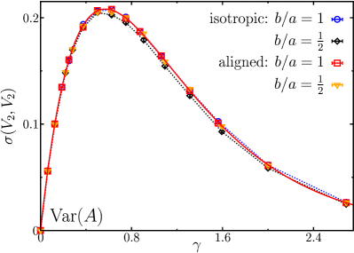
Refer to caption
Refer to caption
Refer to caption
Refer to caption
Refer to caption
Refer to caption
Figure 3: Variances and covariances of the intrinsic volumes V2subscript𝑉2V_{2} (area A𝐴A), V1subscript𝑉1V_{1} (proportional to perimeter P𝑃P), and V0subscript𝑉0V_{0} (Euler characteristic χ𝜒\chi) of Boolean models as a function of the intensity γ𝛾\gamma. Depicted are both numerical estimates in finite observation windows with periodic boundary conditions (marks with dotted lines as guides to the eye) and analytic curves of the covariances (solid lines), see Eqs. (42), (52), (54), (66), (71), and (76). Four different Boolean models are simulated: both for squares (b/a=1𝑏𝑎1{b}/{a}=1) and rectangles (b/a=1/2𝑏𝑎12{b}/{a}={1}/{2}) either an isotropic orientation distribution is used or the grains are aligned with the x𝑥x-direction. In the insets, the covariances and the variance of the perimeter of the Boolean model are rescaled by the perimeter of a single grain. In contrast to Fig. 2, the unit of area is the size of a single grain, that is v2=ab=1subscript𝑣2𝑎𝑏1v_{2}=ab=1.

For each sample m{1,Ms}𝑚1subscript𝑀𝑠m\in\{1,\dots M_{s}\} of a Boolean model, we determine the intrinsic volumes Vi(m)superscriptsubscript𝑉𝑖𝑚V_{i}^{(m)} (i=0,1,2𝑖012i=0,1,2). The sample covariance then provides an estimate for the covariance between the Minkowski functionals:

s(Vi,Vj):=1Ms1m=1Ms(Vi(m)Vi)(Vj(m)Vj)assign𝑠subscript𝑉𝑖subscript𝑉𝑗1subscript𝑀𝑠1superscriptsubscript𝑚1subscript𝑀𝑠superscriptsubscript𝑉𝑖𝑚delimited-⟨⟩subscript𝑉𝑖superscriptsubscript𝑉𝑗𝑚delimited-⟨⟩subscript𝑉𝑗s({V_{i},V_{j}}):=\frac{1}{M_{s}-1}\sum_{m=1}^{M_{s}}(V_{i}^{(m)}-\langle{}V_{i}{}\rangle)(V_{j}^{(m)}-\langle{}V_{j}{}\rangle)

using the sample mean Vi:=1Msm=1MsVi(m)assigndelimited-⟨⟩subscript𝑉𝑖1subscript𝑀𝑠superscriptsubscript𝑚1subscript𝑀𝑠superscriptsubscript𝑉𝑖𝑚\langle{}V_{i}{}\rangle:=\frac{1}{M_{s}}\sum_{m=1}^{M_{s}}V_{i}^{(m)} as an estimator for the expectation. In accordance with the definition of the asymptotic covariances in Theorem 3.1, the sample covariance is then divided by the size L2superscript𝐿2L^{2} of the observation window. We finally use bootstrapping (with 100010001000 bootstrap samples) to estimate the mean and the error of the estimators.

Figure 3 shows the simulation results for the variances and covariances of the intrinsic volumes for an isotropic orientation distribution of the grains as well as for aligned rectangles. In the latter case, the simulation results are compared to the analytic results in Eqs. (42), (52), (54), (66), (71), and (76). They are in excellent agreement.
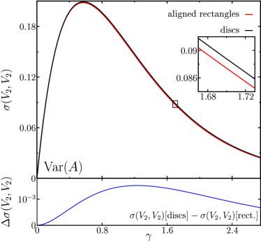
Refer to caption
Refer to caption


Refer to caption Refer to caption

Figure 4: Variances and covariances: σ(V2,V2)𝜎subscript𝑉2subscript𝑉2\sigma(V_{2},V_{2}), the variance of the area; σ(V1,V2)/v1𝜎subscript𝑉1subscript𝑉2subscript𝑣1\sigma(V_{1},V_{2})/v_{1}, proportional to the covariance of area and perimeter; v1subscript𝑣1v_{1} is half of the perimeter of a single grain; σ(V1,V1)/v12𝜎subscript𝑉1subscript𝑉1superscriptsubscript𝑣12\sigma(V_{1},V_{1})/v_{1}^{2}, proportional to the variance of the perimeter; σ(V0,V2)𝜎subscript𝑉0subscript𝑉2\sigma(V_{0},V_{2}), the covariance of area and Euler characteristic; σ(V0,V0)𝜎subscript𝑉0subscript𝑉0\sigma(V_{0},V_{0}), the variance of the Euler characteristic; σ(V0,V1)/v1𝜎subscript𝑉0subscript𝑉1subscript𝑣1\sigma(V_{0},V_{1})/v_{1}, proportional to the covariance of perimeter and Euler characteristic. They are shown both for Boolean models with aligned rectangles, see Eqs. (42), (52), (54), (66), (71), and (76), and for overlapping discs, see HLS . Note that except for σ(V1,V1)/v12𝜎subscript𝑉1subscript𝑉1superscriptsubscript𝑣12\sigma(V_{1},V_{1})/v_{1}^{2} the curves for the rectangles are independent of the aspect ratio of the rectangle, see also Figs. 2 and 3. The insets in the figures at the top are close-up views which show that the covariances differ slightly for Boolean model with rectangles or with discs. Below each subfigure, the differences of the covariances for Boolean models with rectangles or discs are plotted.

The variances and covariances of the Minkowski functionals of overlapping rectangles exhibit a complex behaviour as functions of the intensity γ𝛾\gamma similar to the Boolean model with discs in (HLS, , Section 7). The variances of area and Euler characteristic apparently have one maximum and no other extrema. The variance of the perimeter has a global maximum and (at least) one local minimum. As expected, the three Minkowski functionals are positively correlated at low intensities γ𝛾\gamma, but at relatively high intensities the area is anti-correlated to both the Euler characteristic and the perimeter.

The covariance σ(V0,V1)𝜎subscript𝑉0subscript𝑉1\sigma(V_{0},V_{1}) between the perimeter and the Euler characteristic shows a qualitatively different behaviour for rectangles with an isotropic orientation distribution when compared to the overlapping discs or aligned rectangles. There is a regime in the intensity γ𝛾\gamma (around the first local minimum) for which the rectangles with an isotropic orientation distribution are anti-correlated, while the aligned grains are positively correlated like the discs in HLS . This is probably related to the fact that rotated rectangles can more easily form clusters with holes than aligned rectangles or discs. The zero-crossing of the expectation of the Euler characteristic χ𝜒\chi for the rectangles with an isotropic orientation distribution is within this regime. For the aligned rectangles, the zero-crossing of the mean value of χ𝜒\chi is at the end of this regime, see HoerrmannHugKlattMecke .

The question remains whether or not the variances and covariances of area or rescaled perimeter of the Boolean model are independent of the grain distribution like the first moments of these functionals. Equations (42) and (52) show that at least for aligned rectangles the variance σ(V2,V2)𝜎subscript𝑉2subscript𝑉2\sigma(V_{2},V_{2}) as well as the covariance σ(V1,V2)𝜎subscript𝑉1subscript𝑉2\sigma(V_{1},V_{2}) divided by the perimeter of a single grain (2a+2b)2𝑎2𝑏(2a+2b) are indeed independent of the aspect ratio. The simulation results from Fig. 3 might suggest that this could also be valid for the isotropic orientation distributions. However, the variance σ(V2,V2)𝜎subscript𝑉2subscript𝑉2\sigma(V_{2},V_{2}) and the rescaled covariance σ(V1,V2)/(2a+2b)𝜎subscript𝑉1subscript𝑉22𝑎2𝑏\sigma(V_{1},V_{2})/(2a+2b) do depend on the grain distribution, although only weakly for the models studied here. To show this, we evaluate Eqs. (42) and (52) numerically and compare the covariances to those of the Boolean model with discs from HLS . Figure 4 shows that there is a weak but significant difference in the analytic curves of σ(V2,V2)𝜎subscript𝑉2subscript𝑉2\sigma(V_{2},V_{2}) and σ(V1,V2)𝜎subscript𝑉1subscript𝑉2\sigma(V_{1},V_{2}) for the two different models. The variance of the perimeter depends more clearly on the grain distribution. Even if it is rescaled by the perimeter of a single grain and even for aligned grains, the variance distinctly depends on the aspect ratio of the rectangles (except for small intensities γ𝛾\gamma). So, in contrast to the first moments of the area and rescaled perimeter of the Boolean model, the second moments in general depend on the grain distribution, e.g., the orientation distribution, even if this dependence may be weak. As expected, also the variance σ(V0,V0)𝜎subscript𝑉0subscript𝑉0\sigma(V_{0},V_{0}) of the Euler characteristic as well as the covariances σ(V0,V1)𝜎subscript𝑉0subscript𝑉1\sigma(V_{0},V_{1}) and σ(V0,V2)𝜎subscript𝑉0subscript𝑉2\sigma(V_{0},V_{2}) depend on the grain distribution, see Fig. 4.

6.2 Central limit theorem
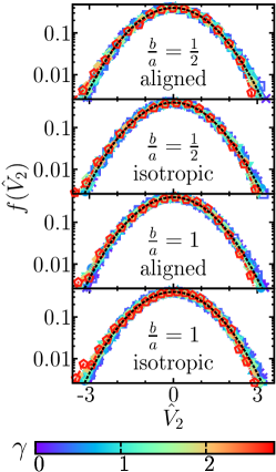
Refer to caption
Refer to caption
Refer to caption
Figure 5: Histograms f𝑓f of the normalized intrinsic volumes V^isubscript^𝑉𝑖\hat{V}_{i} (see Eq. (77)) of Boolean models of rectangles with different aspect ratios b/a𝑏𝑎b/a for different intensities γ𝛾\gamma; for both aligned rectangles and rectangles with an isotropic orientation distribution. For all of these different models, the rescaled distributions are already for the relatively small system size L=20a𝐿20𝑎L=20a in very good agreement with a normal distribution (dashed black line).

We also determine the histograms of the intrinsic volumes in a finite observation window, where the histograms are weighted by the total number of samples and the bin width. The histograms are then compared to the density of a standard normal distribution in order to numerically validate the central limit theorems in Section 4. The information content of a histogram is up to the binning almost equivalent to the empirical distribution function, but in plotting it is more convenient to compare histograms and densities.

The histograms resemble probability density functions. However, the intrinsic volumes of the considered Boolean model do not have probability density functions. Indeed, with positive probability, there is no overlap between the grains and there are no intersections with the boundary so that some multiples of the intrinsic volumes of the fixed grain have positive probability.

In this subsection, we simulate larger systems than in the previous Subsection 6.1. For a simulation box with side length L=20a𝐿20𝑎L=20a, we perform for each different set of parameters between Ms=5000subscript𝑀𝑠5000M_{s}=$5000$ and 150000150000150000 simulations of Boolean models with rectangles at varying intensities γ𝛾\gamma. Like in Subsection 6.1, the rectangles have aspect ratio 111 or 1/2121/2, and they are either aligned w.r.t. the observation window or their orientation is isotropically distributed. To produce the histograms, we simulate more than 140000014000001400000 samples of Boolean models including about 350000000350000000350000000 rectangles in total.

We normalize the intrinsic volumes Visubscript𝑉𝑖V_{i}, i.e., we subtract the estimated mean values Videlimited-⟨⟩subscript𝑉𝑖\langle{}V_{i}{}\rangle of the intrinsic volumes and divide by s(Vi,Vi)𝑠subscript𝑉𝑖subscript𝑉𝑖\sqrt{s(V_{i},V_{i})}:

V^i:=ViVis(Vi,Vi).assignsubscript^𝑉𝑖subscript𝑉𝑖delimited-⟨⟩subscript𝑉𝑖𝑠subscript𝑉𝑖subscript𝑉𝑖\displaystyle\hat{V}_{i}:=\frac{V_{i}-\langle{}V_{i}{}\rangle}{\sqrt{s(V_{i},V_{i})}}\;. (77)

Figure 5 plots the histograms f𝑓f of the normalized intrinsic volumes of Boolean models with different aspect ratios b/a𝑏𝑎b/a for either aligned rectangles or rectangles with an isotropic orientation distribution and for varying intensities γ𝛾\gamma.

These histograms are in good agreement with the density function of a normal distribution for all intrinsic volumes, for all intensities, and for all of the simulated models (despite the relatively small simulation box). In other words, even in small observation windows, the probability distributions of the intrinsic volumes of Boolean models can be well approximated by Gaussian distributions.

As we have mentioned in the introduction, the central limit theorems for the geometric functionals (see Theorems 4.1 and 4.2) and the exact formulae for the second moments (see Theorems 3.2 and 3.3) can be used for hypothesis testing of models of random heterogeneous media. A hypothesis test could, e.g., use the intrinsic volumes to decide whether or not a random two-phase medium can be modeled by overlapping grains. The joint probability distribution of the Minkowski functionals allows for a characterization of the shape by several geometrical functionals and hence for a construction of tests using their full covariance structure. For a different random field (with a Poisson distributed number of counts in a binned gamma-ray sky map) such a sensitive morphometric data analysis has already been developed GoeringKlattEtAl2013 ; KlattGoeringStegmannMecke2012 . The same concepts could be applied to the Boolean model.

In Fig. 5, there are only small deviations from a normal distribution relative to the error bars. So, the systematic deviations, e.g., due to the finite observation window size, seem to be small. In order to determine these deviations, a very high numerical accuracy is needed. We simulate 31063superscript1063\cdot 10^{6} samples of two Boolean models for rectangles with aspect ratio 1/212{1}/{2} that are either aligned or follow an isotropic orientation distribution. Here, we apply minus sampling boundary conditions, i.e., we consider all grains with centres in a slightly larger simulation box [a2+b2/2,L+a2+b2/2]2superscriptsuperscript𝑎2superscript𝑏22𝐿superscript𝑎2superscript𝑏222[-\sqrt{a^{2}+b^{2}}/2,L+\sqrt{a^{2}+b^{2}}/2]^{2}, but the observation window is still the original square (0,L)2superscript0𝐿2(0,L)^{2} with L=20a𝐿20𝑎{L}=20a. Contributions caused by the boundary are here neglected as it is often done in physics. The expected number of grains in the simulation box is adjusted accordingly and follows a Poisson distribution with mean γ(L+a2+b2)2𝛾superscript𝐿superscript𝑎2superscript𝑏22\gamma\cdot(L+\sqrt{a^{2}+b^{2}})^{2}. To minimize the computational costs, a relatively low intensity γ𝛾\gamma is chosen for these simulations. It corresponds to an expected occupied area fraction ϕ=1/15italic-ϕ115\phi={1}/{15}. The resulting histograms are plotted in Fig. 6. As expected, the high statistics reveal for the small system size deviations from the normal distribution that are significantly larger than the error bars.

For each underlying Boolean model, the histograms of the normalized intrinsic volumes coincide within error bars. This is not surprising because at the low intensity chosen here the intrinsic volumes are strongly correlated. (The correlation coefficients are larger than 0.9.)
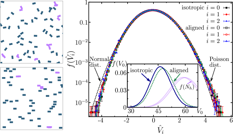
Refer to caption
Figure 6: Histograms f𝑓f of the normalized intrinsic volumes V^isubscript^𝑉𝑖\hat{V}_{i} (see Eq. (77)) of Boolean models with either aligned rectangles or rectangles with an isotropic orientation distribution. The dashed black line depicts the density of a normal distribution. On the left hand side, two samples of the Boolean models with either an isotropic orientation distribution or aligned rectangles are shown; clusters of rectangles are colored purple. The inset shows the histograms of the non-rescaled Euler characteristic V0subscript𝑉0V_{0} in the isotropic and aligned case as well as the corresponding probability mass functions of the number of grains Nhsubscript𝑁N_{h} hitting the observation window with mean values 59.459.459.4 and 60.560.560.5, respectively.

For different Boolean models (isotropic orientation distribution or aligned grains), the histogram of the non-rescaled Minkowski functionals differ slightly but distinctly already for the relatively small intensity studied here, see the inset of Fig. 6. In contrast to this, the histograms of the normalized intrinsic volumes collapse for the different Boolean models within the error bars to a single curve, which can be well approximated by a standardized Poisson distribution. This can be explained by the strong correlation between the intrinsic volumes and the number of grains Nhsubscript𝑁N_{h} hitting the observation window for each Boolean model. The latter follows a Poisson distribution with parameter 𝐄[Nh]=γ𝐄[V2([0;L]2+Z0)]𝐄delimited-[]subscript𝑁𝛾𝐄delimited-[]subscript𝑉2superscript0𝐿2subscript𝑍0\mathbf{E}[N_{h}]=\gamma\cdot\mathbf{E}[V_{2}([0;L]^{2}+Z_{0})]. (The correlation coefficients are larger than 0.85.) There is only a small relative difference between the parameters 𝐄[Nh]𝐄delimited-[]subscript𝑁\mathbf{E}[N_{h}] for the different considered Boolean models, because the observation window is large when compared to the typical grain Z0subscript𝑍0Z_{0}. Therefore, the corresponding Poisson distributions are very close after standardization (dashed green line in Fig. 6) and coincide with the histograms of the normalized intrinsic volumes.

Acknowledgements.
We would like to thank Julia Hörrmann and Klaus Mecke for some helpful remarks and discussions. The authors were supported by the German Research Foundation (DFG) through the research unit “Geometry and Physics of Spatial Random Systems”.

References

  • (1) Arns, C., Knackstedt, M., Mecke, K.: Reconstructing complex materials via effective grain shapes. Phys. Rev. Lett. 91, 1–4 (2003)
  • (2) Baryshnikov, Y., Yukich, J.E.: Gaussian limits for random measures in geometric probability. Ann. Appl. Probab. 15, 213–253 (2005)
  • (3) Baddeley, A.: A limit theorem for statistics of spatial data. Adv. in Appl. Probab. 12, 447–461 (1980)
  • (4) Brodatzki, U., Mecke K.: Simulating stochastic geometries: morphology of overlapping grains. Comput. Phys. Commun. 147, 218–221 (2002)
  • (5) CGAL, Computational Geometry Algorithms Library. http://www.cgal.org
  • (6) Chiu, S. N., Stoyan, D., Kendall, W. S., Mecke, J.: Stochastic Geometry and its Applications, Third Edition. Wiley, Chichester (2013)
  • (7) Davy, P.: Projected thick sections through multi-dimensional particle aggregates. J. Appl. Probab. 13, 714–722 (1976); Correction: J. Appl. Probab. 15, 456 (1978)
  • (8) Göring, D., Klatt, M. A., Stegmann, C., Mecke, K.: Morphometric analysis in gamma-ray astronomy using Minkowski functionals. Astron. Astrophys. 555, A38 (2013)
  • (9) Hall, P.: Introduction to the Theory of Coverage Processes. Wiley, New York (1988)
  • (10) Heinrich, L.: Large deviations of the empirical volume fraction for stationary Poisson grain models. Ann. Appl. Probab. 15, 392–420 (2005)
  • (11) Heinrich, L., Molchanov, I.S.: Central limit theorems for a class of random measures associated with germ-grain models. Adv. in Appl. Probab. 31, 283–314 (1999)
  • (12) Hörrmann, J.: The method of densities for non-isotropic Boolean models. PhD thesis, Karlsruhe Institute of Technology (2014)
  • (13) Hörrmann, J., Hug, D., Klatt, M. A., Mecke, K.: Minkowski tensor density formulas for Boolean models. Adv. in Appl. Math. 55, 48–85 (2014)
  • (14) Hörrmann, J., Weil, W., Valuations and Boolean Models. To appear in Lecture Notes in Mathematics ‘Tensor Valuations and their Applications in Stochastic Geometry and Imaging’, arXiv:1510.07910 (2015)
  • (15) Hug, D.: Measures, curvatures and currents in convex geometry. Habilitationsschrift, Albert-Ludwigs-Universität Freiburg (1999)
  • (16) Hug, D., Last, G., Schulte, M.: Second order properties and central limit theorems for geometric functionals of Boolean. Ann. Appl. Probab. 26, 73–135 (2016)
  • (17) Hug, D., Schneider, R.: Tensor valuations and their local versions. To appear in Lecture Notes in Mathematics ‘Tensor Valuations and their Applications in Stochastic Geometry and Imaging’, http://home.mathematik.uni-freiburg.de/rschnei/Tensorvaluations.Chap2.pdf (2016+)
  • (18) Kerscher, M., Mecke, K., Schmalzing, J., Beisbart, C., Buchert, T., Wagner, H.: Morphological fluctuations of large-scale structure: The PSCz survey. Astron. Astrophys. 373, 1–11 (2001)
  • (19) Klatt, M. A.: Morphometry of random spatial structures in physics. PhD thesis, FAU Erlangen-Nürnberg (2016)
  • (20) Klatt, M. A., Göring, D., Stegmann, C., Mecke, K.: Shape analysis of counts maps. AIP Conf. Proc. 1505, 737–740 (2012)
  • (21) Last, G., Penrose, M. D.: Fock space representation, chaos expansion and covariance inequalities for general Poisson processes. Probab. Theory Related Fields 150, 663–690 (2011)
  • (22) Last, G., Peccati, G., Schulte, M.: Normal approximation on Poisson spaces: Mehler’s formula, second order Poincaré inequalities and stabilization. To appear in Probab. Theory Related Fields (2016+)
  • (23) Last, G., Penrose, M. D.: Lectures on the Poisson Process. To be published by Cambridge University Press (2016+)
  • (24) Mase, S.: Asymptotic properties of stereological estimators for stationary random sets. J. Appl. Probab. 19, 111–126 (1982)
  • (25) Mecke, K. R.: Additivity, convexity, and beyond: applications of Minkowski functionals in statistical physics. In: Mecke, K. R., Stoyan, D. (eds.) Statistical Physics and Spatial Statistics. Lecture Notes in Physics 554, pp. 111–184. Springer, Berlin, Heidelberg (2000)
  • (26) Mecke, K. R.: Exact moments of curvature measures in the Boolean model. J. Stat. Phys. 102, 1343–1381 (2001)
  • (27) Mecke, K. R., Buchert, T., Wagner, H.: Robust morphological measures for large-scale structure in the universe. Astron. Astrophys. 288, 697–704 (1994)
  • (28) Mecke, K. R., Seyfried, A.: Strong dependence of percolation thresholds on polydispersity. Europhys. Lett. 58, 28–34 (2002)
  • (29) Mecke, K. R., Stoyan, D.: Morphological characterization of point patterns. Biometrical J. 47, 473–488 (2005)
  • (30) Mecke, K., Wagner, H.: Euler characteristic and related measures for random geometric sets. J. Stat. Phys. 64, 843–850 (1991)
  • (31) Meester, R., Roy, R.: Continuum Percolation. Cambridge University Press, Cambridge (1996)
  • (32) Miles, R. E.: Estimating aggregate and overall characteristics from thick sections by transmission microscopy. J. Microsc. 107, 227–233 (1976)
  • (33) Molchanov, I.S.: Statistics of the Boolean model: from the estimation of means to the estimation of distributions. Adv. in Appl. Probab. 21, 63–86 (1995)
  • (34) Molchanov, I.S.: Statistics of the Boolean Model for Practitioners and Mathematicians. Wiley, Chichester (1996)
  • (35) Peccati, G., Solé, J. L., Taqqu, M. S., Utzet, F.: Stein’s method and normal approximation of Poisson functionals. Ann. Probab. 38, 443–478 (2010)
  • (36) Penrose, M.D.: Gaussian limits for random geometric measures. Electron. J. Probab. 12, 989–1035 (2007)
  • (37) Schneider, R.: Convex Bodies: the Brunn-Minkowski Theory, Second edition. Encyclopedia of Mathematics and its Applications 151, Cambridge University Press, Cambridge (2014)
  • (38) Schneider, R.: Valuations on convex bodies—the classical basic facts. To appear in Lecture Notes in Mathematics ‘Tensor Valuations and their Applications in Stochastic Geometry and Imaging’, http://home.mathematik.uni-freiburg.de/rschnei/Tensorvaluations.Chap1.pdf (2016+)
  • (39) Schneider, R., Weil, W.: Stochastic and Integral Geometry. Springer, Berlin (2008)
  • (40) Scholz, C., Wirner, F., Klatt, M. A., Hirneise, D., Schröder-Turk, G. E., Mecke, K., Bechinger, C.: Direct relations between morphology and transport in Boolean models. Phys. Rev. E 92, 043023 (2015)
  • (41) Schröder-Turk, G. E., Kapfer, S. C., Breidenbach, B., Beisbart, C., Mecke, K.: Tensorial Minkowski functionals and anisotropy measures for planar patterns. J. Microsc. 238, 57–74 (2010)
  • (42) Schröder-Turk, G. E., Mickel, W., Kapfer, S. C., Klatt, M. A., Schaller, F. M., Hoffmann, M. J. F., Kleppmann, N., Armstrong, P., Inayat, A., Hug, D., Reichelsdorfer, M., Peukert, W., Schwieger, W., Mecke, K.: Minkowski tensor shape analysis of cellular, granular and porous structures. Adv. Mater. 23, 2535–2553 (2011)
  • (43) Schröder-Turk, G. E., Mickel, W., Kapfer, S. C., Schaller, F. M., Breidenbach, B., Hug D., Mecke, K.: Minkowski tensors of anisotropic spatial structure. New J. Phys. 15, 083028 (2013)
  • (44) Torquato, S.: Random Heterogeneous Materials. Springer, Heidelberg (2002)