Certified Randomness from a Two-Level System in a Relativistic Quantum Field
Abstract
Randomness is an indispensable resource in modern science and information technology. Fortunately, an experimentally simple procedure exists to generate randomness with well-characterized devices: measuring a quantum system in a basis complementary to its preparation. Towards realizing this goal one may consider using atoms or superconducting qubits, promising candidates for quantum information processing. However, their unavoidable interaction with the electromagnetic field affects their dynamics. At large time scales, this can result in decoherence. Smaller time scales in principle avoid this problem, but may not be well analysed under the usual rotating wave and single-mode approximation (RWA and SMA) which break the relativistic nature of quantum field theory. Here, we use a fully relativistic analysis to quantify the information that an adversary with access to the field could get on the result of an atomic measurement. Surprisingly, we find that the adversary’s guessing probability is not minimized for atoms initially prepared in the ground state (an intuition derived from the RWA and SMA model).
I Introduction
Randomness is a fundamental resource for tasks as varied as numerical simulations, cryptography, algorithms or gambling Metropolis and Ulam (1949); Motwani and Raghavan (1995). It is known that quantum systems can be used to generate truly unpredictable outcomes. While measurements on entangled states allow one to certify this randomness under a small set of assumptions Pironio et al. (2010), measurements on single systems can already produce certified randomness if a higher “level of characterization” is taken into consideration Law et al. (2014). Here, we consider the randomness that can be certified by measuring a single atom in the latter case.
Atoms do not exist isolated: They always, and unavoidably, interact with the electromagnetic field. If we want to use an atomic system as a source of randomness, for example by preparing a state in one basis and then measuring in a mutually unbiased basis, one has to consider that between the time of preparation () and the time of measurement (), the atom interacts with the field, thus effectively sharing some information with the field. If this information can be retrieved by an adversary having access to the field at a later time, it may compromise the unpredictability of the atom’s measurement result.
When the time between preparation and measurement is large decoherence may leave the atom in a mixed state, thus significantly impacting the efficiency of an atomic random number generator. One could hope to circumvent this problem by considering a short time between preparation and measurement. However, certifying randomness in this regime requires special care since relativistic effects are expected to influence the leading order contributions to the correlations between the atom and the field in this situation, in a similar manner as in the case of entanglement harvesting Valentini (1991); Reznik (2003); Reznik et al. (2005); Pozas-Kerstjens and Martín-Martínez (2015).
It has been discussed in the context of relativistic quantum information that atomic probes which interact with the electromagnetic field become, in general, entangled with these fields. This is true even when the dynamics of the atom-field system is dominated by vacuum fluctuations Reznik et al. (2005); Pozas-Kerstjens and Martín-Martínez (2015). These correlations are neglected in quantum optics when working under the usual rotating wave approximation (RWA) and the single mode approximation (SMA) Scully and Zubairy (1997) – two approximations which break the Lorentz covariance of the interaction theory and allow for causality violations and superluminal signalling Martín-Martínez (2015). However, since such correlations could be used by an adversary to guess the result of the atomic measurement, neglecting them potentially results in an underestimate of the adversary’s power.
In this article, we focus on the regime of short time between preparation and measurement, and take into account the fully relativistic111By relativistic, we mean here that the detector is locally coupled to a Lorentz covariant field. This excludes any possibility of superluminal signalling (present within the SMA and RWA) Martín-Martínez (2015) and guarantees a proper description of high frequency modes relevant at short times. light-matter interaction model. Our analysis applies for instance to the case of an atomic probe in an optical cavity or free space, or to a superconducting qubit coupled to a transmission line.
We show that, even for atoms in the ground state in the presence of vacuum, the field fluctuations drive the creation of field-atom entanglement at a significant level. This implies, perhaps contrary to intuition, that reducing the time from preparation to measurement generally does not spare a decrease in the randomness extractable from the atom, even for extremely short timescales. We hence conclude that relativistic effects need to be taken into account in the short time regime.
We also show that, even for relatively long waiting times between preparation and measurement, the ground state of the atom together with the vacuum state of the field is not the optimal state for randomness extraction when all relativistic considerations are factored in. This contradicts the intuition stemming from the SMA and RWA according to which, if an atom starts in its ground state and the field is not excited, then the atom would not get entangled with the field, and so it would share no information with the field. Thus, our results demonstrate that the actual behavior is really different from the one given by these usual approximations. Quantitatively, for typical timescales and coupling regimes of strong and ultra-strong coupling in quantum optics and superconducting qubits in transmission lines, we estimate that that the use of the SMA and RWA leads to an overestimation of the amount of randomness that can reach magnitudes of the order of 10%.
II Quantifying the randomness extractable from an atomic detector
We consider the situation in which a user wants to generate random bits by performing a quantum measurement on an atom. For this purpose, he prepares the atom in a state , and then performs an optimal von Neumann measurement on it (e.g. in a complementary basis)222We leave the question of performing more general POVMs, possibly by involving additional ancillas Law et al. (2014), for further study. This could potentially certify up to two bits of randomness per measurement Acín et al. .. Since the measurement is not performed simultaneously with the state preparation, this leaves some time for the atom to interact with the electromagnetic field between its preparation and measurement (c.f. Fig. 1). In particular, this interaction modifies the optimal measurement to be performed at time with respect to the initial mutually unbiased measurement.
Typically, this joint evolution results in the state of the atom and the field being partially entangled. After this interaction, the field thus contains some information about the outcome observed by the user upon measurement of the atom. Assuming that the field is not fully under control of the user, but can eventually be accessed by someone interested in guessing the outcome of the atom measurement (i.e. an adversary), one must evaluate how much information about the atom’s state was shared with the field during this interaction time in order to certify the amount of randomness that can be extracted from the atom’s measurement. We now describe this computation.
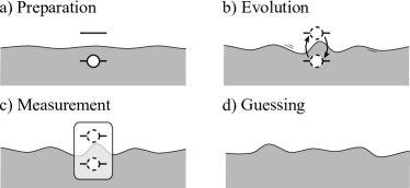
Let us consider a two-level atom and a massless scalar field in 1+1 dimensions initially prepared in the state . We model the atom-field interaction via a derivative coupling given by the following interaction Hamiltonian in the interaction picture
| (1) |
where is the coupling strength, the spatial profile of atom positioned at (henceforth assumed symmetric about ), the coupling switching function and the atom’s monopole moment. This is a simplified version of the light-matter interaction — it can be thought of as a polarization-insensitive direct coupling to the electric field which is the derivative of the vector potential in a 1D cavity such an optical fibre. The derivative coupling has been employed in the past to ameliorate the IR behaviour of the model in many different contexts Davies and Ottewill (2002); Wang and Unruh (2014); Juárez-Aubry and Louko (2014). In our case, the use of this model also allows us to minimize the impact of neglecting the zero-mode dynamics in case of the periodic cavity Martín-Martínez and Louko (2014). While simple, this family of Unruh-DeWitt detector models have been proved to capture the fundamental features of the light-matter interactions Alhambra et al. (2014); Martín-Martínez et al. (2013).
Notice, however, that despite its simplicity, the model we consider here fully describes the phenomenology of the light-matter interaction Scully and Zubairy (1997) assuming neither the RWA nor the SMA. As a consequence, this interaction model is a causally well-behaved theory Martín-Martínez (2015). This is crucial in the current context, where we expect vacuum correlations to play a role in the amount of randomness that can be extracted by measuring an atomic system in short times after preparation. Also, notice that the model does not consider the atom as a point-like particle but incorporates its spacial profile. Although the results are largely independent of the particular profile of the detector, its inclusion makes the analysis more general.
After the interaction with the field, the global state is given by
where represents time ordering.
After a time , the atom is measured in some basis. The global pure state of the atom and field then effectively ‘collapses’ into a state of the form with probability . Here, is the result of the measurement and is the state in which the field is left when the measurement result is , for a von Neumann measurement . This part of the state is the one that an adversary Eve could get in contact with, and eventually measure in order to infer the value of .
The amount of randomness that can be extracted from the outcome of the measurement performed at time with respect to an adversary having access to the quantum field can be quantified by the conditional min-entropy
| (2) |
where is the probability that the outcome (random variable) is guessed correctly given the state of the quantum field , and . Note that from a mathematical standpoint, the infinite-dimensionality of the quantum field as side information may a priori require some special care Berta et al. (2016). The interpretation of the min-entropy in this context, as well as its characterizing properties, remain however intact. Using the invariance of the conditional min-entropy under local isometries and the fact that the atom under consideration can only be excited in a finite number of levels, we can effectively treat the quantum field as a finite dimensional system. For this, we consider the state of the atom and field just before the von Neumann measurement. By the Schmidt decomposition, there exists a basis of the quantum field in which this state can be written as . An isometry can be set up between the field and an arbitrary qubit of Eve so that all the entanglement between and can be transferred to . We can thus compute the min-entropy on where is the qubit state hold by Eve whenever the atom is projected into outcome .
To arrive at an analytic expression for the min-entropy, we recall two facts. First, the guessing probability for cq states can be interpreted as the optimal success probability for Eve to distinguish the (normalized) ensemble of states :
where optimizing over TPCPMs is equivalent to optimizing over POVMs . Second, the optimal success probability for distinguishing an ensemble consisting of only two states is given be the Holevo-Helstrom theorem. Hence we find that the conditional min-entropy is given by
The measurement providing the largest amount of randomness from the atom can be found by optimization over all von Neumann measurements, namely . One can check that the result of this optimization can be expressed in terms of the purity of the reduced density-matrix only as
| (3) |
To see this, note that given the assumed form of and orthogonal projection with , , the operators and can be explicitly computed
which gives
Finally, it is useful to note that the fidelity between and reaches its maximum at .
The computation of the conditional min-entropy thus reduces to a computation of the reduced atomic state after the interaction with the quantum field. This is the subject of the next subsections.
II.1 The final atomic state from perturbation theory
For small enough values of the coupling strength , the time-evolved density matrix is well approximated by the following perturbative expansion:
| (4) |
where and are the first and second order perturbation terms in , and
| (5) |
Since we are going to consider three different boundary condition scenarios (free space, Dirichlet (reflective) cavities and periodic cavities), we will give the full detail of the calculations for the continuum case and skip directly to the final results for periodic and Dirichlet cavities.
For the case of a field in free space (e.g. an open optical fibre or open transmission line) the field can be expanded in plane-wave modes as
| (6) |
so that the interaction Hamiltonian becomes
where is the Fourier transform of the atomic spatial profile. We trace out the field to obtain the time-evolved state of the atom. The first order contribution to the time-evolved density matrix is traceless on the field for our initial state, therefore for an initial detector state given by
| (7) |
and choosing a matrix representation such that
| (8) |
the second order contributions in (4) are given by
Thus, the final state of the atom up to second order in perturbation theory is
| (9) |
where we define for
| (10) |
For atoms inside a cavity of length , the field modes are no longer continuous but discrete. More specifically, for periodic boundary conditions (e.g. a closed optical fibre loop) we can make the following replacements
| (11) | |||
| (12) |
while for Dirichlet cavity (e.g. reflective walls)
| (13) | |||
| (14) |
Moreover, we make the physical assumption that the atom is much smaller than the size of the cavity, allowing us to simplify
for a periodic cavity and similarly
for a Dirichlet cavity.
The form of the final state up to second order pertubation remains unchanged, and and now take the following form
| (15) |
| (16) |
II.2 For comparison: The final atomic state under the single mode and rotating wave approximations
When the coupling strength is small, it is frequent in quantum optics to simplify the interaction Hamiltonian (1) to the Jaynes-Cummings model where the single mode (SMA) and rotating wave (RWA) approximations are carried out when the atomic frequency is close to resonance with one of the cavity modes Scully and Zubairy (1997). We discussed in the introduction that these two approximations yield non-relativistic models for light matter interaction. In this paper we will compare the predictions of extracted randomness of the fully relativistic calculation with the prediction of the usual RWA SMA prediction in the Jaynes-Cummings model.
One may wonder why in this paper we do not analyze the SMA and RWA separately, and that perhaps only performing one of these two approximations could lead to valid results in the regimes that we are studying. However, we note that these two approximations are not independent, and in fact they derive from the same assumption: long evolution time as compared to the inverse of the atomic frequency gap. Moreover, in both approximations we neglect terms which are of the same order of magnitude, so it would be inconsistent to consider either of them individually (see Appendix A). Therefore, it makes sense to either do both approximations jointly (as we do in this section) or none of them (as we did in the previous section).
For the purpose of the comparison we suppose that the atom is on resonance with the () mode of the cavity, namely for periodic cavity and for Dirichlet cavity (which can be obtained by controlling the cavity’s length). With , as the resonant standing wave mode of the periodic cavity, the interaction Hamiltonian under RWA and SMA becomes
for a periodic cavity, and
for a Dirichlet cavity. This model can be solved exactly for all times, yielding the final state
where
and therefore the predictions of the SMA-RWA Jaynes-Cummings model can be compared with the fully relativistic model within the perturbative regime. More precisely, we use the following second order expansion of the previous final state
| (17) |
in the comparison.
III Simulation results
III.1 The concrete simulation model
Between the instant the atom is prepared in the state and its measurement, the atom interacts with the field for a duration in a manner that can be captured by the sharp switching function
| (18) |
We assume that the atom has the following simple spatial profile:
| (19) |
where gives the characteristic lenghtscale of the atomic species. Under these conditions, we have
where the notation refers to either the upper or the lower combination of signs to be taken on the right hand side (the same for the others). Given these expressions, the final state after the interaction (9) can be numerically approximated with high accuracy by performing the numerical integration or numerical summation up to a cutoff . Here, we normalize the numerical cutoff by the atomic’s size . Since the Fourier transform of the spatial profile is a Gaussian centered at zero with standard deviation proportional to , taking already gives an extremely precise numerical approximation, independently of the atom’s size.
III.2 Randomness certification in free space
From the final states computed in the previous sections, one can compute the number of random bits that can be extracted per atom measurement using Eq.(3). In Fig. 2 we report the result of this computation for the free field case (i.e. using Eq.(9),(10)).
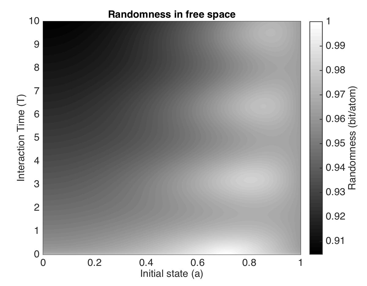
A first clear observation from Fig. 2 is that for most initial states, the randomness rate quickly decreases from 1 as soon as (see also solid line in Fig. 3). This shows that high-frequency terms play an important role in the evolution of the state for short times, and therefore they cannot be neglected.
One expected result that is verified in Fig. 2 is that preparing the atom in an excited state () always gives less randomness, at all interaction times within the limits of pertubation theory, than preparing it in the ground state. The reason for this behavior is clear: an atom in the excited state can be de-excited by the rotating wave terms in the interaction Hamiltonian with an elevated probability by emitting real field quanta. For short times, these field quanta are therefore correlated with the state of the atom, giving away information about the atomic state to an adversary having access to the quantum field. Conversely, an atom in the ground state () can only be correlated with the field via the counter-rotating part of the Hamiltonian. Even though in that case the atom also gets correlated with the field through vacuum fluctuations, the excited state is always less secure. This behavior is indeed expected from the non-relativistic intuition that an excited atom may emit a photon that an adversary can capture and learn about the state of the atom.
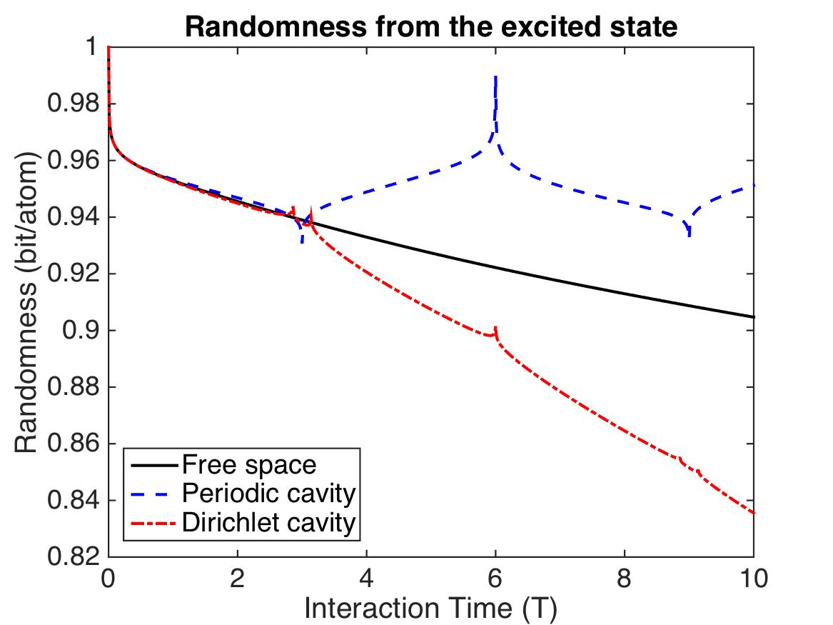
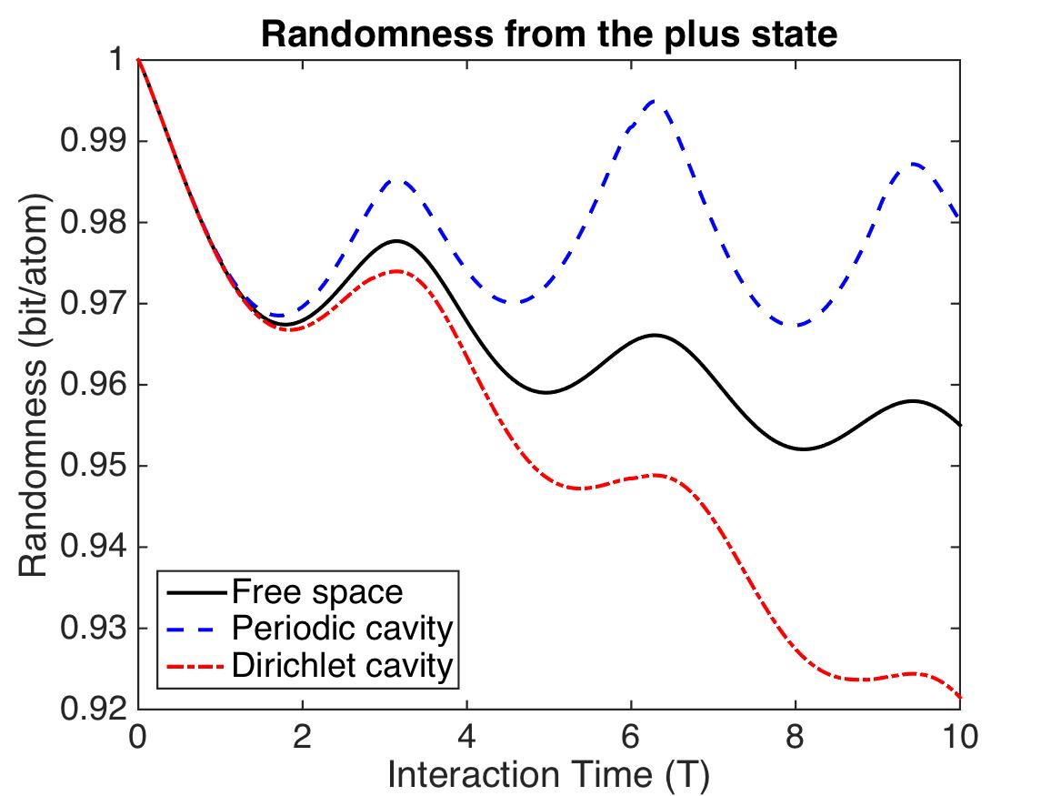
However, Fig. 2 also reveals a less intuitive effect. Namely, the ground state is not always the optimal state to extract randomness: depending on the other parameters, most notably the lag time between preparation and measurement , it may be better to prepare the atom in a superposition of ground and excited state (see also solid line in Fig. 3).
It is clear that the ground state cannot be fully secured, because it is not an eigenstate of the interaction Hamiltonian. Therefore the interaction introduces correlations between the atom and the field even when starting from the ground state. These correlations can later be used by an adversary (that does not need to be in light-contact with the first atom) to learn about the result of a measurement on the original atom. An example of how an adversary can gain information about the outcome of measurements even without receiving any energy from it is the ‘quantum collect calling’ (virtual-photon mediated timelike communication) Jonsson et al. (2014, 2015); Blasco et al. (2015).
It is worth noting that the randomness certified when starting from the ground state, after rapidly decreasing, seems to attain an asymptotic value (see Fig 3). While it is out of the scope of the present paper, it may constitute an interesting follow-up work to check whether this is still the case in the long time regimes, or whether non-perturbative effects may still significantly change the purity of the reduced state of the atom for long times.
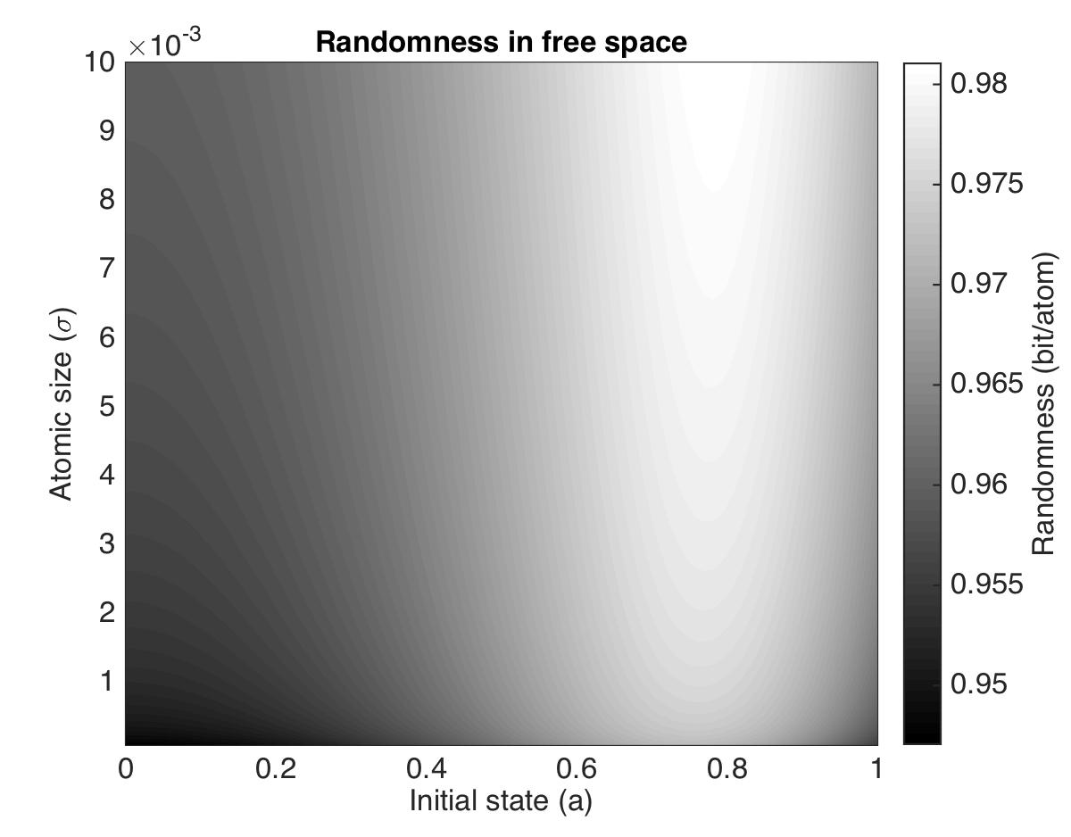
In Fig. 4, we study the effect of the atomic size on the certified randomness. One observes that more randomness is certified in presence of large atoms. The reason for this is that the bigger the atom gets the less the atom couples to the highest frequencies of the field, so the less the initial state is affected. Notice that the single mode approximation is recovered here when the atom is taken to be infinitely large and, thus, couples to a single frequency. This case, of course, breaks the relativistic approach (the single mode approximation strongly violates causality Jonsson et al. (2014)) which is not surprising since the atom sees the field at all points in space at the same time. In this case, the amount of certified randomness is essentially uniform over all states.
III.3 Randomness extraction in cavity
Atoms inside cavities are a more realistic experimental scenario compared to atoms in free space Raimond et al. (2001); Haroche (2013); Guerlin et al. (2007); Gleyzes et al. (2007); Brune et al. (1990); Nougues et al. (1999). There are two main differences when atoms are put inside a cavity. Firstly, the cavity only supports a countable infinite number of modes, as opposed to the continuously many modes in free space. Secondly, although there are fewer modes to interact, the interaction may be made stronger than in free space Blais et al. (2004); Wallraff et al. (2004); Chiorescu et al. (2004); Peropadre et al. (2010).
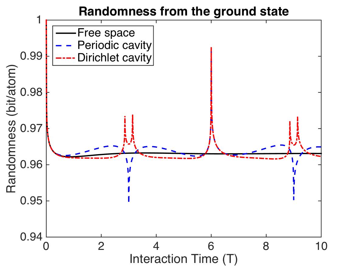
The resulting effect of these two differences on the guessing probability is presented in FIG. 3. The periodic and Dirichlet curves in this graph were obtained by computing Eq. (3) with Eq. (9),(15),(16). Notice that the length of the cavity in this case is three orders of magnitude larger than the size of the atom, so our physical assumption of a small atom in a large cavity is met. This figure also compares the randomness rate with respect to the one obtained in the free field case. The peaks in Fig. 3 correspond to the light-crossing time of the cavity (the perturbation caused by the switching of the interaction bounces back on the boundary of the cavity and returns to the atom).
One would expect that for larger and larger cavities, the two cavity results converge to the free space one. This is verified in Fig. 6.
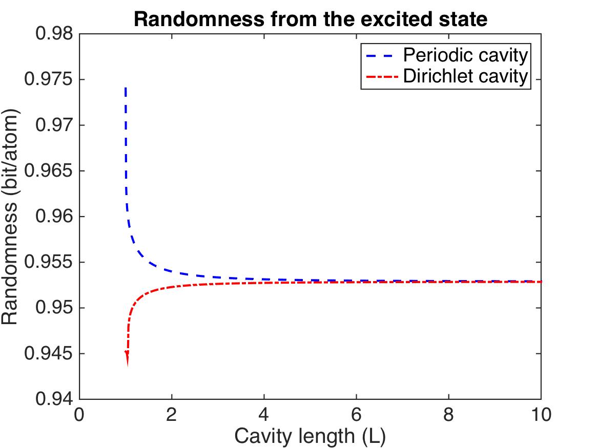
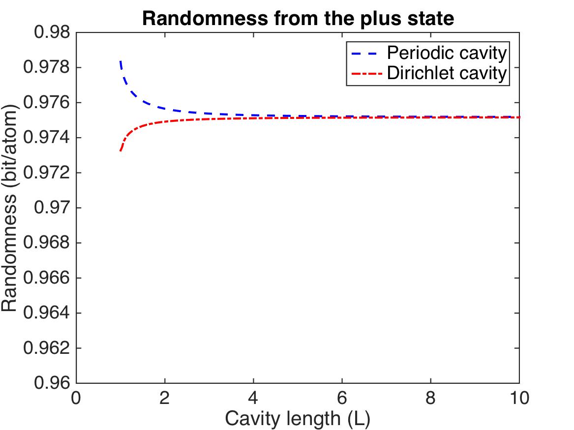
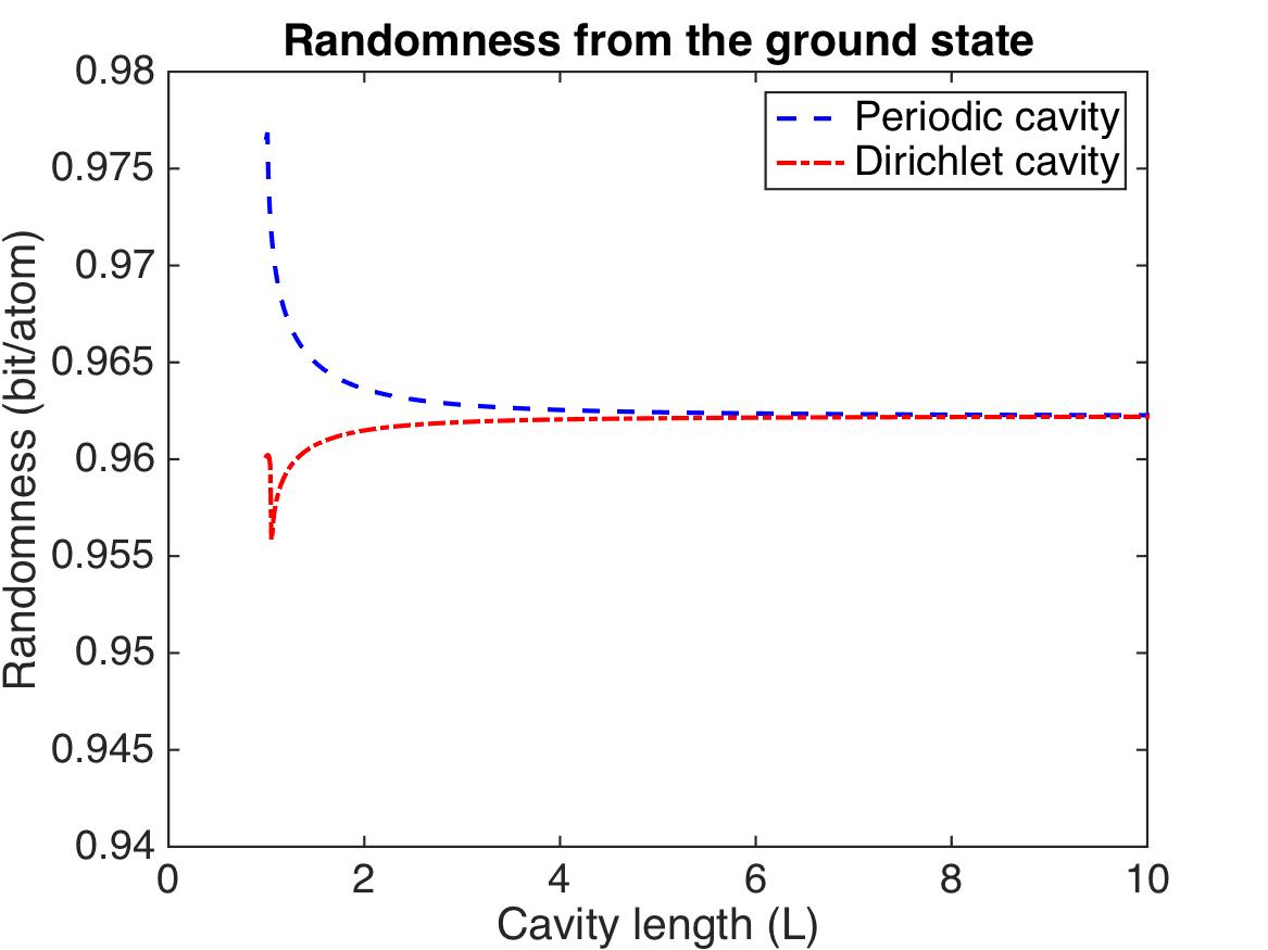
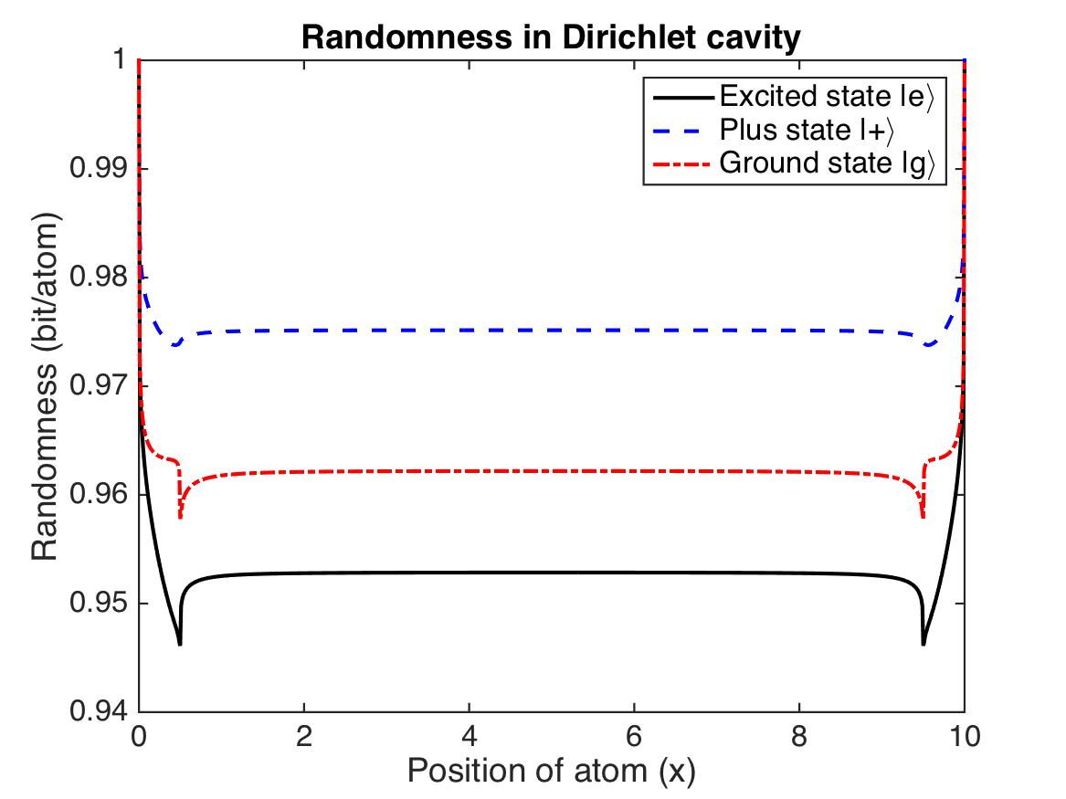
Also, in a Dirichlet cavity, the randomness output depends explicitly on the position of the atom, unlike in a periodic cavity. Fig. 7 shows that this dependence is negligible.
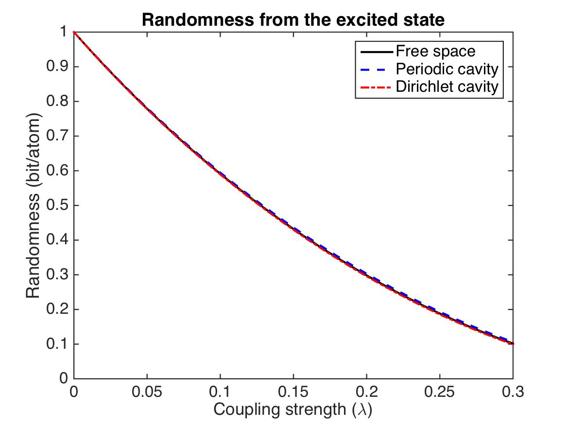
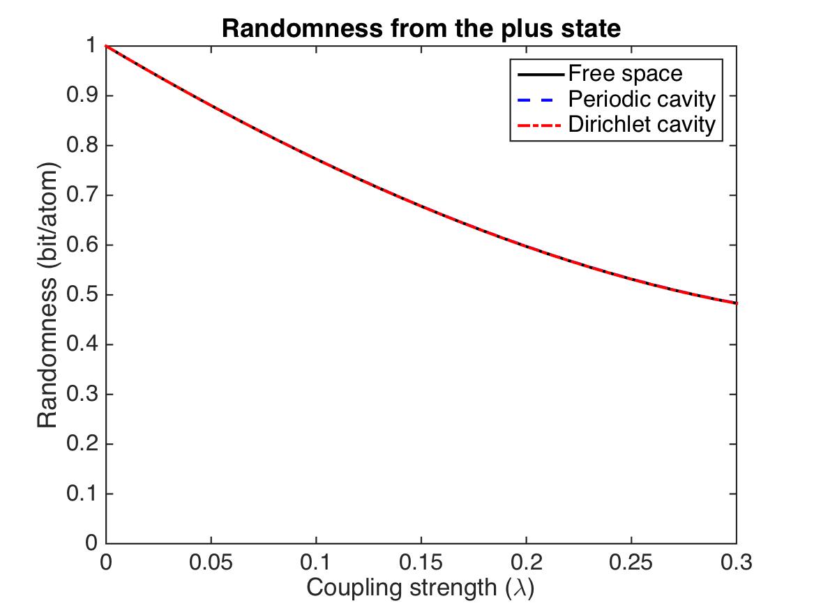
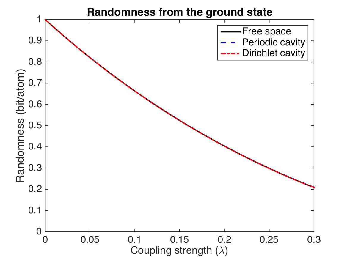
Finally, in Fig. 5 we analyse the role of the coupling strength on the randomness rate. We observe that the behavior is the same for all the boundary condition scenarios. This can be understood because we know from equation (3) that the min-entropy only depends on the purity of the final state , and from (1), (4) and (II.1), we see that the purity of the atomic state scales as for any set of boundary conditions.
III.4 Comparison with the rotating wave approximation
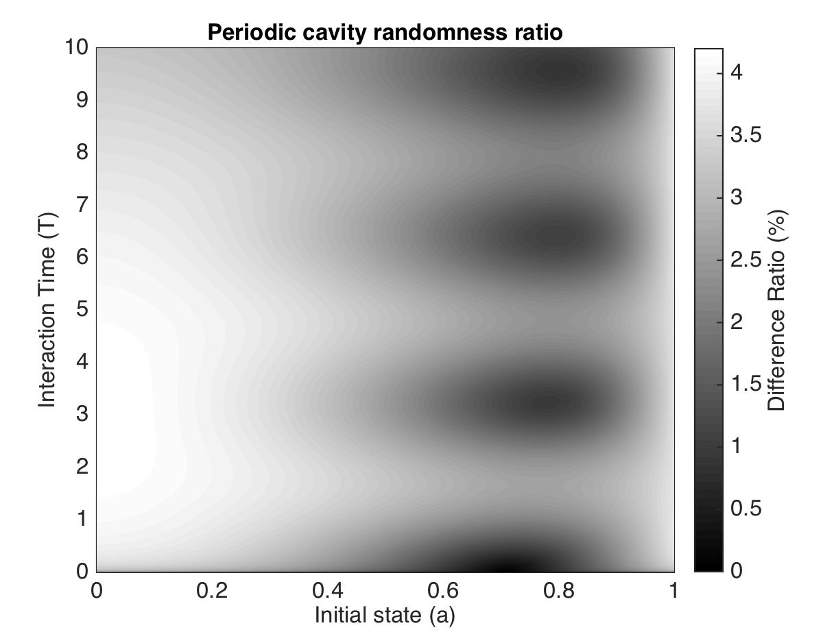
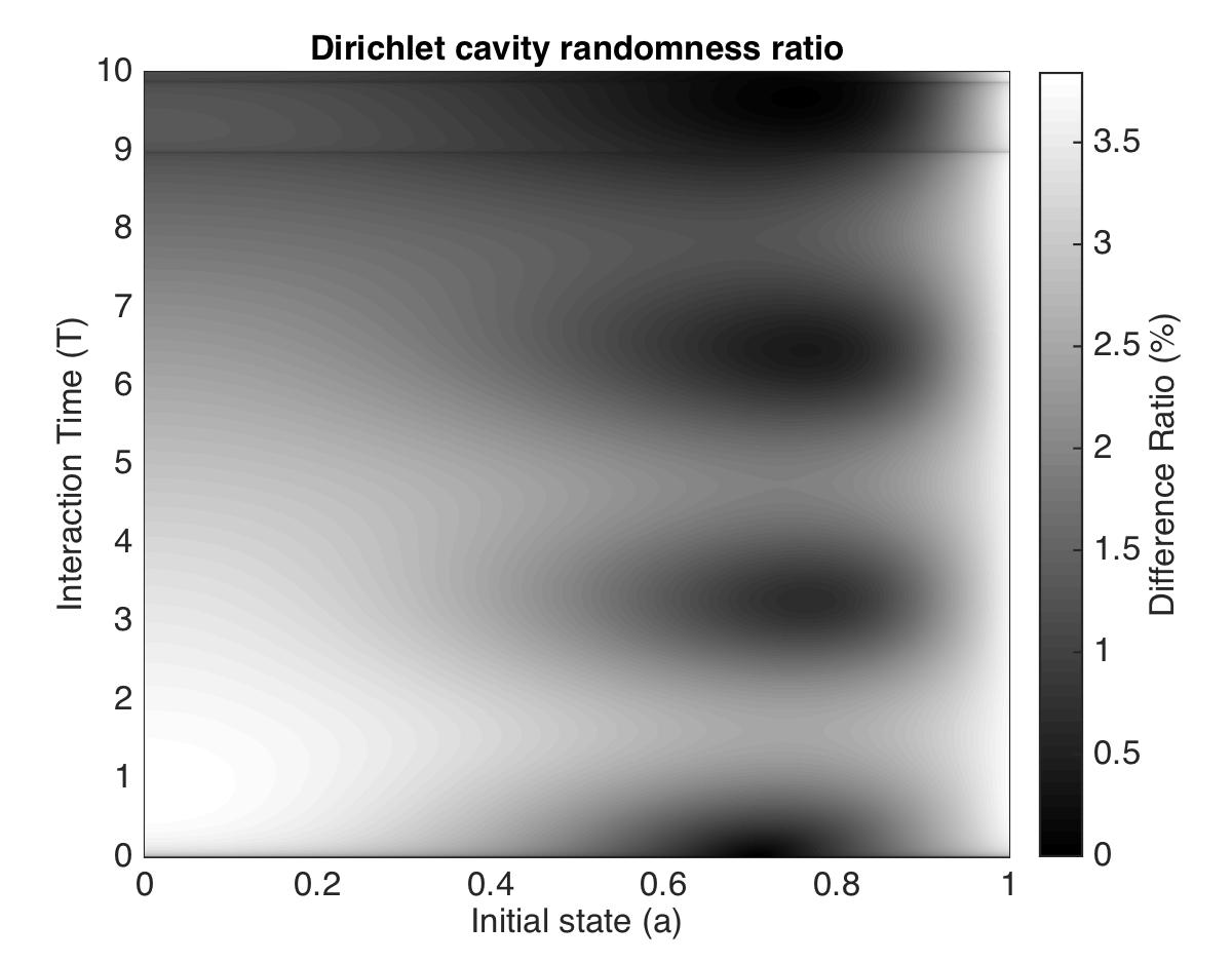
In order to compare the above results with predictions of the RWA model, we introduce the difference ratio
| (20) |
where is the randomness computed according the the method presented in the precedent paragraphs, i.e. from the state (9) with the terms described in Section III.1, and stands for the randomness computed directly from the state (17).
Since the RWA randomness is computed under the assumption that the atom is on resonant with some mode of the cavity, throughout this section, the length of the cavity is always fixed based on the chosen resonant mode according to for periodic cavity and for Dirichlet cavity. Note that for the sake of numerical simulation, cannot be chosen too small relative to because this violates the assumption of a relatively big cavity with respect to the atom’s size which we have made before.
As seen in the figure 8, the randomness obtained from the fully relativistic calculation is lower than the randomness computed from the rotating wave approximation model (i.e. ). We interpret this as coming from the fact that non-relativisitic approximations (SMA and RWA) neglect all the correlations created between the atomic probe and the remaining of the field modes. Indeed, the shorter the interaction, the larger the bandwidth of the field modes that get perturbed by the interaction (this can be thought as a consequence of a time-energy uncertainty).
IV Conclusions
In this paper we considered an atom coupled for a short time with the electromagnetic field. By taking into account the full relativistic description of the atom-field interaction, we studied the amount of information shared as a result of this interaction by the atom and the field beyond the rotating-wave and single-mode approximations, as quantified by the guessing probability. We showed that small waiting times between preparation and measurement do not rid the atomic system from the problem of starting to share information with the quantized electromagnetic field to which the atom is unavoidably coupled. This is in stark contrast to what the usual approximated models of light-matter interaction predict.
In particular, the Jaynes-Cummings model under the single-mode approximation and the rotating-wave approximation would predict that the optimal way to proceed to reduce this entanglement — and thus increase the randomness extractable from the atomic probe — would be to prepare the ground state of the atom and the field. This is easy to understand already from a classical intuition: If the atom is in the ground state and the field is not excited, the atom would remain in the ground state and thus it would not get correlated with the field. This intuition carries over to quantum optics under RWA and SMA. However, contrary to this intuition, we show that vacuum fluctuations entangle the atom with the field even in this case, and that this entanglement has significant consequences on the amount of certifiable randomness.
Also contrary to the classical intuition, we showed that the optimal amount of randomness is obtained for initial atomic states other than the ground state of the atom. This shows that the employment of the RWA and SMA in quantum optics does not provide a reliable lower bound on the amount of randomness that one can extract from an atomic probe.
As illustrative examples, we have analyzed the randomness loss due to these effects for the typical timescales and coupling regimes of strong and ultra-strong coupling in quantum optics and superconducting qubits in transmission lines, showing that the relative misestimation of the RWA and SMA models can indeed have a non-negligible magnitude.
Finally, our analysis suggests that the guessing probability as a function of the time of interaction converges to a constant value in some circumstances. If this result also carries to non-pertubative regimes this could allow for randomness certification independently of the interaction time. This is an interesting open question in its own right, and it will be studied elsewhere.
Appendix A Relation between the SMA and RWA
In this appendix, we discuss that the terms neglected by the SMA and RWA are of the same order. Therefore, both approximations are related.
Recall that we have a two-level atom interacting, according to Eq. (1), with a quantized quantum field in periodic or Dirichlet cavity with the form of given by Eq. (6) with the appropriate replacement rules. In this case, the dynamics is completely governed by the unitary time evolution operator which in the small coupling () is determined by Eq. (II.1). Let us assume further that the atom is on-resonant with the cavity mode for some fixed .
For illustration, the first order perturbation depends on terms of the form
| (21) |
where the terms with , corresponding to interaction terms of the form and , are usually called the rotating contributions, and the other terms where are called the counter-rotating contributions. Let us consider a constant interaction strength in some time interval . Namely in some and elsewhere. The contribution of the resonant mode to the qubit’s dynamics grows with while the off-resonant modes contribution stays bounded . The counter-rotating mode contributions are also always bounded .
Thus if one make the assumption of SMA, namely dropping all contributions from off-resonant modes (because their contributions stay bounded while that of the resonant mode grows with interaction time ), then for consistency one must drop the contributions from the counter rotating terms since they are smaller, i.e. doing RWA as well.
For both approximations to be faithful already at leading order in perturbation theory we need to demand that
-
•
There is a resonant mode
-
•
The interaction times are much larger than .
Since the requirement is the same for both approximations, it is not a consistent approach (in these simple light-matter interaction models) to consider one and not the other without any further hypotheses.
Acknowledgments
We thank Valerio Scarani, Jedrzej Kaniewski and Nicolas Sangouard for helpful discussions and correspondence. E. M-M. gratefully acknowledges Valerio Scarani for his hospitality during his visit to NUS-CQT.
This work is funded by the Singapore Ministry of Education (partly through the Academic Research Fund Tier 3 MOE2012-T3-1-009) and by the National Research Foundation of Singapore.
References
- Metropolis and Ulam (1949) N. Metropolis and S. Ulam, Journal of the American Statistical Association 44, pp. 335 (1949).
- Motwani and Raghavan (1995) R. Motwani and P. Raghavan, Randomized Algorithms (Cambridge University Press, New York, NY, USA, 1995).
- Pironio et al. (2010) S. Pironio, A. Acín, S. Massar, A. B. de la Giroday, D. N. Matsukevich, P. Maunz, S. Olmschenk, D. Hayes, L. Luo, T. A. Manning, and C. Monroe, Nature 464, 1021 (2010).
- Law et al. (2014) Y. Z. Law, L. P. Thinh, J.-D. Bancal, and V. Scarani, Journal of Physics A: Mathematical and Theoretical 47, 424028 (2014).
- Valentini (1991) A. Valentini, Physics Letters A 153, 321 (1991).
- Reznik (2003) B. Reznik, Found. Phys. 33, 167 (2003).
- Reznik et al. (2005) B. Reznik, A. Retzker, and J. Silman, Phys. Rev. A 71, 042104 (2005).
- Pozas-Kerstjens and Martín-Martínez (2015) A. Pozas-Kerstjens and E. Martín-Martínez, Phys. Rev. D 92, 064042 (2015).
- Scully and Zubairy (1997) M. O. Scully and M. S. Zubairy, Quantum Optics (Cambridge University Press, 1997).
- Martín-Martínez (2015) E. Martín-Martínez, Phys. Rev. D 92, 104019 (2015).
- (11) A. Acín, S. Pironio, and T. V. P. Wittek, ArXiv e-prints arXiv:1505.03837 [quant-ph] .
- Davies and Ottewill (2002) P. C. W. Davies and A. C. Ottewill, Phys. Rev. D 65, 104014 (2002).
- Wang and Unruh (2014) Q. Wang and W. G. Unruh, Phys. Rev. D 89, 085009 (2014).
- Juárez-Aubry and Louko (2014) B. A. Juárez-Aubry and J. Louko, Classical and Quantum Gravity 31, 245007 (2014).
- Martín-Martínez and Louko (2014) E. Martín-Martínez and J. Louko, Phys. Rev. D 90, 024015 (2014).
- Alhambra et al. (2014) A. M. Alhambra, A. Kempf, and E. Martín-Martínez, Phys. Rev. A 89, 033835 (2014).
- Martín-Martínez et al. (2013) E. Martín-Martínez, M. Montero, and M. del Rey, Phys. Rev. D 87, 064038 (2013).
- Berta et al. (2016) M. Berta, F. Furrer, and V. B. Scholz, J. Math. Phys 57, 015213 (2016).
- Jonsson et al. (2014) R. H. Jonsson, E. Martín-Martínez, and A. Kempf, Phys. Rev. A 89 (2014).
- Jonsson et al. (2015) R. H. Jonsson, E. Martín-Martínez, and A. Kempf, Phys. Rev. Lett. 114, 110505 (2015).
- Blasco et al. (2015) A. Blasco, L. J. Garay, M. Martín-Benito, and E. Martín-Martínez, Phys. Rev. Lett. 114, 141103 (2015).
- Raimond et al. (2001) J. M. Raimond, M. Brune, and S. Haroche, Rev. Mod. Phys. 73, 565 (2001).
- Haroche (2013) S. Haroche, Reviews of Modern Physics 85, 1083 (2013).
- Guerlin et al. (2007) C. Guerlin, J. Bernu, S. Deleglise, C. Sayrin, S. Gleyzes, S. Kuhr, M. Brune, J.-M. Raimond, and S. Haroche, Nature 448, 889 (2007).
- Gleyzes et al. (2007) S. Gleyzes, S. Kuhr, C. Guerlin, J. Bernu, S. Deleglise, U. B. Hoff, M. Brune, J.-M. Raimond, and S. Haroche, Nature 446, 297 (2007).
- Brune et al. (1990) M. Brune, S. Haroche, V. Lefevre, J. M. Raimond, and N. Zagury, Phys. Rev. Lett. 65, 976 (1990).
- Nougues et al. (1999) G. Nougues, A. Rauschenbeute, S. Osnaghi, M. Brune, J. M. Raimond, and S. Haroche, Nature 400, 239 (1999).
- Blais et al. (2004) A. Blais, R.-S. Huang, A. Wallraff, S. M. Girvin, and R. J. Schoelkopf, Phys. Rev. A 69, 062320 (2004).
- Wallraff et al. (2004) A. Wallraff, D. I. Schuster, A. Blais, L. Frunzio, R.-S. Huang, J. Majer, S. Kumar, S. M. Girvin, and R. J. Schoelkopf, Nature 431, 162 (2004).
- Chiorescu et al. (2004) I. Chiorescu, P. Bertet, K. Semba, Y. Nakamura, C. J. P. M. Harmans, and J. E. Mooij, Nature 431, 159 (2004).
- Peropadre et al. (2010) B. Peropadre, P. Forn-Díaz, E. Solano, and J. J. García-Ripoll, Phys. Rev. Lett. 105, 023601 (2010).