Chemical tagging can work:
Identification of stellar phase-space structures
purely by chemical-abundance similarity
Abstract
Chemical tagging promises to use detailed abundance measurements to identify spatially separated stars that were in fact born together (in the same molecular cloud), long ago. This idea has not yielded much practical success, presumably because of the noise and incompleteness in chemical-abundance measurements. We have succeeded in substantially improving spectroscopic measurements with The Cannon, which has now delivered individual abundances for stars observed as part of the APOGEE spectroscopic survey, with precisions around 0.04 dex. We test the chemical-tagging hypothesis by looking at clusters in abundance space and confirming that they are clustered in phase space. We identify (by the k-means algorithm) overdensities of stars in the 15-dimensional chemical-abundance space delivered by The Cannon, and plot the associated stars in phase space. We use only abundance-space information (no positional information) to identify stellar groups. We find that clusters in abundance space are indeed clusters in phase space. We recover some known phase-space clusters and find other interesting structures. This is the first-ever project to identify phase-space structures at survey-scale by blind search purely in abundance space; it verifies the precision of the abundance measurements delivered by The Cannon; the prospects for future data sets appear very good.
Submitted to The Astrophysical Journal
Section 1 Introduction
Ensembles of stars in the Milky Way are born in molecular clouds, which are presumed to be near-homogeneous in their chemical element composition. However, most stars are born in unbound associations, or are born in star clusters that disperse rapidly; they will eventually end up in very different parts of phase space in the Galaxy. Yet, if every star preserved its photospheric element abundances over its lifetime (at least for most elements), then stars of common birth origin ought to be identifiable through their detailed photospheric abundances, long after any spatial proximity has vanished.
This idea—dubbed “chemical tagging” (Freeman & Bland-Hawthorn, 2002; Bland-Hawthorn et al., 2010)—is one of the principal motivations for a number of surveys, including APOGEE (Majewski et al., 2015), Gaia–ESO (Gilmore et al., 2012) and GALAH (De Silva et al., 2015). In order to determine the precise abundance labels for chemical tagging, these surveys are each measuring high-resolution, high signal-to-noise () spectra for hundreds of thousands of stars across the Galaxy’s disk, bulge and halo.
Chemical tagging holds the promise of revealing not just the star-formation history of the Galaxy, but also the accretion history (as things that fall in are expected to be chemically distinct from those that form in the parent body; for example, Eggen 1970; Font et al. 2006; De Silva et al. 2007; Bubar & King 2010) and stellar-orbit diffusion processes like radial mixing and radial migration (for example, Roškar et al. 2008; Quillen et al. 2015). After stars are born—or after a star cluster is accreted and disrupted—associations or groups will disperse, through two-body mechanisms, interactions with resonances, or tides from the whole Galaxy.
Although undeniably promising—and motivating the launch of costly large-scale spectroscopic surveys—chemical-tagging as a search technique has yet to be proven in practice: identifying stars of common birth origin purely on the basis of their near-identical abundances patterns, without any consideration of position or velocity.
Part of the reason that chemical tagging remains unrealized is because the level of abundance specificity required is very high. If there are thousands of (relevant) molecular clouds forming stars in the recent history of the Milky Way, clumps of stars can only be identified in abundance space if abundance space is high in dimensionality. (In principle, it needs to be high in dimensionality both in terms of the number of measured abundances and in terms of the number of nucleosynthetic pathways or the dimensionality of the true abundance space.) Therefore accurate—or at least precise—measurements of many different abundances are needed for stellar siblings to have sufficiently unique fingerprints. Stellar spectroscopic surveys now have the resolution, , wavelength coverage, and sample sizes to deliver many different chemical tags for each star.
There are, however, two big issues. The first is that the physical assumptions behind the idea may require refinement: There may be chemical-abundance overlaps among open clusters (Blanco-Cuaresma et al., 2015), coeval groups of stars may have similar tags but different birth places (Mitschang et al., 2014), and the chemical-abundance space might be low in dimensionality. On the other hand, precise studies of stellar twins (Melendez et al., 2014; Jofré et al., 2015) indicate that pairs of stars can be found with unusually similar abundances, open clusters show remarkably uniform chemical abundances (Bovy, 2015), and peculiar abundance ratios have been successfully used to identify disrupted cluster members (for example, Majewski et al. 2012). There have also been hints seen of relationships between chemistry and kinematics (for example, Helmi et al. 2006, 2014).
The second issue for chemical tagging—and the one we address here—is measurement precision (and accuracy). The current precision on abundance measurements in the published survey catalogs is not high enough (for example, Martell 2015; Ting et al. 2016). However, our recent work (Ness et al., 2015) suggests that the data are precise enough: There is enough at the relevant locations in spectrum space to deliver high-precision tags. The existence of very large data sets, homogeneous in spectrum space, suggests that data-driven approaches to the determination of stellar abundances might considerably outperform traditional methods. These traditional approaches are based on ab-initio physical models that have shortcomings that become apparent in this age of high-quality spectra, and the data-analysis methods do not make use of all of the information in the data sets. Improving the models and exploiting the entire information content in the data is critical if we are going to deliver useful chemical tags.
Our specific contribution in this space has been to develop The Cannon (Ness et al., 2015, 2016a), which is a data-driven model for stellar spectra. This model can deliver stellar parameters and chemical abundances for stars, making use of every pixel of every stellar spectrum (that is, all the information in the data) but making no use at all of physical models of stars. It relies only on there being training data—some reference stars for which parameters and abundances are known and believed. In companion papers (Casey et al., 2016; Ness et al., 2016b) we show that The Cannon can deliver 15 to 19 abundances for stars in the APOGEE survey, at precisions higher than even the training (reference) data on which the model is trained. We say more about this below. We will show here that The Cannon improves chemical abundance measurements to the point that chemical tagging is now possible.
One note on accuracy and precision: In principle, the problem of chemical tagging does not require absolute accuracy for chemical-abundance measurements. It only requires that we can precisely see that two stars are similar in their abundances, even if we happen to be wrong about the absolute values of those abundances. This point might make it seem like we don’t care that our models are wrong, so long as they are consistent. However, this is a bit misleading: For chemical tagging to succeed, we need stars with different atmospheric parameters but the same chemical abundances to be assigned the same position in chemical-abundance space. That doesn’t require overall accuracy, but it requires that the models have the right dependencies on atmospheric parameters such that the wrongness in abundance space is consistent across the Hertzsprung-Russell diagram. That is, we need a substantial amount of accuracy to achieve our goals.
It is important to realize that analysis techniques based on ab-initio physical models are inaccurate, yet they too strive to improve precision in the face of knowingly inaccurate models. Incomplete atomic data, simplifications of photospheric structure, assumptions about convective motion, and inconsistencies resulting from positing local thermal equilibrium all contribute to produce inaccurate abundances. The Cannon stands out because it demonstrably improves the precision on chemical abundances, whereas the accuracy of those labels is limited only by the training (reference) set employed. At the same time, it is crucial to be cognisant of the constraints in the training set: the results of The Cannon will be limited by the quality of the training set labels. While chemical tagging does not necessarily require accurate abundance labels (precision is paramount), comparing abundance labels to models of Galactic chemical enrichment requires a firm level of belief in the label accuracy. Particularly for the abundance labels of stars in the training set.
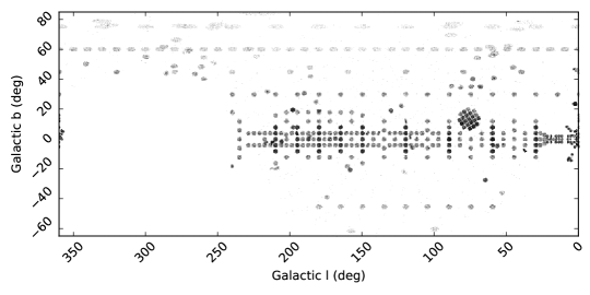
In what follows, we are going to use APOGEE DR12 data (Holtzman et al., 2015; Alam et al., 2015) from SDSS-III (Eisenstein et al., 2011), in which we can re-derive 15 element abundances (C, N, O, Na, Mg, Al, Si, S, K, Ca, Ti, V, Mn, Fe, Ni), using The Cannon (Ness et al., 2015). The APOGEE data set covers a huge radial extent and—because the data are taken in the infrared—is capable of exploring all parts of the disk, including the thin parts. However, it has the disadvantage that its spatial coverage is incomplete (that is, limited pointings produce a fractured sky map), which makes it hard to see, within the data set, linear or extended stellar structures. In many ways, GALAH will deliver improvements, both because it will have more abundances (possibly 29) and contiguous sky coverage (De Silva et al., 2015); that said, it will not observe much of the thin disk.
One final note: we think of this Article as performing a proof of concept. We know that the stellar members of open and globular clusters—stars that are identified by being close in phase space—contain highly informative abundance information that identifies them also in chemical-abundance space. Does this work the other way around? Can chemical tagging identify small subsets of stars, among a vastly greater background sample, that have a common birth origin? If we find stars purely by their clustering in abundance space and subsequently show that they are part of a still spatially coherent cluster, group, or stream, then we will have resolved all practical outstanding issues plaguing chemical tagging, thereby bringing us much closer to unravelling the formation of the Milky Way.
Section 2 Data: APOGEE giants with abundances from The Cannon
Our analysis draws on the spectra of 98,462 giant stars () from APOGEE DR12 (Holtzman et al., 2015), with no warning flags set in the APOGEE ASPCAP (García Pérez et al., 2015) pipeline reductions. We re-analyze these spectra using The Cannon, because it can deliver stellar abundance labels of higher precision, especially for stars of . The details about how we select, reduce, and analyze the APOGEE data are given in full detail in the companion papers (Casey et al., 2016; Ness et al., 2016b), and we only summarize briefly here: We re-derived 17 labels (, , and 15 abundances referenced to H) from the APOGEE DR12 spectra. For the training step of The Cannon, 12,681 red-giant stars with spectral were used. For this small fraction of the sample with the highest , the labels provided by ASPCAP provide consistent, relatively low-scatter, sensible abundance-space measurements. The training step fixes a spectral model that predicts the normalized spectrum as a quadratic function of all labels ( model coefficients). In the second stage—the test step—each unlabelled star is used to establish a single-star likelihood function for its labels, holding the spectral model coefficients (the parameters of the model) fixed. The Cannon finds the labels that minimize the single-star likelihood function for each test-set star. This optimization is not convex, but it is trivially parallel, and therefore fast. The test step for 150,000 spectra takes less than 30 minutes on a small research cluster in Cambridge.
It is important here to note some of the limitations of stellar labels delivered by The Cannon. The first is that The Cannon is only as good as its training set! All of the biases and calibration issues in the input training set will be delivered to the output labels. This means that there is no sense in which The Cannon delivers absolute abundances any better than ASPCAP does. The second is that The Cannon (in the form used here) is aggressively data-driven. It will use anything it can to measure, say, the Na abundance, not just actual Na lines. This means that population-level correlations in element abundances are being used to deliver information about individual elements. We bring up Na as an example here for the important reason that at low metallicity, there are no significant Na lines in the spectra; we are measuring Na only indirectly at low metallicity. A third limitation of The Cannon is that it is operating a regression in a very high dimensional label space. This regression is hard to test and validate near the edges of the range of applicability. One way to say this is that the convex hull of the training set of points in 17-dimensional space is potentially very small, and it is hard to visualize what is going on outside that hull. For these reasons, there might be label biases that grow with displacement from the bulk of the training data.
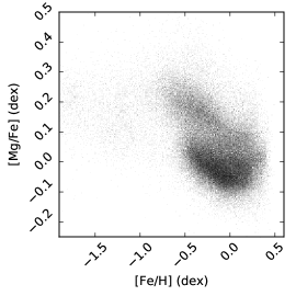
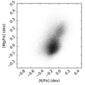
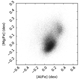
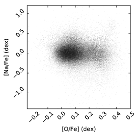
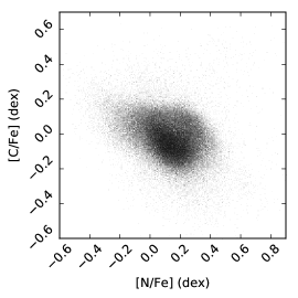
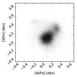
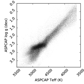
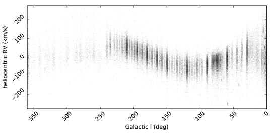
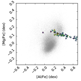
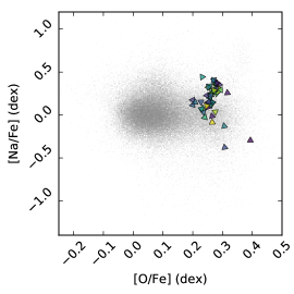
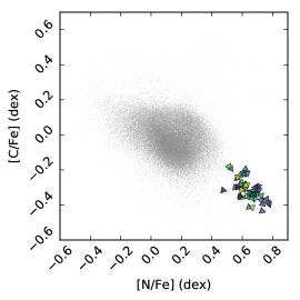
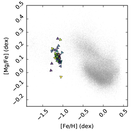
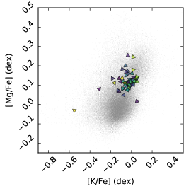
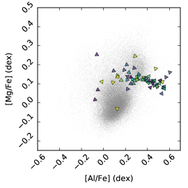
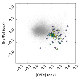
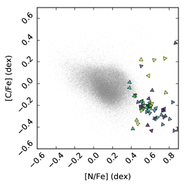
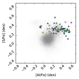
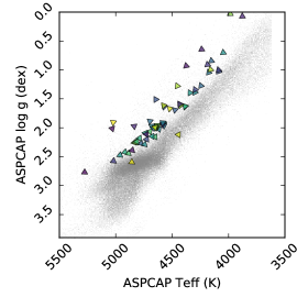
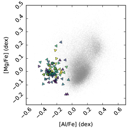
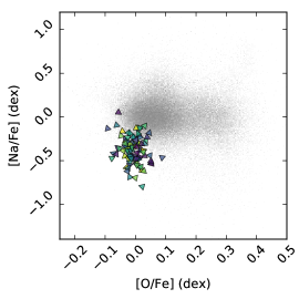
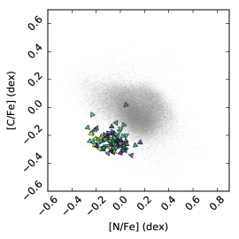
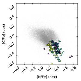
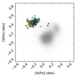
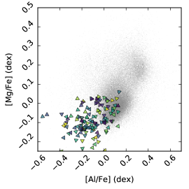
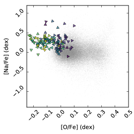
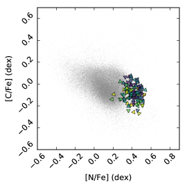
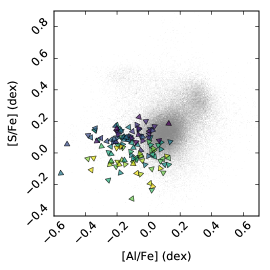
Six two-dimensional projections of the abundance data, plus some other data quantities, are shown in Figure 1. Throughout this work we show two-dimensional abundance projections for only a few elements. The entire sequence of 15-choose-2 combinations is too immense to visualize. The projections shown are ones which have been extensively used in abundance studies of globular clusters and satellite systems. These are typically light element abundances, and our projections include C–N, Na–O, and Mg–Al. Globular clusters famously demonstrate correlations in these elements (for example, Norris & Da Costa, 1995; Carretta et al., 2009, and references therein), thereby making them suitable projections for us to show in verifying and examining any substructure identified by k-means (or any other clustering algorithm).

Section 3 Identifying abundance-space clusters
Although only hints of small-scale clustering in the abundance space are visible in Figure 1, exploration of the data by hand indicates that known clusters do appear in the high-dimensional abundance space as over-densities. In general, the collapse of 15 dimensions down to 2-d projections will hide, smooth, or dilute any structure; there is no guarantee that a highly featured distribution in 15-d will show features in any 2-d projection, let alone axis-aligned, human-selected projections. This encourages us to look for over-densities automatically in the abundance space and see if anything found that way would be over-dense in phase space. The simplest method for clustering points in -dimensional space is the k-means algorithm (see Bishop 2006 for a pedagogical introduction and references to the original literature).
Briefly, the k-means algorithm is the following: Start at some initial guess for the locations of -space cluster centers ( locations in the -dimensional space). Assign each point in the space (each star in our case) to the closest of the centers. Given this assignment of stars to centers, update each center (each of the -space positions) by taking the mean of the locations of the stars assigned to that center. Iterate these steps (assignment of points, followed by taking of means) to convergence. The output of this algorithm is the converged locations of the centers and the assignments of all points to those centers. This algorithm is fast and performs well in practice in problems of this nature; also we are not the first to use the k-means algorithm in abundance space (Gratton et al., 2012).
The k-means algorithm has a number of limitations: One is that must be chosen by hand (or heuristically at best). Here we are only demonstrating a concept; we don’t need to have the best possible clustering. For this reason we simply choose , , and and look at all the results. Also, the k-means algorithm only performs local optimization. At each we perform 32 restarts with different initializations, and preserve the best clustering (best according to the k-means score). Each of the 32 initializations was performed with the scikit-learn standard k-means initialization procedure (Pedregosa et al., 2011).
Another issue with k-means is that it effectively uses metric distances in the -space; it presumes Euclidean isotropy. We choose here to work in the hydrogen-normalized abundance space, the space of [C/H], [N/H], [O/H], [Na/H], [Mg/H], [Al/H], [Si/H], [S/H], [K/H], [Ca/H], [Ti/H], [V/H], [Mn/H], [Fe/H], [Ni/H]. But in addition to this, we re-scale these by approximate typical measurement precisions obtained by The Cannon before running k-means. These scalings were [C/H]/0.041, [N/H]/0.044, [O/H]/0.037, [Na/H]/0.111, [Mg/H]/0.032, [Al/H]/0.055, [Si/H]/0.041, [S/H]/0.054, [K/H]/0.069, [Ca/H]/0.043, [Ti/H]/0.072, [V/H]/0.146, [Mn/H]/0.041, [Fe/H]/0.019, and [Ni/H]/0.034. This scaling makes the space close to isotropic in measurement uncertainty or observational precision. Finally and related, because it looks for clusters compact in metric distance, k-means is more sensitive to clusters that are spherical in the scaled abundance space than clusters of the same density that are elongated in any sense. Importantly we use only abundance-space information, and no positional or velocity information (nor nor nor any targeting or observational meta-data) as input to the clustering algorithm.
Nothing about this algorithm or our choices are particularly tuned or optimized; this is in no sense the algorithm or the method that reveals the best structures. We chose k-means as a simple and straightforward approach to identifying clusters in high dimensional label space, with very few control parameters or decisions required. It is also an algorithm that is well studied in the machine-learning literature, so it has well understood properties. In practice more complex clustering algorithms may perform better than k-means, or even tuning k-means by heuristically setting is likely to improve upon the results here. This Article serves as a proof of concept. Indeed, it is a feature of this work that even the simplest, most generic clustering algorithm returns interesting structures (as shown below). The prospects for Milky Way science only improve as the clustering algorithm improves.
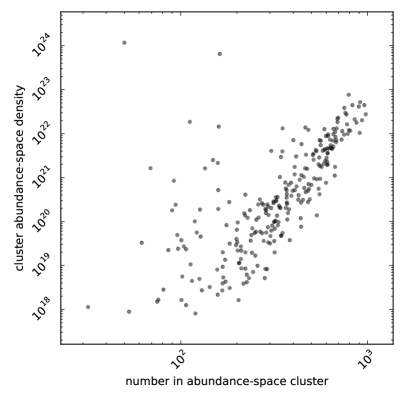
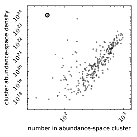
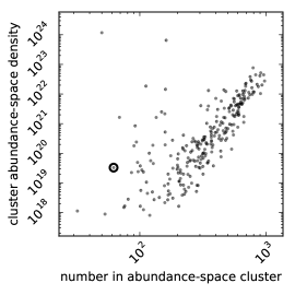
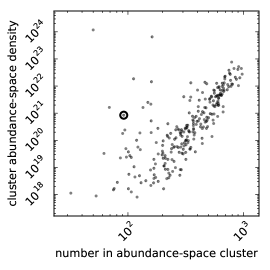
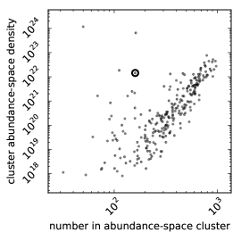
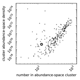
When the k-means results are returned, the empirical variance tensor for the members of each cluster can be constructed. From this, an effective density in the abundance space can be computed as the number of points in the cluster divided by the square-root of the determinant of the tensor. This density was used to rank abundance-space overdensities for visual inspection. In Figure 2 we show the distribution of cluster membership and density for the run of k-means. There is a bulk trend of larger clusters (clusters with more members or higher occupation number) being more dense, but the most interesting k-means densities are those that are more dense than this trend.
Importantly, the k-means algorithm assigns every star to at least one cluster. For this reason, there is no sense in which every “cluster” returned by k-means is a distinct overdensity in abundance space. In what follows, we only consider high-density clusters—clusters that are more dense than average for their occupation number (total membership); these ought to represent true over-densities in abundance space.
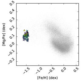
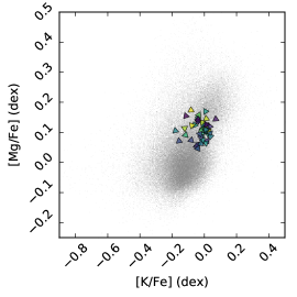
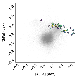
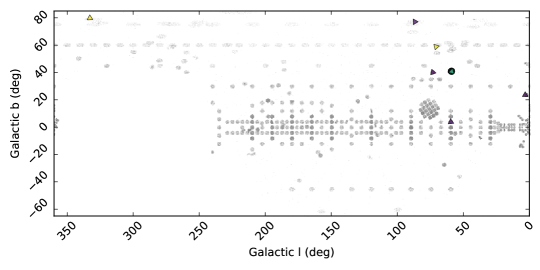
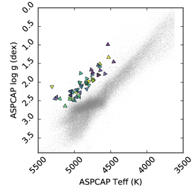
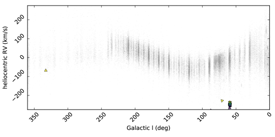
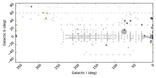
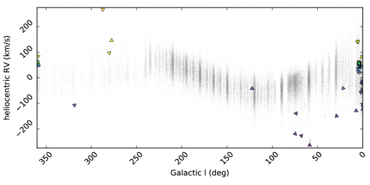
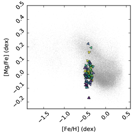
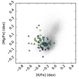
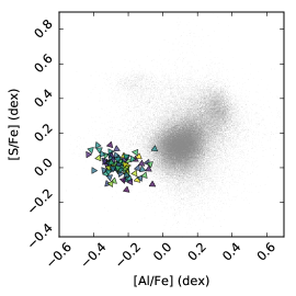
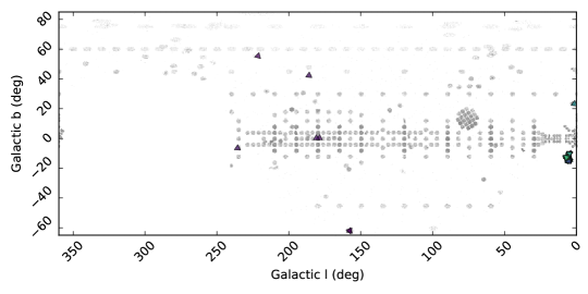
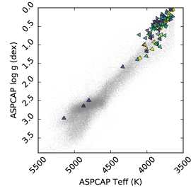
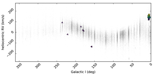
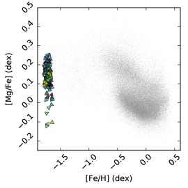
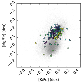
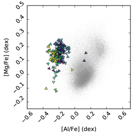
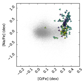
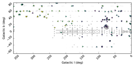
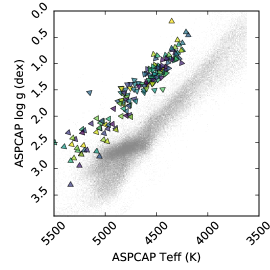
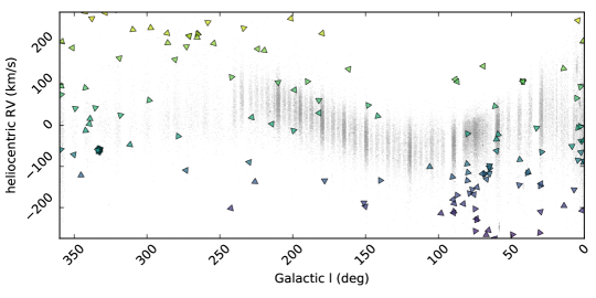
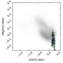
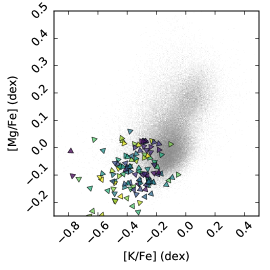
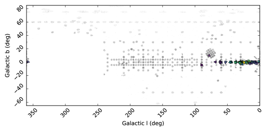
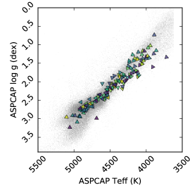
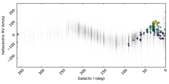
We chose a few interesting cases from the high-density clusters in the run and show them in Figure 3, 4, 5, 6, and 7. The first three of these are dominated by stars in the known clusters M13 and M5, and the Sagittarius stream (we identify overlap with these objects by looking at stellar position and velocity, and, in some cases, APOGEE targeting flags). The fourth is a halo structure with high velocity dispersion and possibly accreted. The fifth is a thin-disk star-formation feature. We will discuss the astrophysical implications of these results in Section 4.
The abundance-space clusters shown in the Figures might not look dense in 2-d projections of the abundance space, but they are very dense in the 15-dimensional space. Indeed, Figure 3 is the densest cluster found in the 15-d space by far. The challenge of this work is to find structure in the high dimensionality space that is not obviously visible in any 2-d projection. Although we have by no means any model of the 15-d space, we do know that the structures shown in the Figures are high in 15-d density, or at least relative to other clusters with the same occupation number.
We have only shown results from the run of k-means. This run was chosen because its densest abundance-space clusters map well onto known stellar clusters. At the densest abundance-space clusters tended to combine multiple known stellar clusters into single, large abundance-space groupings. At k-means tended to split even mono-abundance groups into smaller sub-groups. This is a reminder that k-means has been chosen just for simplicity here; it is by no means matched to the discovery of stellar structures. An important follow-up project is to build a model of abundance space that captures the features expected from stellar populations (and observational uncertainties). Even if we were able to tune k-means in some sense “perfectly”, it would still break up many stellar clusters, since they often show multiple stellar populations and non-linear correlations between element abundances. It is also the case that each of the abundance-space clusters we do show in the Figures includes both star-cluster members and some background contamination, and also is missing some true star-cluster members.
Although we show only three stellar clusters in Figure 3, 4, and 5, many other clusters are visible among our densest abundance-space k-means clusters. These include M15, M92, and M107, among others. We haven’t asked yet whether we detect—as abundance-space overdensities—all of the stellar clusters we expect to find. (Many clusters within the APOGEE data set only contain a few plausible members, thereby complicating any inferences we wish to make about detection completeness using simple k-means.) This Article is simply a demonstration of the chemical-tagging concept; a full investigation of whether we can construct complete catalogs of stellar clusters is beyond our present scope.
Section 4 Discussion
We have demonstrated for the first time that, in a large-scale spectroscopic survey, stars that appear similar in chemical-abundance properties are often associated physically in clusters or other structures. The reverse is well established—that is, that stars that are associated physically in clusters are similar in chemical-abundance properties. That is, although they often show chemical diversity, that chemical diversity is small, and follows well-defined trends or a subspace in abundance space (for example, Gratton et al. 2012; Mészáros et al. 2015; Bovy 2015, and references within those). However, it was not known—prior to this work—whether abundance-space information would be informative enough, or measurable precisely enough to find this structure in surveys dominated by a large mix of stars from different origins and ages. There was good reason to be pessimistic, but plausibly the increased precision obtained here by The Cannon made this possible; even tiny improvements in individual abundances can enormously increase contrast in the high-dimensional abundance space (Ting et al., 2016). We have demonstrated with a straightforward (and in no way optimal) clustering in chemical-abundance space that it is easy to find co-eval stellar structures. Although this is very strong evidence that chemical tagging will work, we have not performed, in any sense, the canonical procedure of looking for features that are consistent with being delta functions in chemical-abundance space (convolved with a measurement noise distribution); we have looked only for over-densities, not delta functions.
One clear result here is that it is easier for the clustering algorithm to find structures at low metallicity than at high metallicity: Some of our low-metallicity features are very compact in phase space, while none of our higher metallicity features are. This probably relates to the much higher background (in abundance space) of unclustered stars at higher metallicities than at low metallicities; in general it is easier to find abundance-space features at the edges of the distribution than in the center (Ting et al., 2016).
What made our success here possible is substantial improvements in precision delivered by The Cannon. We don’t have an absolute measure of the precision of the measurements, but from looking at open and globular clusters, it appears to be on the order of or better than 0.04 dex for the median element in the list of 15. These improvements are discussed in detail in the companion papers (Casey et al., 2016; Ness et al., 2016b) about the abundance measurements. We believe these improvements come from a combination of factors, not limited to (a) improvements in the determination of pseudo-continuum, (b) the use of more spectral range than just unblended element windows (García Pérez et al., 2015), and (c) accurate spectral predictions (The Cannon delivers accurate predictions because it is fit to observed data). Furthermore, because abundance space is high in dimensionality, even small improvements in abundance measurement get taken to a significant power when thinking about information gains.
There are a few points to highlight about the abundance anti-correlations found in globular clusters. First, the detection of these signatures gives confirmation to our analysis: The training (reference) set was not purposefully selected to contain members of any globular or open cluster. However amongst the test set, we recover globular cluster members and their anti-correlations in chemical abundances. That is to say we recover peculiar chemical abundances that are not dominant in our training set, but are expected from previous studies. Secondly, the very presence of complex abundance correlations makes the detection of clusters (by k-means) substantially more difficult. Briefly, the k-means algorithm is most effective for near-normally distributed, isotropic clusters in high-dimensional space. While globular clusters often show distributions of this kind in a few dimensions, they also demonstrate non-linear correlations which would be sub-optimally selected by k-means. For these reasons the fact that (a) The Cannon reports these abundance correlations and (b) k-means (as a simple algorithm without information about expectations in abundance space) does not appear to be severely impacted by these correlations, gives us great hope for more sophisticated approaches. That said, globular cluster members are over-represented in the APOGEE data set, because many of them were specifically targeted for observations for being cluster members (Majewski et al., 2015); that is, globular-cluster structure is over-represented relative to the field in this data set.
The abundances of known clusters that we identify by k-means are in excellent agreement with the literature. For the group shown in Figure 3, which we attribute to M13, we find a mean of [Fe/H]. The mean and spread agree well with other work on this cluster (Kraft et al., 1992; Cohen & Meléndez, 2005; Johnson & Pilachowski, 2012), and compiled catalogs of globular cluster properties (Harris, 1996, accessed 2016). The detailed abundances are also consistent: we find a correlation in [C/Fe] and [N/Fe] abundances (Smith et al., 2005), and their projection in Figure 3 show a spread that reflects deep mixing along the red giant branch (Briley et al., 2004). We find that the light element abundances (most notably Mg–Al) for this cluster are anti-correlated, as expected from other studies (for example, Gratton et al., 2012). However we find a smaller spread in [O/Fe] than reported by others who have looked exclusively at M13 (Johnson & Pilachowski, 2012). As we discuss above, this is expected: k-means is by no means optimal for identifying arbitrary-shaped structures in high-dimensional space, and the first stars that would be assigned to another k-means cluster would be those with the most extreme abundances: low [O/Fe] and high [Na/Fe].
We find a mean metallicity of [Fe/H] for the cluster we associate as M 5 (Figure 4), which agrees well with the [Fe/H] measurement (Koch & McWilliam, 2010), and the value listed in the standard compilation (Harris 1996; accessed 2016). The correlations in light elements—specifically Mg–Al and C–N—also agree well with other studies (Ivans et al., 2001; Mészáros et al., 2015). In particular we find only a weak correlation in the [Na/Fe]–[O/Fe] abundance ratios (Lai et al., 2011). However, when we consider the extent of the literature on M 5, it would suggest that we do not recover the full extent of these correlations: the stars with the highest [Na/Fe], [Mg/Al], and lowest [O/Fe] abundance ratios are not represented in the cluster that we associate as M 5. This is likely a consequence of our (poor) choice of the k-means algorithm, which is most effective for near-circular distributions in the scaled abundance space, and reduced in power for clusters that have polynomial relationships in dimensional space (for example, [Na/Fe]–[O/Fe]). Indeed, abundances for 122 members of M 5 have been reported in APOGEE DR12 data (Mészáros et al. 2015), whereas the cluster we associate as M 5 only contains members, and only covers about half of the extent of [Na/Fe]–[O/Fe] relationship.
All that said, we reiterate a caveat here that we also mentioned in Section 2, which is that at very low metallicity, Na does not show strong lines in any APOGEE spectrum. For this reason, the [Na/Fe] shown for the low-metallicity structures are obtained not by measuring Na lines but rather the lines of elements that correlate strongly with Na at the population level. The true [Na/Fe] may show correlations, variations, or anomalies in the clusters that are not captured by The Cannon working at low metallicity.
The high velocity-dispersion structure seen in Figure 6 stands in stark contrast to the rest of the clusters we have identified. In addition to being highly clustered in 15-dimensions, it is visibly clustered in our 2-d projections. Indeed, it is more clustered in our abundance projections than the young stellar structure in the disk, and comparably so to the other known globular clusters that we have shown here. The disparity between this structure and others presented here is the lack of co-spatial stars. Twelve stars within this cluster are marked as ‘M53’ candidates by APOGEE, but the remaining 145 stars are spread amongst fields throughout the halo.
It is conceivable that this structure, being near the outskirts of the abundance distribution, is somehow concentrated in abundance space by some kind of shrinkage (in the statistical sense) induced by The Cannon’s regression. However, it is a dense feature in abundance space, and is worth following up. If follow-up observations show that the stars have abundances and that are consistent with having origin in a single stellar population or low-metallicity dwarf galaxy, it could represent an accretion event in the Milky Way halo.
The k-means algorithm employed here is by no means optimal, and other clusters we identify are accompanied by a few stars that are not currently co-spatial. Those stars may be unassociated interlopers that have been misclassified, or they may be true cluster members that are now unbound. However in the case of the high-velocity-dispersion structure in Figure 6, the situation is far more extreme. We identify a group of stars with very similar abundances in 15 dimensions that are now spread throughout the Galaxy halo. Because some stars ( percent) are candidate members of the massive globular cluster M53, it provides the tantalizing possibility that these stars may indeed be all members of the same co-natal gas cloud, implying that these stars have been accreted onto the halo from a single globular cluster early in the Milky Way’s formation (as has been hypothesized elsewhere; for example in Martell & Grebel 2010). While speculative, this idea demonstrates the promise of chemical tagging.
The abundance-space group of stars in the disk structure shown in Figure 7 may be associated with a very thin Milky-Way bar component reported previously (Wegg et al., 2015), which is found to exist predominantly toward the end of the bar (at deg). The stars in this structure are metal-rich and have a low [C/N] ratio and are therefore likely young (following the [C/N]–mass relationship; Martig et al. 2016). It is possible that this structure has very low scale height because it is very young and hasn’t experienced dynamical heating or radial migration.
It is worth reiterating here what is written above: There is no sense at all in which Figure 3, 4, 5, 6, and 7 show a representative or complete set of features found in abundance space. These features were hand-chosen to be obviously interesting and interpetable. There are many other things to be found in this data set, and many more effective models to be built of abundance-space structure. The only strong conclusion of this investigation is that chemical tagging can work; the abundance measurements with The Cannon are precise enough and the chemical-abundance space is informative enough.
The APOGEE project shows great promise for these studies, and with the appearance of the companion papers, we will release the chemical-abundance measurements we used here for further study. The future is even brighter, however: APOGEE is expanding to more measured elements, more stars, and all-sky angular coverage with APOGEE2, and GALAH is working towards releasing chemical abundances on a larger set of 29 elements. The APOGEE elements employed in this project include alpha, light proton-capture, odd-Z, and iron peak elements. GALAH will deliver element abundances from all the major nucleosynthetic processes, including light proton capture elements, alpha, odd-Z, iron-peak, as well as neutron-capture elements. Chemical tagging capabilities are expected to grow as the product of the measured nucleosynthetic pathways.
References
- Alam et al. (2015) Alam, S., Albareti, F. D., Allende Prieto, C., et al., 2015, ApJS, 219, 12
- Bishop (2006) Bishop, C. M., 2006, Pattern Recognition and Machine Learning, Springer, New York
- Blanco-Cuaresma et al. (2015) Blanco-Cuaresma, S., Soubiran, C., Heiter, U., et al., 2015, A&A, 577, A47
- Bland-Hawthorn et al. (2010) Bland-Hawthorn, J., Krumholz, M. R., & Freeman, K., 2010, ApJ, 713, 166
- Bovy (2015) Bovy, J., 2015, arXiv:1510.06745
- Briley et al. (2004) Briley, M. M., Cohen, J. G., Stetson, P. B., 2004, AJ, 127, 1579
- Bubar & King (2010) Bubar, E. J., & King, J. R. 2010, AJ, 140, 293
- Carretta et al. (2009) Carretta, E., Bragaglia, A., Gratton, R. G., et al., 2009, A&A, 505, 117
- Casey et al. (2016) Casey, A. R., Hogg, D. W., Ness, M., Rix, H.-W., 2016, in preparation
- Cohen & Meléndez (2005) Cohen, J. G., Meléndez, J., 2005, AJ, 129, 303
- De Silva et al. (2007) De Silva, G. M., Freeman, K. C., Bland-Hawthorn, J., Asplund, M., & Bessell, M. S. 2007, AJ, 133, 694
- De Silva et al. (2015) De Silva, G. M., Freeman, K. C., Bland-Hawthorn, J., et al., 2015, MNRAS, 449, 2604
- Eisenstein et al. (2011) Eisenstein, D. J., Weinberg, D. H., Agol, E., et al., 2011, AJ, 142, 72
- Eggen (1970) Eggen, O. J. 1970, PASP, 82, 99
- Font et al. (2006) Font, A. S., Johnston, K. V., Bullock, J. S., Robertson, B. E., 2006, ApJ, 638, 585
- Freeman & Bland-Hawthorn (2002) Freeman, K., Bland-Hawthorn, J., 2002, ARA&A, 40, 487
- García Pérez et al. (2015) García Pérez, A. E., Allende Prieto, C., Holtzman, J. A., et al., 2015, arXiv:1510.07635
- Gilmore et al. (2012) Gilmore, G., Randich, S., Asplund, M., et al., 2012, The Messenger, 147, 25
- Gratton et al. (2012) Gratton, R. G., Carretta, E., Bragaglia, A., 2012, A&A Rev., 20, 50
- Harris (1996) Harris, W. E., 1996, AJ, 112, 1487
- Helmi et al. (2006) Helmi, A., Navarro, J. F., Nordström, B., Holmberg, J., Abadi, M. G., & Steinmetz, M., 2006, MNRAS, 365, 1309
- Helmi et al. (2014) Helmi, A., Williams, M., Freeman, K. C., Bland-Hawthorn, J., & De Silva, G., 2014, ApJ, 791, 135
- Holtzman et al. (2015) Holtzman, J. A., Shetrone, M., Johnson, J. A., et al., 2015, AJ, 150, 148
- Hunter (2007) Hunter, J. D., 2007, Computing in Science & Engineering, 9, 90
- Ivans et al. (2001) Ivans, I. I., Kraft, R. P., Sneden, C., et al. 2001, AJ, 122, 1438
- Jofré et al. (2015) Jofré, P., Mädler, T., Gilmore, G., et al., 2015, MNRAS, 453, 1428
- Johnson & Pilachowski (2012) Johnson, C. I., Pilachowski, C. A., 2012, ApJ, 754, L38
- Koch & McWilliam (2010) Koch, A., & McWilliam, A. 2010, AJ, 139, 2289
- Kraft et al. (1992) Kraft, R. P., Sneden, C., Langer, G. E., Prosser, C. F., 1992, AJ, 104, 645
- Lai et al. (2011) Lai, D. K., Smith, G. H., Bolte, M., et al. 2011, AJ, 141, 62
- Majewski et al. (2012) Majewski, S. R., Nidever, D. L., Smith, V. V., Damke, G. J., Kunkel, W. E., Patterson, R. J., Bizyaev, D., & Garca P ̵́erez A E,. 2012,ApJ, 747, L37
- Majewski et al. (2015) Majewski, S. R., Schiavon, R. P., Frinchaboy, P. M., et al., 2015, arXiv:1509.05420
- Martell (2015) Martell, S. L., 2015, arXiv:1507.00079
- Martell & Grebel (2010) Martell, S. L., & Grebel, E. K., 2010, A&A, 519, A14
- Martig et al. (2016) Martig, M., Fouesneau, M., Rix, H.-W., et al., 2016, MNRAS, 456, 3655
- Melendez et al. (2014) Meléndez, J., Ramírez, I., Karakas, A. I., et al., 2014, ApJ, 791, 14
- Mészáros et al. (2015) Mészáros, S., Martell, S. L., Shetrone, M., et al., 2015, AJ, 149, 153
- Mitschang et al. (2014) Mitschang, A. W., De Silva, G., Zucker, D. B., et al., 2014, MNRAS, 438, 2753
- Ness et al. (2015) Ness, M., Hogg, D. W., Rix, H.-W., Ho, A. Y. Q., Zasowski, G., 2015, ApJ, 808, 16
- Ness et al. (2016a) Ness, M., Hogg, D. W., Rix, H.-W., et al., 2016a, ApJ, in press (arXiv:1511.08204)
- Ness et al. (2016b) Ness, M., Hogg, D. W., Casey, A. R., Rix, H.-W., 2016b, in preparation
- Norris & Da Costa (1995) Norris, J. E., & Da Costa, G. S. 1995, ApJ, 441, L81
- Pedregosa et al. (2011) Pedregosa, F., Varoquaux, G., Gramfort, A., et al., 2011, Journal of Machine Learning Research, 12, 2825
- Quillen et al. (2015) Quillen, A. C., Anguiano, B., De Silva, G., et al., 2015, MNRAS, 450, 2354
- Roškar et al. (2008) Roškar, R., Debattista, V. P., Quinn, T. R., Stinson, G. S., Wadsley, J., 2008, ApJ, 684, L79
- Smith et al. (2005) Smith, G. H., Briley, M. M., Harbeck, D., 2005, AJ, 129, 1589
- Ting et al. (2016) Ting, Y.-S., Conroy, C., Rix, H.-W., 2016, ApJ, 816, 10
- van der Walt et al. (2011) van der Walt, S., Colbert, S. C., Varoquaux, G., 2011, Computing in Science & Engineering, 13, 22
- Wegg et al. (2015) Wegg, C., Gerhard, O., Portail, M., 2015, MNRAS, 450, 4050