11institutetext: CERN, Geneva, Switzerland

Mathematical and Numerical Methods for Non-linear Beam Dynamics

W. Herr
Abstract

Non-linear effects in accelerator physics are important for both successful operation of accelerators and during the design stage. Since both of these aspects are closely related, they will be treated together in this overview. Some of the most important aspects are well described by methods established in other areas of physics and mathematics. The treatment will be focused on the problems in accelerators used for particle physics experiments. Although the main emphasis will be on accelerator physics issues, some of the aspects of more general interest will be discussed. In particular, we demonstrate that in recent years a framework has been built to handle the complex problems in a consistent form, technically superior and conceptually simpler than the traditional techniques. The need to understand the stability of particle beams has substantially contributed to the development of new techniques and is an important source of examples which can be verified experimentally. Unfortunately, the documentation of these developments is often poor or even unpublished, in many cases only available as lectures or conference proceedings.

0.1 Introduction and motivation

0.1.1 Single-particle dynamics

The concepts developed here are used to describe single-particle transverse dynamics in rings, i.e. circular accelerators or storage rings. In the case of linear betatron motion the theory is rather complete and the standard treatment [1] suffices to describe the dynamics. In parallel with this theory the well-known concepts such as closed orbit and Twiss parameters are introduced and emerge automatically from the Courant–Snyder formalism [1]. The formalism and applications are found in many textbooks (e.g. [2, 3]).

In many new accelerators or storage rings (e.g. the Large Hadron Collider (LHC)) the description of the machine with a linear formalism becomes insufficient and the linear theory must be extended to treat non-linear effects. The stability and confinement of the particles is not given a priori and should rather emerge from the analysis. Non-linear effects are a main source of performance limitations in such machines. Non-linear dynamics has to be used in many applications and the basics are described in the literature [4, 5]. A reliable treatment is required and the progress in recent years allows us to evaluate these effects. A very useful overview and details can be found in [6, 7, 8].

In this article, we restrict the treatment to the beam dynamics in rings, since properties such as stability of particles restrict the form of the tools to describe them. However, many of the concepts (e.g. Lie transformations) can be very beneficial for the analysis of single-pass systems.

0.2 New concepts

The key to the more modern approach shown in this article is to avoid the prejudices about the stability and other properties of the ring. Instead, we must describe the machine in terms of the objects it consists of with all their properties, including the non-linear elements. The analysis will reveal the properties of the particles such as, e.g., stability. In the simplest case, the ring is made of individual machine elements such as magnets which have an existence on their own, i.e. the interaction of a particle with a given element is independent of the motion in the rest of the machine. To successfully study single-particle dynamics, we must be able to describe the action of the machine element on the particle as well as the effect of the machine element in the presence of all other magnets in the ring [9].

0.2.1 Map-based techniques

In the standard approach to single-particle dynamics in rings, the equations of motion are introduced together with an ansatz to solve these equations. In the case of linear motion, this ansatz is known as the Courant–Snyder treatment. However, this treatment must assume that the motion of a particle in the ring is stable and confined. For a non-linear system this is a priori not known and the attempt to find a complete description of the particle motion must fail.

In a more modern approach, we do not attempt to solve such an overall equation but rather consider the fundamental objects of an accelerator, i.e. the machine elements themselves. These elements, e.g. magnets or other beam elements, are the basic building blocks of the machine. All elements have a well-defined action on a particle which can be described independently of other elements or concepts such as closed orbit or β𝛽\beta-functions. Mathematically, they provide a ‘map’ from one face of a building block to the other, i.e. a description of how the particles move inside and between elements. In this context, a map can be anything from linear matrices to high-order integration routines.

The collection of all machine elements makes up the ring and it is the combination of the associated maps which is necessary for the description and analysis of the physical phenomena in the accelerator ring.

The most interesting map is the one which describes the motion once around the machine, the so-called one-turn map (OTM). It contains all necessary information on stability and existence of closed orbit and optical parameters. The reader is assumed to be familiar with this concept in the case of linear beam dynamics [10], where all maps are matrices and the Courant–Snyder analysis of the corresponding OTM produces the desired information such as, e.g., closed orbit or Twiss parameters.

It should therefore be the goal to generalize this concept to non-linear dynamics. The computation of a reliable OTM and the analysis of its properties will provide all relevant information.

Basic concept

Given that the non-linear maps can be rather complex objects, the analysis of the OTM should be separated from the calculation of the map itself.

Using the coordinate vector z=(x,x=x/s,y,y=y/s){\vec{z}}=(x,x^{\prime}={\partial x}/{\partial s},y,y^{\prime}={\partial y}/{\partial s}), the map {{{\cal{M}}}} transforms the coordinates z1(s1)subscript𝑧1subscript𝑠1\vec{z_{1}}(s_{1}) through a magnet M𝑀M at position s1subscript𝑠1{{s_{1}}} to new coordinates z2(s2)subscript𝑧2subscript𝑠2\vec{z_{2}}(s_{2}) at position s2subscript𝑠2{{s_{2}}}:

z2(s2)=(xxyy)s2=(xxyy)s1=z1(s1).subscript𝑧2subscript𝑠2subscript𝑥superscript𝑥𝑦superscript𝑦subscript𝑠2subscript𝑥superscript𝑥𝑦superscript𝑦subscript𝑠1subscript𝑧1subscript𝑠1\displaystyle{{\vec{z_{2}}(s_{2})}}=\left(\begin{array}[]{c}x\\ x^{\prime}\\ y\\ y^{\prime}\\ \end{array}\right)_{{{s_{2}}}}={{\cal{M}}}\circ\left(\begin{array}[]{c}x\\ x^{\prime}\\ y\\ y^{\prime}\\ \end{array}\right)_{{{s_{1}}}}={{\cal{M}}}\circ{{\vec{z_{1}}(s_{1})}}. (9)

The subsequent analysis of the map should reveal the quantities of interest.

0.3 Linear maps

First I shall introduce the simplest form of maps, i.e. linear maps, and generalize afterwards.

0.3.1 Examples for linear maps

As a first example, I consider a drift space of length L𝐿L.

The formal description using the map can be written

(xx)s2=(1L01)(xx)s1.subscript𝑥superscript𝑥subscript𝑠21𝐿01subscript𝑥superscript𝑥subscript𝑠1\displaystyle\left(\begin{array}[]{c}x\\ x^{\prime}\\ \end{array}\right)_{s_{2}}={{\left(\begin{array}[]{cc}1&L\\ 0&1\\ \end{array}\right)}}\circ\left(\begin{array}[]{c}x\\ x^{\prime}\\ \end{array}\right)_{s_{1}}. (16)

As a second example, I show the map (matrix) for a focusing quadrupole of length L𝐿L and strength k𝑘k:

(xx)s2=(cosLk1ksinLkksinLkcosLk)(xx)s1.subscript𝑥superscript𝑥subscript𝑠2𝐿𝑘1𝑘𝐿𝑘𝑘𝐿𝑘𝐿𝑘subscript𝑥superscript𝑥subscript𝑠1\displaystyle\left(\begin{array}[]{c}x\\ x^{\prime}\\ \end{array}\right)_{s_{2}}={{\left(\begin{array}[]{cc}\cos{L\cdot\sqrt{k}}&\frac{1}{\sqrt{k}}\cdot\sin{L\cdot\sqrt{k}}\\ -\sqrt{k}\cdot\sin{L\cdot\sqrt{k}}&\cos{L\cdot\sqrt{k}}\\ \end{array}\right)}}\circ\left(\begin{array}[]{c}x\\ x^{\prime}\\ \end{array}\right)_{s_{1}}. (23)

The map for a quadrupole with short length L𝐿L (i.e. 1Lkmuch-greater-than1𝐿𝑘1\gg L\cdot k) can be approximated by

(xx)s2=(10kL(=1f)1)(xx)s1.subscript𝑥superscript𝑥subscript𝑠210annotated𝑘𝐿absent1𝑓1subscript𝑥superscript𝑥subscript𝑠1\displaystyle\left(\begin{array}[]{c}x\\ x^{\prime}\\ \end{array}\right)_{s_{2}}={{\left(\begin{array}[]{cc}1&0\\ -k\cdot L(=\frac{1}{f})&1\\ \end{array}\right)}}\circ\left(\begin{array}[]{c}x\\ x^{\prime}\\ \end{array}\right)_{s_{1}}. (30)

These are \cal{M}aps, and describe the movement within an element.

0.3.2 OTMs

Starting from a position s0subscript𝑠0s_{0} and applying all maps (for N𝑁N elements) in sequence around a ring with circumference C𝐶C, we get the OTM for the position s0subscript𝑠0s_{0} (for one dimension only):

(xx)s0+C=12N(xx)s0subscript𝑥superscript𝑥subscript𝑠0𝐶subscript1subscript2subscript𝑁subscript𝑥superscript𝑥subscript𝑠0\displaystyle\left(\begin{array}[]{c}x\\ x^{\prime}\\ \end{array}\right)_{{{s_{0}+C}}}={{\cal{M}}_{1}}\circ{{\cal{M}}_{2}}\circ\cdots\circ{{\cal{M}}_{N}}\circ\left(\begin{array}[]{c}x\\ x^{\prime}\\ \end{array}\right)_{{{s_{0}}}} (35)
(xx)s0+C=ring(s0)(xx)s0.subscript𝑥superscript𝑥subscript𝑠0𝐶subscriptringsubscript𝑠0subscript𝑥superscript𝑥subscript𝑠0\displaystyle{{\Longrightarrow}}\leavevmode\nobreak\ \leavevmode\nobreak\ \leavevmode\nobreak\ \left(\begin{array}[]{c}x\\ x^{\prime}\\ \end{array}\right)_{{{s_{0}+C}}}={{\cal{M}}_{\rm ring}(s_{0})}\circ\left(\begin{array}[]{c}x\\ x^{\prime}\\ \end{array}\right)_{{{s_{0}}}}. (40)

After this concatenation, we have obtained a OTM for the whole ring (40). In the simplest case all maps are matrices and the concatenation is just the multiplication of linear matrices. Having obtained this OTM, its analysis will give all relevant information; there is no need for any assumptions. To solve Hill’s equation using the standard ansatz [10], we need several assumptions such as existence of closed orbit and confinement or periodicity. Having derived the map, we have to extract the information needed. To introduce this topic, we first treat a linear OTM, i.e. a matrix.

0.3.3 Linear normal forms

The key to the analysis is that maps (here matrices) can be transformed into (Jordan) normal forms. The original maps and the normal forms are equivalent, but the normal form and the required transformation automatically provide the data we need, such as stability, closed orbit, optical parameters (Q,Q𝑄superscript𝑄Q,Q^{\prime}, Twiss function, etc.), invariants of the motion, resonance analysis, and so on.

Linear normal-form transformation

The basic idea is to make a transformation to get a simpler form for the map.

Assuming that the map 12subscript12{\cal{M}}_{12} propagates the variables from location 111 to location 222, we try to find transformations 𝒜1,𝒜2subscript𝒜1subscript𝒜2{\cal{A}}_{1},{\cal{A}}_{2} such that

𝒜112𝒜21=12.subscript𝒜1subscript12superscriptsubscript𝒜21subscript12\displaystyle{\cal{A}}_{1}{{{\cal{M}}_{12}}}{\cal{A}}_{2}^{-1}={{{\cal{R}}_{12}}}. (41)

The map 12subscript12{\cal{R}}_{12} is a ‘Jordan normal form’ (or at least a very simplified form of the map). For example, 12subscript12{\cal{R}}_{12} becomes a pure rotation, which is a simple and typical normal form. The map 12subscript12{\cal{R}}_{12} describes the same dynamics as 12subscript12{\cal{M}}_{12}, but all coordinates are transformed by 𝒜1subscript𝒜1{\cal{A}}_{1} and 𝒜2subscript𝒜2{\cal{A}}_{2}. The transformations 𝒜1,𝒜2subscript𝒜1subscript𝒜2{\cal{A}}_{1},{\cal{A}}_{2} ‘analyse’ the motion.

Refer to caption
Figure 1: Normal-form transform for a linear OTM (schematic)

We assume that the OTM (here a matrix) (s)𝑠{\cal{M}}(s) at the position s𝑠s is (see e.g. the article on transverse dynamics [10])

(s)=(cos(Δμ)+α(s)sin(Δμ)β(s)sin(Δμ)γ(s)sin(Δμ)cos(Δμ)α(s)sin(Δμ)).𝑠Δ𝜇𝛼𝑠Δ𝜇𝛽𝑠Δ𝜇𝛾𝑠Δ𝜇Δ𝜇𝛼𝑠Δ𝜇\displaystyle{\cal{M}}(s)=\left(\begin{array}[]{cc}\cos(\Delta\mu)+\alpha(s)\sin(\Delta\mu)&\beta(s)\sin(\Delta\mu)\\ -\gamma(s)\sin(\Delta\mu)&\cos(\Delta\mu)-\alpha(s)\sin(\Delta\mu)\\ \end{array}\right). (44)

This matrix describes the motion on a phase-space ellipse. We can rewrite {\cal{M}} such that one part {\cal{R}} becomes a pure rotation (a circle), i.e.

𝒜𝒜1=.𝒜superscript𝒜1\displaystyle{\cal{A}}{\cal{R}}{\cal{A}}^{-1}={\cal{M}}. (45)

Remembering lectures on linear algebra, this transformation is done by the evaluation of the eigenvectors and eigenvalues.

Starting from

M=𝒜(Δμ)𝒜1or(Δμ)=𝒜1M𝒜,formulae-sequence𝑀𝒜Δ𝜇superscript𝒜1orΔ𝜇superscript𝒜1𝑀𝒜\displaystyle{{M}}={\cal{A}}\circ{{{\cal{R}}(\Delta\mu)}}\circ{\cal{A}}^{-1}\quad{\mathrm{or}}\quad{{{\cal{R}}(\Delta\mu)}}={\cal{A}}^{-1}\circ{{M}}\circ{\cal{A}}, (46)

we get for the transformation (𝒜𝒜{\cal{A}}) and the simple form ({\cal{R}})

𝒜=(β(s)0αβ1β(s))and=(cos(Δμ)sin(Δμ)sin(Δμ)cos(Δμ)).formulae-sequence𝒜𝛽𝑠0𝛼𝛽1𝛽𝑠andΔ𝜇Δ𝜇Δ𝜇Δ𝜇\displaystyle{\cal{A}}=\left(\begin{array}[]{cc}\sqrt{\beta(s)}&0\\ -\frac{\alpha}{\sqrt{\beta}}&\frac{1}{\sqrt{\beta(s)}}\\ \end{array}\right)\quad{\mathrm{and}}\quad{\cal{R}}=\left(\begin{array}[]{cc}\cos(\Delta\mu)&\sin(\Delta\mu)\\ -\sin(\Delta\mu)&\cos(\Delta\mu)\\ \end{array}\right). (51)

This is just the Courant–Snyder transformation to get β,α𝛽𝛼\beta,\alpha, etc. and ΔμΔ𝜇\Delta\mu is the tune. That is, the Courant–Snyder analysis is just a normal-form transform of the linear one-turn matrix. This transformation works in more than one dimension using the same formalism. The phase-space ellipse is transformed into a circle, which is the representation of the normal form, i.e. the rotation shown in \Freffig:fig1.
Refer to caption
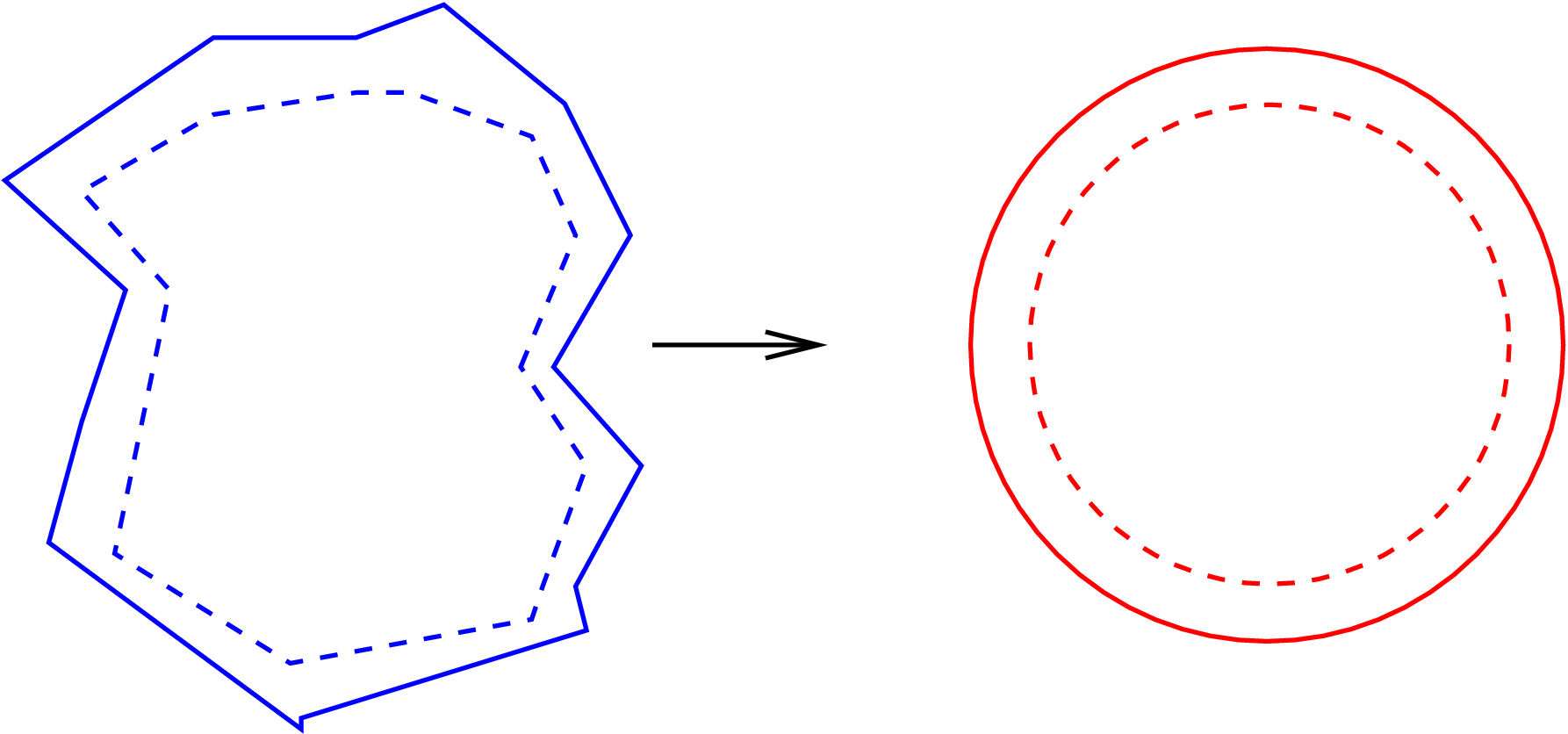
Figure 2: Normal-form transform for a non-linear OTM (schematic)

Compared with the Courant–Snyder analysis, we have the following properties of this method.

  • i)

    The rotation angle (tune for the OTM) ΔμΔ𝜇\Delta\mu is contained in the normalized map, and we have stability for real values of this phase advance ΔμΔ𝜇\Delta\mu.

  • ii)

    Optical functions (β,α(\beta,\alpha, etc.) are in the normalizing map.

  • iii)

    No need to make any assumptions, ansatz or approximation.

In the case of a more complicated OTM (e.g. \Freffig:fig2), the transformation may be more complicated and we have to expect that the rotation angle depends on the amplitude. This is the case for non-linear OTMs, which will be treated in a later section. It has already been mentioned here to introduce the normal-form transformation as a general concept.

Normalized variables

Please note that

(xnxn)=𝒜1(xx)subscript𝑥𝑛subscriptsuperscript𝑥𝑛superscript𝒜1𝑥superscript𝑥\displaystyle\left(\begin{array}[]{c}x_{n}\\ x^{\prime}_{n}\\ \end{array}\right)={{\cal{A}}^{-1}}\circ\left(\begin{array}[]{c}x\\ x^{\prime}\\ \end{array}\right) (56)

in this simple case is just a variable transformation to new, normalized variables.

Action-angle variables

It is common practice to define action-angle variables. Once the particles ‘travel’ on a circle, we can introduce new variables for simplification and easier interpretation of the results.

  • i)

    Radius (say: 2J2𝐽\sqrt{2J}, with J=xn2+xn22𝐽subscriptsuperscript𝑥2𝑛subscriptsuperscript𝑥2𝑛2J=\frac{x^{2}_{n}+x^{\prime 2}_{n}}{2}) is constant (invariant of motion): action J𝐽{{J}}.

  • ii)

    Phase advances by constant amount: angle ΨΨ{{\Psi}}.

The invariant of motion J𝐽J should be the same at all locations in the ring and is separate from the angle ψ𝜓\psi. For the propagation of coordinates around the ring, both are relevant. This separation of the invariant from the angle again becomes important in a later section.

Coupling

The formalism can easily be used to study the case of coupling between the two transverse planes, with the map (in two dimensions)

T=(MnmN),𝑇𝑀𝑛𝑚𝑁\displaystyle T=\left(\begin{array}[]{cc}M&n\\ m&N\\ \end{array}\right), (59)

where M,m,N,n𝑀𝑚𝑁𝑛M,m,N,n are 2×2222\times 2 matrices. In the case of coupling, m0,n0formulae-sequence𝑚0𝑛0m\neq 0,n\neq 0.

We can try to rewrite this using the normal-form algorithms, as before:

T=(MnmN)=VRV1,𝑇𝑀𝑛𝑚𝑁𝑉𝑅superscript𝑉1\displaystyle T=\left(\begin{array}[]{cc}M&n\\ m&N\\ \end{array}\right)=V{{R}}V^{-1}, (62)

with

R=(A00B)andV=(γICCtγI).formulae-sequence𝑅𝐴00𝐵and𝑉𝛾𝐼𝐶superscript𝐶𝑡𝛾𝐼\displaystyle{{R}}=\left(\begin{array}[]{cc}A&0\\ 0&B\\ \end{array}\right)\quad{\mathrm{and}}\quad V=\left(\begin{array}[]{cc}\gamma I&C\\ -C^{t}&\gamma I\\ \end{array}\right). (67)

What have we obtained? The matrix R𝑅R is our simple rotation in two planes and we have in addition:

  • i)

    A𝐴A and B𝐵B are the one-turn matrices for the ‘normal modes’;

  • ii)

    the matrix V𝑉V transforms from the coordinates (x,x,y,y)𝑥superscript𝑥𝑦superscript𝑦(x,x^{\prime},y,y^{\prime}) into the ‘normal-mode’ coordinates (w,w,v,v)𝑤superscript𝑤𝑣superscript𝑣(w,w^{\prime},v,v^{\prime}) via the expression (x,x,y,y)=V(w,w,v,v)𝑥superscript𝑥𝑦superscript𝑦𝑉𝑤superscript𝑤𝑣superscript𝑣(x,x^{\prime},y,y^{\prime})=V(w,w^{\prime},v,v^{\prime});

  • iii)

    the matrix C𝐶C contains the ‘coupling coefficients’.

Multiple turns

Normal forms are extremely useful when a map should be applied k𝑘k times (e.g. k𝑘k turns): the brute-force method would be to multiply the OTM k𝑘k times, which can be very elaborate and expensive in computing time. Instead, we can first make a transformation into a normal form with a rotation matrix R𝑅R, which contains the phase advance per turn μ𝜇\mu. For k𝑘k turns, we have to simply replace the phase advance μ𝜇\mu by the phase advance for k𝑘k turns, which is of course kμ𝑘𝜇k\cdot\mu (68).

Mk(x,x)=ARkA1(x,x)=ARk(X,X).superscript𝑀𝑘𝑥superscript𝑥𝐴superscript𝑅𝑘superscript𝐴1𝑥superscript𝑥𝐴superscript𝑅𝑘𝑋superscript𝑋\displaystyle M^{k}(x,x^{\prime})=AR^{k}\leavevmode\nobreak\ A^{-1}(x,x^{\prime})=AR^{k}(X,X^{\prime}). (68)

Transforming the rotation back into the usual form returns the k𝑘k-turn map.

0.4 Non-linear maps

In this section, I should like to introduce non-linear maps. I shall start with a linear map and than generalize. The effect of a (short) quadrupole depends linearly on amplitude as (rewritten from the matrix form)

z(s2)=(xxyy)s2=(xxyy)s1+(0k1xs10k1ys1).𝑧subscript𝑠2subscript𝑥superscript𝑥𝑦superscript𝑦subscript𝑠2subscript𝑥superscript𝑥𝑦superscript𝑦subscript𝑠10subscript𝑘1subscript𝑥subscript𝑠10subscript𝑘1subscript𝑦subscript𝑠1\displaystyle{\vec{z}(s_{2})}=\left(\begin{array}[]{c}x\\ x^{\prime}\\ y\\ y^{\prime}\\ \end{array}\right)_{s_{2}}=\left(\begin{array}[]{c}x\\ x^{\prime}\\ y\\ y^{\prime}\\ \end{array}\right)_{s_{1}}+\left(\begin{array}[]{c}0\\ k_{1}\cdot{{x_{s_{1}}}}\\ 0\\ k_{1}\cdot{{y_{s_{1}}}}\\ \end{array}\right). (81)

Or, in the already known convention using the matrix 𝐌𝐌{\bf{M}}, z(s2)=𝐌z(s1{\vec{z}(s_{2})}={\bf{M}}\cdot\vec{z}(s_{1}).

0.4.1 Symplecticity

A key concept for the application of maps is a requirement called ‘symplecticity’. In a ring, not all possible maps are allowed. This requires for a matrix {\cal{{{M}}}} that it fulfils the condition

TS=𝒮superscriptT𝑆𝒮\displaystyle{{\cal{{M}}}^{\rm T}\cdot{{S}}\cdot\cal{{{M}}}={{S}}} (82)

with

S=(0100100000010010).𝑆0100100000010010\displaystyle{{S}}=\left(\begin{array}[]{cccc}0&1&0&0\\ -1&0&0&0\\ 0&0&0&1\\ 0&0&-1&0\\ \end{array}\right). (87)

The physical meaning of this requirement is that {\cal{{{M}}}} is area preserving and

limnn=finitedet=1.formulae-sequencesubscript𝑛superscript𝑛finitedet1\displaystyle\lim_{n\rightarrow\infty}{\cal{{{M}}}}^{n}={\mathrm{finite}}\quad\Longrightarrow\quad{\mathrm{det}}\leavevmode\nobreak\ {\cal{{{M}}}}=1. (88)

It should be noted that det=1det1{\mathrm{det}}\leavevmode\nobreak\ {\cal{{{M}}}}=1 is required, but not sufficient, for {\cal{{{M}}}} to be symplectic.

0.4.2 Taylor maps

The effect of a (thin) sextupole with strength k2subscript𝑘2k_{2} is in the form of (81)

z(s2)=(xxyy)s2=(xxyy)s1+(012k2(xs12ys12)0k2(xs1ys1)).𝑧subscript𝑠2subscript𝑥superscript𝑥𝑦superscript𝑦subscript𝑠2subscript𝑥superscript𝑥𝑦superscript𝑦subscript𝑠1012subscript𝑘2superscriptsubscript𝑥subscript𝑠12superscriptsubscript𝑦subscript𝑠120subscript𝑘2subscript𝑥subscript𝑠1subscript𝑦subscript𝑠1\displaystyle{\vec{z}(s_{2})}=\left(\begin{array}[]{c}x\\ x^{\prime}\\ y\\ y^{\prime}\\ \end{array}\right)_{s_{2}}=\left(\begin{array}[]{c}x\\ x^{\prime}\\ y\\ y^{\prime}\\ \end{array}\right)_{s_{1}}+\left(\begin{array}[]{c}0\\ \frac{1}{2}k_{2}\cdot{{(x_{s_{1}}^{2}-y_{s_{1}}^{2})}}\\ 0\\ k_{2}\cdot{{(x_{s_{1}}\cdot y_{s_{1}})}}\\ \end{array}\right). (101)

We can write it now formally as

z(s2)=z(s1).𝑧subscript𝑠2𝑧subscript𝑠1\displaystyle{\vec{z}(s_{2})}={\cal{M}}\circ\vec{z}(s_{1}). (102)

Here \cal{M} is not a matrix but a non-linear map. It cannot be written in linear matrix form. We need something like (for the vector element x𝑥x)

zx(s2)=x(s2)=R11x+R12x+R13y+.+T111x2+T112xxT122x2++T113xy+T114xy++U1111x3+U1112x2x+subscript𝑧𝑥subscript𝑠2𝑥subscript𝑠2subscript𝑅11𝑥subscript𝑅12superscript𝑥subscript𝑅13𝑦missing-subexpressionmissing-subexpressionsubscript𝑇111superscript𝑥2limit-fromsubscript𝑇112𝑥superscript𝑥subscript𝑇122superscript𝑥2missing-subexpressionmissing-subexpressionsubscript𝑇113𝑥𝑦subscript𝑇114𝑥superscript𝑦missing-subexpressionmissing-subexpressionsubscript𝑈1111superscript𝑥3subscript𝑈1112superscript𝑥2superscript𝑥\displaystyle\begin{array}[]{lll}\vec{z_{x}}(s_{2})=x(s_{2})&=&R_{11}\cdot{{x}}+R_{12}\cdot{{x^{\prime}}}+R_{13}\cdot{{y}}+\cdots.\\ &&+T_{111}\cdot{{x^{2}}}+T_{112}\cdot{{xx^{\prime}}}T_{122}\cdot{{x^{\prime 2}}}+\\ &&+T_{113}\cdot{{xy}}+T_{114}\cdot{{xy^{\prime}}}+\cdots\\ &&+U_{1111}\cdot{{x^{3}}}+U_{1112}\cdot{{x^{2}x^{\prime}}}+\cdots\\ \end{array} (107)

and the equivalent for other variables. Please note that x(s2)𝑥subscript𝑠2x(s_{2}) now depends also on the second transverse variable y𝑦y.

Forms of Taylor maps

We can write (107) for j=1,,4𝑗14j=1,\ldots,4:

zj(s2)=k=14Rjkzk(s1)+k=14l=14Tjklzk(s1)zl(s1).subscript𝑧𝑗subscript𝑠2superscriptsubscript𝑘14subscript𝑅𝑗𝑘subscript𝑧𝑘subscript𝑠1superscriptsubscript𝑘14superscriptsubscript𝑙14subscript𝑇𝑗𝑘𝑙subscript𝑧𝑘subscript𝑠1subscript𝑧𝑙subscript𝑠1\displaystyle z_{j}(s_{2})=\sum_{k=1}^{4}{{R_{jk}}}z_{k}(s_{1})+\sum_{k=1}^{4}\sum_{l=1}^{4}{{T_{jkl}}}z_{k}(s_{1})z_{l}(s_{1}). (108)

If this map is truncated after the second order, we call it a second-order map and formally write it as

𝒜2=[R,T].subscript𝒜2𝑅𝑇\displaystyle{{\cal{A}}_{2}}=[{{R}},{{T}}]. (109)

Higher orders can be defined as needed:

𝒜3=[R,T,U][R,T]+k=14l=14m=14Ujklmzk(s1)zl(s1)zm(s1),subscript𝒜3𝑅𝑇𝑈𝑅𝑇superscriptsubscript𝑘14superscriptsubscript𝑙14superscriptsubscript𝑚14subscript𝑈𝑗𝑘𝑙𝑚subscript𝑧𝑘subscript𝑠1subscript𝑧𝑙subscript𝑠1subscript𝑧𝑚subscript𝑠1\displaystyle{{\cal{A}}_{3}}=[R,T,{{U}}]\quad{{\Longrightarrow}}\quad[{{R}},{{T}}]+\sum_{k=1}^{4}\sum_{l=1}^{4}\sum_{m=1}^{4}{{U_{jklm}}}z_{k}(s_{1})z_{l}(s_{1})z_{m}(s_{1}), (110)

which is truncated after the third order.

As an example, the complete second-order map for a (thick) sextupole with length L𝐿L and strength K𝐾K (in two dimensions) is

x2=x1+Lx1K(L24(x12y12)+L36(x1x1y1y1)+L424(x12y12)),x2=x1K(L2(x12y12)+L22(x1x1y1y1)+L36(x12y12)),y2=y1+Ly1+K(L24x1y1+L36(x1y1+y1x1)+L424(x1y1)),y2=y1+K(L2x1y1+L22(x1y1+y1x1)+L36(x1y1)).subscript𝑥2absentsubscript𝑥1𝐿superscriptsubscript𝑥1𝐾superscript𝐿24superscriptsubscript𝑥12superscriptsubscript𝑦12superscript𝐿36subscript𝑥1superscriptsubscript𝑥1subscript𝑦1superscriptsubscript𝑦1superscript𝐿424superscriptsubscript𝑥12superscriptsubscript𝑦12superscriptsubscript𝑥2absentsuperscriptsubscript𝑥1𝐾𝐿2superscriptsubscript𝑥12superscriptsubscript𝑦12superscript𝐿22subscript𝑥1superscriptsubscript𝑥1subscript𝑦1superscriptsubscript𝑦1superscript𝐿36superscriptsubscript𝑥12superscriptsubscript𝑦12subscript𝑦2absentsubscript𝑦1𝐿superscriptsubscript𝑦1𝐾superscript𝐿24subscript𝑥1subscript𝑦1superscript𝐿36subscript𝑥1superscriptsubscript𝑦1subscript𝑦1superscriptsubscript𝑥1superscript𝐿424superscriptsubscript𝑥1superscriptsubscript𝑦1superscriptsubscript𝑦2absentsuperscriptsubscript𝑦1𝐾𝐿2subscript𝑥1subscript𝑦1superscript𝐿22subscript𝑥1superscriptsubscript𝑦1subscript𝑦1superscriptsubscript𝑥1superscript𝐿36superscriptsubscript𝑥1superscriptsubscript𝑦1\displaystyle\begin{array}[]{lll}x_{2}&=x_{1}+Lx_{1}^{\prime}&-K\left(\frac{L^{2}}{4}(x_{1}^{2}-y_{1}^{2})+\frac{L^{3}}{6}(x_{1}x_{1}^{\prime}-y_{1}y_{1}^{\prime})+\frac{L^{4}}{24}(x_{1}^{\prime 2}-y_{1}^{\prime 2})\right),\\ x_{2}^{\prime}&=x_{1}^{\prime}&-K\left(\frac{L}{2}(x_{1}^{2}-y_{1}^{2})+\frac{L^{2}}{2}(x_{1}x_{1}^{\prime}-y_{1}y_{1}^{\prime})+\frac{L^{3}}{6}(x_{1}^{\prime 2}-y_{1}^{\prime 2})\right),\\ y_{2}&=y_{1}+Ly_{1}^{\prime}&+K\left(\frac{L^{2}}{4}x_{1}y_{1}+\frac{L^{3}}{6}(x_{1}y_{1}^{\prime}+y_{1}x_{1}^{\prime})+\frac{L^{4}}{24}(x_{1}^{\prime}y_{1}^{\prime})\right),\\ y_{2}^{\prime}&=y_{1}^{\prime}&+K\left(\frac{L}{2}x_{1}y_{1}+\frac{L^{2}}{2}(x_{1}y_{1}^{\prime}+y_{1}x_{1}^{\prime})+\frac{L^{3}}{6}(x_{1}^{\prime}y_{1}^{\prime})\right).\\ \end{array} (115)

The definition of K𝐾K is not unique; it can differ by some factor, e.g.

(2xt2=kx2versus2xt2=k2x2).formulae-sequencesuperscript2𝑥superscript𝑡2𝑘superscript𝑥2versussuperscript2𝑥superscript𝑡2𝑘2superscript𝑥2\displaystyle\left(\frac{\partial^{2}x}{\partial t^{2}}=k\cdot x^{2}\quad{\mathrm{versus}}\quad\frac{\partial^{2}x}{\partial t^{2}}=\frac{k}{2}\cdot x^{2}\right). (116)

Symplecticity of Taylor maps

We have argued that a vital requirement for maps is the symplecticity. This must hold also for non-linear maps; however:

  • i)

    truncated Taylor expansions are not matrices;

  • ii)

    it is the associated Jacobian matrix 𝒥𝒥{\cal{J}} which must fulfil the symplecticity condition (see (82) and (87)):

    𝒥ik=z2iz1k(e.g.𝒥xy=z2xz1y),\displaystyle{{\cal{J}}_{ik}}=\frac{\partial z^{i}_{2}}{\partial z^{k}_{1}}\quad\left({\mathrm{e.g.}}\ {{\cal{J}}_{xy}}=\frac{\partial z^{x}_{2}}{\partial z^{y}_{1}}\right), (117)

    where 𝒥𝒥{\cal J} must fulfil 𝒥tS𝒥=Ssuperscript𝒥𝑡𝑆𝒥𝑆{\cal J}^{t}\cdot S\cdot{\cal J}=S.

In general, 𝒥ikconstsubscript𝒥𝑖𝑘constabsent{{\cal{{{J}}}}_{ik}}\neq{\rm const}\rightarrow for a truncated Taylor map; this can be difficult to fulfil for all z𝑧z.

As an example, we take the sextupole map (for simplicity in one dimension) [21]

x2=x1+Lx1K(L24x12+L36x1x1+L424x12+𝒪(3)),x2=x1K(L2x12+L22x1x1+L36x12+𝒪(3)).subscript𝑥2absentsubscript𝑥1𝐿superscriptsubscript𝑥1𝐾superscript𝐿24superscriptsubscript𝑥12superscript𝐿36subscript𝑥1superscriptsubscript𝑥1superscript𝐿424superscriptsubscript𝑥12𝒪3superscriptsubscript𝑥2absentsuperscriptsubscript𝑥1𝐾𝐿2superscriptsubscript𝑥12superscript𝐿22subscript𝑥1superscriptsubscript𝑥1superscript𝐿36superscriptsubscript𝑥12𝒪3\displaystyle\begin{array}[]{lll}x_{2}&=x_{1}+Lx_{1}^{\prime}&-K\left(\frac{L^{2}}{4}x_{1}^{2}+\frac{L^{3}}{6}x_{1}x_{1}^{\prime}+\frac{L^{4}}{24}x_{1}^{\prime 2}+{\cal{O}}(3)\right),\\ x_{2}^{\prime}&=x_{1}^{\prime}&-K\left(\frac{L}{2}x_{1}^{2}+\frac{L^{2}}{2}x_{1}x_{1}^{\prime}+\frac{L^{3}}{6}x_{1}^{\prime 2}+{\cal{O}}(3)\right).\\ \end{array} (120)

Then we can compute

𝒥TS𝒥=(01+ΔS1ΔS0)S.superscript𝒥T𝑆𝒥01Δ𝑆1Δ𝑆0𝑆\displaystyle{\cal{J}}^{\rm T}\cdot S\cdot{\cal{J}}=\left(\begin{array}[]{cc}0&1{{+\Delta S}}\\ -1{{-\Delta S}}&0\\ \end{array}\right)\neq S. (123)

We find that 𝒥𝒥{\cal{J}} is non-symplectic with the error

ΔS=K72L4(L2x2+6Lxx+6x2).Δ𝑆𝐾72superscript𝐿4superscript𝐿2superscript𝑥26𝐿𝑥superscript𝑥6superscript𝑥2\displaystyle{{\Delta S}}=\frac{K}{72}L^{4}(L^{2}x^{\prime 2}+6Lxx^{\prime}+6x^{2}). (124)

0.5 Thin elements

From Eq. (124), we may get a hint of how to attack this problem. The error ΔSΔ𝑆\Delta S compared to the fully symplectic map depends on the fourth power of the sextupole length L4superscript𝐿4L^{4}. This can be extended to other elements as well and for short objects the error may be negligible. We can attempt to ‘make’ all elements thin, i.e. short enough to have a negligible non-symplecticity. For this purpose, we define thin elements, i.e. an element with no length, because they avoid problems with symplecticity of non-linear maps such as Taylor maps. The error in equation (124) becomes zero.

0.5.1 Concept of thin elements

Real magnets have a finite length, i.e. they are thick magnets. The field and length are used to compute their effect, i.e. the map; in the simplest case it becomes a matrix (23). In passing, we have already mentioned the equivalent matrix for a quadrupole with zero length (30), since it is often used in analytical calculations. A severe consequence of thick elements is that they are not always linear elements (even not dipoles or quadrupoles). For thick, non-linear magnets a closed solution for maps often does not exist.
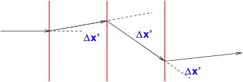
Refer to caption
Figure 3: Movement of a particle through thin elements

The procedure we shall apply to get ‘thin’ magnets is to let the length go to zero, but keep the field integral finite (constant) As consequences, thin dipoles and quadrupoles are linear elements and all thin magnets are much easier to use and automatically symplectic. The movement of a particle through thin elements is shown schematically in \Freffig:fig3. The key is that there is no change of amplitudes x𝑥x and y𝑦y at the element; only the momenta xsuperscript𝑥x^{\prime} and ysuperscript𝑦y^{\prime} receive an amplitude-dependent deflection (kick)

xx+Δxandyy+Δy.formulae-sequencesuperscript𝑥superscript𝑥Δsuperscript𝑥andsuperscript𝑦superscript𝑦Δsuperscript𝑦\displaystyle x^{\prime}\rightarrow x^{\prime}+{{\Delta x^{\prime}}}\quad{\mathrm{and}}\quad y^{\prime}\rightarrow y^{\prime}+{{\Delta y^{\prime}}}. (125)

Modelling a magnet with a finite length by a thin magnet, we have to pay a price and must ask under which conditions this is a good strategy. We should expect that this approximation is valid when the finite length is small or when the length does not matter. The main questions to answer are as follows.

  • i)

    What happens to the accuracy and the implications for the beam dynamics?

  • ii)

    What is the best implementation of thin magnets to minimize the side effects?

We should study these issues with some simple examples and generalize later.

0.5.2 Accuracy of thin elements

We start again with the exact matrix for a thick quadrupole with the strength K𝐾K and the length L𝐿L.

ss+L=(cosLK1KsinLKKsinLKcosLK).subscript𝑠𝑠𝐿𝐿𝐾1𝐾𝐿𝐾𝐾𝐿𝐾𝐿𝐾\displaystyle{\cal{M}}_{s\rightarrow s+L}={{\left(\begin{array}[]{cc}\cos{L\cdot\sqrt{K}}&\frac{1}{\sqrt{K}}\cdot\sin{L\cdot\sqrt{K}}\\ -\sqrt{K}\cdot\sin{L\cdot\sqrt{K}}&\cos{L\cdot\sqrt{K}}\\ \end{array}\right).}} (128)

This matrix describes the motion in a thick quadrupole exactly and we can estimate the errors we make by our approximation. Although this demonstration is done for a quadrupole, the final result is valid for all linear and non-linear elements.

From the exact matrix

ss+L=(cosLK1KsinLKKsinLKcosLK),subscript𝑠𝑠𝐿𝐿𝐾1𝐾𝐿𝐾𝐾𝐿𝐾𝐿𝐾\displaystyle{\cal{M}}_{s\rightarrow s+L}={{\left(\begin{array}[]{cc}\cos{L\cdot\sqrt{K}}&\frac{1}{\sqrt{K}}\cdot\sin{L\cdot\sqrt{K}}\\ -\sqrt{K}\cdot\sin{L\cdot\sqrt{K}}&\cos{L\cdot\sqrt{K}}\\ \end{array}\right),}} (131)

we make a Taylor expansion in ‘small’ length L𝐿L:

L0(1001)+L1(01K0)+L2(K200K2)+superscript𝐿01001superscript𝐿101𝐾0superscript𝐿2𝐾200𝐾2\displaystyle{{L^{0}}}\cdot\left(\begin{array}[]{cc}1&0\\ 0&1\\ \end{array}\right)+{{L^{1}}}\cdot\left(\begin{array}[]{cc}0&1\\ -K&0\\ \end{array}\right)+{{L^{2}}}\cdot\left(\begin{array}[]{cc}-\frac{K}{2}&0\\ 0&-\frac{K}{2}\\ \end{array}\right)+\cdots (138)

and keep up to the first-order term in L𝐿L:

ss+L=L0(1001)+L1(01K0),subscript𝑠𝑠𝐿superscript𝐿01001superscript𝐿101𝐾0\displaystyle{\cal{M}}_{s\rightarrow s+L}={{L^{0}}}\cdot\left(\begin{array}[]{cc}1&0\\ 0&1\\ \end{array}\right)+{{L^{1}}}\cdot\left(\begin{array}[]{cc}0&1\\ -K&0\\ \end{array}\right), (143)
ss+L=(1LKL1)+𝒪(L2).subscript𝑠𝑠𝐿1𝐿𝐾𝐿1𝒪superscript𝐿2\displaystyle{\cal{M}}_{s\rightarrow s+L}={{\left(\begin{array}[]{cc}1&L\\ -K\cdot L&1\\ \end{array}\right)+{\cal{O}}(L^{2})}}. (146)

We make two observations from the approximation (146).

  • i)

    It is precise to first order 𝒪(L1)𝒪superscript𝐿1{\cal{O}}(L^{1}) and the error is to second order 𝒪(L2)𝒪superscript𝐿2{\cal{O}}(L^{2}).

  • ii)

    We have det 11{\cal{M}}\neq 1; therefore, it cannot be symplectic (see 82 and 87).

To ensure the symplecticity, we need to modify the matrix. We can try to add a term in the matrix:

ss+L=(1LKL1)+𝒪(L2)subscript𝑠𝑠𝐿1𝐿𝐾𝐿1𝒪superscript𝐿2\displaystyle{\cal{M}}_{s\rightarrow s+L}={{\left(\begin{array}[]{cc}1&L\\ -K\cdot L&1\\ \end{array}\right)+{{{\cal{O}}(L^{2})}}}} (149)

and we obtain

ss+L=(1LKL1KL2).subscript𝑠𝑠𝐿1𝐿𝐾𝐿1𝐾superscript𝐿2\displaystyle{\cal{M}}_{s\rightarrow s+L}={{\left(\begin{array}[]{cc}1&L\\ -K\cdot L&1{{-KL^{2}}}\\ \end{array}\right)}}. (152)

The matrix (152) is still precise to first order 𝒪(L1)𝒪superscript𝐿1{\cal{O}}(L^{1}) but ‘symplectified’ by adding the term KL2𝐾superscript𝐿2-KL^{2}. The added term is inaccurate to second order (because of L2superscript𝐿2L^{2}) and therefore the order of accuracy is not changed by this modification. This procedure restores the symplecticity, but does not change the level of accuracy.

For the next step, we keep up to the second order in L𝐿L from the Taylor expansion (138):

ss+L=(112KL2LKL112KL2)+𝒪(L3).subscript𝑠𝑠𝐿112𝐾superscript𝐿2𝐿𝐾𝐿112𝐾superscript𝐿2𝒪superscript𝐿3\displaystyle{\cal{M}}_{s\rightarrow s+L}={{\left(\begin{array}[]{cc}1-\frac{1}{2}KL^{2}&L\\ -K\cdot L&1-\frac{1}{2}KL^{2}\\ \end{array}\right)+{{{\cal{O}}(L^{3})}}}}. (155)

It is precise to second order 𝒪(L2)𝒪superscript𝐿2{\cal{O}}(L^{2}) and therefore more accurate than (152), but again not symplectic.

We proceed as before and the symplectification now looks like

ss+L=(112KL2L14KL3KL112KL2)+𝒪(L3).subscript𝑠𝑠𝐿112𝐾superscript𝐿2𝐿14𝐾superscript𝐿3𝐾𝐿112𝐾superscript𝐿2𝒪superscript𝐿3\displaystyle{\cal{M}}_{s\rightarrow s+L}={{\left(\begin{array}[]{cc}1-\frac{1}{2}KL^{2}&L{{-\frac{1}{4}KL^{3}}}\\ -K\cdot L&1-\frac{1}{2}KL^{2}\\ \end{array}\right)+{{{\cal{O}}(L^{3})}}}}. (158)

The accuracy is maintained to second order 𝒪(L2)𝒪superscript𝐿2{\cal{O}}(L^{2}) and it is now fully symplectic.

Physical meaning of the symplectification

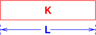
In principle, one could go on with such a scheme, but what is a good strategy? The main issues for using an implementation are accuracy and speed. First, we have a look at the significance of the symplectification, which looks rather arbitrary. Assume a linear element (quadrupole) of length L𝐿L and strength K𝐾K as illustrated in (\Freffig:fig4). A very simple way to apply a thin-lens kick is shown in (\Freffig:fig6). The quadrupole is treated as a drift length of length L𝐿L followed by a thin-length kick with the strength KL𝐾𝐿K\cdot L.

Refer to caption
Figure 4: Schematic picture of a quadrupole with length L𝐿L and strength K𝐾K (convention)
Refer to caption
Figure 5: Schematic picture of a quadrupole with length L𝐿L and a kick with strength K𝐾K at the end of the element

We can compute the full matrix of the drift and the kick and obtain

(10KL1)(1L01)=(1LKL1KL2).10𝐾𝐿11𝐿011𝐿𝐾𝐿1𝐾superscript𝐿2\displaystyle\left(\begin{array}[]{cc}1&0\\ -K\cdot L&1\\ \end{array}\right)\left(\begin{array}[]{cc}1&L\\ 0&1\\ \end{array}\right)=\left(\begin{array}[]{cc}1&L\\ -K\cdot L&1-KL^{2}\\ \end{array}\right). (165)

We find that this resembles the ‘symplectification’ we applied to the truncated map of order 𝒪(L1)𝒪superscript𝐿1{\cal{O}}(L^{1}). Because of the symmetry, we would get the same result when we apply the kick before the drift.

Another option is to apply the thin-lens kick in the centre of the element, as shown in \Freffig:fig7. This time we apply the kick in the centre of the element, preceded and followed by drift spaces of the length L/2𝐿2L/2.

Refer to caption
Figure 6: Schematic picture of a quadrupole with length L𝐿L and a kick with strength K𝐾K in the centre of the element

The multiplication of the three matrices leads us to

ss+L=(112KL2L14KL3KL112KL2)+𝒪(L3).subscript𝑠𝑠𝐿112𝐾superscript𝐿2𝐿14𝐾superscript𝐿3𝐾𝐿112𝐾superscript𝐿2𝒪superscript𝐿3\displaystyle{\cal{M}}_{s\rightarrow s+L}={{\left(\begin{array}[]{cc}1-\frac{1}{2}KL^{2}&L{{-\frac{1}{4}KL^{3}}}\\ -K\cdot L&1-\frac{1}{2}KL^{2}\\ \end{array}\right)+{{{\cal{O}}(L^{3})}}}}. (168)

This is equivalent to the truncated and symplectified map of order 𝒪(L2)𝒪superscript𝐿2{\cal{O}}(L^{2}).

We can summarize the two options as follows.

  • i)

    One kick at the end or entry: error (inaccuracy) is of first order 𝒪(L1)𝒪superscript𝐿1{\cal{O}}(L^{1}).

  • ii)

    One kick in the centre: error (inaccuracy) is of second order 𝒪(L2)𝒪superscript𝐿2{\cal{O}}(L^{2}).

We find that it is very relevant how to apply thin lenses and the aim should be to be precise and fast (and simple to implement, for example in a computer program).

0.5.3 Symplectic integration

We introduce now the concept of symplectic integration and start with simple examples and generalize the concept afterwards. Different integration methods exist which yield symplectic maps and we shall discuss some of them which are relevant for our discussion of applications to accelerators.

Can we do better than in the previous examples?

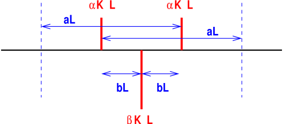
We can try a model with three kicks [18], as shown in \Freffig:fig8. We assume that the kicks (c1, c2, c3) and drift spaces (d1, d2, d3, d4) are variable. We can look for an optimization of these variables to get the best accuracy (i.e. smallest deviation from the exact solution). Since we have only thin lenses, the symplecticity is automatically ensured.

Refer to caption
Figure 7: Symplectic integrator with three thin lenses (schematic)

The results of the optimization of the strengths and the drift spaces between thin kicks are shown in \Freffig:fig9. The optimization of the free parameters gives the values (see \Freffig:fig9): a0.6756𝑎0.6756a\approx 0.6756, b0.1756𝑏0.1756b\approx-0.1756, α1.3512𝛼1.3512\alpha\approx 1.3512, β1.7024𝛽1.7024\beta\approx-1.7024.

Refer to caption
Figure 8: Symplectic integrator with three thin lenses (schematic)

It can easily be shown [18] that using this technique with three kicks, we obtain a 𝒪(4)𝒪4{\cal{O}}(4) integrator. We should expect that more kicks improve the accuracy and as an example a 𝒪(6)𝒪6{\cal{O}}(6) integrator would require nine kicks. This will be shown next.

Yoshida formalism

What we have done is a symplectic integration [18, 19]. From a lower order integration scheme (one kick), we can construct a higher order scheme. Formally (for the formulation of Sk(t)subscript𝑆𝑘𝑡S_{k}(t) see later), we can write: from a second-order scheme (one kick) S2(t)subscript𝑆2𝑡S_{2}(t) we construct a fourth-order scheme (three kicks = 3×1313\times 1 kick) like

S4(t)=S2(x1t)S2(x0t)S2(x1t)subscript𝑆4𝑡subscript𝑆2subscript𝑥1𝑡subscript𝑆2subscript𝑥0𝑡subscript𝑆2subscript𝑥1𝑡\displaystyle S_{4}(t)=S_{2}(x_{1}t)\circ S_{2}(x_{0}t)\circ S_{2}(x_{1}t) (169)

with the coefficients

x0=21/3221/31.7024,x1=1221/31.3512.formulae-sequencesubscript𝑥0superscript2132superscript2131.7024subscript𝑥112superscript2131.3512\displaystyle x_{0}=\frac{-2^{1/3}}{2-2^{1/3}}\approx-1.7024,\quad x_{1}=\frac{1}{2-2^{1/3}}\approx 1.3512. (170)

Equation (169) should be understood symbolically in that we construct a fourth-order integrator from three second-order integrators. As a further example from a fourth order to a sixth order, we have to use

S6(t)=S4(x1t)S4(x0t)S4(x1t).subscript𝑆6𝑡subscript𝑆4subscript𝑥1𝑡subscript𝑆4subscript𝑥0𝑡subscript𝑆4subscript𝑥1𝑡\displaystyle S_{6}(t)=S_{4}(x_{1}t)\circ S_{4}(x_{0}t)\circ S_{4}(x_{1}t). (171)

The interpretation of this construct is that we get three times fourth order with three kicks each; we have the nine-kick, sixth-order integrator mentioned earlier. This is shown schematically in \Freffig:fig10. The three different colours correspond to the three fourth-order integrators, put together into a sixth-order integrator. The sixth-order integrator requires nine kicks and we have three interleaved fourth-order integrators. Going to higher order such as eighth order, we need three interleaved sixth-order integrators, altogether 27 thin lenses. The key is that this can be used as an iterative scheme to go to very high orders and can easily be implemented on a computer. More importantly, the coefficients in (170) are the same in this iterative procedure.
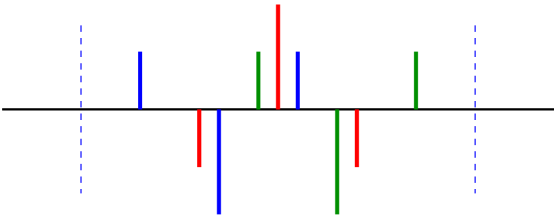
Refer to caption
Figure 9: Symplectic integrator with nine thin lenses (schematic)

As a general formula, we can express this procedure as

Sk+2(t)=Sk(x1t)Sk(x0t)Sk(x1t).subscript𝑆𝑘2𝑡subscript𝑆𝑘subscript𝑥1𝑡subscript𝑆𝑘subscript𝑥0𝑡subscript𝑆𝑘subscript𝑥1𝑡\displaystyle S_{k+2}(t)=S_{k}(x_{1}t)\circ S_{k}(x_{0}t)\circ S_{k}(x_{1}t). (172)

In practice, this means that each kick in the k𝑘kth-order integrator is replaced by a k𝑘kth-order integrator scaled accordingly to obtain a scheme of (k+2)𝑘2(k+2)th order.

We have used a linear map (quadrupole) to demonstrate the integration, but it can be applied to other maps (solenoids, higher-order, non-linear maps). It was shown [18, 19] that this is indeed possible and, most importantly, we get the same integrators. The proof and the systematic extension can be done in the form of Lie operators. It can be proven that this scheme gives the theoretically best possible accuracy for a given number of thin elements.

Integration of non-linear elements

We demonstrate now this formalism for non-linear elements. Let us assume a general case:

x′′superscript𝑥′′\displaystyle x^{\prime\prime} =\displaystyle= f(x).𝑓𝑥\displaystyle f(x). (173)

The disadvantage of a kick (173) is that usually a closed solution through the element does not exist and an integration is necessary.

The advantage of non-linear elements is that they are usually thin (at least thinner than dipoles or quadrupoles). As examples, we give the lengths of typical LHC magnets.

  • i)

    Dipoles: \approx 14.3 m.

  • ii)

    Quadrupoles: \approx 2–5 m.

  • iii)

    Sextupoles, octupoles: \approx 0.30 m.

We can hope to obtain a good approximation for elements with small lengths. To get an estimate, we try our simplest 𝒪(2)𝒪2{\cal{O}}(2) thin-lens approximation first. Therefore, we represent the non-linear element as a thin-lens kick (173) with drift spaces of L/2𝐿2L/2 before and after the kick.

Accuracy of thin lenses: our 𝒪(2)𝒪2{\cal{O}}(2) model

Assuming the general case for a non-linear kick ΔxΔsuperscript𝑥\Delta x^{\prime},

x′′superscript𝑥′′\displaystyle x^{\prime\prime} =\displaystyle= f(x)(=Δx),annotated𝑓𝑥absentΔsuperscript𝑥\displaystyle f(x)\quad(={{\Delta x^{\prime}}}), (174)

we follow the three steps:

Step 1.(xx)s1+L/2=(1L201)(xx)s1;\displaystyle\mathrm{Step\leavevmode\nobreak\ 1.}\quad\left(\begin{array}[]{c}x\\ x^{\prime}\\ \end{array}\right)_{s_{1}+L/2}={{\left(\begin{array}[]{cc}1&\frac{L}{2}\\ 0&1\\ \end{array}\right)}}\circ\left(\begin{array}[]{c}x\\ x^{\prime}\\ \end{array}\right)_{s_{1}}; (181)
Step 2.(xx)s1+L/2=(xx+Δx)s1+L/2;\displaystyle\mathrm{Step\leavevmode\nobreak\ 2.}\quad\left(\begin{array}[]{c}x\\ x^{\prime}\\ \end{array}\right)_{s_{1}+L/2}={{\left(\begin{array}[]{c}x\\ x^{\prime}+{{\Delta x^{\prime}}}\\ \end{array}\right)_{s_{1}+L/2}}}; (186)
Step 3.(xx)s1+L=(1L201)(xx)s1+L/2.\displaystyle\mathrm{Step\leavevmode\nobreak\ 3.}\quad\left(\begin{array}[]{c}x\\ x^{\prime}\\ \end{array}\right)_{s_{1}+L}={{\left(\begin{array}[]{cc}1&\frac{L}{2}\\ 0&1\\ \end{array}\right)}}\circ\left(\begin{array}[]{c}x\\ x^{\prime}\\ \end{array}\right)_{s_{1}+L/2}. (193)

Using this thin-lens approximation (𝒪(2)𝒪2{\cal{O}}(2)) gives us for the map

x(L)superscript𝑥𝐿\displaystyle x^{\prime}(L) \displaystyle\approx x0+Lf(x0+L2x0),subscriptsuperscript𝑥0𝐿𝑓subscript𝑥0𝐿2subscriptsuperscript𝑥0\displaystyle x^{\prime}_{0}+Lf(x_{0}+\frac{L}{2}x^{\prime}_{0}),
x(L)𝑥𝐿\displaystyle x(L) \displaystyle\approx x0+L2(x0+x(L)).subscript𝑥0𝐿2subscriptsuperscript𝑥0superscript𝑥𝐿\displaystyle x_{0}+\frac{L}{2}(x^{\prime}_{0}+x^{\prime}(L)). (194)

Here we write x0subscript𝑥0x_{0} and x0subscriptsuperscript𝑥0x^{\prime}_{0} for the coordinates and angles at the entry of the element. The result (194) corresponds to the well-known ‘leap-frog’ algorithm/integration, schematically shown in \Freffig:fig11. It is symplectic and time reversible.
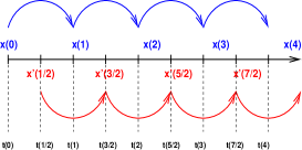
Refer to caption
Refer to caption
Figure 10: Schematic representation of a ‘leap-frog’ integration scheme

For any x′′=f(x,x,t)superscript𝑥′′𝑓𝑥superscript𝑥𝑡x^{\prime\prime}=f(x,x^{\prime},t), we can solve it using

xi+3/2subscriptsuperscript𝑥𝑖32\displaystyle x^{\prime}_{i+3/2} \displaystyle\approx xi+1/2+f(xi+1)Δt,subscriptsuperscript𝑥𝑖12𝑓subscript𝑥𝑖1Δ𝑡\displaystyle x^{\prime}_{i+1/2}+f(x_{i+1})\Delta t,
xi+1subscript𝑥𝑖1\displaystyle x_{i+1} \displaystyle\approx xi+xi+1/2Δt,subscript𝑥𝑖subscriptsuperscript𝑥𝑖12Δ𝑡\displaystyle x_{i}+x^{\prime}_{i+1/2}\Delta t, (195)

which is what is known as a ‘leap-frog’ integration.

Accuracy of the ‘leap-frog’ algorithm/integration

The (exact) Taylor expansion gives

x(L)𝑥𝐿\displaystyle x(L) =\displaystyle= x0+x0L+12f(x0)L2+16x0f(x0)L3+;subscript𝑥0subscriptsuperscript𝑥0𝐿12𝑓subscript𝑥0superscript𝐿216subscriptsuperscript𝑥0superscript𝑓subscript𝑥0superscript𝐿3\displaystyle x_{0}+x^{\prime}_{0}L+\frac{1}{2}f(x_{0})L^{2}+{{\frac{1}{6}}}x^{\prime}_{0}f^{\prime}(x_{0})L^{3}+\cdots; (196)

the (approximate) ‘leap-frog’ algorithm (195) gives

x(L)𝑥𝐿\displaystyle x(L) =\displaystyle= x0+x0L+12f(x0)L2+14x0f(x0)L3+.subscript𝑥0subscriptsuperscript𝑥0𝐿12𝑓subscript𝑥0superscript𝐿214subscriptsuperscript𝑥0superscript𝑓subscript𝑥0superscript𝐿3\displaystyle x_{0}+x^{\prime}_{0}L+\frac{1}{2}f(x_{0})L^{2}+{{\frac{1}{4}}}x^{\prime}_{0}f^{\prime}(x_{0})L^{3}+\cdots. (197)

The two methods differ from L3superscript𝐿3L^{3} onwards and we have an integrator of order 𝒪(L3)𝒪superscript𝐿3{\cal{O}}(L^{3}). This had to be expected since we know from previous considerations that this type of splitting gives such an accuracy. For small L𝐿L, this method is acceptable and symplectic.

As an application, we assume a (one-dimensional) sextupole with (definition of k𝑘k not unique)

x′′superscript𝑥′′\displaystyle x^{\prime\prime} =\displaystyle= kx2=f(x);𝑘superscript𝑥2𝑓𝑥\displaystyle k\cdot x^{2}=f(x); (198)

using the thin-lens approximation using (194) gives

x(L)𝑥𝐿\displaystyle x(L) =\displaystyle= x0+x0L+12kx02L2+12kx0x0L3+18kx02L4,subscript𝑥0subscriptsuperscript𝑥0𝐿12𝑘subscriptsuperscript𝑥20superscript𝐿212𝑘subscript𝑥0subscriptsuperscript𝑥0superscript𝐿318𝑘subscriptsuperscript𝑥20superscript𝐿4\displaystyle x_{0}+x^{\prime}_{0}L+\frac{1}{2}kx^{2}_{0}L^{2}+\frac{1}{2}kx_{0}x^{\prime}_{0}L^{3}+\frac{1}{8}kx^{\prime 2}_{0}L^{4},
x(L)superscript𝑥𝐿\displaystyle x^{\prime}(L) =\displaystyle= x0+kx02L+kx0x0L2+14kx02L3.subscriptsuperscript𝑥0𝑘subscriptsuperscript𝑥20𝐿𝑘subscript𝑥0subscriptsuperscript𝑥0superscript𝐿214𝑘subscriptsuperscript𝑥20superscript𝐿3\displaystyle x^{\prime}_{0}+kx^{2}_{0}L+kx_{0}x^{\prime}_{0}L^{2}+\frac{1}{4}kx^{\prime 2}_{0}L^{3}. (199)

This is the map for a thick sextupole of length L𝐿L in thin-lens approximation, accurate to 𝒪(L2)𝒪superscript𝐿2{\cal{O}}(L^{2}).

0.6 Hamiltonian formalism

In this section, we introduce the Hamiltonian formalism for the classical motion of a particle [20]. We describe the motion of a system by a function L𝐿L:

L(q1,,qn,q1˙,,qn˙,t),𝐿subscript𝑞1subscript𝑞𝑛˙subscript𝑞1˙subscript𝑞𝑛𝑡\displaystyle L(q_{1},\ldots,q_{n},\dot{q_{1}},\ldots,\dot{q_{n}},t), (200)

where (q1,,qnsubscript𝑞1subscript𝑞𝑛q_{1},\ldots,q_{n}) are generalized coordinates and (q1˙,,qn˙˙subscript𝑞1˙subscript𝑞𝑛\dot{q_{1}},\ldots,\dot{q_{n}}) are generalized velocities. For the introduction of the concepts, we use q𝑞q for the coordinate, since it is commonly used in the literature [20]. The function L𝐿L defines the Lagrange function and the integral

I=L(qi,qi˙,t)dt𝐼𝐿subscript𝑞𝑖˙subscript𝑞𝑖𝑡differential-d𝑡\displaystyle I=\int L(q_{i},\dot{q_{i}},t)\,{\mathrm{d}}t (201)

defines the action. Without proof or derivation, we quote [20]

L=TV,𝐿𝑇𝑉\displaystyle L=T-V, (202)

where T𝑇T is the kinetic energy and V𝑉V the potential energy.

Refer to caption
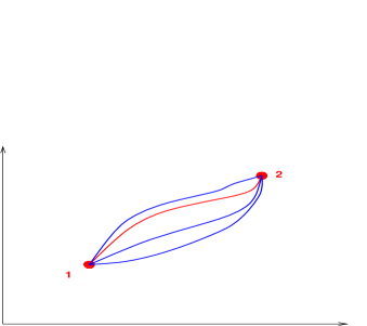
Figure 11: Schematic of the Hamiltonian principle. Different paths and path with minimum action

The Hamiltonian principle states that a system moves such that the action I𝐼I becomes an extremum when different paths are possible. This is schematically shown in \Freffig:fig12. The action becomes a minimum for the red path. Such concepts are known from other applications such as optics or quantum mechanics using Feynman path integrals.

Without proof, the action

I=12L(qi,qi˙,t)dt=extremum𝐼superscriptsubscript12𝐿subscript𝑞𝑖˙subscript𝑞𝑖𝑡differential-d𝑡extremum\displaystyle I=\int_{1}^{2}L(q_{i},\dot{q_{i}},t)\,{\mathrm{d}}t=\mathrm{extremum} (203)

becomes an extremum (minimum) when the Lagrange function fulfils the relation [20]

ddtLqi˙Lqi=0,dd𝑡𝐿˙subscript𝑞𝑖𝐿subscript𝑞𝑖0\displaystyle\frac{{\rm d}}{{\rm d}t}\frac{\partial L}{\partial\dot{q_{i}}}-\frac{\partial L}{\partial q_{i}}=0, (204)

which is usually called the Euler–Lagrange equation.

0.6.1 From the Lagrangian to the Hamiltonian

The Lagrangian L(q1,,qn,q1˙,,qn˙,t)𝐿subscript𝑞1subscript𝑞𝑛˙subscript𝑞1˙subscript𝑞𝑛𝑡L(q_{1},\ldots,q_{n},\dot{q_{1}},\ldots,\dot{q_{n}},t) in generalized coordinates and velocities provides (n𝑛n) second-order differential equations. We can try to get first-order differential equations (which are always solvable) and generalized momenta instead of velocities. This leads us to the Hamiltonian function and the Hamiltonian formalism. The main differences are as follows.

  • i)

    Lagrangian:

    • a)

      n𝑛n second-order equations;

    • b)

      n𝑛n-dimensional coordinate space.

  • ii)

    Hamiltonian:

    • a)

      2n2𝑛2n first-order equations;

    • b)

      2n2𝑛2n-dimensional phase space.

Corresponding (so-called conjugate) momenta pjsubscript𝑝𝑗p_{j} are

pj=Lqj˙.subscript𝑝𝑗𝐿˙subscript𝑞𝑗\displaystyle p_{j}=\frac{\partial L}{\partial\dot{q_{j}}}. (205)

Once we know what the canonical momenta pisubscript𝑝𝑖p_{i} are, the Hamiltonian is a transformation of the Lagrangian:

H(qj,pj,t)=iqi˙piL(qj,qj˙,t).𝐻subscript𝑞𝑗subscript𝑝𝑗𝑡subscript𝑖˙subscript𝑞𝑖subscript𝑝𝑖𝐿subscript𝑞𝑗˙subscript𝑞𝑗𝑡\displaystyle H(q_{j},{{p_{j}}},t)=\sum_{i}{\dot{q_{i}}}{{p_{i}}}-L(q_{j},\dot{q_{j}},t). (206)

Without proof or derivation, we quote [20]

H=T+V,𝐻𝑇𝑉\displaystyle H=T+V, (207)

where T𝑇T is the kinetic energy and V𝑉V the potential energy.

From the Hamiltonian principle, we obtain two first-order equations of motion:

Hqj=pj˙=dpjdt,Hpj=qj˙=dqjdt.formulae-sequence𝐻subscript𝑞𝑗˙subscript𝑝𝑗dsubscript𝑝𝑗d𝑡𝐻subscript𝑝𝑗˙subscript𝑞𝑗dsubscript𝑞𝑗d𝑡\displaystyle\frac{\partial H}{\partial q_{j}}=-\dot{p_{j}}=-\frac{{\rm d}p_{j}}{{\rm d}t},\quad\frac{\partial H}{\partial p_{j}}=\dot{q_{j}}=\frac{{\rm d}q_{j}}{{\rm d}t}. (208)

The key difference to the Lagrangian is that the canonical momenta can be considered as independent variables (contrary to velocities of the coordinates) and are on equal footing with the coordinates. They form a separate set of variables and their time development is treated separately (208).

0.6.2 Hamiltonian of electromagnetic elements in accelerators

For the Hamiltonian of a (relativistic) particle in an electromagnetic field, we have (using from now on the more familiar variable x𝑥x as the coordinate)

(x,p,t)=c(peA(x,t))2+m02c2+eΦ(x,t),𝑥𝑝𝑡𝑐superscript𝑝𝑒𝐴𝑥𝑡2superscriptsubscript𝑚02superscript𝑐2𝑒Φ𝑥𝑡\displaystyle{\cal{H}}(\vec{x},\vec{p},t)=c\sqrt{(\vec{p}-e\vec{A}(\vec{x},t))^{2}+m_{0}^{2}c^{2}}+e\Phi(\vec{x},t), (209)

where A(x,t)𝐴𝑥𝑡\vec{A}(\vec{x},t), Φ(x,t)Φ𝑥𝑡\Phi(\vec{x},t) are the vector and scalar potentials. Using canonical variables and the design path length s𝑠s as independent variable (bending in x𝑥x-plane),

=(1+xρ)(1+δ)2px2py2+xρ+x22ρ2As(x,y)B0ρ,1𝑥𝜌superscript1𝛿2superscriptsubscript𝑝𝑥2superscriptsubscript𝑝𝑦2𝑥𝜌superscript𝑥22superscript𝜌2subscript𝐴𝑠𝑥𝑦subscript𝐵0𝜌\displaystyle{\cal{H}}=-\left(1+\frac{x}{\rho}\right)\cdot\sqrt{(1+\delta)^{2}-p_{x}^{2}-p_{y}^{2}}+\frac{x}{\rho}+\frac{x^{2}}{2\rho^{2}}-\frac{A_{s}(x,y)}{B_{0}\rho}, (210)

where δ=(pp0)/p𝛿𝑝subscript𝑝0𝑝\delta=(p-p_{0})/p is the relative momentum deviation and As(x,y)subscript𝐴𝑠𝑥𝑦A_{s}(x,y) the longitudinal component of the vector potential.

In general, the magnetic fields can be described with the multipole expansion

By+iBx=n=1(bn+ian)(x+iy)n1subscript𝐵𝑦isubscript𝐵𝑥subscript𝑛1subscript𝑏𝑛isubscript𝑎𝑛superscript𝑥i𝑦𝑛1\displaystyle B_{y}+{\rm i}B_{x}=\sum_{n=1}(b_{n}+{\rm i}a_{n})(x+{\rm i}y)^{n-1} (211)

and, since B=×A𝐵𝐴\vec{B}=\nabla\times\vec{A} for the vector potential A𝐴\vec{A},

As(x,y)=n=11n[(bn+ian)(x+iy)n].subscript𝐴𝑠𝑥𝑦subscript𝑛11𝑛delimited-[]subscript𝑏𝑛isubscript𝑎𝑛superscript𝑥i𝑦𝑛\displaystyle A_{s}(x,y)=\sum_{n=1}\frac{1}{n}[(b_{n}+{\rm i}a_{n})(x+{\rm i}y)^{n}]. (212)

Here n=1𝑛1n=1 refers to dipolar fields (not always the case and different conventions exist). For a large machine (xρmuch-less-than𝑥𝜌x\ll\rho), we expand the root and sort the variables to get

=px2+py22(1+δ)kinematicxδρdispersive+x22ρ2focusingdipole+k12(x2y2)quadrupole+k26(x33xy2)sextupolesuperscriptsuperscriptsubscript𝑝𝑥2superscriptsubscript𝑝𝑦221𝛿𝑘𝑖𝑛𝑒𝑚𝑎𝑡𝑖𝑐superscriptsubscript𝑥𝛿𝜌𝑑𝑖𝑠𝑝𝑒𝑟𝑠𝑖𝑣𝑒subscriptsuperscript𝑥22superscript𝜌2𝑓𝑜𝑐𝑢𝑠𝑖𝑛𝑔𝑑𝑖𝑝𝑜𝑙𝑒superscriptsubscript𝑘12superscript𝑥2superscript𝑦2𝑞𝑢𝑎𝑑𝑟𝑢𝑝𝑜𝑙𝑒superscriptsubscript𝑘26superscript𝑥33𝑥superscript𝑦2𝑠𝑒𝑥𝑡𝑢𝑝𝑜𝑙𝑒\displaystyle{\cal{H}}=\overbrace{\frac{p_{x}^{2}+p_{y}^{2}}{2(1+\delta)}}^{kinematic}-\overbrace{\underbrace{\frac{x\delta}{\rho}}_{dispersive}+\underbrace{\frac{x^{2}}{2\rho^{2}}}_{focusing}}^{dipole}+\overbrace{\frac{k_{1}}{2}(x^{2}-y^{2})}^{quadrupole}+\overbrace{\frac{k_{2}}{6}(x^{3}-3xy^{2})}^{sextupole} (213)
(using MAD convention:kn=1BρnByxn).using MAD convention:subscript𝑘𝑛1𝐵𝜌superscript𝑛subscript𝐵𝑦superscript𝑥𝑛\displaystyle\left(\mbox{using\leavevmode\nobreak\ MAD\leavevmode\nobreak\ convention:}\quad k_{n}=\frac{1}{B\rho}\frac{\partial^{n}B_{y}}{\partial x^{n}}\right). (214)

We can see the contribution to the different multipole fields. The Hamiltonian describes exactly the motion of a particle through a magnet. This is our basis to extend the linear to a non-linear formalism.

But how do we apply it to an accelerator? A standard method used in the past was to derive a grandiose Hamiltonian for the whole ring. In that case one views the machine elements (magnets) as a localized fluctuation in the variable s𝑠s, requiring a large set of Fourier modes. In this traditional treatment one tries to find a global description of the entire ring to derive the aspects of beam dynamics of interest. This goal is usually doomed to fail for complex systems, in particular with localized strong and non-linear objects such as beam–beam interactions in a collider. It is the humble opinion of the author that such an approach does not reach beyond (doubtful) pedagogical purposes.

Instead, I shall treat individual magnets as objects having an existence on their own. The magnets are treated as local𝑙𝑜𝑐𝑎𝑙local objects where we can compute the map for the magnet. In a global view it is not possible to have an idea of the effect of a single magnet (e.g. a quadrupole) unless the Twiss parameters at the locations of the magnets are known. This requires a priori knowledge of the OTM.

This ‘local’ approach is clearly influenced by the computer simulation of accelerators where conceptually all elements are treated as separate objects, which are described (and used) independently of ‘global’ concepts such as closed orbits, beta functions etc. With this treatment the properties of the ring such as stability and optical functions will arise naturally, as demonstrated in the simple introduction to linear normal forms. The description of machine elements can be easily achieved by defining the maps through their individual Hamiltonians. This allows naturally the treatment of non-linear elements and in connection to simulations it translates itself into the ‘object-oriented’ approach in computer science. Concepts built on this approach are described in detail in [6].

In the next step we proceed to present the necessary tools.

0.6.3 Poisson brackets

We introduce a Poisson bracket for a differential operator [20]:

[f,g]=i=1n(fxigpifpigxi).𝑓𝑔superscriptsubscript𝑖1𝑛𝑓subscript𝑥𝑖𝑔subscript𝑝𝑖𝑓subscript𝑝𝑖𝑔subscript𝑥𝑖\displaystyle[f,g]=\sum_{i=1}^{n}\left(\frac{\partial f}{\partial x_{i}}\frac{\partial g}{\partial p_{i}}-\frac{\partial f}{\partial p_{i}}\frac{\partial g}{\partial x_{i}}\right). (215)

Here the variables xi,pisubscript𝑥𝑖subscript𝑝𝑖x_{i},p_{i} are canonical variables; f𝑓f and g𝑔g are any functions of xisubscript𝑥𝑖x_{i} and pisubscript𝑝𝑖p_{i}.

We can now write (using the Hamiltonian H𝐻H for the function g𝑔g in (215)

f(xi,pi)=xi[xi,H]=Hpi=dxidt,\displaystyle f(x_{i},p_{i})=x_{i}\Rightarrow\leavevmode\nobreak\ \leavevmode\nobreak\ [x_{i},H]=\frac{\partial H}{\partial p_{i}}=\frac{{\rm d}x_{i}}{{\rm d}t}, (216)
f(xi,pi)=pi[pi,H]=Hxi=dpidt.\displaystyle f(x_{i},p_{i})=p_{i}\Rightarrow\leavevmode\nobreak\ \leavevmode\nobreak\ [p_{i},H]=-\frac{\partial H}{\partial x_{i}}=\frac{{\rm d}p_{i}}{{\rm d}t}. (217)

Therefore, Poisson brackets encode Hamiltons’s equations [20]. In general, the Poisson bracket [f,H]𝑓𝐻[f,H] describes the time evolution of the system (i.e. the function f𝑓f). It is a special case of

dfdt=[f,H]+ft.d𝑓d𝑡𝑓𝐻𝑓𝑡\displaystyle\frac{{\rm d}f}{{\rm d}t}=[f,H]+\frac{\partial f}{\partial t}. (218)

If H𝐻H does not explicitly depend on time, the condition

[f,H]=0𝑓𝐻0\displaystyle[f,H]=0 (219)

implies that f𝑓f is an invariant of the motion and therefore the Poisson brackets determine invariants of the motion.

0.6.4 Lie operators

Definition

We can define

:f:g=[f,g],\displaystyle:f:g=[f,g], (220)

where :f::f: is an operator acting on the function g𝑔g:

:f:=[f,].\displaystyle:f:=[f,]. (221)

The operator :f::f: is called a Lie operator.

We could say colloquially that Lie operators are Poisson brackets in waiting. A Lie operator acts on functions g(x,p)𝑔𝑥𝑝g(x,p), and we have special cases where the function g𝑔g itself is a canonical variable:

g(x,p)=x:f:x,\displaystyle g(x,p)=x\rightarrow:f:x, (222)
g(x,p)=p:f:p.\displaystyle g(x,p)=p\rightarrow:f:p. (223)

Useful formulas for calculations

With x𝑥x the coordinate and p𝑝p the momentum, we can write useful and frequently used expressions for special cases of f𝑓f. From (215) and (221), it follows that

:x:=p,:p:=x,\displaystyle:x:=\frac{\partial}{\partial p},\quad:p:=-\frac{\partial}{\partial x}, (224)
:x:2=2p2,:p:2=2x2,\displaystyle:x:^{2}=\frac{\partial^{2}}{\partial p^{2}},\quad:p:^{2}=\frac{\partial^{2}}{\partial x^{2}}, (225)
:x2:=2xp,:p2:=2px,\displaystyle:x^{2}:=2x\frac{\partial}{\partial p},\quad:p^{2}:=-2p\frac{\partial}{\partial x}, (226)
:xp:=ppxx,:x::p:=:p::x:=2xp.\displaystyle:xp:=p\frac{\partial}{\partial p}-x\frac{\partial}{\partial x},\quad:x::p:=:p::x:=-\frac{\partial^{2}}{\partial x\partial p}. (227)

Applying those to the coordinate x𝑥x and the momentum p𝑝p, we find for later use

:p2:x=p2xxpp2pxx=2p,\displaystyle:p^{2}:x=\frac{\partial p^{2}}{\partial x}\frac{\partial x}{\partial p}-\frac{\partial p^{2}}{\partial p}\frac{\partial x}{\partial x}=-2p, (228)
:p2:p=p2xppp2ppx=0,\displaystyle:p^{2}:p=\frac{\partial p^{2}}{\partial x}\frac{\partial p}{\partial p}-\frac{\partial p^{2}}{\partial p}\frac{\partial p}{\partial x}=0, (229)
(:p2:)2x=:p2:(:p2:x)=:p2:(2p)=0,\displaystyle(:p^{2}:)^{2}x=:p^{2}:(:p^{2}:x)=:p^{2}:(-2p)=0, (230)
(:p2:)2p=:p2:(:p2:p)=:p2:(0)=0.\displaystyle(:p^{2}:)^{2}p=:p^{2}:(:p^{2}:p)=:p^{2}:(0)=0. (231)

0.6.5 Lie transformations

We can define powers of Lie operators as

(:f:)2g=:f:(:f:g)=[f,[f,g]],etc.\displaystyle(:f:)^{2}g=:f:(:f:g)=[f,[f,g]],\ {\mathrm{etc.}} (232)

and in particular extend this to a series of the form

e:f:=i=01i!(:f:)i,\displaystyle e^{:f:}=\sum_{i=0}^{\infty}\frac{1}{i!}(:f:)^{i}, (233)
e:f:=1+:f:+12!(:f:)2+13!(:f:)3+.\displaystyle e^{:f:}=1+:f:+\frac{1}{2!}(:f:)^{2}+\frac{1}{3!}(:f:)^{3}+\cdots. (234)

The operator e:f:superscript𝑒:absent𝑓:e^{:f:} is called a Lie transformation and f𝑓f the generator of the transformation. The generator f𝑓f can be any function of x𝑥x and p𝑝p.

Examples

The following examples are mostly in one dimension for simplicity and easy reading, but the concept applies to full three-dimensional problems. We use as a first example the generator f=Lp2/2𝑓𝐿superscript𝑝22f=-Lp^{2}/2 and, using (233), we get

e:Lp2/2:xsuperscript𝑒:absent𝐿superscript𝑝22:𝑥\displaystyle{{e^{:-Lp^{2}/2:}}}x =\displaystyle= x12L:p2:x=2p+18L2(:p2:)2x=0+\displaystyle x-\frac{1}{2}L{\underbrace{:p^{2}:x}_{=-2p}}+\frac{1}{8}L^{2}{\underbrace{(:p^{2}:)^{2}x}_{=0}}+\cdots (235)
=\displaystyle= x+Lp,𝑥𝐿𝑝\displaystyle{x+Lp}, (236)
e:Lp2/2:psuperscript𝑒:absent𝐿superscript𝑝22:𝑝\displaystyle{{e^{:-Lp^{2}/2:}}}p =\displaystyle= p12L:p2:p=0+\displaystyle p-\frac{1}{2}L{\underbrace{:p^{2}:p}_{=0}}+\cdots (237)
=\displaystyle= p.𝑝\displaystyle{p}. (238)

We have used some of the expressions derived before.

We find that Eq. (238) is the transformation of a drift space of length L𝐿L.

In general, we can say that a Lie transformation acting on the phase-space coordinates x𝑥x and p𝑝p at a location 1 propagates them to another location 2:

e:f:(x,p)1=(x,p)2,superscript𝑒:absent𝑓:subscript𝑥𝑝1subscript𝑥𝑝2\displaystyle{{e^{:f:}}}(x,p)_{1}=(x,p)_{2}, (239)

that is,

e:f:x1=x2,superscript𝑒:absent𝑓:subscript𝑥1subscript𝑥2\displaystyle{{e^{:f:}}}x_{1}=x_{2}, (240)
e:f:p1=p2.superscript𝑒:absent𝑓:subscript𝑝1subscript𝑝2\displaystyle{{e^{:f:}}}p_{1}=p_{2}. (241)

The meaning of (240) and (241) is as follows.

  • i)

    Lie transformations describe how to go from one point to another [8, 11, 12, 13].

  • ii)

    In our definition, it is a map from location 1 to location 2.

  • iii)

    The motion through a machine element (drift, magnet, etc.) is fully described by f𝑓f.

Generators of Lie transformations

We can ask the question: what is the physical meaning of f𝑓f?

  • i)

    The generator f𝑓f is related to the Hamiltonian of the element.

  • ii)

    We use the Hamiltonian to describe the motion through an individual element.

  • iii)

    Inside a single element the motion is ‘smooth’, while in the full machine it is not.

  • iv)

    Given an element of length L𝐿L and the Hamiltonian H𝐻H, we get the generator f=LH𝑓𝐿𝐻f=L\cdot H.

  • v)

    We can track ‘thick’ elements and still remain symplectic.

This forms our ‘local’ description of the objects in an accelerator, independent of other machine elements or the global behaviour.

Some formulas for Lie transformations

Here we provide some useful formulas using Lie transformations which are frequently used in calculations. With a𝑎a being a constant, and f,g𝑓𝑔f,g arbitrary functions of the canonical variables x𝑥x and p𝑝p,

:a:=0,e:a:=1,:absentformulae-sequenceassign𝑎0superscript𝑒:absent𝑎:1\displaystyle:a:=0,\quad e^{:a:}=1, (242)
:f:a=0,e:f:a=a,e:af:=ea:f:,\displaystyle:f:a=0,\quad e^{:f:}a=a,\quad e^{:af:}=e^{a:f:}, (243)
e:f:g(x)=g(e:f:x),superscript𝑒:absent𝑓:𝑔𝑥𝑔superscript𝑒:absent𝑓:𝑥\displaystyle e^{:f:}g(x)=g(e^{:f:}x), (244)
e:f:G(:g:)e:f:=G(:e:f:g:),\displaystyle e^{:f:}G(:g:)e^{-:f:}=G(:e^{:f:}g:), (245)
e:f:[g,h]=[e:f:g,e:f:h],superscript𝑒:absent𝑓:𝑔superscript𝑒:absent𝑓:𝑔superscript𝑒:absent𝑓:\displaystyle e^{:f:}[g,h]=[e^{:f:}g,e^{:f:}h], (246)
(e:f:)1=e:f:superscriptsuperscript𝑒:absent𝑓:1superscript𝑒:absent𝑓:\displaystyle(e^{:f:})^{-1}=e^{-:f:} (247)

and, very importantly,

e:f:e:g:e:f:=e:e:f:g:.superscript𝑒:absent𝑓:superscript𝑒:absent𝑔:superscript𝑒:absent𝑓:superscript𝑒:absentsuperscript𝑒:absent𝑓:𝑔:\displaystyle e^{:f:}e^{:g:}e^{-:f:}=e^{:e^{:f:}g:}. (248)

Some examples for Lie transformations

For the generator

f=L2p2,𝑓𝐿2superscript𝑝2\displaystyle f=-\frac{L}{2}p^{2}, (249)

using the formulas above, we obtain easily

e:f:xsuperscript𝑒:absent𝑓:𝑥\displaystyle{{e^{:f:}}}x =\displaystyle= x+Lp,𝑥𝐿𝑝\displaystyle x+Lp, (250)
e:f:psuperscript𝑒:absent𝑓:𝑝\displaystyle{{e^{:f:}}}p =\displaystyle= p.𝑝\displaystyle p. (251)

This is the map for a drift space.

For another important generator of the form

f=L2(kx2+p2),𝑓𝐿2𝑘superscript𝑥2superscript𝑝2\displaystyle f=-\frac{L}{2}(kx^{2}+p^{2}), (252)

we have the map

e:f:xsuperscript𝑒:absent𝑓:𝑥\displaystyle e^{:f:}x =\displaystyle= e:L2(kx2+p2):x,superscript𝑒:absent𝐿2𝑘superscript𝑥2superscript𝑝2:𝑥\displaystyle e^{:-\frac{L}{2}(kx^{2}+p^{2}):}x, (253)
e:f:psuperscript𝑒:absent𝑓:𝑝\displaystyle e^{:f:}p =\displaystyle= e:L2(kx2+p2):p.superscript𝑒:absent𝐿2𝑘superscript𝑥2superscript𝑝2:𝑝\displaystyle e^{:-\frac{L}{2}(kx^{2}+p^{2}):}p. (254)

For its evaluation, we should remember

e:f:g=n=0:f:nn!g.\displaystyle e^{:f:}g=\sum_{n=0}^{\infty}\frac{:f:^{n}}{n!}g. (255)

We get (without proof)

e:L2(kx2+p2):xsuperscript𝑒:absent𝐿2𝑘superscript𝑥2superscript𝑝2:𝑥\displaystyle e^{:-\frac{L}{2}(kx^{2}+p^{2}):}x =\displaystyle= n=0((kL2)2n(2n)!x+L(kL2)2n+1(2n+1)!p),superscriptsubscript𝑛0superscript𝑘superscript𝐿22𝑛2𝑛𝑥𝐿superscript𝑘superscript𝐿22𝑛12𝑛1𝑝\displaystyle\sum_{n=0}^{\infty}\left(\frac{(-kL^{2})^{2n}}{(2n)!}\cdot x+L\frac{(-kL^{2})^{2n+1}}{(2n+1)!}\cdot p\right), (256)
e:L2(kx2+p2):psuperscript𝑒:absent𝐿2𝑘superscript𝑥2superscript𝑝2:𝑝\displaystyle e^{:-\frac{L}{2}(kx^{2}+p^{2}):}p =\displaystyle= n=0((kL2)2n(2n)!pk(kL2)2n+1(2n+1)!x).superscriptsubscript𝑛0superscript𝑘superscript𝐿22𝑛2𝑛𝑝𝑘superscript𝑘superscript𝐿22𝑛12𝑛1𝑥\displaystyle\sum_{n=0}^{\infty}\left(\frac{(-kL^{2})^{2n}}{(2n)!}\cdot p-k\frac{(-kL^{2})^{2n+1}}{(2n+1)!}\cdot x\right). (257)

The terms within the sums correspond to the trigonometric functions sine and cosine. Therefore, the generator

f=L2(kx2+p2)𝑓𝐿2𝑘superscript𝑥2superscript𝑝2\displaystyle f=-\frac{L}{2}(kx^{2}+p^{2}) (258)

describes the map

e:f:xsuperscript𝑒:absent𝑓:𝑥\displaystyle e^{:f:}x =\displaystyle= xcos(kL)+pksin(kL),𝑥𝑘𝐿𝑝𝑘𝑘𝐿\displaystyle x\cos(\sqrt{k}L)+\frac{p}{\sqrt{k}}\sin(\sqrt{k}L), (259)
e:f:psuperscript𝑒:absent𝑓:𝑝\displaystyle e^{:f:}p =\displaystyle= kxsin(kL)+pcos(kL),𝑘𝑥sin𝑘𝐿𝑝𝑘𝐿\displaystyle-\sqrt{k}x\leavevmode\nobreak\ {\mathrm{sin}}(\sqrt{k}L)+p\cos(\sqrt{k}L), (260)

which is the map for a thick, focusing quadrupole in one dimension.

Hamiltonians for accelerator elements

We can extend the concept to a full Hamiltonian in three dimensions and the generators for the most common magnets in three dimensions are: dipole,

H=xδρ+x22ρ2+px2+py22(1+δ);𝐻𝑥𝛿𝜌superscript𝑥22superscript𝜌2superscriptsubscript𝑝𝑥2superscriptsubscript𝑝𝑦221𝛿\displaystyle H=-\frac{-x\delta}{\rho}+\frac{x^{2}}{2\rho^{2}}+\frac{p_{x}^{2}+p_{y}^{2}}{2(1+\delta)}; (261)

quadrupole,

H=12k1(x2y2)+px2+py22(1+δ);𝐻12subscript𝑘1superscript𝑥2superscript𝑦2superscriptsubscript𝑝𝑥2superscriptsubscript𝑝𝑦221𝛿\displaystyle H=\frac{1}{2}k_{1}(x^{2}-y^{2})+\frac{p_{x}^{2}+p_{y}^{2}}{2(1+\delta)}; (262)

sextupole,

H=16k2(x33xy2)+px2+py22(1+δ);𝐻16subscript𝑘2superscript𝑥33𝑥superscript𝑦2superscriptsubscript𝑝𝑥2superscriptsubscript𝑝𝑦221𝛿\displaystyle H=\frac{1}{6}k_{2}(x^{3}-3xy^{2})+\frac{p_{x}^{2}+p_{y}^{2}}{2(1+\delta)}; (263)

octupole,

H=14k3(x46x2y2+y4)+px2+py22(1+δ).𝐻14subscript𝑘3superscript𝑥46superscript𝑥2superscript𝑦2superscript𝑦4superscriptsubscript𝑝𝑥2superscriptsubscript𝑝𝑦221𝛿\displaystyle H=\frac{1}{4}k_{3}(x^{4}-6x^{2}y^{2}+y^{4})+\frac{p_{x}^{2}+p_{y}^{2}}{2(1+\delta)}. (264)

In many cases the non-linear effects by the kinematic term are negligible (δ1)much-less-than𝛿1(\delta\ll 1) and the Hamiltonian for a quadrupole

H=12k1(x2y2)+px2+py22(1+δ)𝐻12subscript𝑘1superscript𝑥2superscript𝑦2superscriptsubscript𝑝𝑥2superscriptsubscript𝑝𝑦221𝛿\displaystyle H=\frac{1}{2}k_{1}(x^{2}-y^{2})+\frac{p_{x}^{2}+p_{y}^{2}}{2(1+\delta)} (265)

can be simplified to

H=12k1(x2y2)+px2+py22.𝐻12subscript𝑘1superscript𝑥2superscript𝑦2superscriptsubscript𝑝𝑥2superscriptsubscript𝑝𝑦22\displaystyle H=\frac{1}{2}k_{1}(x^{2}-y^{2})+\frac{p_{x}^{2}+p_{y}^{2}}{2}. (266)

In one dimensions (without y𝑦y and pysubscript𝑝𝑦p_{y}), this reduces to the previous example.

The use of this concept

If we know the Hamiltonian of a machine element (e.g. a magnet), then

e:LH:x0=x1,superscript𝑒:absent𝐿𝐻:subscript𝑥0subscript𝑥1\displaystyle e^{:LH:}x_{0}=x_{1}, (267)
e:LH:p0=p1.superscript𝑒:absent𝐿𝐻:subscript𝑝0subscript𝑝1\displaystyle e^{:LH:}p_{0}=p_{1}. (268)

This is also true for any function of x𝑥x and p𝑝p:

e:LH:f0(x,p)=f1(x,p).superscript𝑒:absent𝐿𝐻:subscript𝑓0𝑥𝑝subscript𝑓1𝑥𝑝\displaystyle e^{:LH:}f_{0}(x,p)=f_{1}(x,p). (269)

Since we are now interested in the transformation of the coordinates and momenta from one location to the next, we have to multiply the Hamiltonian (invariant) with the length L𝐿L of the element.

The miracles of this method are as follows.

  • i)

    Poisson brackets always create symplectic maps.

  • ii)

    The exponential form e:h:superscript𝑒:absent:e^{:h:} is always symplectic.

  • iii)

    Better: the exponent is directly connected to the invariant of the transfer map.

OTM and effective Hamiltonian

We can combine many machine elements fnsubscript𝑓𝑛f_{n} by applying one transformation after the other:

e:h:=e:f1:e:f2:e:fN:.superscript𝑒:absent:superscript𝑒:absentsubscript𝑓1:superscript𝑒:absentsubscript𝑓2:superscript𝑒:absentsubscript𝑓𝑁:\displaystyle e^{:h:}=e^{:f_{1}:}e^{:f_{2}:}\ldots e^{:f_{N}:}. (270)

We note the difference to the earlier treatment with linear elements:

  • i)

    not restricted to matrices, i.e. linear elements;

  • ii)

    we arrive at a transformation for the full ring \rightarrow a OTM;

  • iii)

    the OTM is the exponential of the effective Hamiltonian.

It can be written as

ring=e:Ceff:,subscriptringsuperscript𝑒:absent𝐶subscripteff:\displaystyle{\cal{M}}_{\rm ring}=e^{:{{-C}}{\cal{H}}_{\rm eff}:}, (271)

where C𝐶C is the circumference of the whole ring and the effective Hamiltonian is the invariant.

0.6.6 Campbell–Baker–Hausdorff formula

We have to find an algorithm to combine elements in the form (270).

In the case where the two functions f𝑓f and g𝑔g commute (i.e. [f,g]=[g,f]𝑓𝑔𝑔𝑓[f,g]=[g,f]), the concatenation is very easy:

e:h:=e:f:e:g:=e:f+g:.superscript𝑒:absent:superscript𝑒:absent𝑓:superscript𝑒:absent𝑔:superscript𝑒:absent𝑓𝑔:\displaystyle e^{:h:}=e^{:f:}e^{:g:}=e^{:f+g:}. (272)

In all other cases we can use the Campbell–Baker–Hausdorff (CBH) formula [14, 15, 16, 17]) to obtain the effective Hamiltonian hh (or OTM) and therefore

h=f+g+12[f,g]+112[f,[f,g]]+112[g,[g,f]]+124[f,[g,[g,f]]]1720[g,[g,[g,[g,f]]]]1720[f,[f,[f,[f,g]]]]+1360[g,[f,[f,[f,g]]]]+orh=f+g+12:f:g+112:f:2g+112:g:2f+124:f::g:2f1720:g:4f1720:f:4g+1360:g::f:3g+.\displaystyle\begin{array}[]{ll}h=f&+g+\frac{1}{2}[f,g]+\frac{1}{12}[f,[f,g]]+\frac{1}{12}[g,[g,f]]\\ &+\frac{1}{24}[f,[g,[g,f]]]-\frac{1}{720}[g,[g,[g,[g,f]]]]\\ &-\frac{1}{720}[f,[f,[f,[f,g]]]]+\frac{1}{360}[g,[f,[f,[f,g]]]]+\cdots\\ {\mathrm{or}\nobreak\leavevmode}&\nobreak\leavevmode\\ h=f&+g+\frac{1}{2}:f:g+\frac{1}{12}:f:^{2}g+\frac{1}{12}:g:^{2}f\\ &+\frac{1}{24}:f::g:^{2}f-\frac{1}{720}:g:^{4}f\\ &-\frac{1}{720}:f:^{4}g+\frac{1}{360}:g::f:^{3}g+\cdots.\end{array} (280)

If we proceed for all machine elements, we obtain the non-linear, effective Hamiltonian, corresponding to the OTM.

We have a special case when we combine

e:h:=e:f:e:g:superscript𝑒:absent:superscript𝑒:absent𝑓:superscript𝑒:absent𝑔:\displaystyle e^{:h:}=e^{:f:}e^{:g:} (281)

if one of them (f𝑓f or g𝑔g) is small. Then we can truncate the series and get a very useful formula. Assume that g𝑔g is small:

e:f:e:g:=e:h:=exp[:f+(:f:1e:f:)g+𝒪(g2):].\displaystyle e^{:f:}e^{:g:}=e^{:h:}=\exp\left[:f+\left(\frac{:f:}{1-e^{-:f:}}\right)g+{\cal{O}}(g^{2}):\right]. (282)

0.6.7 General non-linear elements

For a general thin-lens kick given by f(x)𝑓𝑥f(x), we write for the Lie transformation

e:0xf(u)du:,superscript𝑒:absentsuperscriptsubscript0𝑥𝑓𝑢differential-d𝑢:\displaystyle e^{:\int_{0}^{x}f(u)\,{\mathrm{d}}u:}, (283)

which gives for the map in one dimension

x=x0,p=p0+f(x).𝑥subscript𝑥0𝑝subscript𝑝0𝑓𝑥\displaystyle\begin{array}[]{lll}x&=&x_{0},\\ p&=&p_{0}+f(x).\\ \end{array} (286)

For example, a thin-lens multipole of order n𝑛n (i.e. f(x)=axn𝑓𝑥𝑎superscript𝑥𝑛f(x)=a\cdot x^{n}):

e:an+1xn+1:superscript𝑒:absent𝑎𝑛1superscript𝑥𝑛1:\displaystyle e^{:\frac{a}{n+1}\cdot x^{n+1}:} (287)

gives for the map

x=x0,p=p0+axn.𝑥subscript𝑥0𝑝subscript𝑝0𝑎superscript𝑥𝑛\displaystyle\begin{array}[]{lll}x&=&x_{0},\\ p&=&p_{0}+ax^{n}.\\ \end{array} (290)

Monomials in x𝑥x and p𝑝p of orders n𝑛n and m𝑚m (xnpm)superscript𝑥𝑛superscript𝑝𝑚(x^{n}p^{m})

e:axnpm:superscript𝑒:absent𝑎superscript𝑥𝑛superscript𝑝𝑚:\displaystyle e^{:ax^{n}p^{m}:} (291)

give for the map (for nm𝑛𝑚n\neq m)

e:axnpm:x=x[1+a(nm)xn1pm1]m/(mn),e:axnpm:p=p[1+a(nm)xn1pm1]n/(nm),superscript𝑒:absent𝑎superscript𝑥𝑛superscript𝑝𝑚:𝑥𝑥superscriptdelimited-[]1𝑎𝑛𝑚superscript𝑥𝑛1superscript𝑝𝑚1𝑚𝑚𝑛superscript𝑒:absent𝑎superscript𝑥𝑛superscript𝑝𝑚:𝑝𝑝superscriptdelimited-[]1𝑎𝑛𝑚superscript𝑥𝑛1superscript𝑝𝑚1𝑛𝑛𝑚\displaystyle\begin{array}[]{lll}e^{:ax^{n}p^{m}:}x&=&x\cdot[1+a(n-m)x^{n-1}p^{m-1}]^{m/(m-n)},\\ e^{:ax^{n}p^{m}:}p&=&p\cdot[1+a(n-m)x^{n-1}p^{m-1}]^{n/(n-m)},\\ \end{array} (294)

and for the special map (for n=m𝑛𝑚n=m)

e:axnpn:x=xeanxn1pn1,e:axnpn:p=peanxn1pn1.superscript𝑒:absent𝑎superscript𝑥𝑛superscript𝑝𝑛:𝑥𝑥superscript𝑒𝑎𝑛superscript𝑥𝑛1superscript𝑝𝑛1superscript𝑒:absent𝑎superscript𝑥𝑛superscript𝑝𝑛:𝑝𝑝superscript𝑒𝑎𝑛superscript𝑥𝑛1superscript𝑝𝑛1\displaystyle\begin{array}[]{lll}e^{:ax^{n}p^{n}:}x&=&x\cdot e^{-anx^{n-1}p^{n-1}},\\ e^{:ax^{n}p^{n}:}p&=&p\cdot e^{anx^{n-1}p^{n-1}}.\\ \end{array} (297)

0.6.8 From Hamiltonian to maps

We have seen that given the Hamiltonian H𝐻{{H}} of a machine element of length L𝐿L, the Lie operator becomes

f:f:=:LH:.\displaystyle f\rightarrow:f:=:LH:. (298)

The corresponding map for an element with length L𝐿L is then

e:f:=e:LH:.superscript𝑒:absent𝑓:superscript𝑒:absent𝐿𝐻:\displaystyle e^{:f:}=e^{:{{-L}}H:}. (299)

Transformations derived from a Hamiltonian are always symplectic and we have (in one dimension)

e:f:x0=x1,superscript𝑒:absent𝑓:subscript𝑥0subscript𝑥1\displaystyle{{e^{:f:}}}x_{0}=x_{1}, (300)
e:f:p0=p1superscript𝑒:absent𝑓:subscript𝑝0subscript𝑝1\displaystyle{{e^{:f:}}}p_{0}=p_{1} (301)

or, using Z=(x,px,y,py,)𝑍𝑥subscript𝑝𝑥𝑦subscript𝑝𝑦Z=(x,p_{x},y,p_{y},\ldots) (in two dimensions),

e:f:Z0=Z1.superscript𝑒:absent𝑓:subscript𝑍0subscript𝑍1\displaystyle{{e^{:f:}}}Z_{0}=Z_{1}. (302)

0.6.9 From maps to Hamiltonian

Assuming we do not have the Hamiltonian, but a matrix 𝐌𝐌\mathbf{M} (from somewhere, including a numerical map from a tracking code), we search for the Hamiltonian. Starting from the well-known one-turn matrix

(cos(μ)+αsin(μ)βsin(μ)γsin(μ)cos(μ)αsin(μ))𝜇𝛼𝜇𝛽𝜇𝛾𝜇𝜇𝛼𝜇\displaystyle{{\cal{M}}}\equiv\left(\begin{array}[]{cc}\cos(\mu)+\alpha\sin(\mu)&\beta\sin(\mu)\\ -{\gamma}\sin(\mu)&\cos(\mu)-\alpha\sin(\mu)\\ \end{array}\right) (305)

or, rewritten,

Z0=Z1,subscript𝑍0subscript𝑍1\displaystyle{{\cal{M}}}Z_{0}=Z_{1}, (306)

we search for the corresponding form of f𝑓{{f}}, such as

e:f:(=e:μH:).annotatedsuperscript𝑒:absent𝑓:absentsuperscript𝑒:absent𝜇𝐻:\displaystyle{{\cal{M}}}\leftrightarrow e^{:f:}\quad(=e^{:{{-\mu}}H:}). (307)

For the linear matrix, we know that f𝑓f must be a quadratic form in x𝑥x and p𝑝p.
Any quadratic form can be written as

f=12ZFZ[=12(ax2+bxp+cp2)],𝑓annotated12superscript𝑍𝐹𝑍delimited-[]absent12𝑎superscript𝑥2𝑏𝑥𝑝𝑐superscript𝑝2\displaystyle f=-\frac{1}{2}Z^{*}FZ\quad\left[=-\frac{1}{2}(a\cdot x^{2}+b\cdot xp+c\cdot p^{2})\right], (308)

where F𝐹F is a symmetric, positive-definite matrix.

Then we can write (without proof, see e.g. [8])

:f:Z=SFZ,\displaystyle:f:Z=SFZ, (309)

where S𝑆S is the ‘symplecticity’ matrix.

Therefore, we get for the Lie transformation

e:f:ZeSFZ.superscript𝑒:absent𝑓:𝑍superscript𝑒𝑆𝐹𝑍\displaystyle e^{:f:}Z\leftrightarrow e^{SF}Z. (310)

Since we have n=2𝑛2n=2, we get (using the Hamilton–Cayley theorem)

eSF=exp(bcab)=a0+a1(bcab).superscript𝑒𝑆𝐹𝑏𝑐𝑎𝑏subscript𝑎0subscript𝑎1𝑏𝑐𝑎𝑏\displaystyle e^{SF}=\exp\left(\begin{array}[]{cc}b&c\\ -a&-b\\ \end{array}\right)=a_{0}+a_{1}\left(\begin{array}[]{cc}b&c\\ -a&-b\\ \end{array}\right). (315)

We now have to find a0subscript𝑎0a_{0} and a1subscript𝑎1a_{1}. The eigenvalues of SF𝑆𝐹SF are

λ±=±iacb2.subscript𝜆plus-or-minusplus-or-minusi𝑎𝑐superscript𝑏2\displaystyle\lambda_{\pm}=\pm{\rm i}\sqrt{ac-b^{2}}. (316)

This tells us for the coefficients the conditions

eλ+=a0+a1λ+,superscript𝑒subscript𝜆subscript𝑎0subscript𝑎1subscript𝜆\displaystyle e^{\lambda_{+}}=a_{0}+a_{1}\cdot\lambda_{+}, (317)
eλ=a0+a1λsuperscript𝑒subscript𝜆subscript𝑎0subscript𝑎1subscript𝜆\displaystyle e^{\lambda_{-}}=a_{0}+a_{1}\cdot\lambda_{-} (318)

and, therefore,

a0=cos(acb2),subscript𝑎0𝑎𝑐superscript𝑏2\displaystyle a_{0}=\cos(\sqrt{ac-b^{2}}), (319)
a1=sin(acb2)acb2subscript𝑎1𝑎𝑐superscript𝑏2𝑎𝑐superscript𝑏2\displaystyle a_{1}=\frac{\sin(\sqrt{ac-b^{2}})}{\sqrt{ac-b^{2}}} (320)

and

eSF=cos(acb2)+sin(acb2)acb2(bcab).superscript𝑒𝑆𝐹𝑎𝑐superscript𝑏2𝑎𝑐superscript𝑏2𝑎𝑐superscript𝑏2𝑏𝑐𝑎𝑏\displaystyle e^{SF}=\cos(\sqrt{ac-b^{2}})+\frac{\sin(\sqrt{ac-b^{2}})}{\sqrt{ac-b^{2}}}\left(\begin{array}[]{cc}b&c\\ -a&-b\\ \end{array}\right). (323)

For a general 2×2222\times 2 matrix,

M=(m11m12m21m22),𝑀subscript𝑚11subscript𝑚12subscript𝑚21subscript𝑚22\displaystyle M=\left(\begin{array}[]{cc}m_{11}&m_{12}\\ m_{21}&m_{22}\\ \end{array}\right), (326)

we get by comparison

cos(acb2)=12tr(M)𝑎𝑐superscript𝑏212tr𝑀\displaystyle\cos(\sqrt{ac-b^{2}})=\frac{1}{2}\mathrm{tr}(M) (327)

and

am21=2bm11m22=cm12=acb2sin(acb2)𝑎subscript𝑚212𝑏subscript𝑚11subscript𝑚22𝑐subscript𝑚12𝑎𝑐superscript𝑏2𝑎𝑐superscript𝑏2\displaystyle\frac{a}{-m_{21}}=\frac{2b}{m_{11}-m_{22}}=\frac{c}{m_{12}}=\frac{\sqrt{ac-b^{2}}}{\sin(\sqrt{ac-b^{2}})} (328)

for the quadratic form of f𝑓{{f}}:

f=12(ax2+bxp+cp2).𝑓12𝑎superscript𝑥2𝑏𝑥𝑝𝑐superscript𝑝2\displaystyle f=-\frac{1}{2}(a\cdot x^{2}+b\cdot xp+c\cdot p^{2}). (329)

Examples

For the example of a drift space with length L𝐿L,

(1L01),1𝐿01\displaystyle{{\cal{M}}}\equiv\left(\begin{array}[]{cc}1&L\\ 0&1\\ \end{array}\right), (332)

we find

a=0,b=0,c=Lformulae-sequence𝑎0formulae-sequence𝑏0𝑐𝐿\displaystyle a=0,\quad b=0,\quad c=L (333)

and, therefore, for the generator:

f=12(Lp2).𝑓12𝐿superscript𝑝2\displaystyle f=-\frac{1}{2}(Lp^{2}). (334)

For the example of a thin quadrupole,

(101F1),101𝐹1\displaystyle{{\cal{M}}}\equiv\left(\begin{array}[]{cc}1&0\\ -\frac{1}{F}&1\\ \end{array}\right), (337)

we find

a=1F,b=0,c=0formulae-sequence𝑎1𝐹formulae-sequence𝑏0𝑐0\displaystyle a=\frac{1}{F},\quad b=0,\quad c=0 (338)

and for the generator:

f=12F(x2).𝑓12𝐹superscript𝑥2\displaystyle f=-\frac{1}{2F}(x^{2}). (339)

Here I have used F𝐹F for the focal length to avoid confusion with the generator f𝑓f.

A very important example in one dimension is again the one-turn matrix:

(cosμ+αsin(μ)βsinμγsinμcosμαsin(μ)).𝜇𝛼𝜇𝛽𝜇𝛾𝜇𝜇𝛼𝜇\displaystyle{{\cal{M}}}\equiv\left(\begin{array}[]{cc}\cos{\mu}+\alpha\sin(\mu)&\beta\sin{\mu}\\ -{\gamma}\sin{\mu}&\cos{\mu}-\alpha\sin(\mu)\\ \end{array}\right). (342)

This corresponds to

e:f2:=e:μ12(γx2+2αxp+βp2):.superscript𝑒:absentsubscript𝑓2:superscript𝑒:absent𝜇12𝛾superscript𝑥22𝛼𝑥𝑝𝛽superscript𝑝2:\displaystyle e^{:f_{2}:}=e^{:-\mu{{\frac{1}{2}(\gamma x^{2}+2\alpha xp+\beta p^{2})}}:}. (343)

In this form, f𝑓f is μ(Courant–Snyder invariant)𝜇Courant–Snyder invariant-\mu\cdot(\mbox{Courant--Snyder invariant})

e:f2:=e:μϵ:.superscript𝑒:absentsubscript𝑓2:superscript𝑒:absent𝜇italic-ϵ:\displaystyle e^{:f_{2}:}=e^{:-\mu{{\epsilon}}:}. (344)

We write the generator as f2subscript𝑓2f_{2} as a special case of a transformation. We have obtained a standard Lie transformation (e:f2:superscript𝑒:absentsubscript𝑓2:e^{:f_{2}:}) for the linear one-turn matrix, i.e. a rotation.

After using the normalized variables for a pure rotation,

(cosμ+αsin(μ)βsinμγsinμcosμαsin(μ))(cosμsinμsinμcosμ),𝜇𝛼𝜇𝛽𝜇𝛾𝜇𝜇𝛼𝜇𝜇𝜇𝜇𝜇\displaystyle\left(\begin{array}[]{cc}\cos{\mu}+\alpha\sin(\mu)&\beta\sin{\mu}\\ -{\gamma}\sin{\mu}&\cos{\mu}-\alpha\sin(\mu)\\ \end{array}\right)\quad\Rightarrow\quad\left(\begin{array}[]{cc}\cos{\mu}&\sin{\mu}\\ -\sin{\mu}&\cos{\mu}\\ \end{array}\right), (349)
e:μ12(γx2+2αxp+βp2):e:μ12(x2+p2):superscript𝑒:absent𝜇12𝛾superscript𝑥22𝛼𝑥𝑝𝛽superscript𝑝2:superscript𝑒:absent𝜇12superscript𝑥2superscript𝑝2:\displaystyle e^{:-\mu{{\frac{1}{2}(\gamma x^{2}+2\alpha xp+\beta p^{2})}}:}\quad\Rightarrow\quad e^{:-\mu{{\frac{1}{2}(x^{2}+p^{2})}}:} (350)

and extending this to a three-dimensional linear system, we have for f2subscript𝑓2f_{2}

f2=μx2(x2+px2)μy2(y2+py2)12αcδ2subscript𝑓2subscript𝜇𝑥2superscript𝑥2superscriptsubscript𝑝𝑥2subscript𝜇𝑦2superscript𝑦2superscriptsubscript𝑝𝑦212subscript𝛼𝑐superscript𝛿2\displaystyle f_{2}=-\frac{\mu_{x}}{2}(x^{2}+p_{x}^{2})-\frac{\mu_{y}}{2}(y^{2}+p_{y}^{2})-\frac{1}{2}\alpha_{c}\delta^{2} (351)

or, using the invariant action variables J𝐽J,

f2=μxJxμyJy12αcδ2.subscript𝑓2subscript𝜇𝑥subscript𝐽𝑥subscript𝜇𝑦subscript𝐽𝑦12subscript𝛼𝑐superscript𝛿2\displaystyle f_{2}=-\mu_{x}J_{x}-\mu_{y}J_{y}-\frac{1}{2}\alpha_{c}\delta^{2}. (352)

This is very useful in all calculations as a standard (e:f2:superscript𝑒:absentsubscript𝑓2:e^{:f_{2}:}) transformation in three dimensions.

0.7 Non-linear normal forms

Normal-form transformations can be generalized for non-linear maps (i.e. not matrices). If \cal{M} is our usual OTM, we try to find a transformation:

𝒩=𝒜𝒜1,𝒩𝒜superscript𝒜1\displaystyle{\cal{{{N}}={{A}}{{M}}{{A}}}}^{-1}, (353)

where 𝒩𝒩{\cal{{{N}}}} is a simple form (like the rotation we had before). Of course now we do not have matrices; we use a Lie transform with the generator F𝐹{{F}} to describe the transformation 𝒜𝒜\cal{A}:

𝒩=e:h:=𝒜𝒜1=e:F:e:F:.𝒩superscript𝑒:absent:𝒜superscript𝒜1superscript𝑒:absent𝐹:superscript𝑒:absent𝐹:\displaystyle{\cal{{{N}}}}={{e^{-:h:}}}={\cal{{{A}}{{M}}{{A}}}}^{-1}={{e^{:F:}}}{\cal{{M}}}{{e^{-:F:}}}. (354)

The canonical transformation 𝒜𝒜\cal{A}:

𝒩=𝒜𝒜1𝒜=e:F:formulae-sequence𝒩𝒜superscript𝒜1𝒜superscript𝑒:absent𝐹:\displaystyle{\cal{{{N}}={{A}}{{M}}{{A}}}}^{-1}\quad\Rightarrow\quad{{{\cal{A}}=e^{:F:}}} (355)

should be the transformation to produce our simple form. The simple form should contain only the effective Hamiltonian and depend only on the action variables because it is an invariant:

  • i)

    h(Jx,Ψx,Jy,Ψy,z,δ)h(Jx,Jy,δ)=heff(Jx,Jy,δ)subscript𝐽𝑥subscriptΨ𝑥subscript𝐽𝑦subscriptΨ𝑦𝑧𝛿subscript𝐽𝑥subscript𝐽𝑦𝛿subscripteffsubscript𝐽𝑥subscript𝐽𝑦𝛿h(J_{x},\Psi_{x},J_{y},\Psi_{y},z,\delta)\leavevmode\nobreak\ \leavevmode\nobreak\ \Rightarrow\leavevmode\nobreak\ \leavevmode\nobreak\ h(J_{x},J_{y},\delta)=h_{\rm eff}(J_{x},J_{y},\delta);

  • ii)

    Should work for any kind of local perturbation;

  • iii)

    Formalism and software tools exist to find F𝐹F (see e.g. [7, 22]);

  • iv)

    Once we know heff(Jx,Jy,δ)subscripteffsubscript𝐽𝑥subscript𝐽𝑦𝛿h_{\rm eff}(J_{x},J_{y},\delta), we can derive everything.

Once we can write the map as (now in three dimensions)

𝒩=e:heff(Jx,Jy,δ):,𝒩superscript𝑒:absentsubscripteffsubscript𝐽𝑥subscript𝐽𝑦𝛿:\displaystyle{\cal{{{N}}}}=e^{-:h_{\rm eff}(J_{x},J_{y},\delta):}, (356)

where heffsubscripteffh_{\rm eff} depends only on Jx,Jxsubscript𝐽𝑥subscript𝐽𝑥J_{x},J_{x} and δ𝛿\delta, then we can immediately get the tunes:

Qx(Jx,Jy,δ)=12πheffJx,subscript𝑄𝑥subscript𝐽𝑥subscript𝐽𝑦𝛿12𝜋subscripteffsubscript𝐽𝑥\displaystyle Q_{x}(J_{x},J_{y},\delta)=\frac{1}{2\pi}\frac{\partial h_{\rm eff}}{\partial J_{x}}, (357)
Qy(Jx,Jy,δ)=12πheffJysubscript𝑄𝑦subscript𝐽𝑥subscript𝐽𝑦𝛿12𝜋subscripteffsubscript𝐽𝑦\displaystyle Q_{y}(J_{x},J_{y},\delta)=\frac{1}{2\pi}\frac{\partial h_{\rm eff}}{\partial J_{y}} (358)

and the change of path length:

Δz=heffδ.Δ𝑧subscripteff𝛿\displaystyle\Delta z=-\frac{\partial h_{\rm eff}}{\partial\delta}. (359)

Particles with different Jx,Jysubscript𝐽𝑥subscript𝐽𝑦J_{x},J_{y} and δ𝛿\delta have different tunes. The dependences of Qxsubscript𝑄𝑥Q_{x} and Qysubscript𝑄𝑦Q_{y} on J𝐽J are the amplitude detunings; the dependences on δ𝛿\delta are the chromaticities.

0.7.1 Effective Hamiltonians

The effective Hamiltonian can be written in a general form (here to third order) (see e.g. [23]) as

heffsubscripteff\displaystyle h_{\rm eff} =\displaystyle= μxJx+μyJy+12αcδ2\notagsubscript𝜇𝑥subscript𝐽𝑥subscript𝜇𝑦subscript𝐽𝑦12subscript𝛼𝑐superscript𝛿2\notag\displaystyle\mu_{x}J_{x}+\mu_{y}J_{y}+\frac{1}{2}\alpha_{c}\delta^{2}\notag (362)
+cx1Jxδ+cy1Jyδ+c3δ3\notagsubscript𝑐𝑥1subscript𝐽𝑥𝛿subscript𝑐𝑦1subscript𝐽𝑦𝛿subscript𝑐3superscript𝛿3\notag\displaystyle+c_{x1}J_{x}\delta+c_{y1}J_{y}\delta+c_{3}\delta^{3}\notag
+cxxJx2+cxyJxJy+cyyJy2+cx2Jxδ2+cy2Jyδ2+c4δ4subscript𝑐𝑥𝑥superscriptsubscript𝐽𝑥2subscript𝑐𝑥𝑦subscript𝐽𝑥subscript𝐽𝑦subscript𝑐𝑦𝑦superscriptsubscript𝐽𝑦2subscript𝑐𝑥2subscript𝐽𝑥superscript𝛿2subscript𝑐𝑦2subscript𝐽𝑦superscript𝛿2subscript𝑐4superscript𝛿4\displaystyle+c_{xx}J_{x}^{2}+c_{xy}J_{x}J_{y}+c_{yy}J_{y}^{2}+c_{x2}J_{x}\delta^{2}+c_{y2}J_{y}\delta^{2}+c_{4}\delta^{4}

and then (see (357) and (358))

Qx(Jx,Jy,δ)=12πheffJx=12π(μx+2cxxJx+cxyJy+cx1δ+cx2δ2),subscript𝑄𝑥subscript𝐽𝑥subscript𝐽𝑦𝛿12𝜋subscripteffsubscript𝐽𝑥12𝜋subscript𝜇𝑥2subscript𝑐𝑥𝑥subscript𝐽𝑥subscript𝑐𝑥𝑦subscript𝐽𝑦subscript𝑐𝑥1𝛿subscript𝑐𝑥2superscript𝛿2\displaystyle Q_{x}(J_{x},J_{y},\delta)=\frac{1}{2\pi}\frac{\partial h_{\rm eff}}{\partial J_{x}}=\frac{1}{2\pi}\left({{\mu_{x}}}+{{2c_{xx}J_{x}+c_{xy}J_{y}}}+{{c_{x1}\delta+c_{x2}\delta^{2}}}\right), (363)
Qy(Jx,Jy,δ)=12πheffJy=12π(μy+2cyyJy+cxyJx+cy1δ+cy2δ2),subscript𝑄𝑦subscript𝐽𝑥subscript𝐽𝑦𝛿12𝜋subscripteffsubscript𝐽𝑦12𝜋subscript𝜇𝑦2subscript𝑐𝑦𝑦subscript𝐽𝑦subscript𝑐𝑥𝑦subscript𝐽𝑥subscript𝑐𝑦1𝛿subscript𝑐𝑦2superscript𝛿2\displaystyle Q_{y}(J_{x},J_{y},\delta)=\frac{1}{2\pi}\frac{\partial h_{\rm eff}}{\partial J_{y}}=\frac{1}{2\pi}\left({{\mu_{y}}}+{{2c_{yy}J_{y}+c_{xy}J_{x}}}+{{c_{y1}\delta+c_{y2}\delta^{2}}}\right), (364)
Δz=heffδ=αcδ+3c3δ2+4c4δ3+cx1Jx+cy1Jy+2cx2Jxδ+2cy2Jyδ.Δ𝑧subscripteff𝛿subscript𝛼𝑐𝛿3subscript𝑐3superscript𝛿24subscript𝑐4superscript𝛿3subscript𝑐𝑥1subscript𝐽𝑥subscript𝑐𝑦1subscript𝐽𝑦2subscript𝑐𝑥2subscript𝐽𝑥𝛿2subscript𝑐𝑦2subscript𝐽𝑦𝛿\displaystyle\Delta z=-\frac{\partial h_{\rm eff}}{\partial\delta}=\alpha_{c}\delta+3c_{3}\delta^{2}+4c_{4}\delta^{3}+c_{x1}J_{x}+c_{y1}J_{y}+2c_{x2}J_{x}\delta+2c_{y2}J_{y}\delta. (365)

The physical meanings of the different coefficients we have obtained are:

  • i)

    μx,μysubscript𝜇𝑥subscript𝜇𝑦\mu_{x},\mu_{y}: horizontal and vertical tunes;

  • ii)

    12αc,c3,c412subscript𝛼𝑐subscript𝑐3subscript𝑐4\frac{1}{2}\alpha_{c},c_{3},c_{4}: linear and non-linear ‘momentum compactions’;

  • iii)

    cx1,cy1subscript𝑐𝑥1subscript𝑐𝑦1c_{x1},c_{y1}: first-order chromaticities;

  • iv)

    cx2,cy2subscript𝑐𝑥2subscript𝑐𝑦2c_{x2},c_{y2}: second-order chromaticities;

  • v)

    cxx,cxy,cyysubscript𝑐𝑥𝑥subscript𝑐𝑥𝑦subscript𝑐𝑦𝑦c_{xx},c_{xy},c_{yy}: detuning with amplitude.

Example: sextupole

For the sextupole, we use the Hamiltonian (263) in one dimension. With the effective Hamiltonian we get the physical quantities of interest up to second order:

=e:μ2x2+p2+12αcδ2:e:f3:=e:μJx+12αcδ2:e:k6x3+p22(1+δ):.superscript𝑒:absent𝜇2superscript𝑥2superscript𝑝212subscript𝛼𝑐superscript𝛿2:superscript𝑒:absentsubscript𝑓3:superscript𝑒:absent𝜇subscript𝐽𝑥12subscript𝛼𝑐superscript𝛿2:superscript𝑒:absent𝑘6superscript𝑥3superscript𝑝221𝛿:\displaystyle{\cal{{M}}}=e^{-:\frac{\mu}{2}x^{2}+p^{2}+\frac{1}{2}\alpha_{c}\delta^{2}:}e^{:f_{3}:}=e^{-:\mu J_{x}+\frac{1}{2}\alpha_{c}\delta^{2}:}e^{:\frac{k}{6}x^{3}+\frac{p^{2}}{2(1+\delta)}:}. (366)

We get for heffsubscripteffh_{\rm eff} (see e.g. [7, 6])

heff=μxJx+12αcδ2k6D3δ33k6βxJxDδsubscripteffsubscript𝜇𝑥subscript𝐽𝑥12subscript𝛼𝑐superscript𝛿2𝑘6superscript𝐷3superscript𝛿33𝑘6subscript𝛽𝑥subscript𝐽𝑥𝐷𝛿\displaystyle h_{\rm eff}=\mu_{x}J_{x}+\frac{1}{2}\alpha_{c}\delta^{2}-\frac{k}{6}D^{3}\delta^{3}-3\frac{k}{6}\beta_{x}J_{x}D\delta (367)

or, in three dimensions,

heff=μxJx+μyJy+12αcδ2kD3δ33k6βxJxDδ+3k6βyJyDδ.subscripteffsubscript𝜇𝑥subscript𝐽𝑥subscript𝜇𝑦subscript𝐽𝑦12subscript𝛼𝑐superscript𝛿2𝑘superscript𝐷3superscript𝛿33𝑘6subscript𝛽𝑥subscript𝐽𝑥𝐷𝛿3𝑘6subscript𝛽𝑦subscript𝐽𝑦𝐷𝛿\displaystyle h_{\rm eff}=\mu_{x}J_{x}+\mu_{y}J_{y}+\frac{1}{2}\alpha_{c}\delta^{2}-kD^{3}\delta^{3}-3\frac{k}{6}\beta_{x}J_{x}D\delta+3\frac{k}{6}\beta_{y}J_{y}D\delta. (368)

When we have heffsubscripteffh_{\rm eff} in three dimensions, we obtain (see (357) and (358))

Qx(Jx,Jy,δ)=12πheffJx=12π(μx3k6βxDδ),subscript𝑄𝑥subscript𝐽𝑥subscript𝐽𝑦𝛿12𝜋subscripteffsubscript𝐽𝑥12𝜋subscript𝜇𝑥3𝑘6subscript𝛽𝑥𝐷𝛿\displaystyle Q_{x}(J_{x},J_{y},\delta)=\frac{1}{2\pi}\frac{\partial h_{\rm eff}}{\partial J_{x}}=\frac{1}{2\pi}({{\mu_{x}}}-{{3\frac{k}{6}\beta_{x}D\delta}}), (369)
Qy(Jx,Jy,δ)=12πheffJy=12π(μy+3k6βyDδ)subscript𝑄𝑦subscript𝐽𝑥subscript𝐽𝑦𝛿12𝜋subscripteffsubscript𝐽𝑦12𝜋subscript𝜇𝑦3𝑘6subscript𝛽𝑦𝐷𝛿\displaystyle Q_{y}(J_{x},J_{y},\delta)=\frac{1}{2\pi}\frac{\partial h_{\rm eff}}{\partial J_{y}}=\frac{1}{2\pi}({{\mu_{y}}}+{{3\frac{k}{6}\beta_{y}D\delta}}) (370)

and the change of path length

Δs=heffδ=αcδ3k6D3δ23k6D(βxJxβyJy).Δ𝑠subscripteff𝛿subscript𝛼𝑐𝛿3𝑘6superscript𝐷3superscript𝛿23𝑘6𝐷subscript𝛽𝑥subscript𝐽𝑥subscript𝛽𝑦subscript𝐽𝑦\displaystyle\Delta s=-\frac{\partial h_{\rm eff}}{\partial\delta}=\alpha_{c}\delta-3\frac{k}{6}D^{3}\delta^{2}-3\frac{k}{6}D(\beta_{x}J_{x}-\beta_{y}J_{y}). (371)

With the terms (1/2π)(k/2)βDδ12𝜋𝑘2𝛽𝐷𝛿({1}/{2\pi})({k}/{2})\beta D\delta, we have recovered the usual chromaticities from sextupoles.

Example: octupole

Assume a linear rotation (as always using our ‘standard map’) followed by an octupole; the Hamiltonian is 1D to keep it simple, but the formulas are valid for higher dimensions):

=μ2(x2+p2)+k3x44(p=px),𝜇2superscript𝑥2superscript𝑝2subscript𝑘3superscript𝑥44𝑝subscript𝑝𝑥\displaystyle{\cal{H}}=\frac{\mu}{2}(x^{2}+p^{2})+k_{3}\cdot\frac{x^{4}}{4}\quad(p=p_{x}), (372)

with Hamilton’s equations leading to

x˙=p=μp,˙𝑥𝑝𝜇𝑝\displaystyle\dot{x}=\frac{\partial{\cal{H}}}{\partial p}=\mu p, (373)
p˙=x=μxk3x3.˙𝑝𝑥𝜇𝑥subscript𝑘3superscript𝑥3\displaystyle\dot{p}=-\frac{\partial{\cal{H}}}{\partial x}=-\mu x-k_{3}\cdot x^{3}. (374)

The map, written in Lie representation, is

=eμ2:x2+p2:e:k3x44:=Re:k3x44:.superscript𝑒:𝜇2superscript𝑥2superscript𝑝2:absentsuperscript𝑒:absentsubscript𝑘3superscript𝑥44:𝑅superscript𝑒:absentsubscript𝑘3superscript𝑥44:\displaystyle{\cal{{M}}}=e^{-\frac{\mu}{2}:x^{2}+p^{2}:}e^{:k_{3}\cdot\frac{x^{4}}{4}:}=Re^{:k_{3}\cdot\frac{x^{4}}{4}:}. (375)

We transform it by applying

𝒩𝒩\displaystyle{\cal N} =\displaystyle= AMA1=e:F:Re:k3x44:e:F:=RR1e:F:Re:k3x44:e:F:,𝐴𝑀superscript𝐴1superscript𝑒:absent𝐹:𝑅superscript𝑒:absentsubscript𝑘3superscript𝑥44:superscript𝑒:absent𝐹:𝑅superscript𝑅1superscript𝑒:absent𝐹:𝑅superscript𝑒:absentsubscript𝑘3superscript𝑥44:superscript𝑒:absent𝐹:\displaystyle{{A}}{{M}}{{A}}^{-1}=e^{:F:}Re^{:k_{3}\cdot\frac{x^{4}}{4}:}e^{-:F:}=RR^{-1}e^{:F:}Re^{:k_{3}\cdot\frac{x^{4}}{4}:}e^{-:F:}, (376)
=\displaystyle= Re:R1F+k3x44F:+O(ϵ2)=Re:(R11)F+k3x44:+O(ϵ2).𝑅superscript𝑒:absentsuperscript𝑅1𝐹subscript𝑘3superscript𝑥44𝐹:absent𝑂superscriptitalic-ϵ2𝑅superscript𝑒:absentsuperscript𝑅11𝐹subscript𝑘3superscript𝑥44:absent𝑂superscriptitalic-ϵ2\displaystyle Re^{:R^{-1}F+k_{3}\cdot\frac{x^{4}}{4}-F:+O(\epsilon^{2})}=Re^{:{{(R^{-1}-1)F+k_{3}\cdot\frac{x^{4}}{4}}}:+O(\epsilon^{2})}. (377)

We have now to choose F𝐹F to simplify the expression

(R11)F+k3x44superscript𝑅11𝐹subscript𝑘3superscript𝑥44\displaystyle{{(R^{-1}-1)F+k_{3}\cdot\frac{x^{4}}{4}}} (378)

and get (e.g. [6])

F=164{5x4+3p4+6x2p2+x3p(8cot(μ)+4cot(2μ))+xp3(8cot(μ)4cot(2μ))}.𝐹1645superscript𝑥43superscript𝑝46superscript𝑥2superscript𝑝2superscript𝑥3𝑝8𝜇42𝜇𝑥superscript𝑝38𝜇42𝜇\displaystyle F=-\frac{1}{64}\{-5x^{4}+3p^{4}+6x^{2}p^{2}+x^{3}p\cdot(8\cot(\mu)+4\cot(2\mu))+xp^{3}(8\cot(\mu)-4\cot(2\mu))\}. (379)

We go back to x𝑥x and p𝑝p coordinates and, with

J=(x2+p2)/2,𝐽superscript𝑥2superscript𝑝22\displaystyle J=(x^{2}+p^{2})/2, (380)

we can write the map to second order:

M=e:F:e:μJ+38k3J2:e:F:.𝑀superscript𝑒:absent𝐹:superscript𝑒:absent𝜇𝐽38subscript𝑘3superscript𝐽2:superscript𝑒:absent𝐹:\displaystyle M=e^{-:F:}e^{:-\mu J+{{\frac{3}{8}k_{3}\cdot J^{2}}}:}e^{:F:}. (381)

The term 38k3J238subscript𝑘3superscript𝐽2{{\frac{3}{8}k_{3}\cdot J^{2}}} produces the tune shift with amplitude we know for an octupole (<β2>expectationsuperscript𝛽2<\beta^{2}>) in real space. Note that the normalized map (our most simple map)

R=e:μJ+38k3J2:𝑅superscript𝑒:absent𝜇𝐽38subscript𝑘3superscript𝐽2:\displaystyle R=e^{:-\mu J+{{\frac{3}{8}k_{3}\cdot J^{2}}}:} (382)

is again a rotation in phase space, but the rotation angle now depends on the amplitude J𝐽J, as expected.

We shall look at a concrete calculation. When we have heffsubscripteffh_{\rm eff} in one dimensions for a single octupole (see before),

heff=μJ+38k3J2,subscripteff𝜇𝐽38subscript𝑘3superscript𝐽2\displaystyle h_{\rm eff}=-\mu J+{{\frac{3}{8}k_{3}\cdot J^{2}}}, (383)
Qx(Jx,Jy)=12πheffJx=12πμx+382πk3Jxsubscript𝑄𝑥subscript𝐽𝑥subscript𝐽𝑦12𝜋subscripteffsubscript𝐽𝑥12𝜋subscript𝜇𝑥382𝜋subscript𝑘3subscript𝐽𝑥\displaystyle Q_{x}(J_{x},J_{y})=\frac{1}{2\pi}\frac{\partial h_{\rm eff}}{\partial J_{x}}=-\frac{1}{2\pi}\mu_{x}+{{\frac{3}{8\cdot 2\pi}k_{3}J_{x}}} (384)

and, with normalization in real space (i.e. β1𝛽1\beta\neq 1),

ΔQx(Jx,Jy)=382πk3β2Jx.Δsubscript𝑄𝑥subscript𝐽𝑥subscript𝐽𝑦382𝜋subscript𝑘3delimited-⟨⟩superscript𝛽2subscript𝐽𝑥\displaystyle\Delta Q_{x}(J_{x},J_{y})=\frac{3}{8\cdot 2\pi}k_{3}\langle\beta^{2}\rangle J_{x}. (385)

For example, for β=300𝛽300\beta=300 m, k3=0.01subscript𝑘30.01k_{3}=0.01:

ΔQx(Jx,Jy)=53.7Jx.Δsubscript𝑄𝑥subscript𝐽𝑥subscript𝐽𝑦53.7subscript𝐽𝑥\displaystyle\Delta Q_{x}(J_{x},J_{y})=53.7\cdot J_{x}. (386)

0.7.2 Example: beam–beam effects

The beam–beam interaction in a particle collider is a very localized distortion, and a very strong non-linearity in the machine. The standard perturbation theory is not sufficient to treat this problem correctly. We show here how the Lie technique is applied in this case [27]. Schematically, we show this in \Freffig:fig13.
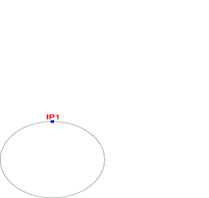
Refer to caption
Figure 12: Linear machine with a single interaction point (schematic)

We are interested in the invariant hh. We need the (usual) linear transform e:f2:superscript𝑒:absentsubscript𝑓2:e^{:f_{2}:} and the beam–beam interaction e:F:superscript𝑒:absent𝐹:e^{:F:}, i.e.

e:f2:e:F:=e:h:superscript𝑒:absentsubscript𝑓2:superscript𝑒:absent𝐹:superscript𝑒:absent:\displaystyle e^{:f_{2}:}\cdot e^{:F:}=e^{:{{h}}:} (387)

with (see before)

f2=μ2(x2β+βpx2)subscript𝑓2𝜇2superscript𝑥2𝛽𝛽subscriptsuperscript𝑝2𝑥\displaystyle f_{2}=-\frac{\mu}{2}\left(\frac{x^{2}}{\beta}+\beta p^{2}_{x}\right) (388)

and (see before)

F=0xdxf(x).𝐹superscriptsubscript0𝑥differential-dsuperscript𝑥𝑓superscript𝑥\displaystyle F=\displaystyle{\int_{0}^{x}}\,{\mathrm{d}}x^{\prime}f(x^{\prime}). (389)

For a Gaussian beam, we have for f(x)𝑓𝑥f(x) (see article on beam–beam effects [30])

f(x)=2x(1ex2/2σ2).𝑓𝑥2𝑥1superscript𝑒superscript𝑥22superscript𝜎2\displaystyle f(x)=\frac{2}{x}(1-e^{{-x^{2}}/{2\sigma^{2}}}). (390)

As usual, we go to action-angle variables ΨΨ\Psi, J𝐽J:

x=2JβsinΨ,p=2JβcosΨformulae-sequence𝑥2𝐽𝛽Ψ𝑝2𝐽𝛽Ψ\displaystyle x=\sqrt{2J\beta}\sin\Psi,\quad p=\sqrt{\frac{2J}{\beta}}\cos\Psi (391)

and write F(x)𝐹𝑥F(x) as a Fourier series:

F(x)=n=cn(J)einΨ.𝐹𝑥superscriptsubscript𝑛subscript𝑐𝑛𝐽superscriptei𝑛Ψ\displaystyle F(x)=\sum_{n=-\infty}^{\infty}c_{n}(J){\rm e}^{{\rm i}n\Psi}. (392)

With this transformation to action-angle variables, the generator f2subscript𝑓2f_{2} becomes very simple:

f2=μJsubscript𝑓2𝜇𝐽\displaystyle f_{2}=-\mu J (393)

and useful properties of Lie operators (e.g. [7, 6, 9])

:f2:g(J)=0,:f2:einΨ=inμeinΨ,g(:f2:)einΨ=g(inμ)einΨ\displaystyle:f_{2}:g(J)=0,\quad:f_{2}:{\rm e}^{{\rm i}n\Psi}={\rm i}n\mu{\rm e}^{{\rm i}n\Psi},\quad g(:f_{2}:){\rm e}^{{\rm i}n\Psi}=g({\rm i}n\mu){\rm e}^{{\rm i}n\Psi} (394)

and the formula (e.g. [7, 6, 9])

e:f2:e:F:=e:h:=exp[:f2+(:f2:1e:f2:)F+𝒪(F2):]\displaystyle e^{:f_{2}:}e^{:F:}=e^{:h:}=\exp\left[:f_{2}+\left(\frac{:f_{2}:}{1-e^{-:f_{2}:}}\right)F+{\cal{O}}(F^{2}):\right] (395)

give immediately for hh

h=μJ+ncn(J)inμ1einμeinΨ,𝜇𝐽subscript𝑛subscript𝑐𝑛𝐽i𝑛𝜇1superscriptei𝑛𝜇superscriptei𝑛Ψ\displaystyle h=-\mu J+\sum_{n}c_{n}(J)\frac{{\rm i}n\mu}{1-{\rm e}^{-{\rm}{\rm i}n\mu}}{\rm e}^{{\rm i}n\Psi}, (396)
h=μJ+ncn(J)nμ2sin(nμ/2)e(inΨ+inμ2).𝜇𝐽subscript𝑛subscript𝑐𝑛𝐽𝑛𝜇2𝑛𝜇2superscriptei𝑛Ψi𝑛𝜇2\displaystyle h=-\mu J+\sum_{n}c_{n}(J)\frac{n\mu}{2\sin({n\mu}/{2})}{\rm e}^{\left({\rm i}n\Psi+{\rm i}\frac{n\mu}{2}\right)}. (397)

Away from resonances, the normal-form transformation gives

hn=μJ+c0(J)=const.subscript𝑛𝜇𝐽subscript𝑐0𝐽const\displaystyle h_{n}=-\mu J+c_{0}(J)=\mathrm{const}. (398)

The expression

dc0(J)dJdsubscript𝑐0𝐽d𝐽\displaystyle\frac{{\rm d}c_{0}(J)}{{\rm d}J} (399)

gives the detuning with amplitude due to the beam–beam interaction.

The analysis for a single interaction point gives [27]

h=μJ+ncn(J)nμ2sin(nμ/2)e(inΨ+inμ2).𝜇𝐽subscript𝑛subscript𝑐𝑛𝐽𝑛𝜇2𝑛𝜇2superscriptei𝑛Ψi𝑛𝜇2\displaystyle h=-\mu J+\sum_{n}c_{n}(J)\frac{n\mu}{{{2\sin({n\mu}/{2})}}}{\rm e}^{\left({\rm i}n\Psi+{\rm i}\frac{n\mu}{2}\right)}. (400)

On resonance, we immediately find the conditions

Q=pn=μ2π𝑄𝑝𝑛𝜇2𝜋\displaystyle Q=\frac{p}{n}=\frac{\mu}{2\pi} (401)

with cn0subscript𝑐𝑛0c_{n}\neq 0:

sin(nπpn)=sin(pπ)0for all integerpformulae-sequence𝑛𝜋𝑝𝑛𝑝𝜋0for all integer𝑝\displaystyle\sin\left(\frac{n\pi p}{n}\right)=\sin(p\pi)\equiv 0\quad\mbox{for all integer}\leavevmode\nobreak\ p (402)

and hh diverges, finding automatically all resonance conditions.
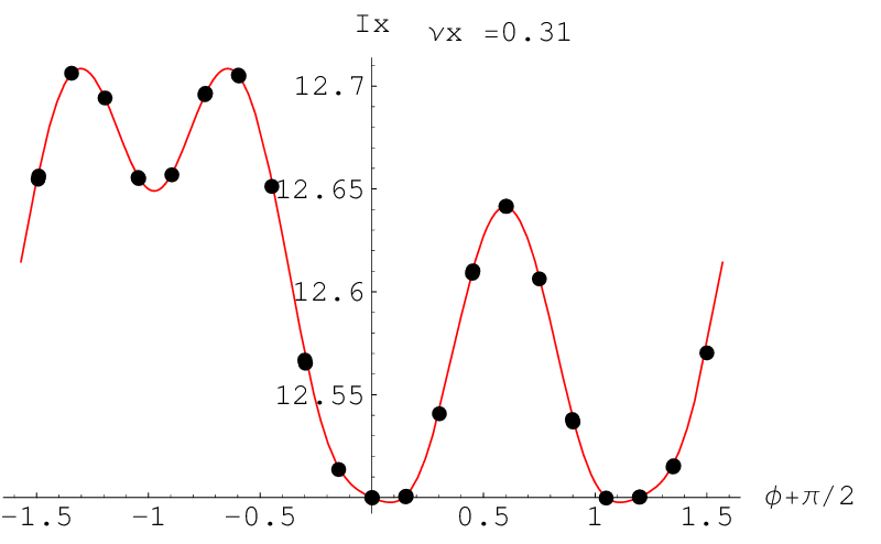
Refer to caption
Refer to caption
Figure 13: Turn by turn points in phase space from simulation program, comparison with invariant (full line).

To compare with particle tracking, a simple tracking code was used [27] and the turn by turn points in phase space are shown in \Freffig:fig15 for amplitudes of 5σxsubscript𝜎𝑥\sigma_{x} and 10σxsubscript𝜎𝑥\sigma_{x}. The figure also shows the beam–beam invariant as computed from the effective Hamiltonian compared with the tracking result [27]. The agreement is remarkable.

This technique can be used to analyse and compare the strengths of non-linear effects as demonstrated in [28] and used to derive scaling laws for long range beam–beam effects in the LHC [29].

0.8 Differential algebra

0.8.1 Motivation

Analytical formulas are usually difficult to derive and often rely on simplifications and assumptions. Although they may be fast to evaluate, they can only be used as guidance to more precise calculations. It is generally accepted that elaborate tracking codes provide the most reliable description of a non-linear system. Ideally, one should like to derive global quantities such as closed orbit, tunes or detuning from the tracking codes. The tracking of a complicated system relates the output numerically to the input producing a numerical map and one might ask whether it is possible to relate this output to global quantities in an easy way. More precisely, can a code be used to provide input to a description or formula such that these relate more directly to global quantities? This would free us from approximate analytical calculations. They would provide ‘analytical’ formulas although they are not analytical in the classical sense, which should be considered as symbolic [6]. A typical example of such an analytical derivation would be a Taylor series derived from a tracking code.

0.8.2 Taylor series as analytical formulas

Why are Taylor series useful in the analysis of beam dynamics, in particular stability for non-linear systems? Let us study the paraxial behaviour sketched in \Freffig:fig16. The red line indicates the ideal orbit while the blue lines are small deviations from this ideal orbit caused by distortions. If we understand how small deviations behave, we understand the system much better. Now remember the definition of the Taylor series:

f(a+Δx)=f(a)+n=1f(n)(a)n!Δxn,𝑓𝑎Δ𝑥𝑓𝑎superscriptsubscript𝑛1superscript𝑓𝑛𝑎𝑛Δsuperscript𝑥𝑛\displaystyle f(a+\Delta x)=f(a)+\sum_{n=1}^{\infty}\frac{f^{(n)}(a)}{n!}\Delta x^{n}, (403)
f(a+Δx)=f(a)+f(a)1!Δx1+f′′(a)2!Δx2+f′′′(a)3!Δx3+.𝑓𝑎Δ𝑥𝑓𝑎superscript𝑓𝑎1Δsuperscript𝑥1superscript𝑓′′𝑎2Δsuperscript𝑥2superscript𝑓′′′𝑎3Δsuperscript𝑥3\displaystyle f(a+\Delta x)=f(a)+\frac{{f^{\prime}(a)}}{{{1!}}}\Delta x^{1}+\frac{{f^{\prime\prime}(a)}}{{{2!}}}\Delta x^{2}+\frac{{f^{\prime\prime\prime}(a)}}{{{3!}}}\Delta x^{3}+\cdots. (404)

The coefficients determine the behaviour of small deviations ΔxΔ𝑥\Delta x from the ideal orbit x𝑥x, i.e. the Taylor expansion does a paraxial analysis of the system. If the function f(x)𝑓𝑥f(x) is represented by a Taylor series:

f(a+Δx)=f(a)+n=1f(n)(a)n!Δxn𝑓𝑎Δ𝑥𝑓𝑎superscriptsubscript𝑛1superscript𝑓𝑛𝑎𝑛Δsuperscript𝑥𝑛\displaystyle f(a+\Delta x)=f(a)+\sum_{n=1}^{\infty}\frac{f^{(n)}(a)}{n!}\Delta x^{n} (405)

and if it is truncated to the m𝑚mth order:

f(a+Δx)=f(a)+n=1mf(n)(a)n!Δxn.𝑓𝑎Δ𝑥𝑓𝑎superscriptsubscript𝑛1𝑚superscript𝑓𝑛𝑎𝑛Δsuperscript𝑥𝑛\displaystyle f(a+\Delta x)=f(a)+\sum_{n=1}^{m}\frac{f^{(n)}(a)}{n!}\Delta x^{n}. (406)

What is the relevance?

  • i)

    There is an equivalence between the function f(x)𝑓𝑥f(x) and the vector (f(a),f(a),f′′(a),,f(m)(a))𝑓𝑎superscript𝑓𝑎superscript𝑓′′𝑎superscript𝑓𝑚𝑎(f(a),f^{\prime}(a),f^{\prime\prime}(a),\ldots,f^{(m)}(a)).

  • ii)

    This vector is a truncated power series algebra (TPSA) representation of f(x)𝑓𝑥f(x) around a𝑎a.

It can be shown that the global quantities of interest are obtained more easily and conveniently from the Taylor series map [26]. Since it is derived from a symplectic tracking code, the corresponding map is also symplectic. Our problem is how to get these coefficients without extra work.
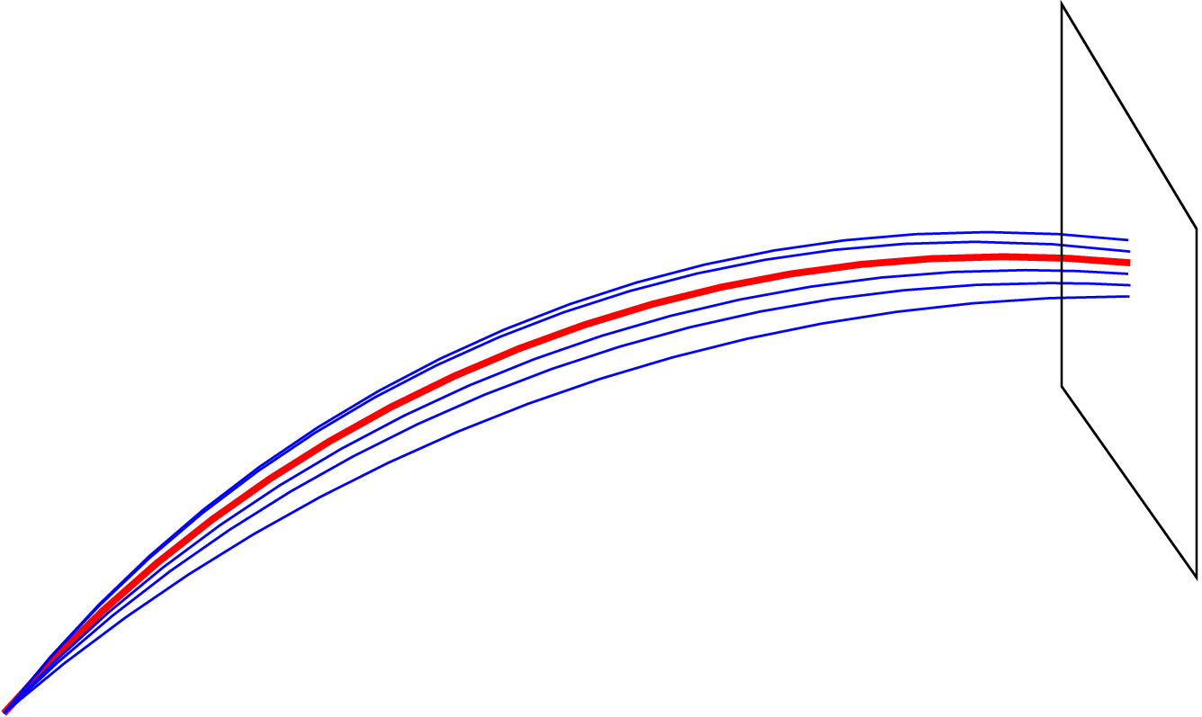
Refer to caption
Figure 14: Trajectories with small deviations from an ideal trajectory

The problem is getting the derivatives f(n)(a)superscript𝑓𝑛𝑎f^{(n)}(a) of f(x)𝑓𝑥f(x) at a𝑎a:

f(a)=f(a+ϵ)f(a)ϵ.superscript𝑓𝑎𝑓𝑎italic-ϵ𝑓𝑎italic-ϵ\displaystyle f^{\prime}(a)=\frac{f(a+\epsilon)-f(a)}{\epsilon}. (407)

The problems with this approach are as follows.

  • i)

    Need to subtract almost equal numbers and divide by small number.

  • ii)

    For higher orders f′′,f′′′,superscript𝑓′′superscript𝑓′′′f^{\prime\prime},f^{\prime\prime\prime},\ldots, it is hopeless to obtain the required accuracy.

  • iii)

    We can use differential algebra (DA) [24, 25, 26].

0.8.3 Basic concepts

The basic idea of differential algebra is the automatic differentiation of results produced by a tracking code to provide the coefficients of a Taylor series. Here we give the basic concepts of the mathematics [24, 25, 26]:

  1. 1.

    Define a pair (q0,q1subscript𝑞0subscript𝑞1q_{0},q_{1}),  with q0,q1subscript𝑞0subscript𝑞1q_{0},q_{1} real numbers.

  2. 2.

    Define operations on a pair like

    (q0,q1)+(r0,r1)=(q0+r0,q1+r1),subscript𝑞0subscript𝑞1subscript𝑟0subscript𝑟1subscript𝑞0subscript𝑟0subscript𝑞1subscript𝑟1\displaystyle(q_{0},q_{1})+(r_{0},r_{1})=(q_{0}+r_{0},q_{1}+r_{1}), (408)
    c(q0,q1)=(cq0,cq1),𝑐subscript𝑞0subscript𝑞1𝑐subscript𝑞0𝑐subscript𝑞1\displaystyle c\cdot(q_{0},q_{1})=(c\cdot q_{0},c\cdot q_{1}), (409)
    (q0,q1)(r0,r1)=(q0r0,q0r1+q1r0).subscript𝑞0subscript𝑞1subscript𝑟0subscript𝑟1subscript𝑞0subscript𝑟0subscript𝑞0subscript𝑟1subscript𝑞1subscript𝑟0\displaystyle(q_{0},q_{1})\cdot(r_{0},r_{1})=(q_{0}\cdot r_{0},q_{0}\cdot r_{1}+q_{1}\cdot r_{0}). (410)
  3. 3.

    And some ordering:

    (q0,q1)<(r0,r1)ifq0<r0or(q0=r0andq1<r1),formulae-sequencesubscript𝑞0subscript𝑞1subscript𝑟0subscript𝑟1ifsubscript𝑞0subscript𝑟0orsubscript𝑞0subscript𝑟0andsubscript𝑞1subscript𝑟1\displaystyle(q_{0},q_{1})<(r_{0},r_{1})\quad{\mathrm{if}}\ q_{0}<r_{0}\ {\mathrm{or}}\ (q_{0}=r_{0}\ {\mathrm{and}}\ q_{1}<r_{1}), (411)
    (q0,q1)>(r0,r1)ifq0>r0or(q0=r0andq1>r1).formulae-sequencesubscript𝑞0subscript𝑞1subscript𝑟0subscript𝑟1ifsubscript𝑞0subscript𝑟0orsubscript𝑞0subscript𝑟0andsubscript𝑞1subscript𝑟1\displaystyle(q_{0},q_{1})>(r_{0},r_{1})\quad{\mathrm{if}}\ q_{0}>r_{0}\ {\mathrm{or}}\ (q_{0}=r_{0}\ {\mathrm{and}}\ q_{1}>r_{1}). (412)
  4. 4.

    This implies something strange:

    (0,0)<(0,1)<(r,0)(foranypositiver),0001𝑟0foranypositive𝑟\displaystyle(0,0)<(0,1)<(r,0)\ ({\mathrm{for\leavevmode\nobreak\ any\leavevmode\nobreak\ positive}}\leavevmode\nobreak\ r), (413)
    (0,1)(0,1)=(0,0)(0,1)=(0,0).0101000100\displaystyle(0,1)\cdot(0,1)=(0,0)\rightarrow(0,1)=\sqrt{(0,0)}. (414)

    This means that (0, 1) is between 0 and any real number \rightarrow infinitely small. Therefore we call this a ‘differential unit’ d=(0,1)=δ𝑑01𝛿d=(0,1)=\delta.

Of course (q,0)𝑞0(q,0) is just the real number q𝑞q and we define the ‘real part’ and ‘differential part’ (a bit like complex numbers):

q0=(q0,q1)andq1=𝒟(q0,q1).formulae-sequencesubscript𝑞0subscript𝑞0subscript𝑞1andsubscript𝑞1𝒟subscript𝑞0subscript𝑞1\displaystyle q_{0}={\cal{R}}(q_{0},q_{1})\quad{\mathrm{and}}\quad q_{1}={\cal{D}}(q_{0},q_{1}). (415)

With our rules, we can further see that

(1,0)(q0,q1)=(q0,q1),10subscript𝑞0subscript𝑞1subscript𝑞0subscript𝑞1\displaystyle(1,0)\cdot(q_{0},q_{1})=(q_{0},q_{1}), (416)
(q0,q1)1=(1q0,q1q02).superscriptsubscript𝑞0subscript𝑞111subscript𝑞0subscript𝑞1superscriptsubscript𝑞02\displaystyle(q_{0},q_{1})\leavevmode\nobreak\ ^{-1}=\left(\frac{1}{q_{0}},-\frac{q_{1}}{q_{0}^{2}}\right). (417)

Now we let a function f𝑓f act on the pair (or vector) using our rules. For example,

f(x)f(x,0)𝑓𝑥𝑓𝑥0\displaystyle f(x)\rightarrow f(x,0) (418)

acts like the function f𝑓f on the real variable x𝑥x:

f(x)=[f(x,0)].𝑓𝑥delimited-[]𝑓𝑥0\displaystyle f(x)={\cal{R}}[f(x,0)]. (419)

What about the differential part 𝒟𝒟\cal{D}?

For a function f(x)𝑓𝑥f(x), without proof,

𝒟[f(x+d)]=𝒟[f((x,0)+(0,1))]=𝒟[f(x,1)]=f(x).𝒟delimited-[]𝑓𝑥𝑑𝒟delimited-[]𝑓𝑥001𝒟delimited-[]𝑓𝑥1superscript𝑓𝑥\displaystyle{\cal{D}}[f(x+d)]={\cal{D}}[f((x,0)+(0,1))]={\cal{D}}[f(x,1)]=f^{\prime}(x). (420)

The differential part of the output is the first-order derivative of the function f(x)𝑓𝑥f(x). To demonstrate this, it is done most easily by looking at an example.

Assume for the function f(x)𝑓𝑥f(x):

f(x)=x2+1x;𝑓𝑥superscript𝑥21𝑥\displaystyle f(x)=x^{2}+\frac{1}{x}; (421)

then, using school calculus, we can get the derivative:

f(x)=2x1x2.superscript𝑓𝑥2𝑥1superscript𝑥2\displaystyle f^{\prime}(x)=2x-\frac{1}{x^{2}}. (422)

For x=2𝑥2x=2, we obtain

f(2)=92,f(2)=154.formulae-sequence𝑓292superscript𝑓2154\displaystyle f(2)=\frac{9}{2},f^{\prime}(2)=\frac{15}{4}. (423)

Now we proceed with the same function and use the operations defined by the differential algebra. For x𝑥x in

f(x)=x2+1x,𝑓𝑥superscript𝑥21𝑥\displaystyle f(x)=x^{2}+\frac{1}{x}, (424)

we substitute x(x,1)=(2,1)𝑥𝑥121x\rightarrow(x,1)=(2,1) and use our rules:

f[(2,1)]𝑓delimited-[]21\displaystyle f[(2,1)] =\displaystyle= (2,1)2+(2,1)1superscript212superscript211\displaystyle(2,1)^{2}+(2,1)^{-1} (425)
=\displaystyle= (4,4)+(12,14)441214\displaystyle(4,4)+\left(\frac{1}{2},-\frac{1}{4}\right) (426)
=\displaystyle= (92,154)=(f(2),f(2)).92154𝑓2superscript𝑓2\displaystyle\left(\frac{9}{2},\frac{15}{4}\right)=(f(2),f^{\prime}(2)). (427)

The computation of derivatives becomes an algebraic problem, no need for small numbers, it is exact.

0.8.4 Differential algebra: higher orders and more variables

Higher orders

The algorithm can be extended to higher order, let us say of order N𝑁N:

  1. 1.

    the pair (q0,1subscript𝑞01q_{0},1) becomes a vector of order N𝑁N, (q0,1)(q0,1,0,0,,0)subscript𝑞01subscript𝑞01000(q_{0},1)\rightarrow(q_{0},1,0,0,\ldots,0), δ=(0,1,0,0,0,)𝛿01000\delta=(0,1,0,0,0,\ldots);

  2. 2.

    (q0,q1,q2,,qN)+(r0,r1,r2,,rN)=(s0,s1,s2,,sN),subscript𝑞0subscript𝑞1subscript𝑞2subscript𝑞𝑁subscript𝑟0subscript𝑟1subscript𝑟2subscript𝑟𝑁subscript𝑠0subscript𝑠1subscript𝑠2subscript𝑠𝑁(q_{0},q_{1},q_{2},\ldots,q_{N})+(r_{0},r_{1},r_{2},\ldots,r_{N})=(s_{0},s_{1},s_{2},\ldots,s_{N}), with si=qi+risubscript𝑠𝑖subscript𝑞𝑖subscript𝑟𝑖s_{i}=q_{i}+r_{i};

  3. 3.

    c(q0,q1,q2,,qN)=(cq0,cq1,cq2,,cqN)𝑐subscript𝑞0subscript𝑞1subscript𝑞2subscript𝑞𝑁𝑐subscript𝑞0𝑐subscript𝑞1𝑐subscript𝑞2𝑐subscript𝑞𝑁c\cdot(q_{0},q_{1},q_{2},\ldots,q_{N})=(c\cdot q_{0},c\cdot q_{1},c\cdot q_{2},\ldots,c\cdot q_{N});

  4. 4.

    (q0,q1,q2,,qN)(r0,r1,r2,,rN)=(s0,s1,s2,,sN);subscript𝑞0subscript𝑞1subscript𝑞2subscript𝑞𝑁subscript𝑟0subscript𝑟1subscript𝑟2subscript𝑟𝑁subscript𝑠0subscript𝑠1subscript𝑠2subscript𝑠𝑁(q_{0},q_{1},q_{2},\ldots,q_{N})\cdot(r_{0},r_{1},r_{2},\ldots,r_{N})=(s_{0},s_{1},s_{2},\ldots,s_{N}); with

    si=k=0ii!k!(ik)!qkrik.subscript𝑠𝑖superscriptsubscript𝑘0𝑖𝑖𝑘𝑖𝑘subscript𝑞𝑘subscript𝑟𝑖𝑘\displaystyle s_{i}=\sum_{k=0}^{i}\frac{i!}{k!(i-k)!}q_{k}r_{i-k}. (428)

Additional variables

We can go to more dimensions, i.e. more variables, with rather small modifications. If we had started with

x=(a,1,0,0,0,),𝑥𝑎1000\displaystyle x=(a,1,0,0,0,\ldots), (429)

we would get

f(x)=(f(a),f(a),f′′(a),f′′′(a),,f(n)(a)).𝑓𝑥𝑓𝑎superscript𝑓𝑎superscript𝑓′′𝑎superscript𝑓′′′𝑎superscript𝑓𝑛𝑎\displaystyle f(x)=(f(a),f^{\prime}(a),f^{\prime\prime}(a),f^{\prime\prime\prime}(a),\ldots,f^{(n)}(a)). (430)

This can be extended to more variables x𝑥xy𝑦y:

x=(a,1,0,0,0,),dx=(0,1,0,0,0,),formulae-sequence𝑥𝑎1000d𝑥01000\displaystyle x=(a,1,0,0,0,\ldots),\quad{\rm d}x=(0,1,0,0,0,\ldots), (431)
y=(b,0,1,0,0,),dy=(0,0,1,0,0,)formulae-sequence𝑦𝑏0100d𝑦00100\displaystyle y=(b,0,1,0,0,\ldots),\quad{\rm d}y=(0,0,1,0,0,\ldots) (432)

and we get (with more complicated multiplication rules [6, 22])

f((x+dx),y+dy))=(f,fx,fy,2fx2,2fxy,)(x,y).\displaystyle f((x+{\rm d}x),y+{\rm d}y))=\left(f,\frac{\partial f}{\partial x},\frac{\partial f}{\partial y},\frac{\partial^{2}f}{\partial x^{2}},\frac{\partial^{2}f}{\partial x\partial y},\ldots\right)(x,y). (433)

0.8.5 Examples

To demonstrate the algorithm and how it can be used in practice, I show a few examples.

Simple example

Below is a very simple program to compute sin(π/6)𝜋6\sin(\pi/6). In the first case (DATEST1) regular data types are used while in the second program (DATEST2) the usual data types are replaced by the type of a Taylor map (in the program called my_taylor).   
  
  
PROGRAM DATEST1 use my_own_da real(8) x,z,dx
my_order=3
dx=0.0 x=3.141592653/6.0 + dx call track(x, z) call print(z, 6) END PROGRAM DATEST1 SUBROUTINE TRACK(a, b) use my_own_da real(8) a,b
b = sin(a)
END SUBROUTINE TRACK
PROGRAM DATEST2 use my_own_da type(my_taylor) x,z,dx
my_order=3
dx=1.0.mono.1    !this is our (0,1)
x=3.141592653/6.0 + dx
call track(x, z) call print(z, 6) END PROGRAM DATEST2 SUBROUTINE TRACK(a, b) use my_own_da type(my_taylor) a,b
b = sin(a)
END SUBROUTINE TRACK
If we run the two programs, we obtain for the two outputs
   
   
(0,0) 0.5000000000000E+00 (0,0) 0.5000000000000E+00 (1,0) 0.8660254037844E+00 (0,1) 0.0000000000000E+00 (2,0) -0.2500000000000E+00 (0,2) 0.0000000000000E+00 (1,1) 0.0000000000000E+00 (3,0) -0.1443375672974E+00 (0,3) 0.0000000000000E+00 (2,1) 0.0000000000000E+00 (1,2) 0.0000000000000E+00 We have sin(π/6)=0.5𝜋60.5\sin({\pi}/{6})=0.5 all right, but what is the rest? Let us look at

sin(π6+Δx)=sin(π6)+cos(π6)Δx112sin(π6)Δx216cos(π6)Δx3,𝜋6Δ𝑥𝜋6𝜋6Δsuperscript𝑥112𝜋6Δsuperscript𝑥216𝜋6Δsuperscript𝑥3\displaystyle\sin\left(\frac{\pi}{6}+\Delta x\right)=\sin\left(\frac{\pi}{6}\right)+\cos\left(\frac{\pi}{6}\right)\Delta x^{1}-\frac{1}{2}\sin\left(\frac{\pi}{6}\right)\Delta x^{2}-\frac{1}{6}\cos\left(\frac{\pi}{6}\right)\Delta x^{3}, (434)

i.e. we have found the coefficients of the sine𝑠𝑖𝑛𝑒sine evaluated at sin(π/6)𝜋6\sin({\pi}/{6}).

  • i)

    We have used a simple algorithm here (sin\sin) but it can be anything and very complex.

  • ii)

    We can compute non-linear maps as a Taylor expansion of anything the program computes.

  • iii)

    Simply by:

    • a)

      replacing regular (e.g. real) types by TPSA types (my_taylor), i.e. variables x,p𝑥𝑝x,p are automatically replaced by (x,1,0,)𝑥10(x,1,0,\ldots) and (p,0,1,0,)𝑝010(p,0,1,0,\ldots) etc.;

    • b)

      operators and functions (+,,,=,,exp,sin,+,-,*,=,\ldots,\exp,\sin,\ldots) are automatically overloaded, i.e. behave according to the new type.

A FODO lattice

Another example.

  • \bullet

    Track through a simple FODO lattice described as:

  • QF - DRIFT - QD

  • Integrate 100 steps in the quadrupoles.

  • Now we use three variables:

  • x, p, Δp=(z(1),z(2),z(3))Δ𝑝𝑧1𝑧2𝑧3\Delta p=(z(1),z(2),z(3)) (third variable needed to compute the chromaticity).


PROGRAM FODO1

use my_own_da

use my_analysis

type(my_taylor) z(3)

type(normalform) NORMAL

type(my_map) M,id

real(dp) L,DL,k1,k3,fix(3)

integer i,nstep

my_order=4  ! maximum order 4

fix=0.0 ! fixed point

id=1

z=fix+id

LC=62.5     ! half cell length

L=3.0     ! quadrupole length

nstep=100

DL=L/nstep

k1=0.003     ! quadrupole strength

do i=1,nstep     ! track through quadrupole

z(1)=z(1)+DL/2*z(2)

z(2)=z(2)-k1*DL*z(1)/(1 + z(3))

z(1)=z(1)+DL/2*z(2)

enddo

z(1)=z(1)+LC*z(2)     ! drift of half cell length

do i=1,nstep     ! track through quadrupole

z(1)=z(1)+DL/2*z(2)

z(2)=z(2)-k1*DL*z(1)/(1 + z(3))

z(1)=z(1)+DL/2*z(2)

enddo

z(1)=z(1)+LC*z(2)     ! drift of half cell length

call print(z(1),6)

call print(z(2),6)

M=z

NORMAL=M

write(6,*) normal%tune, normal%dtune_da

end program fodo1


We get the result of the program:
   
   
(0,0,0) 0.9442511679729E-01 (0,0,1) -0.9729519276183E-01 (1,0,0) 0.6972061935061E-01 (0,1,0) 0.1677727932585E+03 (1,0,1) 0.1266775134236E+01 (0,1,1)-0.3643444875882E+02 (1,0,2)-0.1603248617779E+01 (0,1,2) 0.3609522079691E+02 (1,0,3) 0.1939697138318E+01 (0,1,3)-0.3575511053483E+02 (1,0,0)-0.5300319873866E-02 (0,1,0) 0.1588490329398E+01 (1,0,1) 0.1060055415702E-01 (0,1,1)-0.5832024543075E+00 (1,0,2)-0.1590066005419E-01 (0,1,2) 0.5779004431627E+00 (1,0,3) 0.2120059477024E-01 (0,1,3)-0.5725843143370E+00 With only linear elements in the Taylor expansion, the result for the matrix per cell is Δxf=0.06972Δxi+167.77Δpi,Δsubscript𝑥𝑓0.06972Δsubscript𝑥𝑖167.77Δsubscript𝑝𝑖\displaystyle\Delta x_{f}={{0.06972}}\Delta x_{i}+{{167.77}}\Delta p_{i}, (435) Δpf=0.00530Δxi+1.5885Δpi.Δsubscript𝑝𝑓0.00530Δsubscript𝑥𝑖1.5885Δsubscript𝑝𝑖\displaystyle\Delta p_{f}={{-0.00530}}\Delta x_{i}+{{1.5885}}\Delta p_{i}. (436) The outputs from the normal-form analysis are (per cell) Tune = 0.094425, Chromaticity = –0.097295.   
We add now to this example a thin octupole:


PROGRAM FODO3 use my_own_da use my_analysis type(my_taylor) z(3) type(normalform) NORMAL type(my_map) M,id real(dp) L,DL,k1,k3,fix(3) integer i,nstep my_order=4  ! maximum order 4 fix=0.0 ! fixed point id=1 z=fix+id LC=62.5     ! half cell length L=3.0     ! quadrupole length nstep=100 DL=L/nstep k1=0.003     ! quadrupole strength k3=0.01     ! octupole strength do i=1,nstep     ! track through quadrupole z(1)=z(1)+DL/2*z(2) z(2)=z(2)-k1*DL*z(1)/(1 + z(3)) z(1)=z(1)+DL/2*z(2) enddo z(2)=z(2)-k3*z(1)**3/(1 + z(3))  ! octupole kick z(1)=z(1)+LC*z(2)     ! drift of half cell length do i=1,nstep     ! track through quadrupole z(1)=z(1)+DL/2*z(2) z(2)=z(2)-k1*DL*z(1)/(1 + z(3)) z(1)=z(1)+DL/2*z(2) enddo z(1)=z(1)+LC*z(2)     ! drift of half cell length call print(z(1),6) call print(z(2),6) M=z NORMAL=M write(6,*) normal%tune, normal%dtune_da end program fodo3    
The result of this program is now

(0,0,0) 0.9442511679729E-01

(0,0,1) -0.9729519276183E-01

(2,0,0) 0.5374370086899E+02

(0,2,0) 0.5374370086899E+02

(0,0,2) 0.1018391758451E+00

(2,0,1) 0.2035776281196E+02

……….

(1,0,0) 0.6972061935061E-01

(0,1,0) 0.1677727932585E+03

(1,0,1) 0.1266775134236E+01

(0,1,1)-0.3643444875882E+02

(3,0,0)-0.1586519461687E+01

(2,1,0)-0.1440953324752E+02

(1,2,0)-0.4362477179879E+02

……….

(1,0,0)-0.5300319873866E-02

(0,1,0) 0.1588490329398E+01

(1,0,1) 0.1060055415702E-01

(0,1,1)-0.5832024543075E+00

(3,0,0)-0.1519218878892E-01

Now there are non-linear elements in the Taylor expansion; the outputs from the normal-form analysis are (per cell)
Tune = 0.094425,
Chromaticity = -0.097295.
The detuning with amplitude is 53.74. This is the result we had for the analytical calculation for an octupole in the previous section.

Analysis using the normal form

Remember the normal-form transformation

𝒜𝒜1=.𝒜superscript𝒜1\displaystyle{\cal{A}}{\cal{M}}{\cal{A}}^{-1}={\cal{R}}. (437)

The type normalform in the demonstration package also contains the maps 𝒜𝒜{\cal{A}} and {\cal{R}}:

j2=(x**2+p**2)*NORMAL%A**(-1)

Remember that x**2+p**2 is the tilted ellipse and 𝒜1superscript𝒜1{\cal{A}}^{-1} the transformation to the normal form, containing the optical parameters α𝛼\alpha, β𝛽\beta, γ𝛾\gamma.

We can obtain the optical functions because:

  • i)

    β𝛽\beta is the coefficient of p**2 of invariant j2;

  • ii)

    α𝛼\alpha is the coefficient of x*p of invariant j2;

  • iii)

    γ𝛾\gamma is the coefficient of x**2 of invariant j2.

To obtain the linear optical parameters in our code, use something like

β𝛽\beta = j2.sub.beta,

α𝛼\alpha = 0.5*j2.sub.twoalpha,

γ𝛾\gamma = j2.sub.gamma;

we obtain (here at the end of the cell) β=300.080714𝛽300.080714\beta=300.080714, α=1.358246𝛼1.358246\alpha=-1.358246, γ= 9.480224𝛾9.480224\gamma=\leavevmode\nobreak\ 9.480224E-3.

0.9 Summary and epilogue

In this article I have tried to show the need for a new paradigm and a new framework for the study and analysis of non-linear beam dynamics is accelerators. Emphasis was put on the use of new numerical and computational techniques which allow better (and simpler) treatment. Putting aside pedagogical issues, the dreadful use of approximations and the limitations in the standard treatments can be avoided in the era of powerful computers and computing techniques. For example, the evaluation of resonances can be easily carried beyond leading orders and brings us well ahead of standard models. Therefore, I advocate the use of contemporary tools which unify linear, non-linear, coupled, decoupled and symplectic treatments. They can be treated and handled at the same time and the theoretical framework is simplified in the humble opinion of the author. The ideas presented in this article are based on the work of numerous people and at this point I hope that the next generation of accelerator physicists will continue (or start) to follow in this direction.

Acknowledgements

I wish to thank my colleagues for their interest and many discussions on this topic. I am glad to thank the members of the SSC Central Design Group whose contributions to the topics presented here have inspired me to enter this subject. I am particularly grateful to Prof. Alex Dragt who was the first to apply the technique of Lie transformation to non-linear problems in accelerator physics. For their contributions and many discussions I appreciate the collaboration with Dr Dobrin Kaltchev and Dr Etienne Forest, the latter for the TPSA demonstration program used during the preparation of this article.

References

  • [1] E. Courant and H. Snyder, Ann. Phys. 3 (1958) 1.
  • [2] H. Wiedemann, Particle Accelerator Physics – Basic Principles and Linear Beam Dynamics (Springer, Berlin, 1993).
  • [3] A. Chao and M. Tigner, Handbook of Accelerator Physics and Engineering (World Scientific, Singapore, 1998).
  • [4] H. Poincaré, Les Methods Nouvelles de la Mecanique Celeste (Gauthier-Villars, Paris, 1892).
  • [5] A.J. Lichtenberg and M.A. Lieberman, Regular and Chaotic Dynamics (Applied Mathematical Sciences No. 38, Springer, New York, 1983).
  • [6] E. Forest, Beam Dynamics – A New Attitude and Framework (Harwood Academic, Amsterdam, 1998).
  • [7] A. Chao, Lecture notes on topics in accelerator physics, SLAC (2001).
  • [8] A. Dragt, Lie Methods for Non-linear Dynamics with Applications to Accelerator Physics, (University of Maryland, 2009).
  • [9] W. Herr and E. Forest, Non-linear Dynamics in Accelerators, Landolt-Börnstein, New Series Vol. I/21C, Accelerators and Colliders, Ed. S. Myers and H. Schopper (Springer, Berlin, 2013), p.3-23].
  • [10] B. Holzer, Transverse Dynamics, these proceedings (CAS 2013).
  • [11] A. Dragt, AIP Proc. 87 (1981) 147.
  • [12] A. Dragt et al., Annu. Rev. Nucl. Part. Sci. 38 (1988) 455.
  • [13] A. Dragt et al., Phys. Rev. A45 (1992) 2572.
  • [14] F. Hausdorff, Ber. Verh. Saechs. Akad. Wiss. (Leipz.) 58 (1906) 19.
  • [15] J. Campbell, Proc. Lond. Math. Soc. 28 (1897) 381; ibid 29 (1898) 14.
  • [16] H. Poincar , C. R. Acad. Sci. Paris 128 (1899) 1065; Camb. Philos. Trans. 18 (1899) 220.
  • [17] H. Baker, Proc. Lond. Math. Soc. (1) 34 (1902) 347; ibid (1) 35 (1903) 333; ibid (2) 3 (1905) 24.
  • [18] E. Forest and R. Ruth, Physica D43 (1990) 105.
  • [19] H. Yoshida, Phys. Lett. A150 (1990) 262.
  • [20] H. Goldstein, Classical Mechanics (Addison Wesley, London, 1959).
  • [21] A. Wolski, Lecture notes on non-linear single particle dynamics, University of Liverpool (2006).
  • [22] E. Forest, M. Berz and J. Irwin, SSC Report SSC-166 (1992).
  • [23] E. Forest, D. Douglas and B. Leemann, Nucl. Instrum. Methods A258 (1987) 355.
  • [24] M. Berz, H.C. Hofmann and H. Wollnick, Nucl. Instrum. Methods A258 (1987) 402.
  • [25] M. Berz, Part. Accel. 24 (1989) 109.
  • [26] M. Berz, Modern Map Methods in Particle Beam Physics (Academic Press, San Diego, 1999).
  • [27] W. Herr and D. Kaltchev, Effect of phase advance between interaction points in the LHC on the beam–beam interaction, LHC Project Report 1082 (2008), unpublished.
  • [28] D. Kaltchev, Analysis of long range studies in the LHC – comparison with the model, ICFA Beam–beam Workshop, CERN (2013).
  • [29] R. Assmann et al., Results from long range studies in the LHC – scaling with beam separation and intensity, CERN-ATS-Note-2012-070 MD (2012).
  • [30] T. Pieloni, Beam–beam Effects, these proceedings (CAS 2013).