The first two authors contributed equally to this paper.
Link community detection through global optimization and the inverse resolution limit of partition density
Abstract
We investigate the possibility of global optimization-based overlapping community detection, using link community framework. We first show that partition density, the original quality function used in link community detection method, is not suitable as a quality function for global optimization because it prefers breaking communities into triangles except in highly limited conditions. We analytically derive those conditions and confirm it with computational results on direct optimization of various synthetic and real-world networks. To overcome this limitation, we propose alternative approaches combining the weighted line graph transformation and existing quality functions for node-based communities. We suggest a new line graph weighting scheme, a normalized Jaccard index. Computational results show that community detection using the weighted line graphs generated with the normalized Jaccard index leads to a more accurate community structure.
pacs:
89.75.-k,89.75.HcI Introduction
Finding community structure is essential in understanding meso-scale organization of complex networks. Most commonly, community detection is performed by assigning nodes into groups that optimizes a quality function, which measures how meaningful the grouping is Fortunato (2010). Community detection methods can be classified into two main categories based on whether they allow a node to be included in multiple communities (overlapping communities) or not (disjoint communities). For the latter, the most widely used quality measure is modularity Newman and Girvan (2004). It measures, for each community, the difference between the number of links between the nodes in the same community and the expected number of links when the network is randomly re-wired. Various optimization methods have been applied to optimize modularity Fortunato (2010); Lee et al. (2012); Zhang et al. (2009); Bagrow (2012). Although modularity has been widely applied to analyze various social and biological networks Lee and Lee (2013); Lee et al. (2013), several drawbacks have been found Fortunato (2010); Good et al. (2010). One of the most important problem is so-called “resolution limit” Fortunato and Barthelemy (2007). As a network becomes larger, the expected number of links within a group decrease, eventually leading to the situation where even merging two distinct complete cliques is better than keeping them separated. Thus, small but meaningful communities in a large network may not be detectable with modularity.
Meanwhile, it has been argued that communities overlap pervasively in many real-world networks Palla et al. (2005); Ahn et al. (2010). For example, in social networks, each person participates in multiple social groups. In biological networks, a protein may play diverse roles in multiple biological processes Lee et al. (2011a); Lee and Lee (2013); Lee et al. (2013); Malik et al. (2014). Among many overlapping community detection methods that have been suggested Palla et al. (2005); Lancichinetti et al. (2009); Ahn et al. (2010); Evans and Lambiotte (2010); Viamontes Esquivel and Rosvall (2011); Lancichinetti et al. (2011); Yang and Leskovec (2012); Xie et al. (2013); Gopalan and Blei (2013); Zhang et al. (2013), here we focus on the “link community” paradigm, where the communities are redefined as sets of links (edges) rather than nodes Ahn et al. (2010); Evans and Lambiotte (2010). This framework provides a clean way to handle pervasive overlaps between communities because identifying communities of links in the original graph is equivalent to identifying disjoint communities of nodes in the “line graph” of the original graph West et al. (2001); Evans and Lambiotte (2009, 2010); Ahn et al. (2010).
As modularity is not well-defined for the link-groupings, “partition density” was proposed as a quality function for link communities Ahn et al. (2010). For an undirected and unweighted network, imagine a disjoint partition of links where is the number of link communities. The local partition density of a link community is:
| (1) |
where is the number of links in the community , and are the minimum and maximum possible numbers of links between the induced nodes that the links in touch, assuming that the nodes in are connected, and is the number of the induced nodes. If the induced nodes are not connected, is set to . The partition density of the network is:
| (2) |
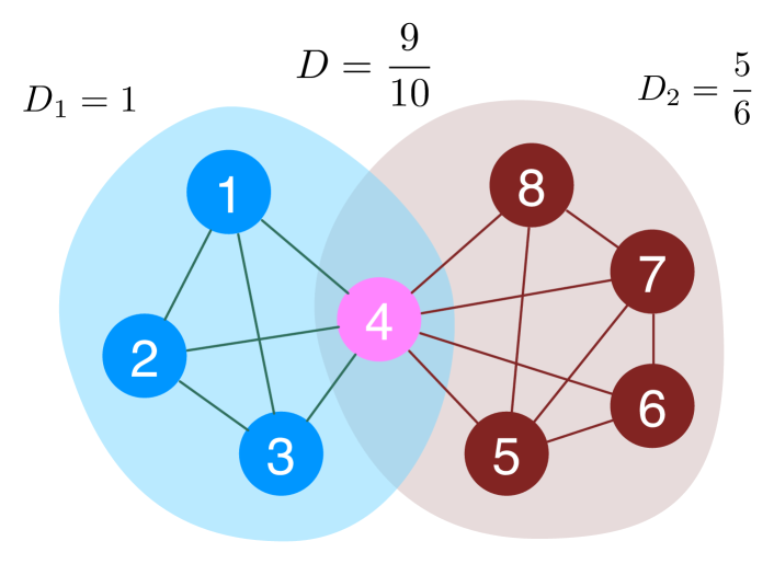
where is the number of links in the network. Figure 1 shows a toy example that illustrates how partition density is calculated. By employing hierarchical clustering and Jaccard index-based link similarity measure, a previous study argued that partition density can be used to identify meaningful communities evaluated by the similarity of the metadata of the nodes Ahn et al. (2010). Additionally, as partition density only uses local information, it was suggested that partition density is free from the problem of resolution limit observed in modularity Fortunato and Barthelemy (2007); Ahn et al. (2010).
Here we show, while partition density may not have the problem of the resolution limit, that partition density suffers from an inverse resolution limit: a strong preference towards small cliques, due to the fact that partition density is a simple density measure that does not take any null model into account. We show that direct optimization of partition density simply identifies most 3-cliques (triangle) in the network. We analyze when exactly triangles are favored or not by using toy models and a systematic classification of triangles based on their connectivity. Our analysis demonstrates that larger communities are only favored in highly limited conditions. We then explore alternative direct-optimization approaches—a combination of weighted line graph transformation and other quality functions—to identify overlapping communities through the link community framework.
II Preference to triangles
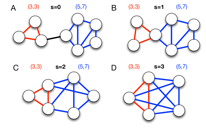
As partition density has been successfully applied previously, it is natural to ask whether it can be used as a quality function subject to direct global optimization, as in the case of modularity. However, as we will show below, partition density heavily suffers from its preference towards small cliques since it measures pure density without incorporating any statistical null model. In this section, we examine partition density’s strong preference towards small cliques in detail. Without loss of generality, we can imagine that there is one triangle in a local link community . Let us assume that shares nodes with the rest of the link community containing nodes and edges. There are four possible choices for the value of which is shown in Figure 2.
By definition, a partition density of the community is:
| (3) |
where is the total number of links in the whole network, and are the number of nodes and links in the community , respectively.
The partition density and of the triangle and the subnetwork are
| (4) |
and
| (5) |
respectively.
The condition where the separation of triangle is preferred can be determined by solving the following inequality:
| (6) | ||||
| (7) |
If is negative, the triangle and its neighboring link community will merge into one link community, otherwise they prefer to be separated.
When ,
| (8) |
If is replaced with the minimum number of links between nodes, , , which is positive. Because is an increasing function of , is always positive; the formation of triangle is always preferred.
Similarly, if ,
| (9) |
Because , the denominator is positive, and the coefficient of , , is also positive. Fixing , is a monotonically increasing function of if is larger than , which is smaller than the minimum of , . Replacing by , is positive. Hence is always positive for .
If ,
| (10) |
Similar analysis shows that fixing , is a monotonically increasing function of if is larger than , which is larger than the minimum of , . Replacing by , is positive except for the case . For , is negative when has its minimum value . keeps decreasing as increases until . After , increases and becomes positive again when . Hence is always positive except in the case and .
This result clearly shows why triangles are preferred by the current definition of partition density. It indicates that, for a given link community consisting of more than 4 nodes, if there exists an independent triangle that contains a node that is not connected with the rest of nodes in the same community, the triangle is always separated.
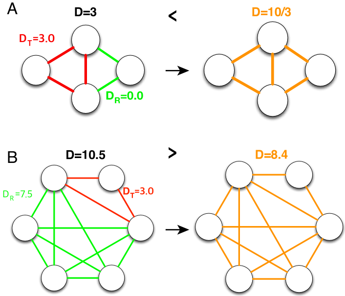
Figure 3 shows the examples of cases. In Figure 3A, the partition density of the green triangle is , and the rest of links form a linear community with the partition density of , which results in the total partition density of 3. Here, the denominator in eq. 2 is omitted since it is a constant. However, when the two link communities are merged, the partition density becomes 10/3, which makes the separation of triangle unfavorable. In Figure 3B, a link community has more than five edges and an independent triangle. In the right side of Figure 3B, a link community consists of 6 nodes and 12 edges and contains an independent triangle. The partition density of the community is 8.4. However, if the independent triangle is separated, the sum of partition densities becomes 10.5, which makes the separation of triangle favorable.
If , which means that there is no independent triangle in the community, can be written as below:
| (11) |
is negative if the following condition is satisfied:
| (12) |
Thus, a merged link community with nodes and links is non-separable if the following condition is satisfied
| (13) |
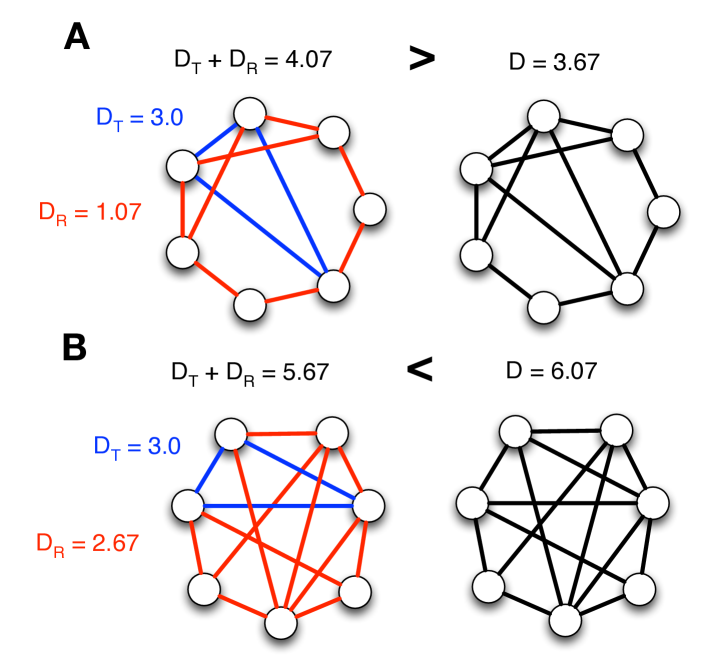
In other words, if eq. 13 is not satisfied, a link community is separable although there is no independent triangle in it. Two examples of the case of are shown in Figure 4. The first example does not satisfy eq. 13 (Figure 4A). Thus it prefers to be separated although there is no independent triangle. The partition density of the merged link community is 3.67, while the sum of partition densities of two separated link communities is 4.07. On the other hand, the second example corresponds to the case where eq. 13 is satisfied (Figure 4B). The sum of partition densities of separated link communities, 5.67, is smaller than that of the merged link community, 6.07. Thus, there is no independent triangle and the separation of triangle is not preferred.
Based on these results, we can derive the condition that a link community becomes absolutely non-separable: no independent triangle exists and eq. 13 is satisfied. The maximum number of links that has an independent triangle can be found by assuming a link community that only one node has two direct neighbors while the rest of nodes are fully connected to each other. If one additional link is added in this link community, all nodes must have at least three links, which excludes the existence of an independent triangle. This condition is equivalent to removing links from -clique,
| (14) |
which is always larger than eq. 13 (Figure 5). Therefore, if a link community with nodes has more than links, the community cannot contain any independent triangle, which makes it absolutely not separable.
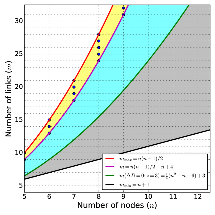
In summary, if a link community including 5 or more nodes is not separated only when it satisfies eq. 13 and does not have an independent triangle. If there is an independent triangle in a link community, it is always separated. If a link community is highly cliquish so that it satisfies eq. 14, it is always not separated. In conclusion, the condition where a community will not be broken into smaller chunks under partition density optimization is extremely limited, and the direct global optimization of partition density will result in mostly triangles with very few larger communities, failing to identify “communities” that are commonly conceptualized.
III Alternative optimization approaches
The clear limitation of partition density as a quality function for community detection is established. Thus, we seek alternative optimization approaches to identify link communities. Since link community (line graph) approach consists of (i) weighted line graph transformation Evans and Lambiotte (2009, 2010); Ahn et al. (2010); West et al. (2001) and (ii) clustering in the line graph space, we explore both the methods of weighted line graph transformation and other quality functions that can be optimized to identify disjoint communities in the transformed line graph.
The main rationale behind the weighted line graph transformation is to mitigate the problem that each hub becomes a huge clique by penalizing the connections between the links that are attached to the same hub. One approach to estimate the similarity between two links is based on preserving the dynamics of a random walker on the links of a network Evans and Lambiotte (2009, 2010). In this approach, if two links are connected via a node whose degree is , the weight of the corresponding link in the line graph becomes . We will call this approach a simple normalization scheme. Another approach is incorporating the information about the neighbors and ignoring the contribution from the shared node, by employing the Jaccard index Jaccard (1912); Ahn et al. (2010). In this approach, if we consider two links ( and ) that are attached to a hub , their similarity is entirely based on the neighbors of and , ignoring ’s neighbors. The similarity measure is defined as follows:
| (15) |
where is the set of the direct neighbors of node and itself Ahn et al. (2010). Compared to the simple normalization scheme, two distinct pairs of links connected via the same node can have different weights using the Jaccard index. In addition to the original Jaccard index, we introduce a normalized Jaccard index, which is the combination of the two above:
| (16) |
where is the degree of node . This similarity measure reduces the strength of cliques formed by hubs even further by not only incorporating the local information but also penalizing large hubs.
Once we generate line graphs based on the three aforementioned schemes, we can perform disjoint, node community detection on those weighted line graphs. As alternatives to partition density, we simply choose two of the most widely used quality functions: modularity and map equation (Infomap) Rosvall and Bergstrom (2008).
IV Experimental results
IV.1 Conformational space annealing (CSA) algorithm
We optimized partition density directly to show the preference of partition density toward triangles by using the conformational space annealing algorithm (CSA), which has been successfully applied to various global optimization problems Lee et al. (2003); Joo et al. (2008, 2009); Shin et al. (2011); Lee et al. (2011b, 2012); Sim et al. (2012); Joo et al. (2014, 2015). We converted the CSA implementation for modularity optimization Lee et al. (2012) to optimize partition density. Each solution is a -dimensional vector representing the community indices of links in a network. For local optimization of , we used a quench procedure, which accepts a move only when is improved, equivalent to simulated annealing at zero temperature. Detailed description on a general CSA algorithm can be found elsewhere Lee et al. (1997, 2012).
IV.2 Partition density optimization of synthetic networks
In this study, we used two classes of synthetic networks to show the limitation of partition density: Girvan-Newman (GN) Girvan and Newman (2002) and Lancichinetti-Fortunato-Radicchi (LFR) Lancichinetti and Fortunato (2009) benchmark networks. The GN benchmark network consists of 128 nodes divided into 4 node communities of 32 nodes. Each node is connected to the other nodes in the same community with links and to nodes in other modules with links. Every node has 16 links in total, . When , each node has more connections within the community than the rest of network and corresponds well to the four pre-defined communities. In the LFR network, the node degrees and community sizes are stochastically assigned to follow a power-law distribution. Links are stochastically connected based on a mixing parameter , ranging from 0 to 1. Each node shares a fraction of of links with the other nodes in the same community, and a fraction of of links with the rest of network. Thus, a community structure becomes weaker as increases, and a community structure in a strong sense exists until . In this study, GN networks are generated with values ranging from 4 to 12. LFR networks are generated with a degree distribution that follows a power-law distribution with an exponent of 2 ranging from 10 to 50. Community sizes are tuned to follow a power-law distribution with an exponent of 1 and ranges from 10 to 30.
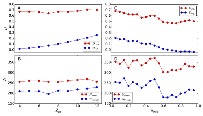
For the GN networks with different values ranging from 4 to 12, we compared optimized () values by CSA with the reference () value, which is obtained from the pre-defined node-community structure. To calculate the , all intra-node-community edges of a node-community are considered as the same link community and inter-node-community edges are ignored. For all GN networks, the values are much higher than the values (Figure 6A). The values are almost identical for all GN networks, around 0.7, while the value monotonically increases from 0.03 to 0.23 as the community structure of GN network strengthens. We also counted the numbers of triangles and all link communities from the CSA results (Figure 6B). For all the GN networks, around 260 link communities are detected via -optimization and, among them, around 220 link communities are triangles on average. In addition, it is noticeable that the number of triangle increases as increases, which suggests that highly modular networks may suffer more from this drawback of . These results show that the global optimization of leads to a significantly different community structure from the reference community due to the triangle preference of .
We performed a similar benchmark using LFR networks with different mixing probabilities. Overall, the benchmark on the LFR networks shows a qualitatively similar results with those on the GN networks. A comparison of and values demonstrates that there is a large gap between two values regardless of , and both values decrease as networks become less modular, a larger (Figure 6C). The inverse correlation between and shows that is correlated with the degree of modularity. However, as shown in the GN networks, community structures with high values does not correspond to the true community structure. From Figure 6D, it can be identified that about 2/3 of detected link communities via -optimization are triangles, and more triangles are detected in the networks with a strong sense of community, , than the networks without community, .
IV.3 Partition density optimization of real-world networks
We also performed -optimization of several popular real-world benchmark networks (Table. LABEL:tab:CSA_result_of_real_networks). For all real-world benchmark networks, more than half of detected link communities by -optimization are triangles, which indicates that the inverse resolution limit of partition density is universal. A comparison of the real groupings and the link communities obtained by -optimization of karate network is shown in Figure 7. In the real grouping, the karate network is divided into two and the value of the corresponding link community is 0.128 (Figure 7A). However, the CSA result with divides the karate network into 25 link communities, which includes 18 triangles and 4 unclassified edges (Figure 7B). There are two largest link communities consist of 6 edges connecting nodes 1-2-14-20-34 and 1-22-2-31-33-32, which mainly consist of hub nodes.
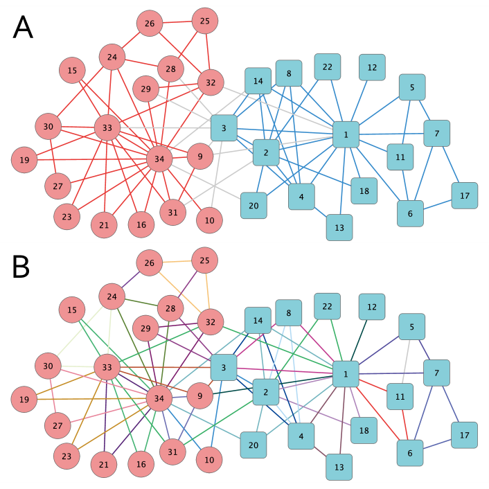
The results of the synthetic benchmark networks and the karate network give us a hint of how -optimization divides a network. -optimization finds as many cliques as possible because their local partition density, , is 1. Since the smallest clique is a triangle, most of edges are grouped as a triangle. After removing the detected cliques from the network, -optimization finds densely connected groups of the rest of edges, which are likely to be loosely connected groups of hub nodes due to their large degrees. The rest of disconnected edges remain unclassified, e.g. edges connecting 1-12 and 5-11 in Figure 7B.
| Dataset | # Triangle communities | # Communities |
|---|---|---|
| Karate | 18 | 25 |
| Dolphin | 30 | 51 |
| Lesmis | 26 | 44 |
| Political books | 83 | 120 |
| Football | 109 | 168 |
| Netscience_main | 98 | 200 |
| C. elegans | 297 | 512 |
| Jazz | 562 | 772 |
| E. coli | 1466 | 2184 |
IV.4 Modularity optimization of weighted line graphs
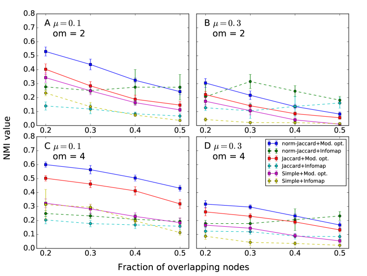
We used LFR benchmark networks for overlapping communities with 1000 nodes, mixing probabilities () of 0.1 and 0.3, and the numbers of memberships of an overlapping node (om) of 2 and 4 Lancichinetti and Fortunato (2009). With each parameter set, ten different networks were generated and tested. The qualities of community detection results were evaluated by calculating the normalized mutual information (NMI) values for overlapping communities Lancichinetti et al. (2009) between the obtained communities and the reference communities. Recently, it was reported that NMI is affected by the finite size of a network and the finite number of detected communities Zhang (2015). To remove this artifact, the NMI values are adjusted by subtracting the average NMI values of randomly shuffled communities while preserving the number of communities.
The benchmark results clearly show that performing community detection using the line graphs generated with the normalized Jaccard index yields the highest NMI values in most cases (Figure 8). With the modularity optimization method, the line-graphs generated with the normalized Jaccard index lead to higher NMI values for all parameter sets tested. With the the Infomap method, higher NMI values were consistently obtained with the normalize Jaccard index except two cases when line graphs are generated with the simple normalization scheme and , om=4, and the fraction of overlapping nodes are less than 0.4. In summary, these results indicate that detecting disjoint communities of the line graphs generated with the normalized Jaccard index leads to more meaningful link communities.
V Discussion and Conclusion
In this study, we showed that partition density suffers from the strong preference towards small cliques; identifying triangles as separate link communities is preferred in most possible scenarios. Direct global optimization of partition density of the synthetic and the real-world networks resulted in a huge number of triangles. We showed that a triangle contains a node that is connected only with the other two nodes, it always prefers to be separated. The only exception is when 4 nodes are connected with 5 links.
One of the reasons for the preference to a triangle is that a difference in local partition density between a triangle and larger cliques or cliquish link communities becomes marginal as a network becomes larger. By definition, a decrease in of a large link community due to a separation of a triangle becomes smaller as increases (eq. 1). However, of a separated triangle is 1.0, which can be larger enough to compensate the decreased of the initial link community. Our result raises further questions: how should we handle triangles? Is it more meaningful than a larger cliquish link community? Although a triangle is a clique, it may be too small to extract meaningful information from it and to reduce the complexity of a network efficiently. Thus, a criterion to compare the significance of a triangle and larger cliquish link communities may be necessary.
Considering the strong bias of the partition density how could it work as a quality function for the link clustering method Ahn et al. (2010)? First, a hierarchical clustering was performed in an agglomerative way to generate the dendrogram of links and detect the community structure of a network based on a threshold that maximizes partition density. With this approach, formation of triangles is suppressed because clustering is carried out in a way that the size of a cluster increases only by merging the most similar pair of nodes first, imposing strong constraints on the community structures. Second, the heterogeneity of a network might play an important role. If the degree distribution of nodes follows an uniform or a Gaussian distribution, many nodes may have similar numbers of links, direct neighbors, which makes most pairs of links have similar similarities. If this is the case, many triangles may have formed due to a high degeneracy of priorities of links for merging. However, many real-world networks are known to be scale-free networks whose degree distributions are highly heterogeneous. The heterogeneity of connectivity leads to a heterogeneous distribution of link similarities, which leads to the formation of the hierarchical organization of link communities Ahn et al. (2010).
As an alternative optimization approach to the partition density, we explored the possibilities of directly optimizing other quality functions combined with several versions of weighted line graph transformations. In the previous scheme suggested by Evans and Lambiotte, the weight of a link in a line-graph is set to the inverse of the degree of a common node Evans and Lambiotte (2009, 2010). This approach preserves the dynamics of random walkers. However, information on the similarities between links of an initial network is not reflected explicitly. Thus, this scheme may not be useful when one wants to investigate the relationships between links using a line-graph representation. In the previous link clustering study Ahn et al. (2010), the Jaccard index was used. We suggested the normalized Jaccard index, which combines these two previous approaches. Modularity optimization of the line-graphs generated with the normalized Jaccard index resulted in more accurate community structures than those with the Jaccard index or the simple normalization scheme alone, prompting further investigation into good quality functions and weighting schemes for line-graph based link community detection.
Acknowledgements.
YYA thanks for the support from Microsoft Research Faculty Fellowship.References
- Fortunato (2010) S. Fortunato, Phys. Rep. 486, 75 (2010).
- Newman and Girvan (2004) M. Newman and M. Girvan, Phys. Rev. E 69, 1 (2004).
- Lee et al. (2012) J. Lee, S. P. Gross, and J. Lee, Phys. Rev. E 85, 056702 (2012).
- Zhang et al. (2009) X. Zhang, R. Wang, Y. Wang, J. Wang, Y. Qiu, L. Wang, and L. Chen, Europhys. Lett 87, 38002 (2009).
- Bagrow (2012) J. P. Bagrow, Phys. Rev. E 85, 066118 (2012).
- Lee and Lee (2013) J. Lee and J. Lee, PLoS ONE 8, e60372 (2013).
- Lee et al. (2013) J. Lee, S. P. Gross, and J. Lee, Sci. Rep. 3, 2197 (2013).
- Good et al. (2010) B. H. Good, Y.-A. de Montjoye, and A. Clauset, Phys. Rev. E 81, 046106 (2010).
- Fortunato and Barthelemy (2007) S. Fortunato and M. Barthelemy, Proc. Nat. Acad. Sci. USA 104, 36 (2007).
- Palla et al. (2005) G. Palla, I. Derényi, I. Farkas, and T. Vicsek, Nature 435 (2005).
- Ahn et al. (2010) Y.-Y. Ahn, J. P. Bagrow, and S. Lehmann, Nature 466, 761 (2010).
- Lee et al. (2011a) S. H. Lee, P.-J. Kim, and H. Jeong, BMC Syst. Biol. 5, 1 (2011a).
- Malik et al. (2014) A. Malik, J. Lee, and J. Lee, PLoS ONE 9, e95480 (2014).
- Lancichinetti et al. (2009) A. Lancichinetti, S. Fortunato, and J. Kertész, New J. Phys. 11, 033015 (2009).
- Evans and Lambiotte (2010) T. S. Evans and R. Lambiotte, Eur. Phys. J. B 77, 265 (2010).
- Viamontes Esquivel and Rosvall (2011) A. Viamontes Esquivel and M. Rosvall, Phys. Rev. X 1, 021025 (2011).
- Lancichinetti et al. (2011) A. Lancichinetti, F. Radicchi, J. J. Ramasco, and S. Fortunato, PLoS ONE 6, e18961 (2011).
- Yang and Leskovec (2012) J. Yang and J. Leskovec, Proc. IEEE Int. Conf. Data Min. 1, 1170 (2012).
- Xie et al. (2013) J. Xie, S. Kelley, and B. K. Szymanski, ACM Comput. Surv. 45, 1 (2013), arXiv:1110.5813 .
- Gopalan and Blei (2013) P. K. Gopalan and D. M. Blei, Proc. Nat. Acad. Sci. USA 110, 14534 (2013).
- Zhang et al. (2013) Z.-Y. Zhang, Y. Wang, and Y.-Y. Ahn, Phys. Rev. E 87, 062803 (2013).
- West et al. (2001) D. B. West et al., Introduction to Graph Theory, Vol. 2 (Prentice hall Upper Saddle River, 2001).
- Evans and Lambiotte (2009) T. S. Evans and R. Lambiotte, Phys. Rev. E 80, 016105 (2009).
- Jaccard (1912) P. Jaccard, New Phytol. XI, 37 (1912).
- Rosvall and Bergstrom (2008) M. Rosvall and C. T. Bergstrom, Proc. Nat. Acad. Sci. USA 105, 1118 (2008).
- Lee et al. (2003) J. Lee, I.-H. Lee, and J. Lee, Phys. Rev. Lett. 91, 080201 (2003).
- Joo et al. (2008) K. Joo, J. Lee, I. Kim, S. J. Lee, and J. Lee, Biophys. J. 95, 4813 (2008).
- Joo et al. (2009) K. Joo, J. Lee, J.-H. Seo, K. Lee, B.-G. Kim, and J. Lee, Proteins: Struct., Funct., Bioinf. 75, 1010 (2009).
- Shin et al. (2011) W.-H. Shin, L. Heo, J. Lee, J. Ko, C. Seok, and J. Lee, J. Comput. Chem. 32, 3226 (2011).
- Lee et al. (2011b) J. Lee, J. Lee, T. N. Sasaki, M. Sasai, C. Seok, and J. Lee, Proteins: Struct., Funct., Bioinf. 79, 2403 (2011b).
- Sim et al. (2012) S. Sim, J. Lee, and J. Lee, (2012), arXiv:1209.0549 .
- Joo et al. (2014) K. Joo, J. Lee, S. Sim, S. Y. Lee, K. Lee, S. Heo, I.-H. Lee, S. J. Lee, and J. Lee, Proteins: Struct., Funct., Bioinf. 82 Suppl 2, 188 (2014).
- Joo et al. (2015) K. Joo, I. Joung, S. Y. Lee, J. Y. Kim, Q. Cheng, B. Manavalan, J. Y. Joung, S. Heo, J. Lee, M. Nam, I.-H. Lee, S. J. Lee, and J. Lee, Proteins: Struct., Funct., Bioinf. , n/a (2015).
- Lee et al. (1997) J. Lee, H. A. Scheraga, and S. Rackovsky, J. Comput. Chem. 18, 1222 (1997).
- Girvan and Newman (2002) M. Girvan and M. E. Newman, Proc. Nat. Acad. Sci. USA 99, 7821 (2002).
- Lancichinetti and Fortunato (2009) A. Lancichinetti and S. Fortunato, Phys. Rev. E 80, 016118 (2009).
- Zhang (2015) P. Zhang, (2015), arXiv:1501.0384 .