remarkRemark \newsiamremarkhypothesisHypothesis \newsiamthmclaimClaim \headersNon-smooth Variable ProjectionT. van Leeuwen and A. Aravkin
Variable Projection for non-smooth problems††thanks: Submitted to the editors June 29, 2020.
Abstract
Variable projection solves structured optimization problems by completely minimizing over a subset of the variables while iterating over the remaining variables. Over the last 30 years, the technique has been widely used, with empirical and theoretical results demonstrating both greater efficacy and greater stability compared to competing approaches. Classic examples have exploited closed-form projections and smoothness of the objective function. We extend the approach to problems that include non-smooth terms, and where the projection subproblems can only be solved inexactly by iterative methods. We propose an inexact adaptive algorithm for solving such problems and analyze its computational complexity. Finally, we show how the theory can be used to design methods for selected problems occurring frequently in machine-learning and inverse problems.
keywords:
variable projection, inexact proximal gradient68Q25, 68R10, 68U05
1 Introduction
In this paper we consider finite-dimensional separable optimization problems of the form
| (1) |
where smoothly couples but may be non-convex, while and encode additional constraints or regularizers. We are particularly interested in the case where is strongly convex in , so that fast solvers are be available for optimizing over for fixed . These problems arise any time non-smooth regularization or constraints are used to regularize certain difficult non-linear inverse problems or regression problems. We give three motivating examples below.
1.1 Motivating examples
Model calibration
Consider the non-linear fitting problem
| (2) |
where defines a linear model with calibration parameters and denotes the data. Well-known examples include exponential data-fitting and model-calibration in inverse problems. Adding regularization terms immediately gives a problem of the form Eq. 1.
Machine learning
Trimming is a model-agnostic tool for guarding against outliers. Given any machine learning model that minimizes some objectives over a training set of datapoints, we introduce auxiliary parameters that serve to distinguish inliers from outliers and solve
where is the number of datapoints we want to fit. The functions can capture a wide range of machine learning models.
PDE-constrained optimization
Many PDE-constrained optimization problems in data-assimilation, inverse problems and optimal control can be cast as
where denotes the state of the system, is the sampling operator, is the discretized PDE with coefficients and source term , and is a penalty parameter. Adding regularization terms or changing the data-fidelity term gives a problem of the form Eq. 1.
1.2 Approach
The development of specialized algorithms for (1) goes back to the classic Variable Projection (VP) technique for separable non-linear least-squares problems of the form (2), where the matrix-valued map is smooth and the matrix has full rank for each . Early work on the topic, notably by [8] has found numerous applications in chemistry, mechanical systems, neural networks, and telecommunications. See the surveys of [9] and [10], and references therein.
The VP approach is based on eliminating the variable , as for each fixed we have a closed-form solution
where denotes the Moore-Pensrose pseudo-inverse of . We can thus express (2) in reduced form as
| (3) |
which is a non-linear least-squares problem. Note that is an orthogonal projection onto the null-space of ; hence the name variable projection.
It was shown by [8] that the Jacobian of contains only partial derivatives of w.r.t. and does not include derivatives of w.r.t. . [14] showed that when the Gauss-Newton method for (2) converges superlinearly, so do certain Gauss-Newton variants for (3). Numerical practice shows that the latter schemes actually outperform the former on the account of a better conditioning of the reduced problem.
The underlying principle of the VP method is much broader than the class of separable non-linear least squares problems. For example, [5, 2] consider the class of problems
| (4) |
where is a -smooth function; the classic VP problem (2) is a special case of (4). Although we generally do not have a closed-form expression for , we define it as
and express (4) using the projected function
| (5) |
Projection in the broader context of (4) refers to epigraphical projection [12], or partial minimization of . Under mild conditions, is -smooth as well and its gradient is given by
| (6) |
i.e., it is the gradient of w.r.t. , evaluated at [5]. Again, we do not need to compute any sensitivities of w.r.t. . This is seen by formally computing the gradient of using the chain-rule:
| (7) |
Since is a minimizer of it satisfies and the second term vanishes. Similarly, the Hessian of is the Schur complement of of the full Hessian of [14]:
| (8) |
It follows that a local minimizer, , of together with constitute a local minimizer of . An interlacing property of the eigenvalues of the Schur complement can be used to show that the reduced problem has a smaller condition number than the original problem [17]. The expression for the derivative furthermore suggests that we can approximate the gradient of when is known only approximately by ignoring the second term.
We may extend this approach to solve problems of the form (1) by including in the computation of and using an appropriate algorithm to minimize . Define the proximity operator for any function as follows:
where is any scaling factor or stepsize. We can now view the entire approach as proximal-gradient descent on the projected function
| (9) |
where is an appropriate step and is computed using (6). This gives rise to the following protype algorithm 1.
Naively, this approach can be applied to non-smooth problems; however, it is not immediately obvious that it is guaranteed to converge. In particular, the resulting reduced objective may not be smooth and hence the gradient formula (6) may not be valid. This is illustrated in the following example.
Examples
To illustrate the possibilities and limitation for extending the VP approach to non-smooth functions, consider the following functions
The corresponding and are shown in figure Fig. 1. For cases 1 - 3, is continuous (but not smooth), leading to a smooth projected function. For , is not continuous (at the solution is not unique), leading to a non-smooth projected function. Continuity of thus appears to be important, rather than smoothness of in . We therefore restrict our attention to problems of the form Eq. 1 that are strongly convex in for all of interest.


The goal of this paper is to extend the variable projection technique to problems of the form (1) with non-smooth regularization terms, which arise in high-dimensional statistics, signal processing, and many machine learning problems; sparse regularization and simple constraints are frequently used in this setting.
1.3 Contributions and outline
Our contributions are as follows:
2 Derivative Formulas and Inexact VP
In this section, we present derivative formulas and develop the approaches briefly described in the introduction. The proofs of the following statements are found in the appendix. By we denote the Euclidean norm. We make the following blanket assumptions on and :
- A1
-
and exist and are Lipschitz-continuous for all :
- A2
-
is -strongly convex in for all .
2.1 Derivative formulas
We first establish Lipschitz continuity of the solution w.r.t. in the following Lemma.
Lemma 2.1.
Let satisfy assmptions (A1-A2), then is Lipschitz-continuous as a function of :
Next, we establish that the naive derivative-formula Eq. 7 holds under the aforementioned assumptions.
Theorem 2.2.
Let satisfy assmptions (A1-A2) and define . The gradient of the projected function is then given by , with .
Finally, we establish Lipschitz continuity of the gradient of the projected function.
Corollary 2.3.
The gradient of is Lipschitz continuous:
where
Remark 2.4.
Note that the bound in Corollary 2.3 is consistent with the expression for the Hessian in Eq. 8 in the smooth case.
These results immediately establish the convergence of Algorithm 1 to a stationary point for a broad class of problems of the form Eq. 1.
2.2 Inexactness
In many applications, we do not have a closed-form expression for and it must be computed with an iterative scheme. An obvious choice is to use a proximal gradient method
with . The resulting approximation, , of yields an approximation of the gradient of with error
This gives rise to an inexact counterpart of (9):
| (10) |
with . We denote the error in the gradient as . We can immediately bound this error as
| (11) |
Conditions under which such iterations converge in case is (strongly) convex have been well-studied [7, 15]. The basic gist of these results is that convergence of Eq. 10 can be ensured when the error decays sufficiently fast with .
We did not find any results for general in the literature and therefore establish convergence of the inexact prox-gradient method for general Lipschitz-smooth in the following theorem.
Theorem 2.5 (Convergence of inexact proximal gradient - general case).
Denote
and let be the Lipschitz constant of . The iteration
| (12) |
using stepsize and with errors obeying with produces iterates for which
with .
The proof of this theorem along with supporting Lemma’s are presented in Appendix D. This result immediately establishes convergence of Eq. 10 for problems satisfying assumptions (A1-A2) when the errors in the gradient obey . We discuss how to ensure this in practice in a subsequent section.
Stronger statements on the rate of convergence can be made by making stronger assumptions about . When is convex (i.e., when is jointly convex in ), a sublinear convergence rate of can be ensured when for any [15, Prop. 1]. A linear convergence for strongly convex can be ensured when for any [15, Prop. 3].
2.3 Asymptotic complexity
In this section we analyse the asymptotic complexity of finding an -optimal estimate of the solution to Eq. 1 which satisfies
We measure the complexity in terms of the total number of inner iterations required to achieve this. To usefully analyse the asymptotic complexity we assume that is (strongly) convex.
We first note that we can produce an -optimal estimate of for which in inner iterations. This follows directly from linear convergence of the proximal gradient method for strongly convex problems. This also implies that we can compute an approximation of the gradient of with error bounded by in inner iterations.
- Convex case
-
To achieve sublinear convergence of the outer iterations for convex , we need for any [15, Prop. 1]. To achieve this we need to decrease the inner tolerance at the same rate; . Due to linear convergence of the inner iterations, this requires inner iterations. A total of outer iterations thus has an asymptotic complexity of . Due to sublinear convergence of the outer iterations, we require outer iterations, giving a complexity of .
- Strongly convex case
-
To achieve linear convergence of the outer iterations for strongly convex , we need for any [15, Prop. 3]. To achieve this we need to decrease the inner tolerance at the same rate; . Due to linear convergence of the inner iterations, this requires inner iterations. A total of outer iterations then require inner iterations. Due to linear convergence of the outer iterations, we require outer iterations, giving an overall complexity of .
2.4 Practical implementation
A basic proximal gradient method for solving problems of the form Eq. 1 is shown in Algorithm 2, where we denote
The conventional VP algorithm with accurate inner solves is given in Algorithm 3. By Lemma E.1 the stopping criterion for the inner iterations guarantees that at outer iteration , we have and hence that the error in the gradient is bounded by
We use warmstarts for the inner iterations, which is expected to dramatically reduce the required number of inner iterations, especially when getting close to the solution.
An inexact version of Algorithm 3 can be implemented by specifying a decreasing sequence of tolerances . However, in practice it would be hard to figure out exactly how fast to decrease the tolerance. Inspired by the requirement for convergence of the inexact proximal gradient method we therefore propose a stopping criterion based on the progress in the outer iterations. Theorem 2.5 requires that the error in the gradient is bounded by . We can guarantee this by combining various bounds. By Eq. 11 and Lemma E.1 we get
which guarantees the required bound on the error. Note that implicitly depends on and through .
A practical implementation of the inexact method is shown in Algorithm 4. In practice the constants and may difficult to estimate. Moreover, the bounds may be very loose. We therefore introduce a parameter, , to use in the stopping criterion instead.
In particular settings, the structure of the inner problem in can be exploited to achieve superlinear convergence of the inner iterations. A further improvement could be to use a line search or an accelerated proximal gradient method for the outer iterations. However, accelerated proximal gradient methods are generally more sensitive to errors or require more information on the function, as pointed out by [15].
3 Case studies
3.1 Reproducibility
The Python code used to conduct the numerical experiments is available at https://github.com/TristanvanLeeuwen/VarProNS. We implemented Algorithm 2 (hereafter referred to as the joint approach), Algorithm 3 (VP) and Algorithm 4 (adaptive VP). In stead of the absolute tolerance for the inner iterations in Algorithm 3 we use a relative tolerance and stop the inner iterations in Algorithm 3 when . For the outer iterations we use a stopping criterion on the function value. The Lipschitz constants , and other algorithmic parameters are specified for each example. We show results for several values of to investigate the sensitivity of the results to this parameter.
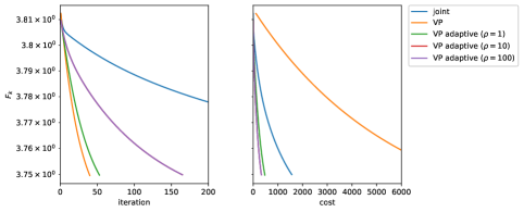
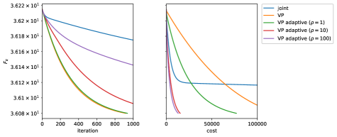
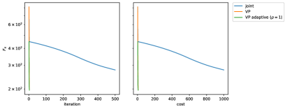
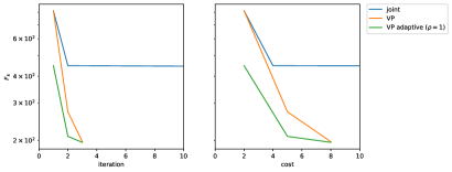
Aside from the example-specific results, we report the convergence history (in terms of the value of the objective) as a function of the number of outer iterations and the total number of iterations. The latter is used as an indication of the computational cost, and will be referred to as cost.
3.2 Exponential data-fitting
We begin with the general class of exponential data-fitting problems – one of the prime applications of variable projection [11]. The general formulation of these problems assumes a model of the form
where are unknown weights, are the measurements, and are given functions that depend on an unknown parameter . Some examples of this class are given in table 1.
| application | |
|---|---|
| pharmaco-kinetic modelling | |
| multiple signal classification | |
| radial basis function interpolation |
The exponential data-fitting problem is traditionally formulated as a least-squares problem
In many applications, however, it is natural to include regularization terms and/or use another data fidelity term. For example, [6, 16] consider positivity constraints . Another common regularization that enforces sparsity of is . This is useful in cases where the system is over-parametrized and we are looking for a fit of the data with as few components as possible. Even with regularization, we expect a highly ill-posed problem where many parameter combinations lead to a nearly identical data-fit.
For the conditions of the previous theorems to hold we require to be invertible for all . Note that this would require for . As long as we initialize the to be different, we don’t expect any problems. Alternatively, a small quadratic term in could be added to ensure that is strongly convex in .
3.2.1 Example 1
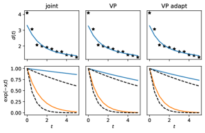
We model the data via a normal distribution with mean and variance . To generate the data, we set , , , , and . Since the number of components, , is not typically known in practice, we attempt the fit the data using components and use an -regularization term with (chosen by trial and error) to find a parsimonious solution. The variational problem is then given by
Here, is an matrix with elements . The Lipschitz-constants of and are set to (selected by trial and error). For the inner solves we let (for the true ), for VP and for adaptive VP. With these settings we run Algorithm 2 (joint), Algorithm 3 (VP) and Algorithm 4 (adaptive VP). The results are shown in Fig. 2 and Fig. 3. The VP approach gives a slightly better recovery of the modes while achieving the same level of data-fit as the joint approach. This indicates that the ill-posedness of the problem is effectively dealt with by the VP approach. The VP approach converges much faster than the joint approach. While the exact VP approach is much more expensive than the joint approach, the adaptive VP method is much cheaper than the joint approach.
3.2.2 Example 2
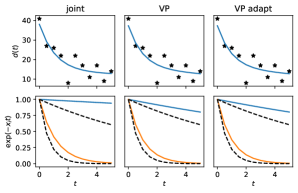
Here, we model the data via a Poisson distribution with parameter . We set , , , , . The other settings are exactly the same as the previous example. The variational problem is now given by
where denotes the Poisson log-likelihood function. The Lipschitz-constants of and are set to (selected by trial and error). For the inner solves we let (for the true ), for inexact VP and for adaptive VP. With these settings we run Algorithm 2 (joint), Algorithm 3 (VP) and Algorithm 4 (adaptive VP). The results are shown in Fig. 5 and Fig. 4. Here again the VP approach gives a slightly better recovery of the modes while achieving the same level of data-fit as the joint approach. This indicated the ill-posedness of the problem that is effectively dealt with by the VP approach. The VP approach converges much faster than the joint approach. The adaptive VP method is (much) cheaper than the joint approach and even the regular VP approach eventually beats the joint approach.
3.3 Trimmed Robust Formulations in Machine Learning
Many formulations in high-dimensional regression, machine learning, and statistical inference can be formulated as minimization problems
where the training set comprises examples and is the error or negative log-likelihood corresponding to the th training point. This approach can be made robust to perturbations of input data (for example, incorrect features, gross outliers, or flipped labels) using a trimming approach. The idea, first proposed by [13] in the context of least squares fitting, is to minimize the best residuals. The general trimmed approach, formulated and studied by [20], considers the equivalent formulation
where denotes the capped simplex and admits an efficient projection [19, 1]. Jointly solving for selects the inliers as the model is fit. Indeed, the reader can check that the solution in for fixed selects the smallest terms . The problem therefore looks like a good candidate for VP, but the projected function is nonsmooth, because the solution for may not be unique111Consider, for example, a case where a number of residuals have the same value.. However, the smoothed formulation
| (13) |
does lead to a differentiable as the problem is now strongly convex in .
To illustrate the trimming method and the potential benefit of the VP approach we consider the following stylized example.
3.3.1 Example 1
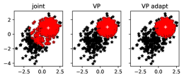
We aim to compute the (trimmed) mean of a set of samples by setting . We generate data by sampling generating a total of samples ; are drawn from a normal distribution with mean and variance while the remaining are drawn from a normal distribution with mean and variance . We let , and , for VP and for adaptive VP. The results for Algorithm 2 (joint), Algorithm 1 (VP), Algorithm 4 (adaptive VP) are shown in figures Fig. 6 and Fig. 7. We note that the VP approach gives a better recovery of the inliers. Moreover, the VP approach converges much faster than the joint approach. As the inner problem is a simple quadratic, both the exact and adaptive VP approach have essentially the same computational cost.
3.4 Tomography
In computed tomography (CT) the data consists of a set of line integrals of an unknown function
where represents a line with angle and offset . Collecting measurements for angles , offsets and representing the function as a piecewise continuous function on a grid of rectangular pixels leads to a system of linear equations , with , with representing the gray value of the image in the pixel. In many applications, the angles and absolute offsets are not known exactly due to calibration issues. To model this we include additional parameters for each angle. This leads to the following signal model
where contains the calibration parameters and represents measurement noise222In low-dose applications, a Poisson noise model is more realistic.. We can ensure that depends smoothly on by using higher-order interpolation [18]. Many alternative methods have been proposed to solve the calibration problem [18, 3] and we do not claim that the proposed VP approach is superior; we merely use this problem as an example to compare the joint, VP and adaptive VP approaches amongst each other.
3.4.1 Example 1
We let , and take offsets regularly sampled in and angles regularly sampled in . This does not guarantee an invertible Hessian (e.g., strongly convex ) for all , however, we will see that this does not lead to numerical issues in this particular example. As a safeguard, one could add a small quadratic regularizer to the objective.
The data are generated with an additional random perturbation on the offset and angles (both are normally distributed with zero mean and variance ) and measurement noise (normally distributed with zero mean and variance ).
To regularize the problem we include positivity constraints:
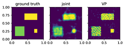
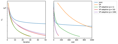
For the optimization we let and (for the true ), for VP and for adaptive VP. With these settings we run Algorithm 2 (joint), Algorithm 3 (VP) and Algorithm 4 (adaptive VP). The results are shown in Fig. 8. The VP approach gives a much better reconstruction than the joint approach, owing to the much faster convergence. The adaptive VP methods are cheaper than the joint method, again because they converge much faster. The adaptive VP approach, in turn, is much cheaper than the exact VP approach.
3.4.2 Example 2
The settings are the same as in the previous example, except that we use a TV-regularization term:
with
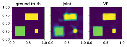
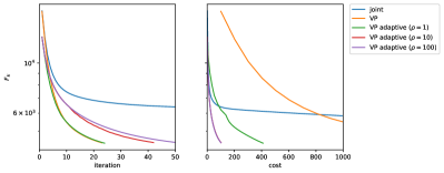
where returns a finite-difference approximation of the first derivative of the image in the direction. We let (chosen by trial and error). The results are shown in Fig. 9. The VP approach gives a much better reconstruction than the joint approach, owing to the much faster convergence. Both exact and adaptive VP are cheaper than the joint method, again because they converge much faster. The adaptive VP approach, in turn, is much cheaper than the exact VP approach.
4 Conclusions
Variable projection has been successfully used in a variety of contexts; the popularity of the approach is largely due to its superior numerical performance when compared to joint optimization schemes. In this paper, we extent its use to wide class of non-smooth and constrained problems occurring in various applications. In particular, we give sufficient conditions for the applicability of an inner-outer proximal gradient method. We also propose an inexact algorithm with an adaptive stopping criterion for the inner iterations and show that it retains the same convergence rate as the exact algorithm. Numerical examples on a wide range of nonsmooth applications show that: i) the variable projection approach leads to faster convergence than the joint approach, and ii) the adaptive variable projection method outperforms both the joint method and exact variable projection method in terms of computational cost. The adaptive method includes a parameter, , that controls the stopping tolerance for the inner iterations. In the numerical experiments we observe that a larger value for leads to a smaller number of outer iterations. There appears to be little danger of setting too large; even when varying it over two orders of magnitude the adaptive VP method is consistently faster than the exact VP method. As , the adaptive method coincides with the exact method. Heuristics could be developed to set this parameter automatically, but since this will be highly application-specific, it is outside the scope of this paper.
Appendix A Proof of Lemma 2.1
Proof A.1.
Denote . For ease of notation we fix and denote the corresponding (unique) optimal solutions by and respectively. These optimal solutions are implicitly defined by the first order optimality conditions and , or equivalently
| (14) |
We start from strong convexity of . For any we have
| (15) |
with and . We note that so we can write
with (15) holding for any choice of and . Using (14), we make the particular choices and . From (15) we now have
Setting , we get
Finally, using Cauchy-Schwartz and Lipschitz-smoothness of in we have
Appendix B Proof of Theorem 2.2
Proof B.1.
We set out to show that
| (16) |
which would confirm that is indeed the gradient of .
Using the definition of we rewrite (16) as
Writing with for , we get
| (17) |
We now set out to bound the terms in the numerator of Eq. 17 in terms of :
-
•
For the gradient terms we get (by Cauchy-Schwartz):
Furthermore, by Lipschitz continuinty of we have
Using that and Lipschitz continuity of (Lemma 2.1) we find
This results in
-
•
Next, we need to bound in terms of . Since is the optimal solution at we have . Using the convexity of we have
with . This can be expressed as with . Choosing appropriately as we get
Using Lipschitz continuity of and we get
We have thus upperbounded the term in Eq. 17 in terms of . As this upper bound tends to zero as and the fraction is always nonnegative we conclude that the limit tends to zero.
Appendix C Proof of Corollary 2.3
Proof C.1.
For ease of notation we fix and denote the corresponding (unique) optimal solutions by and respectively. Using the definition we have
Using Lipschitz continuity of and we immediately find
Appendix D Proximal gradient with errors
Consider solving
with , where is proper, closed and Lipschitz smooth and proper closed and convex. We consider an inexact proximal gradient method of the form
| (18) |
For the following we closely follow [4].
Lemma D.1 (Sufficient decrease of inexact proximal gradient).
Proof D.2.
By the smoothness assumption we have
By [4, Thm. 6.39] we have
which yields
Combining gives the result.
We let and state a simple corollary that ensures that we can get descent if is small enough.
Corollary D.3 (Existence of small enough errors).
At any iterate, we can always take small enough to ensure descent, unless is a stationary point.
Proof D.4.
Introduce the prox-gradient mapping :
If is non-stationary, we know that is bounded away from . On the other hand, the function
is -Lipschitz continuous, since the norm and the prox map are both 1-Lipschitz continuous, and we have and . Therefore, if we take , we have
and therefore
So if we take , we are guaranteed that , ensuring descent by Lemma D.1.
Theorem D.5 (Convergence of inexact proximal gradient - general case).
Appendix E A stopping criterion for prox gradient descent
When solving
where is Lipschitz-smooth and is strongly convex, with a proximal gradient method, we need a practical stopping criterion that can guarantee a certain distance to the optimal solution. The following bound is usefull:
Lemma E.1 (A stopping criterion for proximal gradient descent).
Introduce the prox-gradient mapping and the gradient mapping, :
where is Lipschitz-smooth and strongly convex, is convex and . Define the fixed point of by . Then,
Proof E.2.
By strong convexity of we have
with . Note that and that
by definition of the proximal operator. Picking this particular element in we obtain
By Lipschitz-smoothness and Cauchy-Schwartz we get
Remark E.3.
When applying a standard proximal gradient method we can immediately use this bound to devise a stopping criterion that guarantees .
References
- [1] Aleksandr Aravkin and Damek Davis. A smart stochastic algorithm for nonconvex optimization with applications to robust machine learning. arXiv preprint arXiv:1610.01101, 2016.
- [2] Aleksandr Y. Aravkin and Tristan van Leeuwen. Estimating nuisance parameters in inverse problems. Inverse Problems, 28(11):115016, nov 2012.
- [3] Anthony P. Austin, Zichao Wendy, Sven Leyffer, and Stefan M. Wild. Simultaneous Sensing Error Recovery and Tomographic Inversion Using an Optimization-Based Approach. SIAM Journal on Scientific Computing, 41(3):B497–B521, jan 2019.
- [4] Amir Beck. First-Order Methods in Optimization. Society for Industrial and Applied Mathematics, 2017.
- [5] B.M. Bell and J.V. Burke. Algorithmic differentiation of implicit functions and optimal values. In Christian H. Bischof, H. Martin Bücker, Paul D. Hovland, Uwe Naumann, and J. Utke, editors, Advances in Automatic Differentiation, pages 67–77. Springer, 2008.
- [6] Anastasia Cornelio, E. Loli Piccolomini, and J. G. Nagy. Constrained variable projection method for blind deconvolution. In Journal of Physics: Conference Series, volume 386, pages 6–11, 2012.
- [7] Olivier Devolder, François Glineur, and Yurii Nesterov. First-order methods of smooth convex optimization with inexact oracle. Mathematical Programming, 146(1-2):37–75, 2014.
- [8] G.H. Golub and V. Pereyra. The differentiation of pseudo-inverses and nonlinear least squares which variables separate. SIAM J. Numer. Anal., 10(2):413–432, 1973.
- [9] G.H. Golub and V. Pereyra. Separable nonlinear least squares: the variable projection method and its applications. Inverse Problems, 19(2):R1, 2003.
- [10] M.R. Osborne. Separable least squares, variable projection, and the Gauss-Newton algorithm. Electronic Transactions on Numerical Analysis, 28(2):1–15, 2007.
- [11] V. Pereyra and G. Scherer, editors. Exponential Data Fitting and its Applications. Bentham Science and Science Publishers, mar 2012.
- [12] R.T. Rockafellar and R.J.B. Wets. Variational Analysis, volume 317. Springer, 1998.
- [13] P. J Rousseeuw. Least Median of Squares Regression. Journal of the American statistical association, 79(388):871–880, 1984.
- [14] A. Ruhe and P.A. Wedin. Algorithms for separable nonlinear least squares problems. SIAM Rev., 22(3):318–337, 1980.
- [15] Mark Schmidt, Nicolas L Roux, and Francis R Bach. Convergence rates of inexact proximal-gradient methods for convex optimization. In Advances in neural information processing systems, pages 1458–1466, 2011.
- [16] Paul Shearer and Anna C Gilbert. A generalization of variable elimination for separable inverse problems beyond least squares. Inverse Problems, 29(4):045003, apr 2013.
- [17] Ronald L. Smith. Some interlacing properties of the Schur complement of a Hermitian matrix. Linear Algebra and its Applications, 177:137–144, 1992.
- [18] Tristan van Leeuwen, Simon Maretzke, and K Joost Batenburg. Automatic alignment for three-dimensional tomographic reconstruction. Inverse Problems, 34(2):024004, feb 2018.
- [19] Weiran Wang and Canyi Lu. Projection onto the capped simplex. arXiv preprint arXiv:1503.01002, 2015.
- [20] Eunho Yang, Aurélie C Lozano, Aleksandr Aravkin, et al. A general family of trimmed estimators for robust high-dimensional data analysis. Electronic Journal of Statistics, 12(2):3519–3553, 2018.