Parameter fitting in three-flavor Nambu–Jona-Lasinio model
with various regularizations
Abstract
We study the three-flavor Nambu–Jona-Lasinio model with various regularization procedures. We perform parameter fitting in each regularization and apply the obtained parameter sets to evaluate various physical quantities, several light meson masses, decay constant and the topological susceptibility. The model parameters are adopted even at very high cutoff scale compare to the hadronic scale to study the asymptotic behavior of the model. It is found that all the regularization methods except for the dimensional one actually lead reliable physical predictions for the kaon decay constant, sigma meson mass and topological susceptibility without restricting the ultra-violet cutoff below the hadronic scale.
HUPD-1511
1 Introduction
Nonet mesons are interesting composite hadronic objects which have been seriously studied in theoretical and experimental particle physics. The elementary objects composing mesons are quarks and gluons, and the first principle theory of them is quantum chromodynamics (QCD). Then one of our goals is to explain all the information on hadrons from QCD. The most reliable approach is to consider the discretized version of QCD, called the lattice QCD, whose technologies are developing day by day. It is, however, still difficult to study hadrons from the first principle, so the approaches by using some effective models become one of our options.
In this paper we employ the Nambu–Jona-Lasinio (NJL) model [1] being one of frequently used models for the investigations of hadronic particles. The three-flavor model with anomaly [2] called Kobayashi–Maskawa–’t Hooft (KMT) term [3] successfully describes the nonet meson properties (for reviews, see, e.g., [4, 5, 6, 7, 8, 9]). The model is not renormalizable, since it contains the higher dimensional operators, four- and six-point fermion interactions. Therefore the model predictions inescapably depend on the regularization procedures. Also, the model shows parameter dependence in each regularization method. Then we have launched a plan to perform the systematical analyses on both the regularization and parameter dependence.
Here we are going to study the model with five regularizations: the three-dimensional (3D) and four-dimensional (4D) sharp cutoff schemes, Pauli-Villars (PV), the proper-time (PT) and the dimensional regularizations (DR), as the straightforward extension of the work with the two-flavor model [10]. The 3D cutoff drops the higher momentum contribution in the space direction, which is the most frequently used method due to its simple physical interpretation and nice numerical behavior. Similarly, the 4D cutoff method kills the amplitudes from higher momentum in the four-dimensional Euclidean momentum space. The PV way reduces high momentum contribution by subtracting the amplitudes from virtual heavy particles [11, 12, 13]. The PT method introduces the exponentially dumping factor in the integral, then make divergent loop integrals finite [12, 14]. The DR prescription modifies an integral kernel through changing the space-time dimension so as to make divergent integrals finite. The model has been examined in detail with various regularizations, see, e.g., for the 4D [5, 6, 15, 16, 17], PV [5, 18, 19, 20, 21], PT [22, 23, 24, 25, 26, 27, 28, 29] and DR [15, 16, 17, 31, 32, 33, 34, 35, 36]. The NJL model is regarded as a low energy effective model of QCD; it is the simplest model to induce dynamical chiral symmetry breaking and often applied to investigate physics near the QCD phase transition. To apply the model to the nonet mesons and mesons may be not light enough compared with the QCD scale. Since the model loses validity at higher energy, it should be essential to evaluate the safety and effectiveness of the model with the regularization procedures. It is to be noted that the model has non-negligible parameter dependence even within the same regularization procedure [10]. In particular, some physical quantities, such as the transition temperature on the chiral symmetry breaking, are crucially affected by the model parameters. Moreover, there exists some room for the choice of parameters since input physical quantities for setting the parameters are usually less than the number of the parameters, then several parameter sets are employed depending on working groups [6, 7, 15, 20, 29]. Therefore it is also important to test the parameter dependence on the model predictions. A lot of works have been devoted to the searches on the model parameters with various regularizations. For the sake of seeing the regularization and parameter dependence on the physical quantities, in this article, we shall perform the systematical parameter fitting in the three flavor model.
The paper is constructed as follows: Section 2 presents the model treatments and the regularization procedures. We will carry on the detailed parameter fitting in Sec. 3. Section 4 is devoted to the investigations on the physical predictions. We give some discussions on the parameter fitting in Sec. 5. Some concluding remarks are put in Sec. 6. Appendix shows the explicit equations for the meson properties and topological susceptibility.
2 Model and regularizations
We start from the model Lagrangian then derive the effective potential and the gap equations in the leading order of the expansion. Since the integrals appearing in the gap equations involve divergent contributions, regularization procedures should be introduced to define the finite integral. Here we consider the three- and four-dimensional momentum cutoff schemes, Pauli-Villars, the proper-time and the dimensional regularizations. The explicit forms of the gap equations are shown in Sec. 2.1 and the formula for several regularization methods are derived in Sec. 2.2.
2.1 The NJL model
The Lagrangian of the three-flavor NJL model is given by
| (1) |
where represents quark fields for up, down, and strange, indicates the diagonal mass matrix for the current quarks , and are the four- and six-point couplings, are the Gell-Mann matrices with in the flavor space, and the determinant is taken in the flavor space leading so-called Kobayashi–Maskawa–’t Hooft (KMT) term [3]. In QCD the symmetry is broken by the anomaly. The KMT term explicitly breaks the symmetry, and plays dominant role on the mixture between light and strange quarks which will be discussed in detail with the actual numerical analyses.
The mean-field approximation, , helps us to have the following linearized Lagrangian,
| (2) |
where indicates the diagonal matrix whose elements are the constituent quark masses
| (3) | |||||
| (4) | |||||
| (5) |
One can obtain the effective potential, , where represents the volume of the system, and is the partition function,
| (6) |
The explicit form of the effective potential becomes
| (7) | |||||
| (8) | |||||
| (9) |
where the trace is taken in the color and spinor indices. (See, for a review [6].)
The gap equations are derived by differentiating the thermodynamic potential by the order parameter, ,
| (10) |
whose solutions give the extremum points of the potential. Note that one should be careful when the equations have several extremum points, in which case the direct search of the global minimum by evaluating the potential itself is necessary. Substituting Eq. (2) with Eq. (7) into Eq. (10), we obtain
| (11) |
where represents the propagator for the constituent quarks. As obviously seen from the above form, the expression for quadratically diverges, so the regularization is needed for the sake of obtaining finite physical quantities. The concrete procedures of the regularizations will be discussed in the next subsection.
2.2 Regularization procedures
Having presented the model treatment for analyzing the chiral condensate, we may now be ready for presenting on the regularization prescription used to obtain the finite physical predictions. As mentioned in the introduction, we shall be studying five regularization procedures: the 3D cutoff, 4D cutoff, Pauli-Villars, proper-time and dimensional regularizations.
In our present investigations, there are two types of divergent integrals to be made finite by some regularizations. The problematic integrals are
| (12) | |||
| (13) |
where appears when one evaluates the meson properties; the derivations of the meson properties are presented in A. These divergent integrals should become finite by the regularizations.
2.2.1 Three dimensional-momentum cutoff
The three dimensional-momentum cutoff is the way to introduce the momentum cutoff in the three dimensional space momentum direction shown as
| (14) |
This is the most frequently used method in the NJL analyses due to the straightforward physical interpretation and its convenience for numerical calculations.
By introducing the cutoff scale, , we have the following simple expressions for and the quark loop amplitude,
| (15) | |||
| (16) |
with and . These quantities are to be used for the gap equations and the calculations for the meson properties and the topological susceptibility.
2.2.2 Four dimensional-momentum cutoff
There is alternative prescription by employing the sharp momentum cutoff; that is the four dimensional-momentum cutoff method. One introduces the covariant cutoff scale, , after going to the Euclidean space by the Wick rotation,
| (17) |
As in the 3D case, the integrals for can be evaluated analytically and reads
| (18) |
There arises a complexity for the quark loop integral depending on the value of , then we separate the integral into three terms,
| (19) | |||
| (20) | |||
| (21) | |||
| (22) |
where
| (23) | |||
| (24) | |||
| (25) |
The integration in the first and third terms, and , in Eq. (19) are straightforward since is always positive,
| (26) | |||||
| (27) |
with
| (28) |
While the second term, , needs careful evaluation since can be negative if becomes negative. We have for ,
| (29) | |||||
with , and for ,
| (30) |
with .
2.2.3 Pauli-Villars regularization
In the Pauli-Villars regularization, one suppresses the divergent integrals through introducing the frictional force by
| (31) |
where the cutoff scale is determined by the virtual heavy mass, . To obtain the finite functions, we subtract the integral of and with the sum of . This cutoff scale is replaced by the common model cutoff after some algebras which makes all the contributions finite [10].
The integration in can be performed analytically by using both the 3D and 4D expressions shown in Eqs. (15) and (18),
| (32) |
It may be worth showing both the ways for the integral in ; one sees in the 3D case,
| (33) | |||||
where in , the constituent quark masses are replaced by the cutoff as
| (34) |
One also sees in the 4D case,
| (35) |
where and are replaced by as well in ,
| (36) |
with
| (37) | |||
| (38) |
We have numerically confirmed that these two expressions give the equal results as they should.
2.2.4 Proper-time regularization
In the proper-time regularization, the divergent integrals are made finite by suppressing the high momentum contributions with the insertion of the exponentially dumping factor through the following manipulation,
| (39) |
The integration in is easily performed,
| (40) |
In the similar manner treated above, ,
| (41) |
should be calculated depending on the sign of . It becomes for ,
| (42) |
and for ,
| (43) | |||
| (44) | |||
| (45) | |||
| (46) |
with as already defined.
2.2.5 Dimensional Regularization
In the dimensional regularization, the integral kernel is modified by changing the space-time dimensions,
| (47) |
with the mass scaled parameter which plays the role to maintain the mass dimensions of physical quantities. Note that should be restricted to so that one gets finite quantities.
The Feynman integral prescription enables us to obtain the following results,
| (48) | |||
| (49) |
In the DR the mass dimensions of and are shifted for its consistency. In order to compare the couplings with the other regularizations we adjust the mass dimension of the couplings and write and as and , respectively.
We have now aligned all the required integrals for the evaluation of the meson properties in the current study. We will then perform the parameter fitting in the next section.
3 Parameter fitting
The main issue of this paper is to fit the model parameters systematically. The suitable parameters can be obtained to reproduce nonet meson properties in each regularization. After explaining fitting conditions, we fixed the parameters as changing in each regularization and examine the dependence on the fitted parameters. Next, we replot the obtained results as the functions of and consider the cutoff dependence on the model parameters.
3.1 Fitting procedure
Since the mass difference between and is negligibly smaller compared with the hadronic scale, we equalize these masses, for simplicity. After the equalization, the model has five and six parameters in the 3D, 4D, PV, PT cases, and the DR as alined below:
where the scales of the models are determined by the cutoff in the 3D, 4D, PV and PT cases. While in the case with the DR, there is no direct counterpart to the cutoff scale, then we choose the mass scale with the factor , namely , to compare with the other regularizations [15]. We discuss this point in subsection 5.2 in more detail.
The parameters should be set to reproduce physical quantities so that the models effectively describe real hadron physics. We tune the model parameters with fitting the following observables [37],
as the important ingredients from the experimental observations. There exists one additional parameter in the DR case, so we select one more observable,
Note that the number of observables is still one less than the number of parameters. We use as a input parameter. Then the number of the remaining parameters are four (and five for DR).
The parameter fitting is technically involved, since one has to solve four equations,
| (50) | |||||
| (51) | |||||
| (52) | |||||
| (53) |
under the stationary condition where the two gap equations (11) are satisfied. , , and give the equations for the pion mass, the pion decay constant, the kaon mass and the mass, Eqs. (70), (73) and (82). We need one more condition in the DR method as mentioned above, there we use the equation
| (54) |
for meson mass.
As the main task of this paper, we shall systematically solve these Eqs. (50), (51), (52), (53), (and (54)) with two gap equations then obtain the suitable parameters for each model. It maybe worth mentioning that, although seven equations are introduced in the DR case with additional mass equation for , the issue is also reduced to the problem with six-coupled equations since the condition for determining the mass scale can be treated separately [32].
3.2 Fitted parameters with respect to
Since when we perform the parameter fitting, we first fix as free parameter then evaluate the remaining parameters in our numerical code, we observe the behavior of the other model parameters as functions of here.
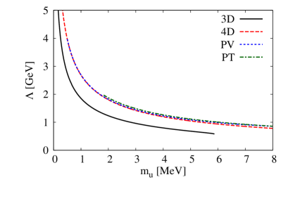
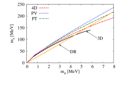
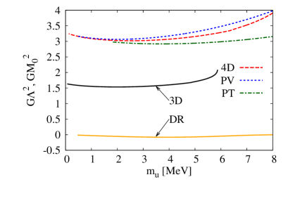
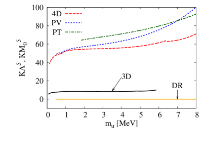


Figure 1 shows the resulting parameters with respect to . One observes that monotonically decreases with increasing , while increases according to , from upper left and right panels. There are no set of solutions under the conditions discussed in Sec. 3.1 in the 3D, 4D, PT and DR for large (small) region. Note that there are two sets of solutions in the DR case, and we draw the curves for the higher dimension case here.
Middle two panels display the results of the coupling strengths, and , in which we note that these quantities stay almost constant for each regularization in MeV, and the curves in the 4D, PV and PT are rather close comparing to the other methods in this region. The DR case shows peculiar feature; is negative for all and is considerably smaller than the other four regularizations. We can say these are characteristic aspects within the DR case. The DR has two parameters on behalf of the cutoff scale, and , where we observe increases and the mass scale parameter decreases with respect to , respectively. We will present more detailed discussions on the behaviors of the obtained parameters in the next subsection with choosing the cutoff scale as the horizontal axis .
3.3 Fitted parameters with respect to
It is physically more appealing that we redisplay the parameters as the function of the model scale, , with obtained parameters, since one can observe how the physical quantities effectively flow according to the model scale in the current effective field theory.
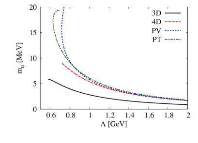
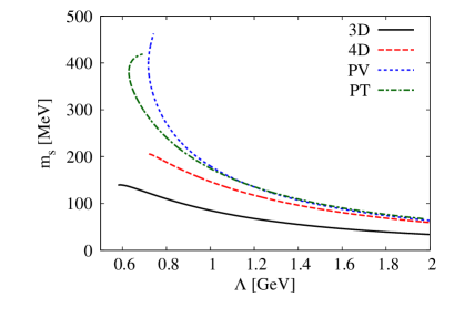
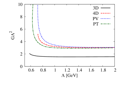
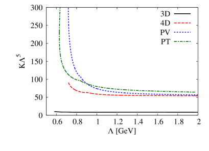
Figure 2 draws four parameters as the functions of the cutoff scale in the 3D, 4D, PV and PT. One sees that and decrease when becomes larger, while two couplings and decrease for small then approach almost constant for large . The PV and PT cases show the multi-valued functions for small cutoff scale, which is the characteristic feature seen in the PT case being also observed in the preceding analyses [27]. Qualitatively, we can say that all the regularization procedures show similar curves where each parameter becomes smaller when one takes larger cutoff scale. On the other hand quantitatively, the three regularizations, 4D, PV and PT lead close curves, whose values are much larger than the case in the 3D. This can easily be understood, because the 4D, PV and PT methods have the mathematically similar structure, while the 3D cutoff separately perform the time and space integrals.


We align the resulting parameters for the DR case in Fig. 3 where we chose the horizontal axis to be as mentioned above. It should be noted that the DR has two sets of solutions under the conditions discussed above. As is seen in the figure, we indicate the solutions with higher and the lower dimensions by denoting and , respectively. One sees that the current quark masses, and , decrease according to in the DR method, whose tendencies and the values are similar to the cases with the other regularizations. Note that the increase of means the decrease of as seen in Fig. 1. While the couplings and show non-monotonic curves for the higher dimensional case, , which is distinguishing feature of the . We will consider the cause on this non-monotonic behavior of the couplings in Sec. 5. It is noted that for each parameter, the existing region of the case is considerably narrow compare to the .
It is also interesting to mention that the parameters exist for considerably higher scale up to several GeV; where we do not show upper limit since the models are no longer reliable for such high scale. While the lower limits are important because they are comparable to hadronic scale and it has a strong regularization dependence. Here we numerically find the following values for lower limits:
| (55) |
On the other hand, there does not appear the lower limit in the DR case; the curves can be drawn in the limit. It may also be interesting to note that we have the upper limit in the DR. As is seen in the lower panel of Fig. 3, the value is around GeV. This limit stems from the restriction on the dimension, .
3.4 Table of Parameters
We have drawn the tendency of the parameters according to in Sec. 3.3. We now align the values of parameters in the table form. It will be useful for the study of the meson properties and the various physical phenomena such as chiral phase transition based on the NJL model. We also align the parameter sets obtained in the preceding analyses for various regularization methods, then make the numerical comparison among them.
| (MeV) | (MeV) | (MeV) | (MeV) | (MeV) | Ref. | ||
| 960.4 | 3.00 | 89.45 | 1.552 | 8.339 | 212 | 417 | |
| 681.6 | 5.00 | 128.3 | 1.706 | 8.772 | 286 | 487 | |
| 630.9 | 5.50 | 135.9 | 1.814 | 9.165 | 324 | 519 | |
| 625.4 | 5.55 | 136.6 | 1.830 | 9.246 | 330 | 524 | |
| 580.5 | 5.87 | 139.1 | 2.087 | 10.08 | 414 | 592 | |
| 335 | 527 | [6] | |||||
| 367.7 | 549.5 | [7] |
| (MeV) | (MeV) | (MeV) | (MeV) | (MeV) | Ref. | ||
| 1421 | 3.00 | 94.41 | 3.026 | 55.02 | 191 | 400 | |
| 1046 | 5.00 | 139.1 | 3.156 | 57.80 | 228 | 445 | |
| 850.2 | 7.00 | 176.5 | 3.526 | 64.30 | 280 | 499 | |
| 772.4 | 8.14 | 194.8 | 3.990 | 72.60 | 330 | 545 | |
| 719.3 | 8.99 | 205.5 | 5.341 | 91.99 | 453 | 648 | |
| 1049 | 5.0 | – | 3.741 | – | 222.3 | – | [15] (2f.) |
| 854 | 7.0 | – | 4.230 | – | 270.9 | – | [15] (2f.) |
| (MeV) | (MeV) | (MeV) | (MeV) | (MeV) | Ref. | ||
| 1443 | 3.00 | 102.7 | 3.094 | 59.83 | 188 | 385 | |
| 1085 | 5.00 | 158.0 | 3.305 | 68.29 | 218 | 420 | |
| 910.9 | 7.00 | 210.5 | 3.705 | 85.61 | 248 | 454 | |
| 743.3 | 11.8 | 327.8 | 5.885 | 175.5 | 330 | 534 | |
| 717.7 | 15.6 | 396.6 | 9.282 | 310.3 | 404 | 585 | |
| 214 | 397 | [20] | |||||
| 286 | 485 | [20] |
| (MeV) | (MeV) | (MeV) | (MeV) | (MeV) | Ref. | ||
| 1489 | 3.00 | 100.2 | 2.926 | 68.03 | 172 | 383 | |
| 1115 | 5.00 | 150.4 | 2.941 | 74.97 | 194 | 418 | |
| 924.1 | 7.00 | 195.6 | 3.059 | 85.50 | 216 | 451 | |
| 650.9 | 14.5 | 338.6 | 5.169 | 159.9 | 330 | 593 | |
| 629.0 | 17.2 | 380.9 | 7.493 | 222.4 | 415 | 665 | |
| 1080 | 5.0 | – | 3.802 | – | 216 | – | [29](2f.) |
| 907 | 7.0 | – | 4.138 | – | 240 | – | [29](2f.) |
| (MeV) | (MeV) | (MeV) | (MeV) | (MeV) | Ref. | |||
| 1353 | 2.368 | 3.00 | 79.23 | 0.06658 | ||||
| 1170 | 2.515 | 4.00 | 106.6 | 0.1604 | ||||
| 935.5 | 2.677 | 5.00 | 134.3 | 0.2371 | ||||
| 667.8 | 2.853 | 6.00 | 162.3 | 0.1814 | ||||
| 380.1 | 3.044 | 7.00 | 190.6 | 0.04530 | ||||
| – | – | – | [10] (2f.) | |||||
| – | – | – | [10] (2f.) |
| (MeV) | (MeV) | (MeV) | (MeV) | (MeV) | Ref. | |||
| 1489 | 2.289 | 3.00 | 85.26 | 0.09688 | ||||
| 1421 | 2.379 | 4.00 | 118.6 | 0.3459 | ||||
| 1351 | 2.463 | 4.94 | 157.1 | 1.433 | ||||
| – | – | – | [10] (2f.) | |||||
| – | – | – | [10] (2f.) |
In Tab. 1, our result is almost coincident with the one in Ref. [6]. The slight difference comes from the input parameter. The difference of between our result and Ref. [7] is caused by the definition of the mass, the former only considers the real part of the propagator, while the latter includes the imaginary part. In the 4D and PT cases, our results are close to the previous ones which obtained by two-flavor NJL model. Ref. [15] uses the decay width of as the input parameter. In Tab. 3, our result is close to the previous one [20] except for the value of . To obtain the meson mass spectra, the generalized heat kernel expansion are used in Ref. [20]. Although there exists one set of solution in the two-flavor model, two sets of solutions appear in the three-flavor case. As decreasing the cutoff scale , and increase in the and decrease in the .
4 Model predictions
The model parameters have been carefully fitted in the previous section. We are now ready for investigating various predicted quantities; in this section we are going to analyze the chiral condensates and constituent quark masses, the meson properties and the topological susceptibility. As is well known, the model predictions depend on the regularization methods and the model parameters, whose test is the focus we will study here.
4.1 Chiral condensates and constituent quark masses
The chiral condensates are the key quantities in this kind of model, since they are intimately related to the chiral symmetry breaking of the system and critically determine the model behavior. The constituent quark masses are also important physical objects which explicitly appear in the equations for the meson properties as shown in the Appendix. Since the mass of the proton and neutron are around GeV, then we naively expect that the values of the constituent masses for up and down quarks are around GeV, i.e., MeV. We will confirm that this value is consistently achieved within reliable model scale in the current models.
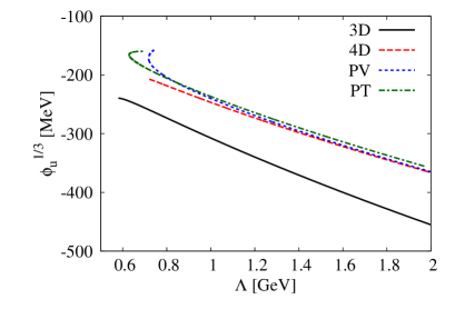
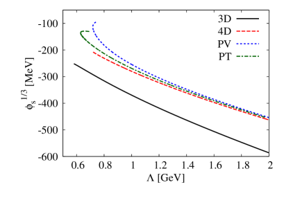
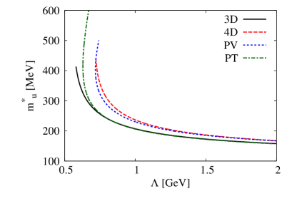
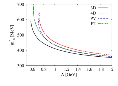
Figure 4 displays the results of the chiral condensates and the constituent quark masses with the fitted parameters shown in the previous subsection. One notes that the absolute values of monotonically increase with the cutoff, while decrease with respect to . Observing the obtained values, we see that the regions for GeV have nice numerical plots, MeV and MeV. One also notes that the constituent quark masses become nearly constant for high cutoff scale in all regularization cases. This characteristic may show us some universal properties that the constituent quark masses possess, which we will discuss in more detail in Sec. 5.1.


We exhibit the resulting chiral condensates and constituent masses in the DR method in Fig. 5. The qualitative tendency of the chiral condensates are similar to the other regularization ways as compared with the upper two panels of Fig. 4 where the absolute values of become larger with increasing the model scale. On the other hand, for the constituent quark masses, one notices the crucial difference between the DR and the other prescriptions; the signs of the constituent quark masses are opposite. This comes from the mathematical treatment of the analytic continuation when we regularize the loop integrals. The sign of the constituent quark masses can be positive with the counter terms [34]. The absolute values of the constituent quark masses decrease according to the model scale, which is the case for all the regularizations.
4.2 Meson properties and topological susceptibility
In this subsection we calculate the predicted meson properties, the meson mass , the kaon decay constant , the sigma meson mass and the topological susceptibility through using the fixed parameters. It is practically interesting, since the numerics are effectively important in determining whether the model and the employed methods including the choice of parameters are appropriate, eventually to be tested by experiments.
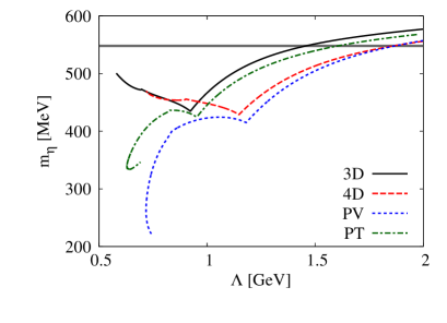
Figure 6 displays the obtained results for the mass in each regularization. Since the mass is one of the input quantities used for the fitting in the DR, it is fixed at GeV. We see that the obtained values are smaller than the experimental data for being the hadronic scale, while the experimental line crosses for relatively larger . The curves for the 3D and 4D indicate similar structures; they decrease upto some , then turn to increase for large scale. The curves in the PV and PT cases show almost monotonic behavior; they become larger with increasing . In any regularization, there appears typical cusp around GeV, which comes from the complex property due to the determinantal form of the equation (82) for and masses.
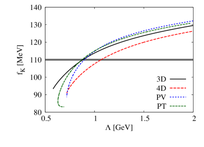

The kaon decay constants are shown in Fig. 7, where the results for the 3D, 4D, PV and PT all increase with the cutoff scale (left panel), while it becomes smaller according to in the DR. In GeV the curves for the 3D, PV and PT have similar behavior, while the curve for 4D shows a smaller than the others. It is interesting that the results for 3D, PT and PT have close value to the experimental data at almost same cutoff scale, GeV.
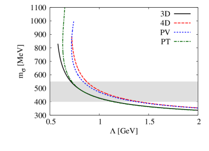

The sigma meson mass, , is evaluated as a pole of the propagator calculated from the loop integral of the scalar channel calculated by Eq. (69), whose results are exhibited in Fig. 8. The numbers obtained in the four regularizations observed in the left panel have reliable range compare to the empirical value, MeV [37], while the DR curves read the considerably larger values than the empirical scale. In the DR the pole of the sigma meson propagator does not exist for GeV, we regard the maximum value as the sigma meson mass in such region [31]. Contrary to the case for the mass, the mass decreases monotonically with respect to the model scale, which stems from the monotonic function of the equation for the sigma meson.
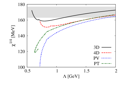

Finally in Fig. 9, we show the topological susceptibility calculated through the topological charge density presented in A.4. We note that the result in the 3D case is the closest to the one by the lattice QCD simulations, and the curves in the 4D, PV and PT enter the consistent region with lattice QCD for high , while the DR does not touch the gray region. It is interesting to see that the obtained curves show a certain similarity with the results of mass; the 3D and 4D plots decrease for small then increase for large while the PV and PT cases go up with increasing . The reason may be originated from the resembling systems of the equations for and where the matrix form, in particular the nonzero off diagonal elements due to the anomaly, plays a crucial role. The results in the DR are almost constant around MeV which is larger than the other regularization methods. Since one extra parameter is introduced in DR, the meson mass is fixed as an input parameter. If we accept some tolerance for the meson mass which is used as an input parameter, we can find a smaller topological susceptibility [32].
5 Discussions
The paper has been devoted to the systematic analyses on the parameter fitting and resulting predictions within various regularization procedures. We think now it may be intriguing that we give the detailed speculation on the tendency of the obtained parameters and the model predictions.
5.1 High scale behavior
Although the model is no longer effective for very high energy scale above GeV, we think that it is still worth studying how the model behaves at high energy. Here we are going to present the analysis on the asymptotic behavior of the current model. From the resulting parameters evaluated in Fig. 2, we note the interesting feature that the dimensionless coupling strengths and seem to approach some constant values at large limit. This can be understood by the discussions along Ref. [35]. For example, in the 3D case we read the dominant contribution of ,
| (56) |
in the gap equation (3). Then we have
| (57) |
From Figs. 2 and 4, the relations, , , and , can be read for high , then we see
| (58) |
In the same way, we have
| (59) |
in the 4D case. By noting that the PV and PT cases have the same asymptotic behavior with the 4D methods, then we expect that the approaches to in the 3D case, and in the 4D, PV, and PT methods. Our numerical results are for GeV in the 3D, for GeV in the 4D, for GeV and for GeV in the PT. These results seem to support the above discussion. By following the similar analyses on the equation for the masses, we can also confirm the asymptotic behavior of . This is the numerical reason why the two coupling strengths approach to some constant values at high energy limit.
5.2 Remarks on the dimensional regularization
We have used the quantity as the counterpart of the cutoff scale in the DR with fixed . It may be worth reconsidering on whether the current treatment is appropriate for the model analyses here. Since the DR makes integrals finite by changing the integral kernel, not by restricting the integration interval, the relation between these two scales are actually not quite clear in this effective model approach. The typical integrals go to infinity in the limit, so one might think it is nice to treat limit as the counterpart of the limit. However, the integral in the limit can be finite thanks to the conditions in subsection 3.1. The key point is the relationship between the mass scale parameter, , and which works so as to suppress the integral for higher dimensions ( for ) as studied in [35, 36]. Due to this suppression, the resulting integrals, meaning the integrals with factor , do not necessarily increase with respect to . Other correspondences between the cutoff and the dimensional regularizations are discussed in Refs. [15] and [30]. Based on the above discussion and the observation of the tendencies on the obtained model parameters and the predicted quantities, we think that our present treatment is effectively acceptable and the mass scale parameter can be considered as the quantity which closely relates to a cutoff scale.
5.3 System of parameter fitting
As the final discussion on the parameter fitting, we present the fact that the fitting, in particular, the existence of the parameters is sensitively determined by the property of the mass equation.
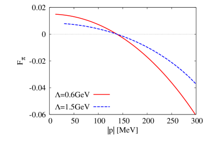
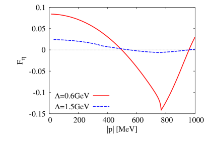
Figure 10 displays the typical results on the functions for the pion and masses; where the intersection points between each curve and dashed line indicate the values of the meson masses, MeV) and MeV). Since the qualitative feature of the functions is similar in the other regularization cases, we show the results of the 3D cutoff method as the representative figure for the explanation on the parameter fitting. It is also worth mentioning that the curve for the kaon equation is similar to the pion case. One notes that the equations for the pion present monotonic decrease with respect to , while the result for the mass function exhibits some complex structure. This comes from the determinantal form of the equation, which is due to the non-vanishing off-diagonal elements in the system as explicitly seen in the Appendix A.3.
The properties with changing on the functions are as follows. Although the slope with respect to , namely , changes according to for , we can always find the solution. On the other hand, the change of the slope of becomes important when we try to find the solutions on it; the absolute value of the slope decreases with increasing as seen from Fig. 10, then the range of gets smaller for high , leading the numerical difficulty of searching the solution. For small , on the other hand, the absolute value of the slope becomes larger, which leads the move of the curve and we eventually reach the point where we can no longer find the solution for MeV at some low . Thus the parameter fitting is sensitively affected by the equation for determining the mass.
6 Summary and conclusions
In this paper we have applied various regularization procedures to the NJL model then carried out the meticulous parameter fitting. One of the main results of this paper is the parameters sets investigated in the same conditions and the input quantities for each regularization. Similar behavior is observed for the model parameters in the 4D, PV and PT. The model parameters are determined even for extremely high scale beyond the hadronic energy, which, we think, is surely interesting since one can consider the ultraviolet region of the model. So we analyzed the asymptotic behavior of the model through considering the limit. We then analyzed the asymptotic behavior of the model through considering the limit. Where we saw the coupling strengths in the dimensionless form, and , for the effective four- and six-point interactions approach to constant values. This is as well the interesting feature of the current model.
After setting the model parameters, we evaluated the predicted values, and in each regularization. We studied whether the predicted quantities can indicate the values close to the experimental observations. We found that the obtained physical predictions show satisfactory close values to the empirical ones in the 3D, 4D, PV and PT methods, while some quantity has different order in the DR. This may indicate that the higher order corrections may be important due to the change of an integral kernel with smaller spacetime dimensions in the dimensional regularization. It should be noticed that one extra parameter is necessary in DR case. Thus we impose to generate the meson mass as input. If we relax the condition, we can find a parameters set to show more appropriate value for the other physical predictions.
We believe that the current analyses is useful for the readers who want to investigate the properties of mesons and hadrons, the transition phenomena of QCD such as the chiral phase transition, and the calculation procedures in various regularizations. Also, we think the obtained model parameters are useful since they enable us to study a lot of physical quantities by using various regularization methods. We plan to study the phase transition of the chiral symmetry breaking by using the obtained parameters in various regularization methods in future.
Acknowledgements
HK is supported by MOST 103-2811-M-002-087. TI is supported by JSPS KAKENHI Grant Number 26400250 and and 15H03663.
Appendix A Meson properties and topological susceptibility
Here we present the prescriptions on how one studies the physical observables in the current model treatment. The masses of mesons are investigated by using the Bethe-Salpeter equations which give the green functions for the composite particles. Similarly, the decay constants for mesons and the topological susceptibility are evaluated based on the diagrammatic calculations incorporating the constituent quark propagator. The detailed derivations of the equations are presented in some review papers, see for instance [5].
A.1 Pion, sigma and kaon masses
The masses of the pion, sigma and kaon are evaluated at the pole position of the propagators derived from the random phase approximation with the leading order of the expansion. The propagators for these mesons are given by
| (60) |
with the effective couplings for each channel ( and ),
| (61) | |||||
| (62) |
and the quark-antiquark loop contributions are given by
| (63) | |||
| (64) | |||
| (65) |
for each meson with
| (66) | |||||
| (67) |
where the suffices and indicate the pseudo-scalar and scalar channels, respectively. One obtains the following expressions after a bit of algebra
| (68) | |||||
| (69) |
Since the following relations should hold
| (70) |
at the pole position, then the meson mass is given by Eq. (70).
A.2 Pion and kaon decay constants
The pion and kaon decay constant are calculated through evaluating the following one-loop amplitude,
| (71) |
with for channels and for channels, and the coupling strengths for the meson-quark-quark interaction, , evaluated by
| (72) |
After some algebra, we have
| (73) | |||||
| (74) |
where equations are evaluated at and give the pion and kaon decay constants, respectively [5].
A.3 and masses
Compared with the pion and kaon masses, there appears the complexity for the – system, where the propagator can be written by the matrix form as
| (75) |
where and represent matrices whose elements are given by
| (76) | |||||
| (77) | |||||
| (78) | |||||
| (79) | |||||
| (80) | |||||
| (81) |
Then the condition which determines the and masses becomes
| (82) |
The explicit expressions for the numerical calculations are shown in [32].
A.4 Topological susceptibility
References
- [1] Y. Nambu and G. Jona-Lasinio, Phys. Rev. 122, 345 (1961); Y. Nambu and G. Jona-Lasinio, 124 (1961) 246.
- [2] S. Weinberg, Phys. Rev. D 11 (1975) 3583.
- [3] M. Kobayashi and T. Maskawa, Prog. Theor. Phys. 44 (1970) 1422; M. Kobayashi, H. Kondo and T. Maskawa, Prog. Theor. Phys. 45 (1971) 1955; G. ’t Hooft, Phys. Rev. D 14 (1976) 3432; G. ’t Hooft, Phys. Rev. D 18 (1978) 2199 (Erratum); G. ’t Hooft, Phys. Rept. 142 (1986) 357.
- [4] U. Vogl and W. Weise, Prog. Part. Nucl. Phys. 27 (1991) 195.
- [5] S. P. Klevansky, Rev. Mod. Phys. 64 (1992) 649.
- [6] T. Hatsuda and T. Kunihiro, Phys. Rept. 247 (1994) 221.
- [7] P. Rehberg, S. P. Klevansky and J. Hufner, Phys. Rev. C 53 (1996) 410.
- [8] M. Buballa, Phys. Rept. 407 (2005) 205.
- [9] M. Huang, Int. J. Mod. Phys. E 14 (2005) 675.
- [10] H. Kohyama, D. Kimura and T. Inagaki, Nucl. Phys. B 896 (2015) 682.
- [11] W. Pauli and F. Villars, Rev. Mod. Phys. 21 (1949) 434.
- [12] C. Itzykson and J. B. Zuber, Quantum Field Theory (McGrow-Hill Inc. Press, 1980).
- [13] T. P. Cheng and L. F. Li, Gauge Theory of Elementary Particle Physics (Oxford University Press, 1984).
- [14] J. S. Schwinger, Phys. Rev. 82 (1951) 664.
- [15] S. Krewald and K. Nakayama, Annals Phys. 216 (1992) 201.
- [16] R. G. Jafarov and V. E. Rochev, Central Eur. J. Phys. 2 (2004) 367.
- [17] R. G. Jafarov, and V. E. Rochev, Russ. Phys. J. 49 (2006) 364; R. G. Jafarov, and V. E. Rochev, Izv. Vuz. Fiz. 49 (2006) 20.
- [18] M. Jaminon, P. Stassart and G. Ripka, Phys. Lett. B 227 (1989) 191.
- [19] D. Kahana and M. Lavelle, Phys. Lett. B 298 (1993) 397.
- [20] A. A. Osipov, H. Hansen and B. Hiller, Nucl. Phys. A 745 (2004) 81.
- [21] J. Moreira, B. Hiller, A. A. Osipov and A. H. Blin, Int. J. Mod. Phys. A 27 (2012) 1250060.
- [22] H. Suganuma and T. Tatsumi, Annals Phys. 208 (1991) 470.
- [23] K. G. Klimenko, Z. Phys. C 54 (1992) 323.
- [24] V. P. Gusynin, V. A. Miransky and I. A. Shovkovy, Phys. Rev. Lett. 73 (1994) 3499; V. P. Gusynin, V. A. Miransky and I. A. Shovkovy, Phys. Rev. Lett. 76 (1996) 1005 (Erratum).
- [25] T. Inagaki, S. D. Odintsov and Y. I. Shil’nov, Int. J. Mod. Phys. A 14 (1999) 481.
- [26] T. Inagaki, D. Kimura and T. Murata, Prog. Theor. Phys. Suppl. 153 (2004) 321.
- [27] T. Inagaki, D. Kimura and T. Murata, Prog. Theor. Phys. 111 (2004) 371.
- [28] T. Inagaki, D. Kimura and T. Murata, Int. J. Mod. Phys. A 20 (2005) 4995.
- [29] Z. F. Cui, Y. L. Du and H. S. Zong, Int. J. Mod. Phys. Conf. Ser. 29 (2014) 1460232.
- [30] T. Inagaki, T. Muta and S. D. Odintsov, Prog. Theor. Phys. Suppl. 127 (1997) 93.
- [31] T. Inagaki, D. Kimura and A. Kvinikhidze, Phys. Rev. D 77 (2008) 116004.
- [32] T. Inagaki, D. Kimura, H. Kohyama and A. Kvinikhidze, Phys. Rev. D 83 (2011) 034005.
- [33] T. Inagaki, D. Kimura, H. Kohyama and A. Kvinikhidze, Phys. Rev. D 85 (2012) 076002.
- [34] T. Inagaki, D. Kimura, H. Kohyama and A. Kvinikhidze, Phys. Rev. D 86 (2012) 116013.
- [35] T. Inagaki, D. Kimura, H. Kohyama and A. Kvinikhidze, Int. J. Mod. Phys. A 28 (2013) 1350164.
- [36] T. Inagaki, D. Kimura and H. Kohyama, Int. J. Mod. Phys. A 29 (2014) 1450048.
- [37] K. A. Olive et al. [Particle Data Group Collaboration], Chin. Phys. C 38 (2014) 090001.
- [38] B. Alles, M. D’Elia and A. Di Giacomo, Nucl. Phys. B 494 (1997) 281; B. Alles, M. D’Elia and A. Di Giacomo, Nucl. Phys. B 679 (2004) 397 (Erratum).
- [39] K. Fukushima, K. Ohnishi and K. Ohta, Phys. Rev. C 63 (2001) 045203.