Small sample methods for cluster-robust variance estimation and hypothesis testing in fixed effects models

Abstract

In panel data models and other regressions with unobserved effects, fixed effects estimation is often paired with cluster-robust variance estimation (CRVE) in order to account for heteroskedasticity and un-modeled dependence among the errors. Although asymptotically consistent, CRVE can be biased downward when the number of clusters is small, leading to hypothesis tests with rejection rates that are too high. More accurate tests can be constructed using bias-reduced linearization (BRL), which corrects the CRVE based on a working model, in conjunction with a Satterthwaite approximation for t-tests. We propose a generalization of BRL that can be applied in models with arbitrary sets of fixed effects, where the original BRL method is undefined, and describe how to apply the method when the regression is estimated after absorbing the fixed effects. We also propose a small-sample test for multiple-parameter hypotheses, which generalizes the Satterthwaite approximation for t-tests. In simulations covering a wide range of scenarios, we find that the conventional cluster-robust Wald test can severely over-reject while the proposed small-sample test maintains Type I error close to nominal levels. The proposed methods are implemented in an R package called clubSandwich.

This paper has been revised to correct an error in the statement of Theorem 2 and minor typos in the proof of Theorem 1.

Keywords: cluster dependence, fixed effects, robust standard errors, small samples

1 INTRODUCTION

In many economic analyses, interest centers on the parameters of a linear regression model estimated by ordinary or weighted least squares from data exhibiting within-group dependence. Such dependence can arise from sampling or random assignment of aggregate units (e.g., counties, districts, villages), each of which contains multiple observations; from repeated measurement of an outcome on a common set of units, as in panel data; or from model misspecification, as in analysis of regression discontinuity designs (e.g., Lee and Card 2008). A common approach to inference in these settings is to use a cluster-robust variance estimator (CRVE, Arellano 1987; Liang and Zeger 1986; White 1984). The advantage of the CRVE is that it produces consistent standard errors and test statistics without imposing strong parametric assumptions about the correlation structure of the errors in the model. Instead, the method relies on the weaker assumption that units can be grouped into clusters that are mutually independent. In the past decade, use of CRVEs has become standard practice for micro-economic researchers, as evidenced by coverage in major textbooks and review articles (e.g., Wooldridge 2010; Angrist and Pischke 2009; Cameron and Miller 2015).

As a leading example, consider a difference-in-differences analysis of state-by-year panel data, where the goal is to understand the effects on employment outcomes of several state-level policy shifts. Each policy effect would be parameterized as a dummy variable in a regression model, which might also include other demographic controls. It is also common to include fixed effects for states and time-points in order to control for unobserved confounding in each dimension. The model could be estimated by least squares with the fixed effects included as dummy variables (or what we will call the LSDV estimator). More commonly, the effects of the policy indicators would be estimated after absorbing the fixed effects, a computational technique that is also known as the fixed effects estimator or “within transformation” (Wooldridge 2010). Standard errors would then be clustered by state to account for residual dependence in the errors from a given state, and these clustered standard errors would be used to test hypotheses about the set of policies. The need to cluster the standard errors by state, even when including state fixed effects, was highlighted by Bertrand, Duflo, and Mullainathan (2004), who showed that to do otherwise can lead to inappropriately small standard errors and hypothesis tests with incorrect rejection rates.

The consistency property of CRVEs is asymptotic in the number of independent clusters (Wooldridge 2003). Recent methodological work has demonstrated that CRVEs can be biased downward and associated hypothesis tests can have Type-I error rates considerably in excess of nominal levels when based on a small or moderate number of clusters (e.g., MacKinnon and Webb 2016). Cameron and Miller (2015) provided an extensive review of this literature, including a discussion of current practice, possible solutions, and open problems. In particular, they demonstrated that small-sample corrections for t-tests implemented in common software packages such as Stata and SAS do not provide adequate control of Type-I error.

Bell and McCaffrey (2002) proposed a method that improves the small-sample properties of CRVEs (see also McCaffrey, Bell, and Botts 2001). The method, called bias-reduced linearization (BRL), entails adjusting the CRVE so that it is exactly unbiased under a working model specified by the analyst, while also remaining asymptotically consistent under arbitrary true variance structures. Simulations reported by Bell and McCaffrey (2002) demonstrate that the BRL correction serves to reduce the bias of the CRVE even when the working model is misspecified. The same authors also proposed small-sample corrections to single-parameter hypothesis tests using the BRL variance estimator, based on Satterthwaite (Bell and McCaffrey 2002) or saddlepoint approximations (McCaffrey and Bell 2006). In an analysis of a longitudinal cluster-randomized trial with 35 clusters, Angrist and Lavy (2009) observed that the BRL correction makes a difference for inferences.

Despite a growing body of evidence that BRL performs well (e.g., Imbens and Kolesar 2016), several problems with the method hinder its wider application. First, Angrist and Pischke (2009) noted that the BRL correction is undefined in some commonly used models, such as state-by-year panels that include fixed effects for states and for years (see also Young 2016). Second, in models with fixed effects, the magnitude of the BRL adjustment depends on whether it is computed based on the full design matrix (i.e., the LSDV estimator) or after absorbing the fixed effects. Third, extant methods for hypothesis testing based on BRL are limited to single-parameter constraints (Bell and McCaffrey 2002; McCaffrey and Bell 2006) and small-sample methods for multiple-parameter hypothesis tests remain lacking.

This paper addresses each of these concerns in turn, with the aim of extending the BRL method so that is suitable for general application. First, we describe a simple modification of the BRL adjustment that remains well-defined in models with arbitrary sets of fixed effects, where existing BRL adjustments break down. Second, we demonstrate how to calculate the BRL adjustments based on the fixed effects estimator and identify conditions under which first-stage absorption of the fixed effects can be ignored. Finally, we propose a procedure for testing multiple-parameter hypotheses by approximating the sampling distribution of the Wald statistic using Hotelling’s $T^{2}$ distribution with estimated degrees of freedom. The method is a generalization of the Satterthwaite correction proposed by Bell and McCaffrey (2002) for single parameter constraints. The proposed methods are implemented in the R package clubSandwich, which is available on the Comprehensive R Archive Network.

Our work is related to a stream of recent literature that has examined methods for cluster-robust inference with a small number of clusters. Conley and Taber (2011) proposed methods for hypothesis testing in a difference-in-differences setting where the number of treated units is small and fixed, while the number of untreated units increases asymptotically. Ibragimov and Müller (2010, 2016) proposed cluster-robust t-tests that maintain the nominal Type-I error rate by re-weighting within-cluster estimators of the target parameter. Young (2016) proposed a Satterthwaite correction for t-tests based on a different type of bias correction to the CRVE, where the bias correction term is derived under a working model. Cameron, Gelbach, and Miller (2008) investigated a range of bootstrapping procedures that provide improved Type-I error control in small samples, finding that a cluster wild-bootstrap technique was particularly accurate in small samples. Nearly all of this work has focused on single-parameter hypothesis tests only. For multiple-parameter constraints, Cameron and Miller (2015) suggested an ad hoc degrees of freedom adjustment and noted, as an alternative, that bootstrapping techniques can in principle be applied to multiple-parameter tests. However, little methodological work has examined the accuracy of multiple-parameter tests.

The paper is organized as follows. The remainder of this section introduces our econometric framework and reviews standard CRVE methods, as implemented in most software applications. Section 2 reviews the original BRL correction and describes modifications that make it possible to implement BRL in a broad class of models with fixed effects. Section 3 discusses hypothesis tests based on the BRL-adjusted CRVE. Section 4 reports a simulation study examining the null rejection rates of multiple-parameter hypothesis tests, where we find that the small-sample test offers drastic improvements over commonly implemented alternatives. Section 5 illustrates the use of the proposed hypothesis tests in two applications. Section 6 concludes and discusses avenues for future work.

1.1 Econometric framework

We consider a linear regression model of the form,

$$\mathbf{y}_{i}=\mathbf{R}_{i}\boldsymbol{\beta}+\mathbf{S}_{i}\boldsymbol{\gamma}+\mathbf{T}_{i}\boldsymbol{\mu}+\boldsymbol{\epsilon}_{i},$$ (1)

where there are a total of $m$ clusters; cluster $i$ contains $n_{i}$ units; $\mathbf{y}_{i}$ is a vector of the $n_{i}$ values of the outcome for units in cluster $i$; $\mathbf{R}_{i}$ is an $n_{i}\times r$ matrix containing predictors of primary interest (e.g., policy variables) and any additional controls; $\mathbf{S}_{i}$ is an $n_{i}\times s$ matrix describing fixed effects that are identified across multiple clusters; and $\mathbf{T}_{i}$ is an $n_{i}\times t$ matrix describing cluster-specific fixed effects, which must satisfy $\mathbf{T}_{h}\mathbf{T}_{i}^{\prime}=\mathbf{0}$ for $h\neq i$. Note that the distinction between the covariates $\mathbf{R}_{i}$ versus the fixed effects $\mathbf{S}_{i}$ is arbitrary and depends on the analyst’s inferential goals. In a fixed effects model for state-by-year panel data, $\mathbf{R}_{i}$ would include variables describing policy changes, as well as additional demographic controls; $\mathbf{S}_{i}$ would include year fixed effects; and $\mathbf{T}_{i}$ would indicate state fixed effects (and perhaps also state-specific time trends). Interest would center on testing hypotheses regarding the coefficients in $\boldsymbol{\beta}$ that correspond to the policy indicators, while $\boldsymbol{\gamma}$ and $\boldsymbol{\mu}$ would be treated as incidental.

We shall assume that $\text{E}\left(\boldsymbol{\epsilon}_{i}\left|\mathbf{R}_{i},\mathbf{S}_{i},\mathbf{T}_{i}\right.\right)=\mathbf{0}$ and $\text{Var}\left(\boldsymbol{\epsilon}_{i}\left|\mathbf{R}_{i},\mathbf{S}_{i},\mathbf{T}_{i}\right.\right)=\boldsymbol{\Sigma}_{i}$, for $i=1,...,m$, where the form of $\boldsymbol{\Sigma}_{1},...,\boldsymbol{\Sigma}_{m}$ may be unknown but the errors are independent across clusters. Let $\mathbf{U}_{i}=\left[\mathbf{R}_{i}\ \mathbf{S}_{i}\right]$ denote the set of predictors that are identified across multiple clusters, $\mathbf{X}_{i}=\left[\mathbf{R}_{i}\ \mathbf{S}_{i}\ \mathbf{T}_{i}\right]$ denote the full set of predictors, $\boldsymbol{\alpha}=\left(\boldsymbol{\beta}^{\prime},\boldsymbol{\gamma}^{\prime},\boldsymbol{\mu}^{\prime}\right)^{\prime}$, and $p=r+s+t$. Let $N=\sum_{i=1}^{m}n_{i}$ denote the total number of observations. Let $\mathbf{y}$, $\mathbf{R}$, $\mathbf{S}$, $\mathbf{T}$, $\mathbf{U}$, $\mathbf{X}$, and $\boldsymbol{\epsilon}$ denote the matrices obtained by stacking their corresponding components, as in $\mathbf{R}=\left(\mathbf{R}_{1}^{\prime}\ \mathbf{R}_{2}^{\prime}\ \cdots\ \mathbf{R}_{m}^{\prime}\right)^{\prime}$.

We assume that $\boldsymbol{\beta}$ is estimated by weighted least squares (WLS) using symmetric, full rank weighting matrices $\mathbf{W}_{1},...,\mathbf{W}_{m}$. Clearly, the WLS estimator includes ordinary least squares (OLS) as a special case. More generally, the WLS estimator encompasses feasible generalized least squares, where it is assumed that $\text{Var}\left(\mathbf{e}_{i}\left|\mathbf{X}_{i}\right.\right)=\boldsymbol{\Phi}_{i}$, a known function of a low-dimensional parameter. For example, an auto-regressive error structure might be posited to describe repeated measures on an individual over time. The weighting matrices are then taken to be $\mathbf{W}_{i}=\hat{\boldsymbol{\Phi}}_{i}^{-1}$, where the $\hat{\boldsymbol{\Phi}}_{i}$ are constructed from estimates of the variance parameter. Finally, for analysis of data from complex survey designs, WLS may be used with sampling weights in order to account for unequal selection probabilities.

1.2 Absorption

The goal of most analyses is to estimate and test hypotheses regarding the parameters in $\boldsymbol{\beta}$, while the fixed effects $\boldsymbol{\gamma}$ and $\boldsymbol{\mu}$ are not of inferential interest. Furthermore, LSDV estimation becomes computationally intensive and numerically inaccurate if the model includes a large number of fixed effects (i.e., $s+t$ large). A commonly implemented alternative to LSDV is to first absorb the fixed effects, which leaves only the $r$ parameters in $\boldsymbol{\beta}$ to be estimated. Because Section 2 examines the implications of absorption for application of the BRL adjustment, we now formalize this procedure. Denote the full block-diagonal weighting matrix as $\mathbf{W}=\text{diag}\left(\mathbf{W}_{1},...,\mathbf{W}_{m}\right)$. Let $\mathbf{K}$ be the $p\times r$ matrix that selects the covariates of interest, so that $\mathbf{X}\mathbf{K}=\mathbf{R}$ and $\mathbf{K}^{\prime}\boldsymbol{\alpha}=\boldsymbol{\beta}$. For a generic matrix $\mathbf{Z}$ of full column rank, let $\mathbf{M_{Z}}=\left(\mathbf{Z}^{\prime}\mathbf{W}\mathbf{Z}\right)^{-1}$ and $\mathbf{H_{Z}}=\mathbf{Z}\mathbf{M_{Z}}\mathbf{Z}^{\prime}\mathbf{W}$.

The absorption technique involves obtaining the residuals from the regression of $\mathbf{y}$ on $\mathbf{T}$ and from the multivariate regression of $[\mathbf{R}\ \mathbf{S}]$ on $\mathbf{T}$. The $\mathbf{y}$ residuals and $\mathbf{R}$ residuals are then regressed on the $\mathbf{S}$ residuals. Finally, these twice-regressed $\mathbf{y}$ residuals are regressed on the twice-regressed $\mathbf{R}$ residuals to obtain the WLS estimates of $\boldsymbol{\beta}$. Let $\mathbf{\ddot{S}}=\left(\mathbf{I}-\mathbf{H_{T}}\right)\mathbf{S}$, $\mathbf{\ddot{R}}=\left(\mathbf{I}-\mathbf{H_{\ddot{S}}}\right)\left(\mathbf{I}-\mathbf{H_{T}}\right)\mathbf{R}$, and $\mathbf{\ddot{y}}=\left(\mathbf{I}-\mathbf{H_{\ddot{S}}}\right)\left(\mathbf{I}-\mathbf{H_{T}}\right)\mathbf{y}$. In what follows, subscripts on $\mathbf{\ddot{R}}$, $\mathbf{\ddot{S}}$, $\mathbf{\ddot{U}}$, and $\mathbf{\ddot{y}}$ refer to the rows of these matrices corresponding to a specific cluster. The WLS estimator of $\boldsymbol{\beta}$ can then be written as

$$\boldsymbol{\hat{\beta}}=\mathbf{M_{\ddot{R}}}\sum_{i=1}^{m}\mathbf{\ddot{R}}_{i}^{\prime}\mathbf{W}_{i}\mathbf{\ddot{y}}_{i}.$$ (2)

This estimator is algebraically identical to the LSDV estimator, $\boldsymbol{\hat{\beta}}=\mathbf{K}^{\prime}\mathbf{M_{X}}\mathbf{X}^{\prime}\mathbf{W}\mathbf{y}$, but avoids the need to solve a system of $p$ linear equations. For further details on sequential absorption, see Davis (2002). In the remainder, we assume that fixed effects are absorbed before estimation of $\boldsymbol{\beta}$.

1.3 Standard CRVE

The WLS estimator $\boldsymbol{\hat{\beta}}$, has true variance

$$\text{Var}\left(\boldsymbol{\hat{\beta}}\right)=\mathbf{M_{\ddot{R}}}\left(\sum_{i=1}^{m}\mathbf{\ddot{R}}_{i}^{\prime}\mathbf{W}_{i}\boldsymbol{\Sigma}_{i}\mathbf{W}_{i}\mathbf{\ddot{R}}_{i}\right)\mathbf{M_{\ddot{R}}},$$ (3)

which depends upon the unknown variance matrices $\boldsymbol{\Sigma}_{i}$.

The CRVE involves estimating $\text{Var}\left(\boldsymbol{\hat{\beta}}\right)$ empirically, without imposing structural assumptions on $\boldsymbol{\Sigma}_{i}$. There are several versions of this approach, all of which can be written as

$$\mathbf{V}^{CR}=\mathbf{M_{\ddot{R}}}\left(\sum_{i=1}^{m}\mathbf{\ddot{R}}_{i}^{\prime}\mathbf{W}_{i}\mathbf{A}_{i}\mathbf{e}_{i}\mathbf{e}_{i}^{\prime}\mathbf{A}_{i}^{\prime}\mathbf{W}_{i}\mathbf{\ddot{R}}_{i}\right)\mathbf{M_{\ddot{R}}},$$ (4)

where $\mathbf{e}_{i}=\mathbf{Y}_{i}-\mathbf{X}_{i}\boldsymbol{\hat{\beta}}$ is the vector of residuals from cluster $i$ and $\mathbf{A}_{i}$ is some $n_{i}$ by $n_{i}$ adjustment matrix.

The form of the adjustment matrices parallels those of the heteroskedasticity-consistent variance estimators proposed by MacKinnon and White (1985). The original CRVE, described by Liang and Zeger (1986), uses $\mathbf{A}_{i}=\mathbf{I}_{i}$, an $n_{i}\times n_{i}$ identity matrix. Following Cameron and Miller (2015), we refer to this estimator as CR0. This estimator is biased towards zero because the cross-product of the residuals $\mathbf{e}_{i}\mathbf{e}_{i}^{\prime}$ tends to under-estimate the true variance $\boldsymbol{\Sigma}_{i}$ in cluster $i$. A rough bias adjustment is to take $\mathbf{A}_{i}=c\mathbf{I}_{i}$, where $c=\sqrt{(m/(m-1))}$; we denote this adjusted estimator as CR1. Some functions in Stata use a slightly different correction factor $c_{S}=\sqrt{(mN)/[(m-1)(N-p)]}$; we will refer to the adjusted estimator using $c_{S}$ as CR1S. When $N>>p$, $c_{S}\approx\sqrt{m/(m-1)}$ and so CR1 and CR1S will be very similar. However, CR1 and CR1S can differ quite substantially for models with a large number of fixed effects and small within-cluster sample size; recent guidance emphasizes that CR1S is not appropriate for this scenario (Cameron and Miller 2015). The CR1 and CR1S estimators are commonly used in empirical applications.

Use of these adjustments still tends to under-estimate the true variance of $\hat{\boldsymbol{\beta}}$ because the degree of bias depends not only on the number of clusters $m$, but also on skewness of the covariates and unbalance across clusters (Carter, Schnepel, and Steigerwald 2013; MacKinnon 2013; Cameron and Miller 2015; Young 2016). A more principled approach to bias correction would take into account the features of the covariates in $\mathbf{X}$. One such estimator uses adjustment matrices given by $\mathbf{A}_{i}=\left(\mathbf{I}-\mathbf{\ddot{R}}_{i}\mathbf{M_{\ddot{R}}}\mathbf{\ddot{R}}_{i}^{\prime}\mathbf{W}_{i}\right)^{-1}$. This estimator, denoted CR3, closely approximates the jackknife re-sampling estimator (Bell and McCaffrey 2002; Mancl and DeRouen 2001). However, CR3 tends to over-correct the bias of CR0, while the CR1 estimator tends to under-correct. The next section describes in detail the BRL approach, which makes adjustments that are intermediate in magnitude between CR1 and CR3.

2 BIAS REDUCED LINEARIZATION

The BRL correction is premised on a “working” model for the structure of the errors, which must be specified by the analyst. Under a given working model, adjustment matrices $\mathbf{A}_{i}$ are defined so that the variance estimator is exactly unbiased. We refer to this correction as CR2 because it extends the HC2 variance estimator for regressions with uncorrelated errors, which is exactly unbiased when the errors are homoskedastic (MacKinnon and White 1985). The idea of specifying a model may seem antithetical to the purpose of using CRVE, yet extensive simulation studies have demonstrated that the method performs well in small samples even when the working model is incorrect (Tipton 2015; Bell and McCaffrey 2002; Cameron and Miller 2015; Imbens and Kolesar 2016). Although the CR2 estimator might not be exactly unbiased when the working model is misspecified, its bias still tends to be greatly reduced compared to CR1 or CR0 (thus the name “bias reduced linearization”). Furthermore, as the number of clusters increases, reliance on the working model diminishes.

Let $\boldsymbol{\Phi}=\text{diag}\left(\boldsymbol{\Phi}_{1},...,\boldsymbol{\Phi}_{m}\right)$ denote a working model for the covariance structure (up to a scalar constant). For example, we might assume that the errors are uncorrelated and homoskedastic, with $\boldsymbol{\Phi}_{i}=\mathbf{I}_{i}$ for $i=1,...,m$. Alternatively, Imbens and Kolesar (2016) suggested using a random effects (i.e., compound symmetric) structure, in which $\boldsymbol{\Phi}_{i}$ has unit diagonal entries and off-diagonal entries of $\rho$, with $\rho$ estimated using the OLS residuals.

In the original formulation of Bell and McCaffrey (2002), the BRL adjustment matrices are chosen to satisfy the criterion

$$\mathbf{A}_{i}\left(\mathbf{I}-\mathbf{H_{X}}\right)_{i}\boldsymbol{\Phi}\left(\mathbf{I}-\mathbf{H_{X}}\right)_{i}^{\prime}\mathbf{A}_{i}^{\prime}=\boldsymbol{\Phi}_{i}$$ (5)

for a given working model, where $\left(\mathbf{I}-\mathbf{H_{X}}\right)_{i}$ denotes the rows of $\mathbf{I}-\mathbf{H_{X}}$ corresponding to cluster $i$. If the working model and weight matrices are both taken to be identity matrices, then the adjustment matrices simplify to $\mathbf{A}_{i}=\left(\mathbf{I}_{i}-\mathbf{X}_{i}\mathbf{M_{X}}\mathbf{X}_{i}^{\prime}\right)^{-1/2}$, where $\mathbf{Z}^{-1/2}$ denotes the symmetric square-root of the matrix $\mathbf{Z}$.

2.1 A more general BRL criterion

The original formulation of $\mathbf{A}_{i}$ is problematic because, for some fixed effects models that are common in economic applications, Equation 5 has no solution. Angrist and Pischke (2009) note that this problem occurs in balanced state-by-year panel models that include fixed effects for states and for years, where $\mathbf{I}_{i}-\mathbf{X}_{i}\mathbf{M_{X}}\mathbf{X}_{i}^{\prime}$ is not of full rank. Young (2016) reported that this problem occurred frequently when applying BRL to a large corpus of fitted regression models drawn from published studies.

This issue can be solved by using an alternative criterion to define the adjustment matrices, for which a solution always exists. Instead of (5), we propose to use adjustment matrices $\mathbf{A}_{i}$ that satisfy:

$$\mathbf{\ddot{R}}_{i}^{\prime}\mathbf{W}_{i}\mathbf{A}_{i}\left(\mathbf{I}-\mathbf{H_{X}}\right)_{i}\boldsymbol{\Phi}\left(\mathbf{I}-\mathbf{H_{X}}\right)_{i}^{\prime}\mathbf{A}_{i}^{\prime}\mathbf{W}_{i}\mathbf{\ddot{R}}_{i}=\mathbf{\ddot{R}}_{i}^{\prime}\mathbf{W}_{i}\boldsymbol{\Phi}_{i}\mathbf{W}_{i}\mathbf{\ddot{R}}_{i}.$$ (6)

A variance estimator that uses such adjustment matrices will be exactly unbiased when the working model is correctly specified.

A symmetric solution to Equation (6) is given by

$$\mathbf{A}_{i}=\mathbf{D}_{i}^{\prime}\mathbf{B}_{i}^{+1/2}\mathbf{D}_{i},$$ (7)

where $\mathbf{D}_{i}$ is the upper-right triangular Cholesky factorization of $\boldsymbol{\Phi}_{i}$,

$$\mathbf{B}_{i}=\mathbf{D}_{i}\left(\mathbf{I}-\mathbf{H_{X}}\right)_{i}\boldsymbol{\Phi}\left(\mathbf{I}-\mathbf{H_{X}}\right)_{i}^{\prime}\mathbf{D}_{i}^{\prime},$$ (8)

and $\mathbf{B}_{i}^{+1/2}$ is the symmetric square root of the Moore-Penrose inverse of $\mathbf{B}_{i}$. The Moore-Penrose inverse of $\mathbf{B}_{i}$ is well-defined and unique (Banerjee and Roy 2014, Thm. 9.18). In contrast, the original BRL adjustment matrices involve the symmetric square root of the regular inverse of $\mathbf{B}_{i}$, which does not exist when $\mathbf{B}_{i}$ is rank-deficient. If $\mathbf{B}_{i}$ is of full rank, then our adjustment matrices reduce to the original formulation described by Bell and McCaffrey (2002).

The adjustment matrices given by (7) and (8) satisfy criterion (6), as stated in the following theorem.

Theorem 1.

Let $\mathbf{L}_{i}=\left(\mathbf{\ddot{U}}^{\prime}\mathbf{W}\mathbf{\ddot{U}}-\mathbf{\ddot{U}}_{i}^{\prime}\mathbf{W}_{i}\mathbf{\ddot{U}}_{i}\right)$, where $\mathbf{\ddot{U}}=\left(\mathbf{I}-\mathbf{H_{T}}\right)\mathbf{U}$, and assume that $\mathbf{L}_{1},...,\mathbf{L}_{m}$ have full rank $r+s$. Further assume that $\text{Var}\left(\boldsymbol{\epsilon}_{i}\left|\mathbf{X}_{i}\right.\right)=\sigma^{2}\boldsymbol{\Phi}_{i}$, for $i=1,...,m$. Then the adjustment matrix $\mathbf{A}_{i}$ defined in (7) and (8) satisfies criterion (6) and the CR2 variance estimator is exactly unbiased.

Proof is given in Appendix A. The main implication of Theorem 1 is that, under our more general definition, the CR2 variance estimator remains well-defined even in models with large sets of fixed effects.

2.2 Absorption and LSDV Equivalence

In fixed effects regression models, a problem with the original definition of BRL is that it can result in a different estimator depending upon which design matrix is used. If $\boldsymbol{\beta}$ is estimated using LSDV, then it is natural to calculate the CR2 adjustment matrices based on the full covariate design matrix, $\mathbf{X}$. However, if $\boldsymbol{\beta}$ is estimated after absorbing the fixed effects, the analyst might choose to calculate the CR2 correction based on the absorbed covariate matrix $\mathbf{\ddot{R}}$—that is, by substituting $\mathbf{H_{\ddot{R}}}$ for $\mathbf{H_{X}}$ in (8)—in order to avoid calculating the full projection matrix $\mathbf{H_{X}}$. This approach can lead to different adjustment matrices because it is based on a subtly different working model. Essentially, calculating CR2 based on $\mathbf{H_{\ddot{R}}}$ amounts to assuming that the working model $\boldsymbol{\Phi}$ applies not to the model errors $\boldsymbol{\epsilon}$, but rather to the errors from the final-stage regression of $\mathbf{\ddot{y}}$ on $\mathbf{\ddot{R}}$. Because the CR2 adjustment is relatively insensitive to the working model, the difference between accounting for or ignoring absorption will in many instances be small. We investigate the differences between the approaches as part of the simulation study in Section 4.

When based on the full regression model, a drawback of using the CR2 adjustment matrices is that it entails calculating the projection matrix $\mathbf{H_{X}}$ for the full set of $p$ covariates (i.e., including fixed effect indicators). Given that the entire advantage of using absorption to calculate $\hat{\boldsymbol{\beta}}$ is to avoid computations involving large, sparse matrices, it is of interest to find methods for more efficiently calculating the CR2 adjustment matrices. Some computational efficiency can be gained by using the fact that the residual projection matrix $\mathbf{I}-\mathbf{H_{X}}$ can be factored into components as $\left(\mathbf{I}-\mathbf{H_{X}}\right)_{i}=\left(\mathbf{I}-\mathbf{H_{\ddot{R}}}\right)_{i}\left(\mathbf{I}-\mathbf{H_{\ddot{S}}}\right)\left(\mathbf{I}-\mathbf{H_{T}}\right)$.

In certain circumstances, further computational efficiency can be achieved by computing the adjustment matrices after absorbing the within-cluster fixed effects $\mathbf{T}$ (but not the between-cluster fixed effects $\mathbf{S}$). Specifically, for ordinary (unweighted) least squares estimation with an identity working model $(\boldsymbol{\Phi}=\mathbf{I})$, the adjustment matrices can be calculated without accounting for the within-cluster fixed effects, as

$$\mathbf{\tilde{A}}_{i}=\left(\mathbf{I}_{i}-\mathbf{\ddot{U}}_{i}\mathbf{M}_{\mathbf{\ddot{U}}}\mathbf{\ddot{U}}_{i}^{\prime}\right)^{-1/2}$$ (9)

This result is formalized in the following theorem.

Theorem 2.

Let $\mathbf{\tilde{V}}^{CR}$ be the CRVE calculated using $\mathbf{\tilde{A}}_{i}$ as defined in (9) and $\mathbf{V}^{CR}$ be calculated using the full adjustment matrices as defined in (7) and (8). If $\mathbf{W}_{i}=\mathbf{I}_{i}$ and $\boldsymbol{\Phi}_{i}=\mathbf{I}_{i}$ for $i=1,...,m$, then $\mathbf{A}_{i}\mathbf{\ddot{R}}_{i}=\mathbf{\tilde{A}}_{i}\mathbf{\ddot{R}}_{i}$ and $\mathbf{\tilde{V}}^{CR}=\mathbf{V}^{CR}$.

Proof is given in Appendix B. The main implication of Theorem 2 is that the more computationally convenient formula $\mathbf{\tilde{A}}_{i}$ can be used in the common case of unweighted least squares estimation. Following the working model suggested by Bell and McCaffrey (2002), in which $\boldsymbol{\Phi}=\mathbf{I}$, the theorem shows that the adjustment method is invariant to the choice of estimator so long as the model is estimated by OLS (i.e., with $\mathbf{W}=\mathbf{I}$). In contrast, if the working model proposed by Imbens and Kolesar (2016) is instead used (while still using OLS), then the the CR2 adjustments might differ depending on whether LSDV or the fixed effects estimator is used.

3 HYPOTHESIS TESTING

The CR2 correction produces a CRVE that has reduced bias (compared to other CRVEs) when the number of clusters is small, leading to more accurate standard errors. However, standard errors are of limited inherent interest. Rather, their main use is for the construction of hypothesis tests and confidence intervals, which are often based on Wald-type test statistics.

Cluster-robust Wald tests are justified on an asymptotic basis as the number of clusters grows large. Evidence from a wide variety of contexts indicates that the asymptotic limiting distribution of robust Wald statistics can be a poor approximation when the number of clusters is small, even if corrections such as CR2 or CR3 are employed (Bell and McCaffrey 2002; Bertrand, Duflo, and Mullainathan 2004; Cameron, Gelbach, and Miller 2008). Like the bias of the CRVE estimator itself, the accuracy of the asymptotic approximations depends on design features such as the degree of imbalance across clusters, skewness or leverage of the covariates, and the similarity of cluster sizes (Tipton and Pustejovsky 2015; McCaffrey, Bell, and Botts 2001; MacKinnon and Webb 2016; Carter, Schnepel, and Steigerwald 2013). This suggests that, if hypothesis tests are to achieve accurate rejection rates in small samples, they should account for features of the design matrix.

In this section, we develop a method for testing linear constraints on $\boldsymbol{\beta}$, where the null hypothesis has the form $H_{0}:\mathbf{C}\boldsymbol{\beta}=\mathbf{d}$ for fixed $q\times r$ matrix $\mathbf{C}$ and $q\times 1$ vector $\mathbf{d}$. The cluster-robust Wald statistic is then

$$Q=\left(\mathbf{C}\boldsymbol{\hat{\beta}}-\mathbf{d}\right)^{\prime}\left(\mathbf{C}\mathbf{V}^{CR}\mathbf{C}^{\prime}\right)^{-1}\left(\mathbf{C}\boldsymbol{\hat{\beta}}-\mathbf{d}\right),$$ (10)

where $\mathbf{V}^{CR}$ is one of the cluster-robust estimators described in previous sections. The asymptotic Wald test rejects $H_{0}$ if $Q$ exceeds the $\alpha$ critical value from a chi-squared distribution with $q$ degrees of freedom. It can be shown that this test approaches level $\alpha$ when the number of clusters is large. However, in practice it is rarely clear how large a sample is needed for the asymptotic approximation to be accurate.

3.1 Small-sample corrections for t-tests

Consider testing the hypothesis $H_{0}:\mathbf{c}^{\prime}\boldsymbol{\beta}=0$ for a fixed $r\times 1$ contrast vector $\mathbf{c}$. For this one-dimensional constraint, an equivalent to the Wald statistic given in (10) is to use the test statistic $Z=\mathbf{c}^{\prime}\boldsymbol{\hat{\beta}}/\sqrt{\mathbf{c}^{\prime}\mathbf{V}^{CR}\mathbf{c}}$, which follows a standard normal distribution in large samples. In small samples, it is common to use the CR1 or CR1S estimator and to approximate the distribution of $Z$ by a $t(m-1)$ distribution. Hansen (2007) provided one justification for the use of this reference distribution by identifying conditions under which $Z$ converges in distribution to $t(m-1)$ as the within-cluster sample sizes grow large, with $m$ fixed (see also Donald and Lang 2007). Ibragimov and Müller (2010) proposed a weighting technique derived so that $t(m-1)$ critical values lead to rejection rates less than or equal to $\alpha$. Both of these arguments require that $\mathbf{c}^{\prime}\boldsymbol{\beta}$ be separately identified within each cluster. Outside of these circumstances, using $t(m-1)$ critical values can still lead to over-rejection (Cameron and Miller 2015). Furthermore, using these critical values does not take into account that the distribution of $\mathbf{V}^{CR}$ is affected by the structure of $\mathbf{X}$.

Bell and McCaffrey (2002) proposed to compare $Z$ to a $t(\nu)$ references distribution, with degrees of freedom $\nu$ estimated by a Satterthwaite approximation. The Satterthwaite approximation (Satterthwaite 1946) entails using degrees of freedom that are a function of the the first two moments of the sampling distribution of $\mathbf{c}^{\prime}\mathbf{V}^{CR}\mathbf{c}$. Expressions for the first two moments of $\mathbf{c}^{\prime}\mathbf{V}^{CR2}\mathbf{c}$ can be derived under the assumption that the errors $\boldsymbol{\epsilon}_{1},...,\boldsymbol{\epsilon}_{m}$ are normally distributed. In practice, both moments involve the variance structure $\boldsymbol{\Sigma}$, which is unknown. Bell and McCaffrey (2002) proposed to estimate the moments based on the same working model that is used to derive the adjustment matrices. This “model-assisted” estimate of the degrees of freedom is then calculated as

$$\nu_{M}=\frac{\left(\sum_{i=1}^{m}\mathbf{p}_{i}^{\prime}\boldsymbol{\Phi}\mathbf{p}_{i}\right)^{2}}{\sum_{i=1}^{m}\sum_{j=1}^{m}\left(\mathbf{p}_{i}^{\prime}\boldsymbol{\Phi}\mathbf{p}_{j}\right)^{2}},$$ (11)

where $\mathbf{p}_{i}=\left(\mathbf{I}-\mathbf{H_{X}}\right)_{i}^{\prime}\mathbf{A}_{i}\mathbf{W}_{i}\mathbf{\ddot{R}}_{i}\mathbf{M_{\ddot{R}}}\mathbf{c}$. This approximation works because the degrees of freedom account for covariate features that affect the distribution of the test statistic.

Previous simulation studies have examined the performance of t-tests based on the CR2 variance estimator and Satterthwaite approximation under a variety of conditions, including panel data models (Cameron and Miller 2015; Imbens and Kolesar 2016), analysis of multi-stage surveys (Bell and McCaffrey 2002), and meta-analysis (Tipton 2015). Across this range of data-generating processes, these studies found that the Type I error rate of the test is nearly always less than or equal to the nominal $\alpha$, so long as the degrees of freedom are larger than 4 or 5 (Tipton 2015; Bell and McCaffrey 2002). Because the degrees of freedom are covariate-dependent, it is not possible to assess whether a small-sample correction is needed based solely on the total number of clusters in the data. Consequently, Tipton (2015) and Imbens and Kolesar (2016) argued that t-tests based on CRVE should routinely use the CR2 variance estimator and the Satterthwaite degrees of freedom, even when $m$ appears to be large.

3.2 Small-sample corrections for F-tests

Little research has considered small-sample corrections for multiple-constraint hypothesis tests based on cluster-robust Wald statistics. Cameron and Miller highlighted this problem, noting that some form of adjustment is clearly needed in light of the extensive work on single-parameter tests. We now describe an approach to multi-parameter testing that closely parallels the Satterthwaite correction for t-tests.

Our approach is to approximate the sampling distribution of $Q$ by Hotelling’s $T^{2}$ distribution (a multiple of an F distribution) with estimated degrees of freedom. To motivate the approximation, let $\mathbf{G}=\mathbf{C}\mathbf{M_{\ddot{R}}}\mathbf{\ddot{R}}^{\prime}\mathbf{W}\boldsymbol{\Phi}\mathbf{W}\mathbf{\ddot{R}}\mathbf{M_{\ddot{R}}}\mathbf{C}^{\prime}$ denote the variance of $\mathbf{C}\boldsymbol{\hat{\beta}}$ under the working model and observe that $Q$ can be written as $Q=\mathbf{z}^{\prime}\boldsymbol{\Omega}^{-1}\mathbf{z}$, where $\mathbf{z}=\mathbf{G}^{-1/2}\left(\mathbf{C}\boldsymbol{\hat{\beta}}-\mathbf{d}\right)$ and $\boldsymbol{\Omega}=\mathbf{G}^{-1/2}\mathbf{C}\mathbf{V}^{CR}\mathbf{C}^{\prime}\mathbf{G}^{-1/2}$. Now suppose that $\eta\times\boldsymbol{\Omega}$ follows a Wishart distribution with $\eta$ degrees of freedom and a $q$-dimensional identity scale matrix. It then follows that

$$\left(\frac{\eta-q+1}{\eta q}\right)Q\ \dot{\sim}\ F(q,\eta-q+1).$$ (12)

We will refer to this as the approximate Hotelling’s $T^{2}$ (AHT) test. We consider how to estimate $\eta$ below. Note that this approximation reduces to the Satterthwaite approximation when $q=1$. For $q>1$, the test depends on the multivariate distribution of $\mathbf{V}^{CR}$, including both variance and covariance terms.

Tipton and Pustejovsky (2015) recently introduced this test for the special case of CRVE for regression models used in meta-analysis. Wishart approximations have also been considered as approximations in several simpler models where special cases of CRVEs are used. Nel and Merwe (1986) proposed an AHT-type test for equality of multivariate means across two samples with unequal variance-covariance matrices (i.e., the multivariate Behrens-Fisher problem, see also Krishnamoorthy and Yu 2004). Zhang (2012) followed a similar approach in developing a test for contrasts in multivariate analysis of variance models where the covariance of the errors differs across groups, a special case of model (1) where the CR2 variance estimator has a particularly simple form. In each of these special cases, the robust variance estimator is a mixture of Wishart distributions that is well-approximated by a Wishart distribution with estimated degrees of freedom. Additionally, Pan and Wall (2002) described an F-test for use in GEE models, which uses the Wishart approximation to the distribution of $\mathbf{V}^{CR0}$ but estimates the degrees of freedom using a different method than the one we describe below.

In an extensive simulation, Tipton and Pustejovsky (2015) compared the performance of the AHT test to several other possible approximate F-tests, including adaptations of the tests introduced by Pan and Wall (2002) and Zhang (2012), as well as adaptations of tests based on eigen-decompositions proposed by Fai and Cornelius (1996) and Cai and Hayes (2008). Simulation results indicated that the AHT test presented here has Type I error closer to nominal than any of the other tests across a wide range of parameter values, covariate types, and hypotheses. The contribution of the present paper is to extend the AHT test to the general setting of linear models with fixed effects and clustered errors.

The remaining question is how to estimate the parameter $\eta$, which determines the scalar multiplier and denominator degrees of freedom of the AHT test. To do so, we match the mean and variance of $\boldsymbol{\Omega}$ to that of the approximating Wishart distribution under the working variance model $\boldsymbol{\Phi}$, just as in the Satterthwaite degrees of freedom approximation for the t-test. However, it is not possible to exactly match both moments if $q>1$. Following Tipton and Pustejovsky (2015), we instead match the mean and total variance of $\boldsymbol{\Omega}$ (i.e., the sum of the variances of its entries).

Let $\mathbf{g}_{1},...,\mathbf{g}_{q}$ denote the $q\times 1$ column vectors of $\mathbf{G}^{-1/2}$. Let

$$\mathbf{p}_{si}=\left(\mathbf{I}-\mathbf{H_{X}}\right)_{i}^{\prime}\mathbf{A}_{i}\mathbf{W}_{i}\mathbf{\ddot{R}}_{i}\mathbf{M_{\ddot{R}}}\mathbf{C}\mathbf{g}_{s}$$

for $s=1,...,q$ and $i=1,...,m$. Under the working model, the degrees of freedom are then approximated as

$$\eta_{M}=\frac{q(q+1)}{\sum_{s,t=1}^{q}\sum_{i,j=1}^{m}\left(\mathbf{p}_{si}^{\prime}\boldsymbol{\Phi}\mathbf{p}_{tj}\mathbf{p}_{ti}^{\prime}\boldsymbol{\Phi}\mathbf{p}_{sj}+\mathbf{p}_{si}^{\prime}\boldsymbol{\Phi}\mathbf{p}_{sj}\mathbf{p}_{ti}^{\prime}\boldsymbol{\Phi}\mathbf{p}_{tj}\right)}.$$ (13)

If $q=1$, then $\eta_{M}$ reduces to $\nu_{M}$ from Equation (11).

This AHT F-test shares several features with the Satterthwaite approximation for t-tests. As with the t-test, the degrees of freedom of this F-test depend not only on the number of clusters, but also on features of the covariates being tested. The degrees of freedom can be much lower than $m-1$, particularly when the covariates being tested exhibit high leverage or are unbalanced across clusters. For example, if the goal is to test if there are differences across a three-arm, block-randomized experiment with clustering by block, the degrees of freedom will be largest (approaching $m-1$) when the treatment is allocated equally across the three groups within each block. If the treatment allocation varies from cluster to cluster, the degrees of freedom will be smaller—even if the total number of clusters is large. We thus expect that using the AHT degrees of freedom, which take into account features of the covariate distribution, will improve the accuracy of the rejection rates in small samples.

4 SIMULATION STUDY

Evidence from several large simulation studies indicates that hypothesis tests based on the CR2 adjustment and estimated degrees of freedom substantially out-perform the procedures that are most commonly used in empirical applications (Tipton 2015; Tipton and Pustejovsky 2015; Cameron and Miller 2015; Imbens and Kolesar 2016; Bell and McCaffrey 2002). However, existing simulations have focused almost entirely on single-parameter tests. In this section, we describe the design and results of a new simulation study, which focused on the rejection rates of multiple-parameter tests. Throughout, we refer to tests employing the CR2-corrected CRVE and estimated degrees of freedom as “AHT” tests; for t-tests, the estimated degrees of freedom are equivalent to the Satterthwaite approximation given in Equation (11). We refer to tests employing the CR1 correction and $m-1$ degrees of freedom as “standard” tests.

4.1 Design

The simulation study examined the performance of hypothesis tests on the relative effects of three policy conditions, in each of three distinct study designs. First, we considered a randomized block (RB) design in which every policy condition is observed in every cluster. Second, we considered a cluster-randomized (CR) design in which each cluster is observed under a single policy condition. Third, we considered a difference-in-differences (DD) design in which some clusters are observed under all three policy conditions while other clusters are observed under a single condition. For each design, we simulated both balanced and unbalanced configurations, with $m=15$, 30, or 50 cluster and $n=6$, 18, or 30 units per cluster; Appendix C describes the exact specifications used. To induce further imbalance into the designs, we also manipulated whether the outcomes were fully observed or were missing for 15% of observations (completely at random). Appendix Table A1 summarizes the design of the simulation.

In order to examine the performance of the proposed testing procedures for constraints of varying dimension, we simulated tri-variate outcome data. Letting $y_{hijk}$ denote the measurement of outcome $k$ at time point $j$ for unit $i$ under condition $h$, for $h=1,2,3$, $i=1,...,m$, $j=1,...,n$, and $k=1,2,3$, we generated data according to

$$y_{hijk}=\mu_{i}+\delta_{hi}+\epsilon_{ijk},$$ (14)

where $\mu_{i}$ is the mean outcome for unit $i$; $\delta_{hi}$ is a random treatment effect for unit $i$ under condition $h$, with $\delta_{1i}=0$; and $\epsilon_{ijk}$ is the idiosyncratic error for unit $i$ at time point $j$ on outcome $k$. The means $\mu_{1},...,\mu_{m}$ were sampled from a normal distribution with mean 0 and variance $\tau^{2}$. The unit-specific treatment effects $\delta_{2i},\delta_{3i}$ were taken to follow a bivariate normal distribution with mean zero, $\text{Var}\left(\delta_{hi}\right)=\sigma_{\delta}^{2}$ for $h=2,3$, and $\text{corr}\left(\delta_{2i},\delta_{3i}\right)=0.9$.
The errors at a given time point were assumed to be correlated, with $\text{Var}\left(\epsilon_{ijk}\right)=1-\tau^{2}$ and $\text{corr}\left(\epsilon_{ijk},\epsilon_{ijl}\right)=\rho$ for $k\neq l$, $k,l=1,2,3$. Under this data-generating process, we simulated data with intra-class correlations of $\tau^{2}=0.05$, 0.15, or 0.25; treatment effect variability of $\sigma_{\delta}^{2}=0.00$, 0.04, or 0.09; and outcomes that were either weakly ($\rho=.2$) or strongly correlated ($\rho=.8$). In combination with the study design factors, the simulation therefore included a total of 1944 unique conditions.

Given a set of simulated data, we estimated the effects of the second and third policy conditions (relative to the first) on each outcome using a seemingly unrelated regression. For the difference-in-differences design, we used the analytic model

$$y_{hijk}=\beta_{hk}+\mu_{i}+\gamma_{j}+\epsilon_{ijk},$$ (15)

where $\beta_{hk}$ is the mean of outcome $k$ under condition $h$, $\mu_{i}$ is a fixed effect for each cluster, $\gamma_{j}$ is a fixed effect for each unit within the cluster (i.e., per time-point), and $\epsilon_{ijk}$ is residual error. For the cluster-randomized designs, fixed effects for clusters were omitted because the clusters are nested within treatment conditions. For the randomized block designs, treatments were blocked by cluster and the fixed effects for time-points were omitted for simplicity. The analytic model was estimated by OLS after absorbing any fixed effects, and so the “working” model amounts to assuming that the errors are independent and identically distributed. Note that the true data generating model departs from the working model because of correlation among the outcomes ($\rho>0$) and because of treatment effect variability ($\sigma_{\delta}^{2}>0$); in the cluster-randomized designs, working model misspecification also arises from the intra-class correlation ($\tau^{2}>0$). The range of parameter combinations used in the true data generating model thus allows us to examine the performance of AHT tests under varying degrees of working model misspecification.

We tested several single- and multi-parameter constraints on analytic model (15). We first tested the single-dimensional null hypotheses that a given policy condition had no average effect on the first outcome ($H_{0}:\mu_{11}=\mu_{12}$ or $H_{0}:\mu_{11}=\mu_{13}$). We also tested the null hypothesis of no differences among policy conditions on the first outcome ($H_{0}:\mu_{11}=\mu_{12}=\mu_{13}$), which has dimension $q=2$. We then tested the multi-variate versions of the above tests, which involve all three outcome measures jointly and so have dimension $q=3$ or $q=6$. For a given combination of study design, sample sizes, and parameter values, we simulated 50,000 datasets from model (14), estimated model (15) on each dataset, and computed all of the hypothesis tests. Simulated Type I error rates therefore have standard errors of approximately 0.0010 for $\alpha=.05$.

4.2 Simulation Results

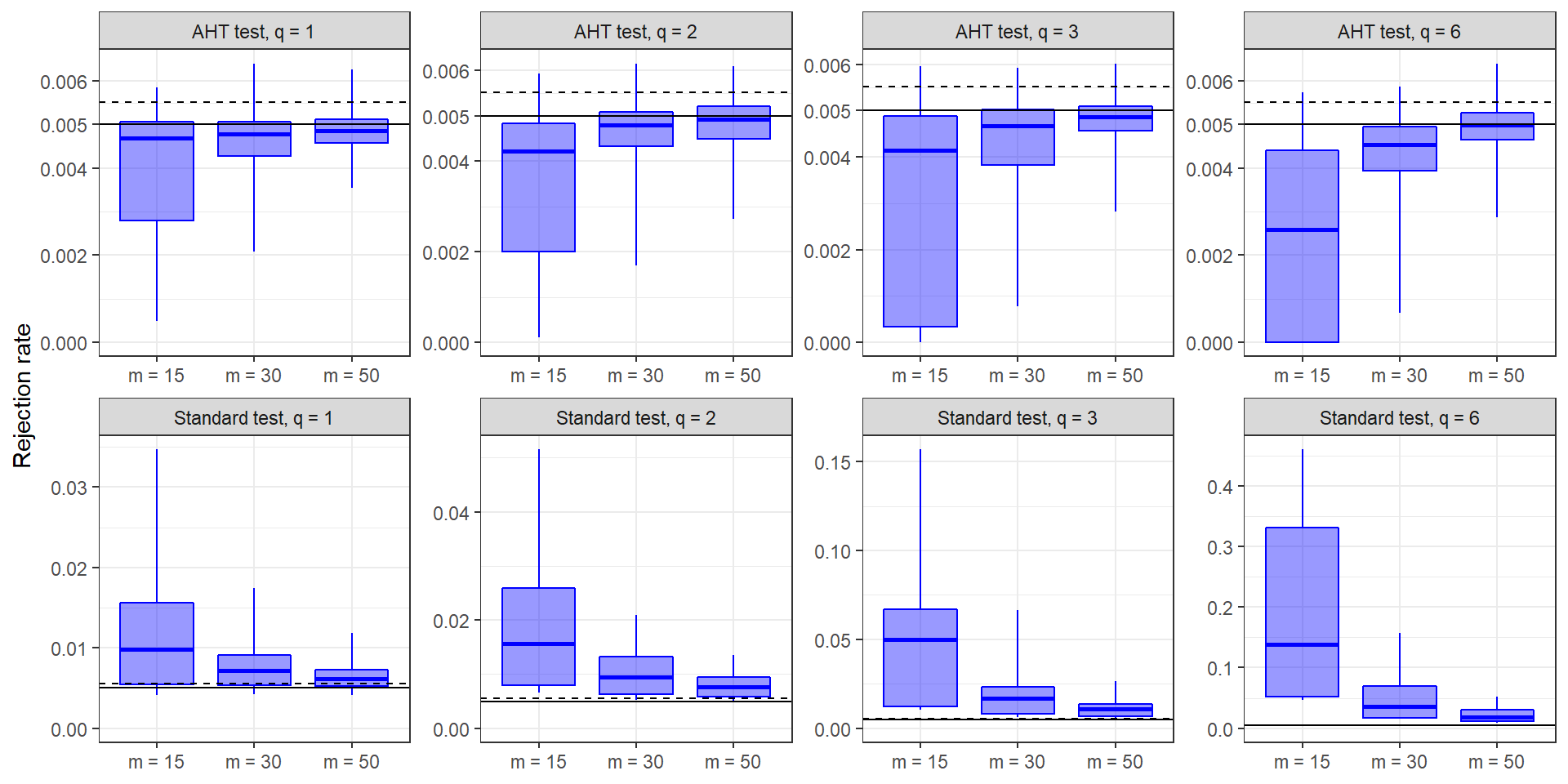
Rejection rates of AHT and standard tests for $\alpha=.05$, by dimension of hypothesis ($q$) and sample size ($m$). The solid horizontal line indicates the stated $\alpha$ level and the dashed line indicates an upper confidence bound on simulation error.

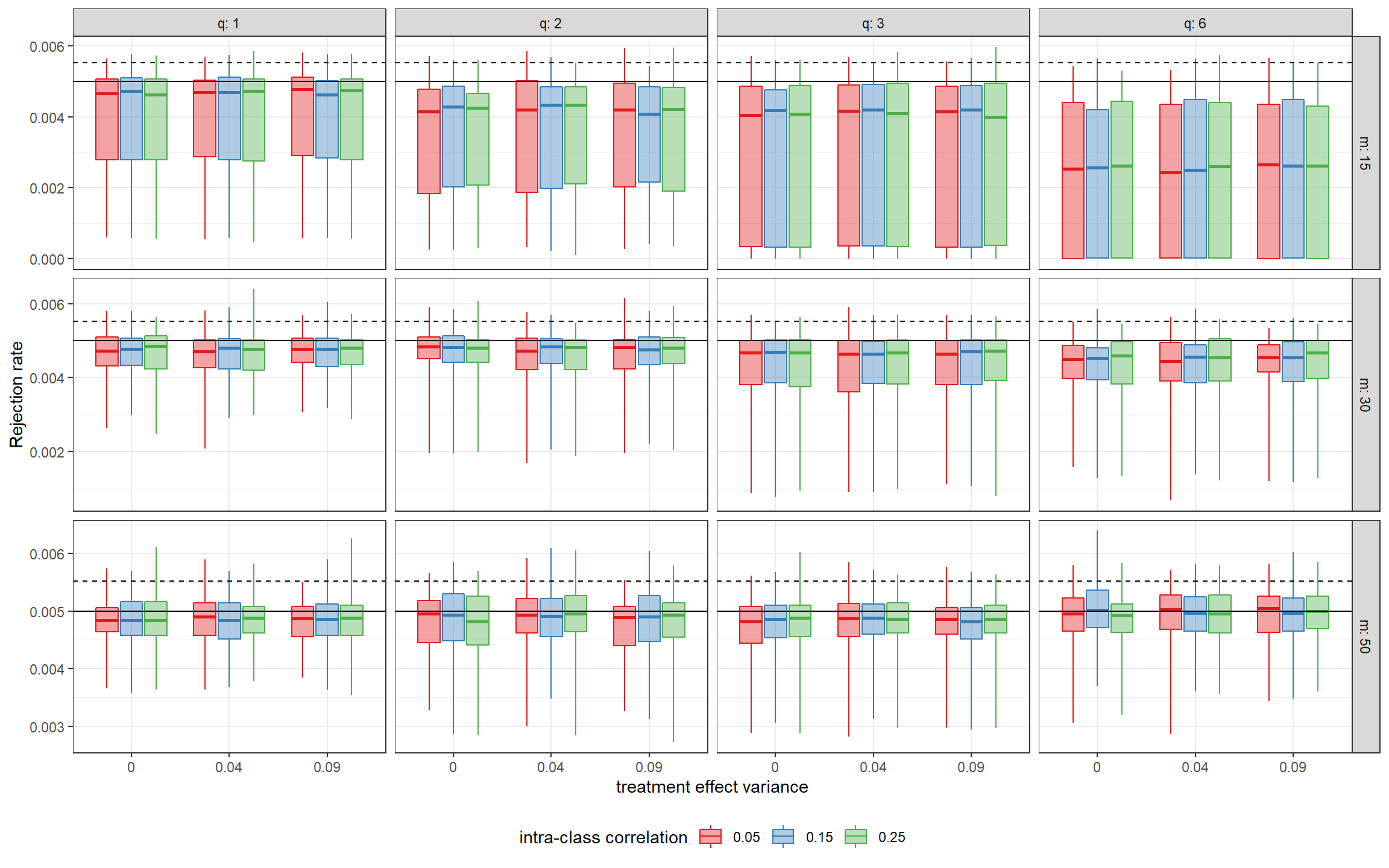
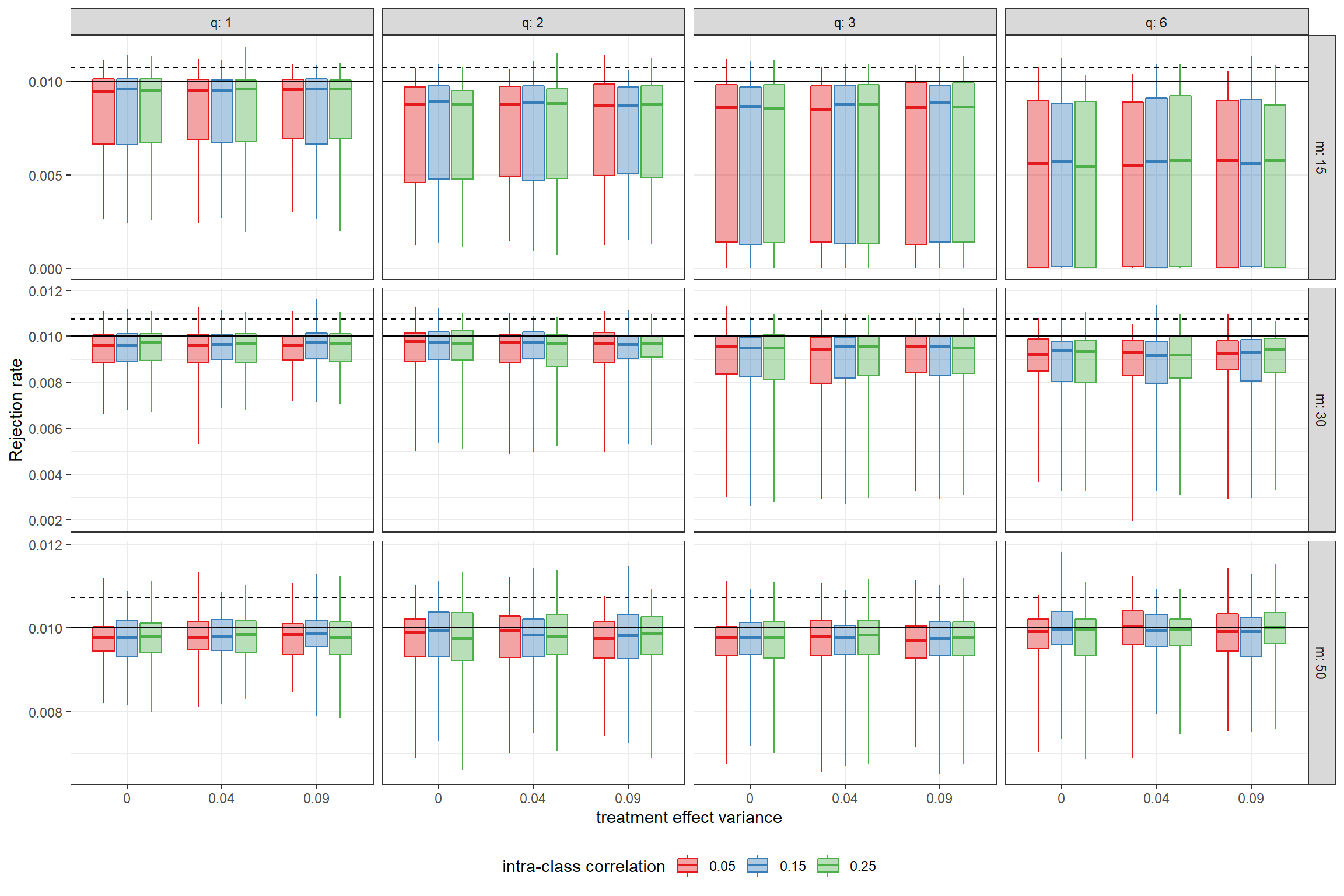
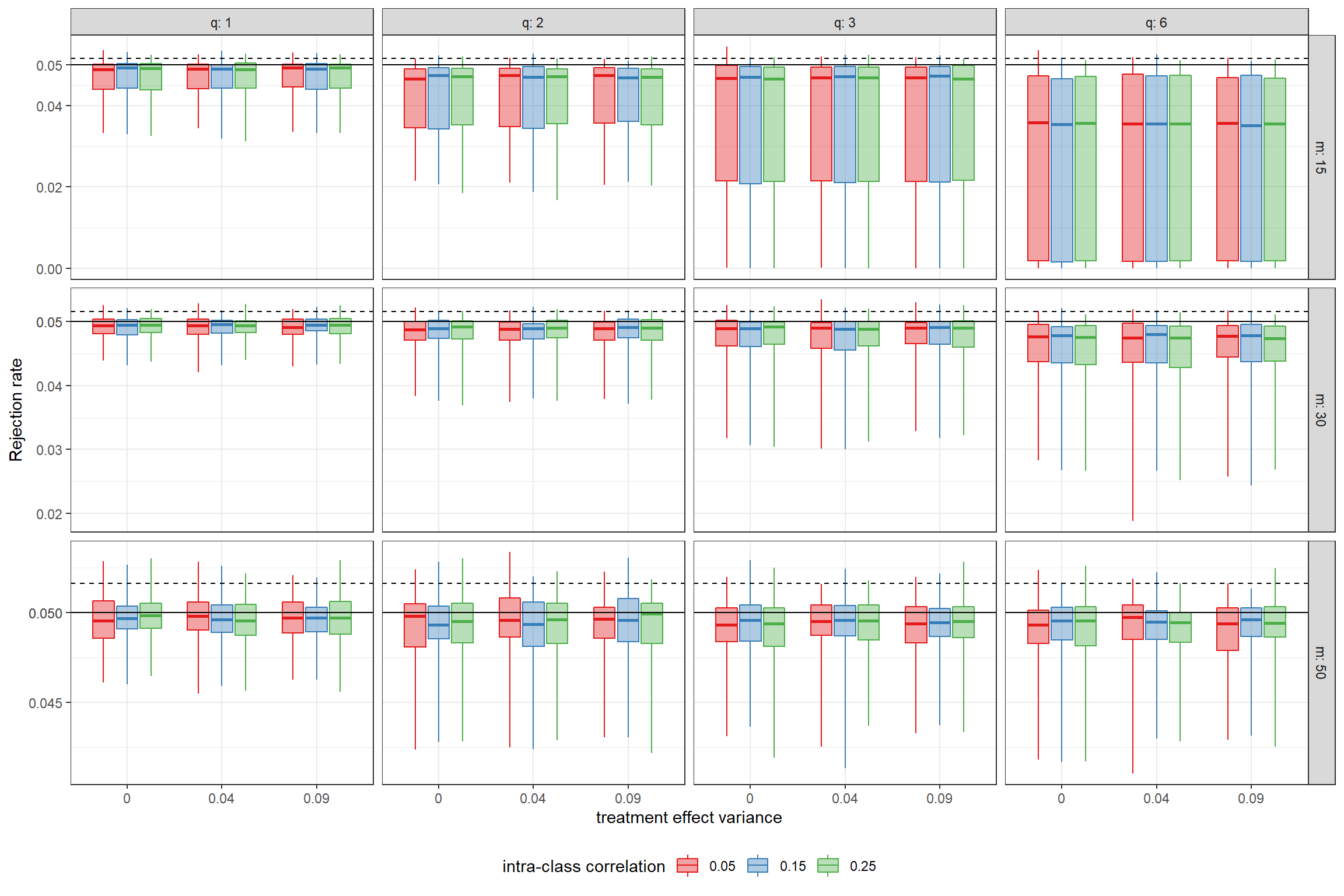
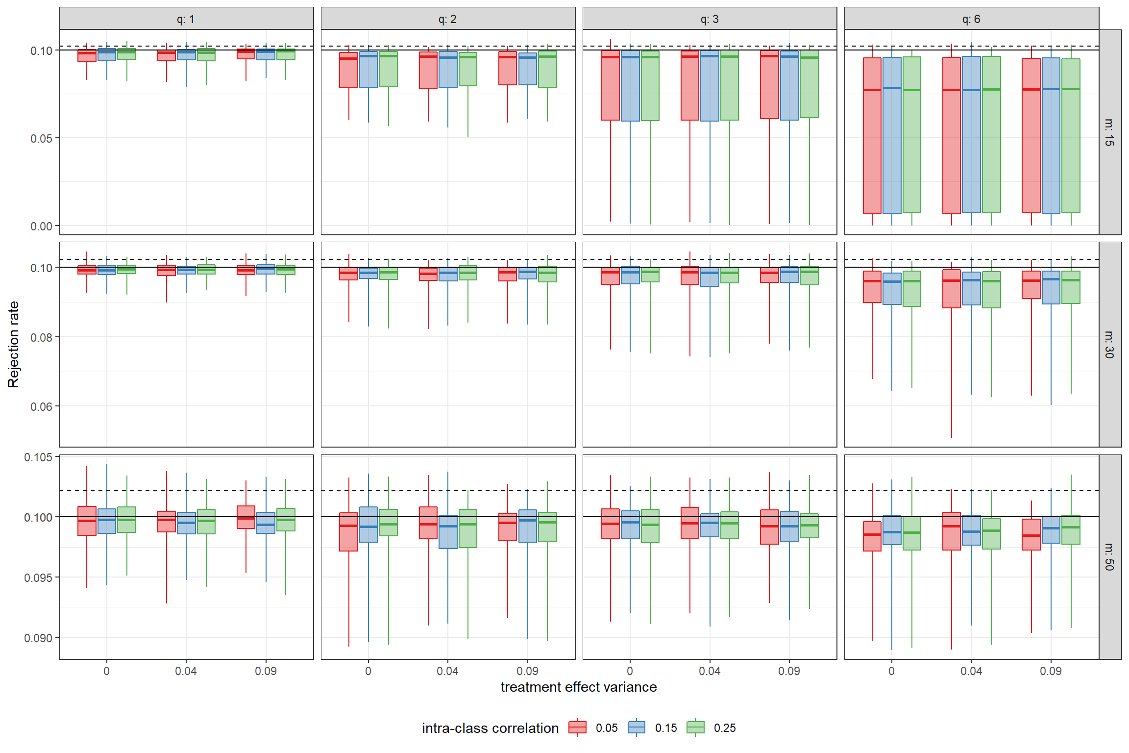
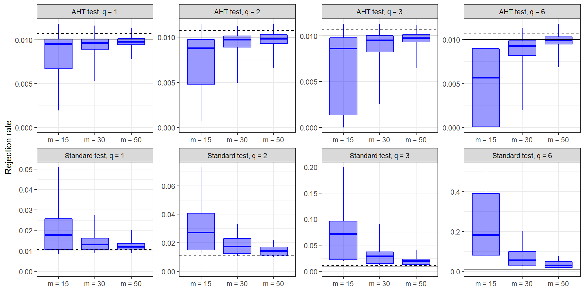
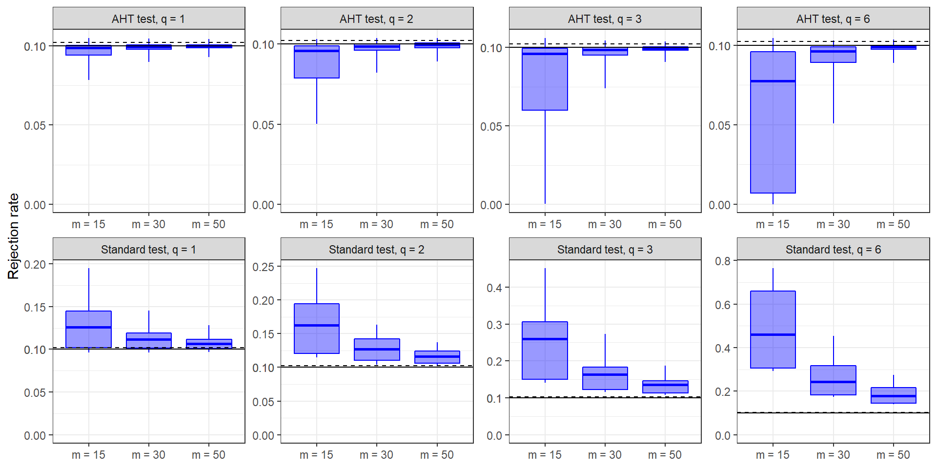
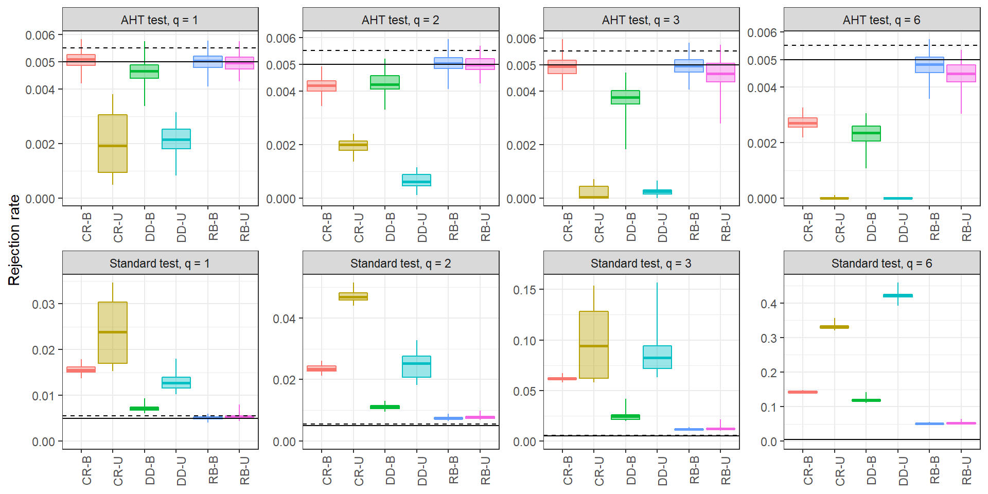
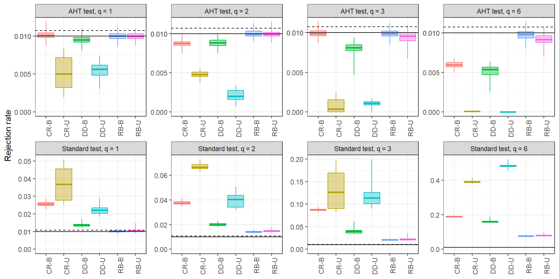
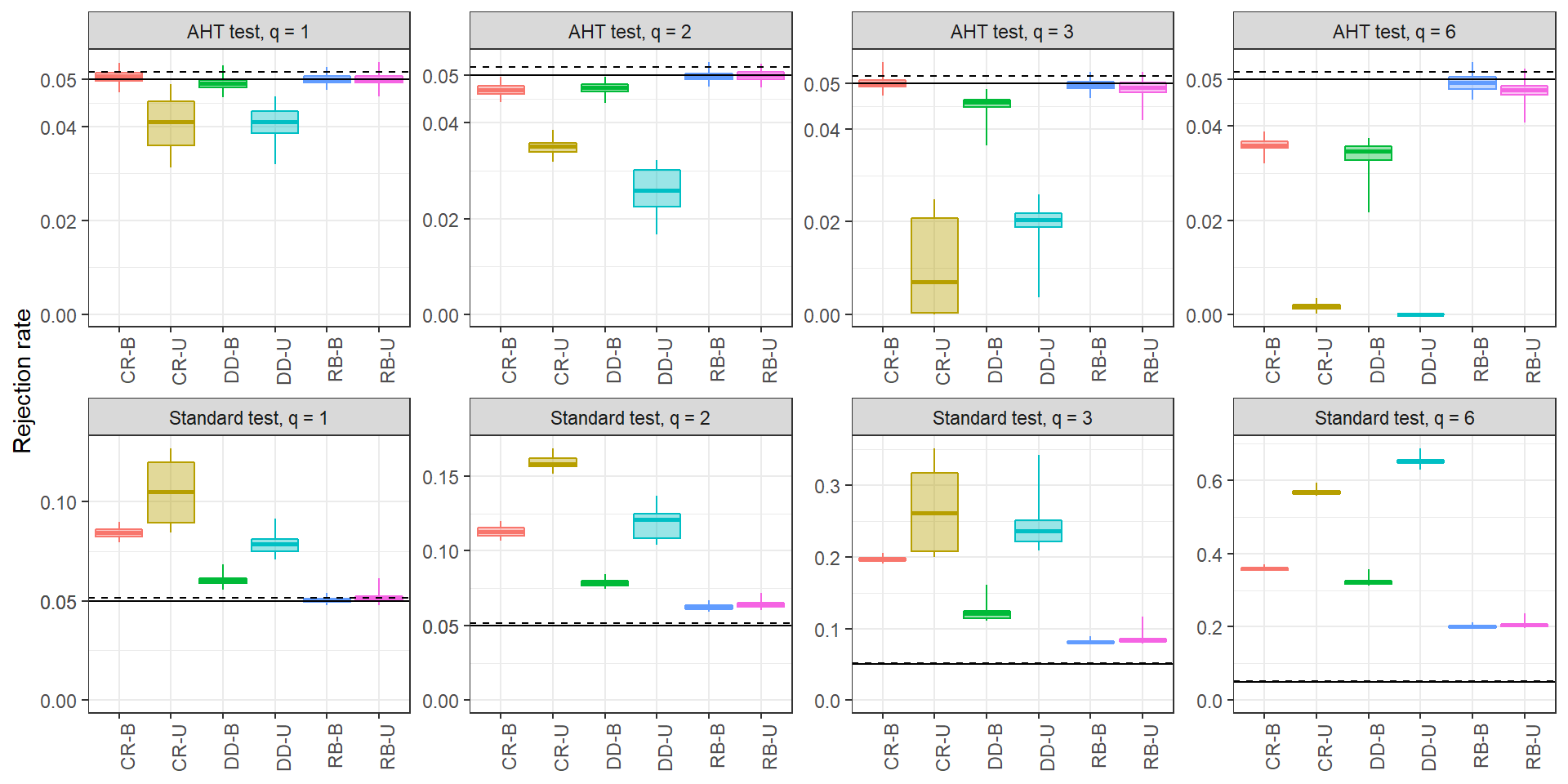
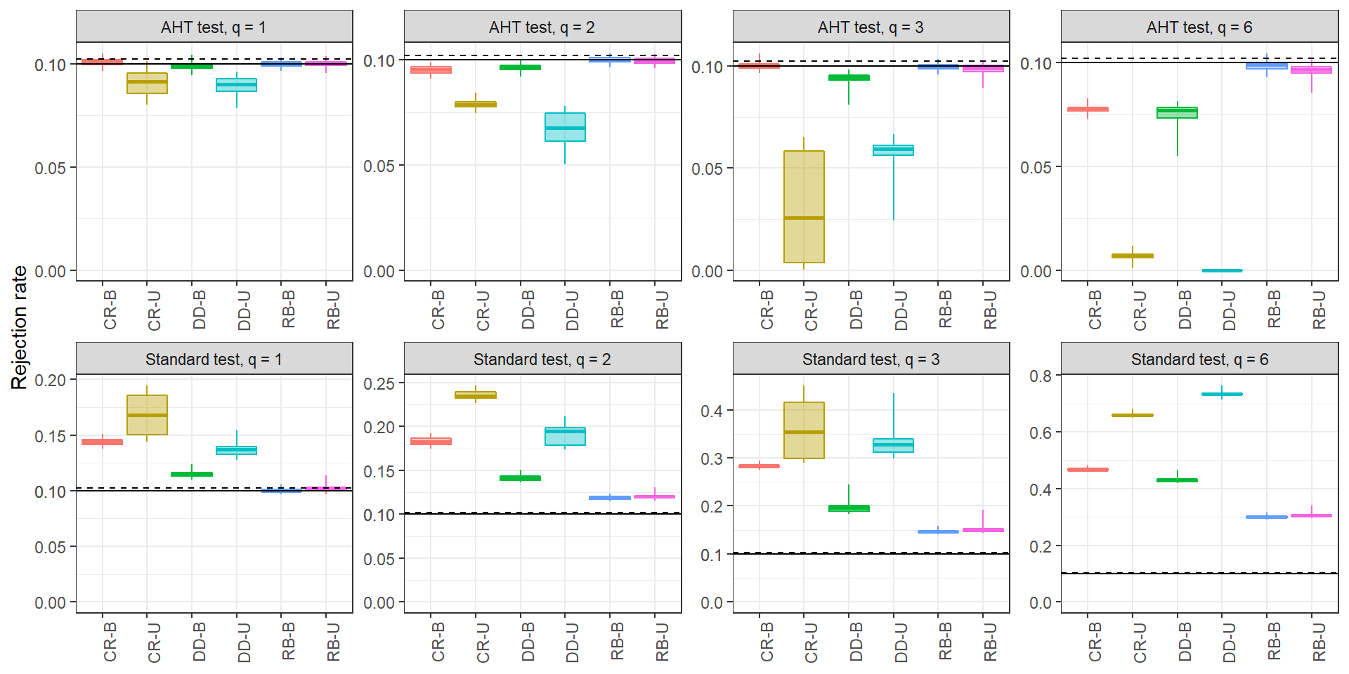
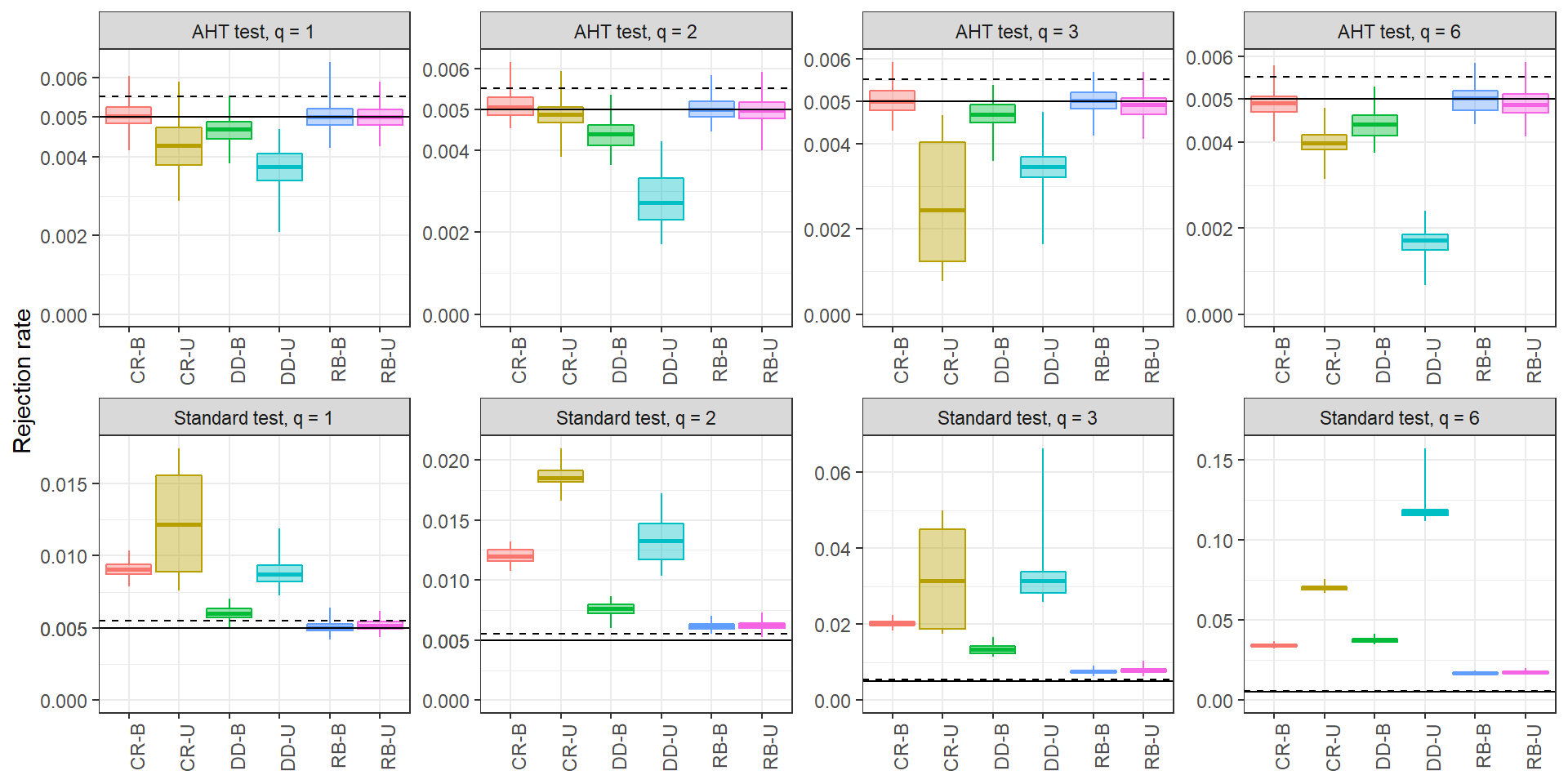
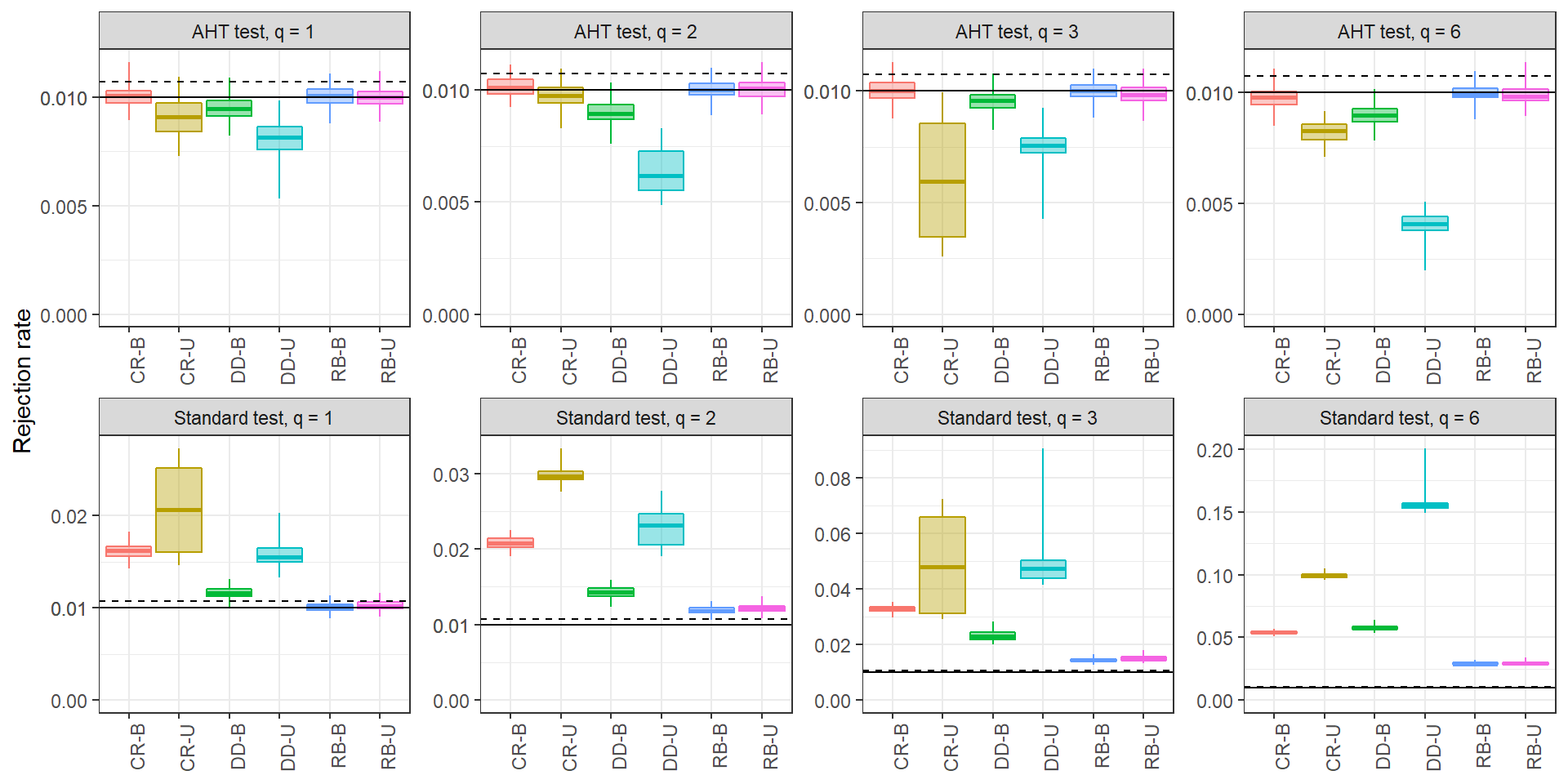
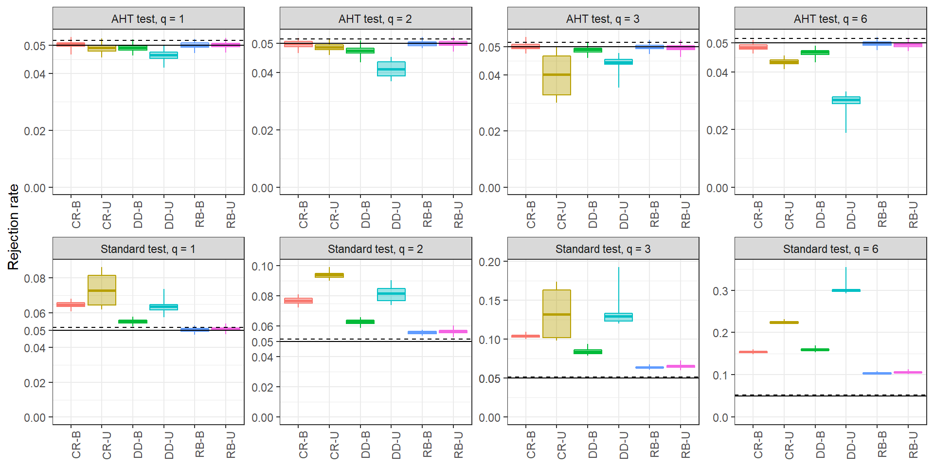
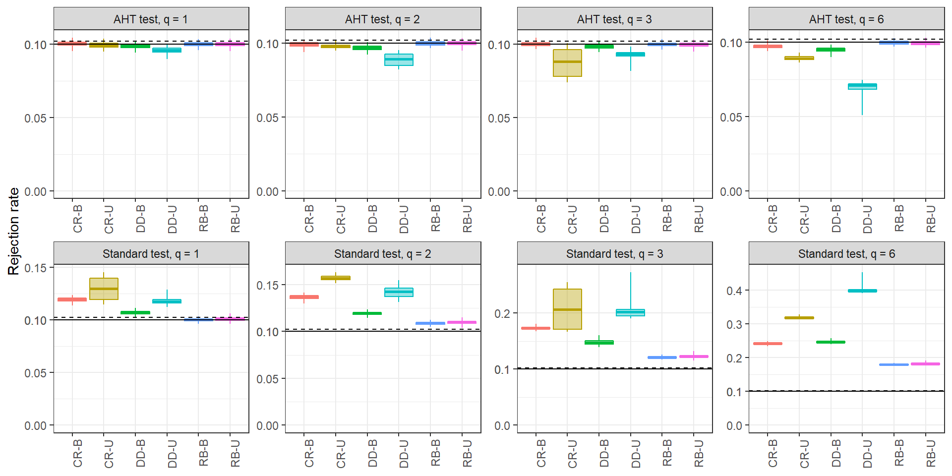
We discuss five main findings from the simulation results. Throughout, we present results for the nominal Type I error rate of $\alpha=.05$; results for other $\alpha$ levels are available in Appendix D. Supplementary materials include complete numerical results and replication code.

Overall performance.

The first finding is that the AHT test has Type I error close to the stated $\alpha$ level for all parameter combinations studied, whereas the standard test based on CR1 does not. Figure 4.2 illustrates this pattern at the nominal type I error rate of $\alpha=.05$, for constraints of varying dimension (from $q=1$, in the first column, to $q=6$, in the final column) and varying number of clusters. It can be seen that the AHT test nearly always has Type I error less than or equal to the stated $\alpha$ level, even with a small number of clusters. When the number of clusters is very small, the Type I error can be smaller than $\alpha$, particularly for tests of multiple-constraint hypotheses. Although the error is above the simulation bound under some conditions, the departures are typically small. For example, when $m=15$ the rejection rates do not exceed 0.012 for $\alpha=.01$, 0.055 for $\alpha=.05$, and 0.106 for $\alpha=.10$. The rejection rates are even closer to nominal for lower-dimensional constraints.

In comparison to the AHT test, the Type I error for the standard test can be markedly higher than the stated $\alpha$ level, particularly when the number of clusters is small or the dimension of the hypothesis is large. For example, the maximum Type I error ranges from 0.127 ($q=1$) to 0.687 ($q=6$) for data sets with 15 clusters. Perhaps even more important for practice, the rejection rate of the standard test can be far above the stated $\alpha$ level even when there are 50 clusters, with maximum error ranging from 0.071 ($q=1$) to 0.186 ($q=6$).

Rejection rates of AHT and standard tests, by study design and dimension of hypothesis ($q$) for $\alpha=.05$ and $m=30$. The solid horizontal line indicates the stated $\alpha$ level and the dashed line indicates an upper confidence bound on simulation error. CR = cluster-randomized design; DD = difference-in-differences design; RB = randomized block design; B = balanced; U = unbalanced.

Role of balance.

Figure 4.2 breaks out the rejection rates by study design, focusing on a sample size of $m=30$. In the bottom row, it can be seen that the rejection rate of the standard test increases with the dimension of the test ($q$) and the degree of unbalance in the study design. Differences between the balanced and unbalanced designs are largest for the CR and DD designs, with smaller discrepancies in RB designs. In the top row, rejection rates of the AHT test are near or below nominal (between 0.019 and 0.054) across all conditions with at least 30 clusters. Unbalanced designs lead to rejection rates that are usually below the nominal $\alpha$—just the opposite of how the standard test is affected by unbalance. This trend is the strongest for CR and DD designs. At the smallest sample size, the rejection rates of the AHT test are close to 0 in unbalanced CR and DD designs (see Appendix Figures A4-A7).

Figure 1: Range of denominator degrees of freedom for AHT test, by number of clusters and study design. CR = cluster-randomized design; DD = difference-in-differences design; RB = randomized block design; B = balanced; U = unbalanced.

Degrees of freedom.

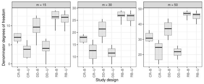
Figure 1 depicts the range of estimated degrees of freedom for the AHT test as a function of the study design and number of clusters ($m$). Within each box plot, the degrees of freedom vary depending on the hypothesis tested, with constraints of larger dimension having lower degrees of freedom. It can be seen that the AHT degrees of freedom are often far less than $m-1$ and that they are strongly affected by the pattern of treatment assignment and the degree of balance. The balanced and unbalanced RB designs have AHT degrees of freedom closest to $m-1$ because the treatment effects being tested are all identified within each cluster. The balanced DD design usually has the next largest degrees of freedom because it involves contrasts between two patterns of treatment configuration, followed by the balanced CR design, which involves contrasts between three patterns of treatment configurations. For both of these designs, unbalance leads to sharply reduced degrees of freedom.

Other correction factors.

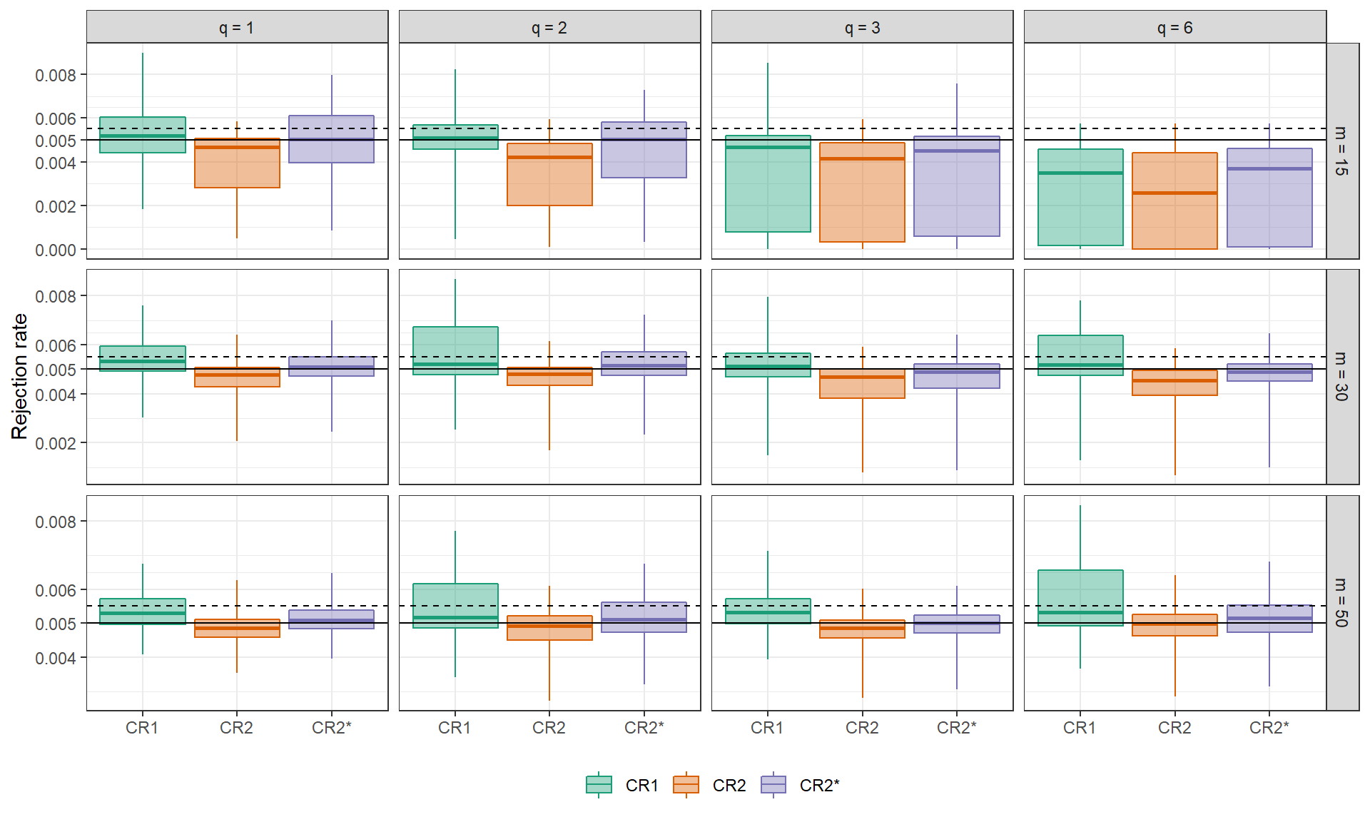
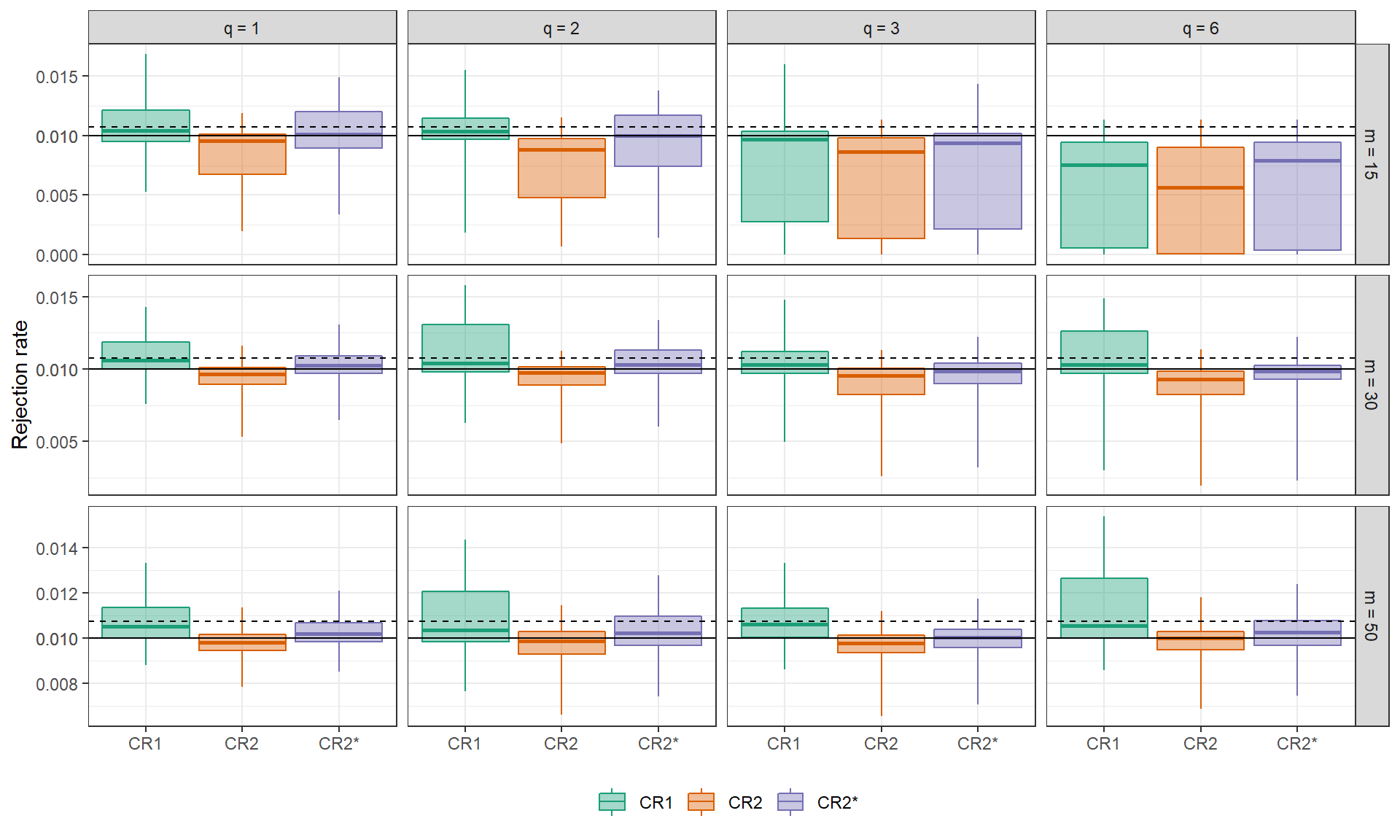
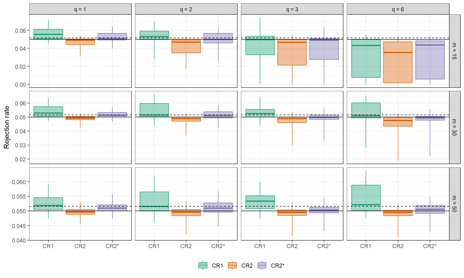
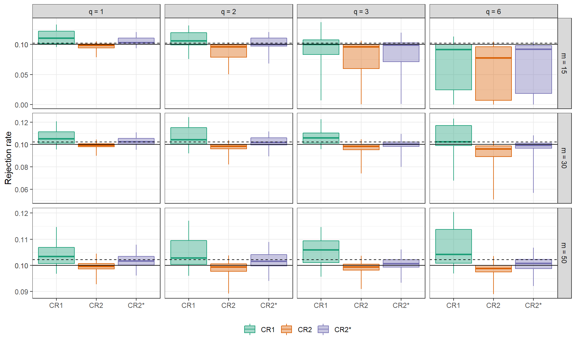
In principle, the AHT test could be applied with other forms of CRVEs, or could be calculated without accounting for absorption of the fixed effects. Appendix Figures A16 through A19 in the supplementary materials depict the rejection rates of two variants of the AHT test, including the test based on the CR1 adjustment matrices and the test based on CR2, but without accounting for absorption of fixed effects. Using the AHT degrees of freedom with the CR1 variance estimator leads to a drastic improvement compared to the standard test with $m-1$ degrees of freedom, although the rejection rates still exceed the nominal level under some conditions. The test based on CR2 without accounting for absorption has quite accurate rejection rates, although they exceed nominal levels more often than those of the test that does account for absorption, particularly for lower-dimensional hypotheses.

Misspecification.

By simulating the errors across a variety of parameter combinations, we were also able to test the impact of misspecification of the working model on Type I error. Because the CR2 correction and AHT degrees of freedom are both based on a working model with independent, homoskedastic errors, model misspecification increases with the true level of treatment effect variance ($\sigma_{\delta}^{2}$) and intra-class correlation ($\tau^{2}$). Across the nine error structures, the range of rejection rates remains very similar for the AHT test, with no clear pattern related to the degree of mis-specification (see Appendix Figures A20-A23). These findings follow closely those from Tipton and Pustejovsky (2015), which indicated that the Type I error of the AHT test was close to nominal even when the working model was quite discrepant from the data-generating model.

In summary, these results demonstrate that the standard robust Wald test, using the CR1 correction and $m-1$ degrees of freedom, produces a wide range of rejection rates, often far in excess of the nominal Type I error. In contrast, the rejection rates of the AHT tests are below or at most slightly above nominal, across all of the conditions examined. This is because the AHT test incorporates information about the covariate features into its estimated degrees of freedom, whereas the standard test does not. Compared to using the AHT test with the CR1 variance estimator or the modified CR2 estimator that ignores absorption of fixed effects, the AHT test based on CR2 leads to rejection rates that are closer to maintaining the nominal level, although the differences are often fairly small. An important question that remains is how much the standard test and AHT test diverge in actual application.

5 EXAMPLES

This section presents two examples that illustrate the performance of CRVE in different contexts. In the first example, the effects of substantive interest involve between-cluster contrasts. The second example involves a cluster-robust Hausman test for differences between within- and across-cluster information. In each example, we demonstrate the proposed AHT test for single- and multiple-parameter hypotheses and compare the results to the standard test based on the CR1 variance estimator and $m-1$ degrees of freedom. The focus here is on providing insight into the conditions under which the methods diverge in terms of three quantities of interest: the standard error estimates, the degrees of freedom estimates, and the stated p-values. Data files and replication code are available in the supplementary materials.

5.1 Achievement Awards demonstration

Angrist and Lavy (2009) reported results from a randomized trial in Israel that aimed to increase completion rates of the Bagrut, the national matriculation certificate for post-secondary education, among low-achieving high school students. In the Achievement Awards demonstration, 40 non-vocational high schools with low rates of Bagrut completion were selected from across Israel, including 10 Arab and 10 Jewish religious schools and 20 Jewish secular schools. The schools were then pair-matched based on 1999 rates of Bagrut completion, and within each pair one school was randomized to receive a cash-transfer program. In these treatment schools, seniors who completed certification were eligible for payments of approximately $1,500. Student-level covariate and outcome data were drawn from administrative records for the school years ending in June of 2000, 2001, and 2002. The incentive program was in effect for the group of seniors in treatment schools taking the Bagrut exams in Spring of 2001, but the program was discontinued for the following year. We therefore treat completion rates for 2000 and 2002 as being unaffected by treatment assignment. The primary outcome of interest is Bagrut completion.

This study involves relatively few clusters, with treatment assigned at the cluster level. For simplicity, we restrict our analysis to the sample of female students, which reduces the total sample to 35 schools. Following the original analysis of Angrist and Lavy (2009), we allow the program’s effects to vary depending on whether a students was in the upper or lower half of the distribution of prior-year academic performance. Letting $h=1,2,3$ index the sector of each school (Arab religious, Jewish religious, or Jewish secular), we consider the following analytic model:

$$y_{hitj}=z_{hit}\mathbf{r}_{hitj}^{\prime}\boldsymbol{\beta}_{h}+\mathbf{s}_{hitj}^{\prime}\boldsymbol{\gamma}+\gamma_{ht}+\mu_{i}+\epsilon_{hitj}$$ (16)

In this model for student $j$ in year $t$ in school $i$ in sector $h$, $z_{hit}$ is an indicator equal to one in the treatment schools for the 2001 school year and otherwise equal to zero; $\mathbf{r}_{hitj}$ is a vector of indicators for whether the student is in the lower or upper half of the distribution of prior academic performance; and $\boldsymbol{\beta}_{h}=\left(\beta_{1h},\beta_{2h}\right)$ is a vector of average treatment effects for schools in sector $h$. The vector $\mathbf{s}_{hitj}$ includes the following individual student demographic measures: mother’s and father’s education, immigration status, number of siblings, and indicators for each quartile in the distribution of prior-year academic performance. The model also includes fixed effects for each sector in each year ($\gamma_{ht}$) and for each school ($\mu_{i}$).

Based on Model (16), we test four hypotheses. First, we assume that the program effects are constant across sector (i.e., $\boldsymbol{\beta}_{1}=\boldsymbol{\beta}_{2}=\boldsymbol{\beta}_{3}=\boldsymbol{\beta}$) and test for whether the program affected completion rates for students in the upper half of the prior achievement distribution ($H_{0}:\beta_{2}=0$, with $q=1$). Second, we test for whether the program was effective in either half of the prior academic performance ($H_{0}:\boldsymbol{\beta}=0$, with $q=2$), still assuming that program effects are constant across sector. Third, we test for whether program effects in the upper half of the prior achievement distribution are moderated by school sector ($H_{0}:\beta_{21}=\beta_{22}=\beta_{23}$, with $q=3$). Finally, we conduct a joint test for whether program effects in either half of the prior achievement distribution are moderated by school sector ($H_{0}:\boldsymbol{\beta}_{1}=\boldsymbol{\beta}_{2}=\boldsymbol{\beta}_{3}$, with $q=4$).

Table 1: Tests of treatment effects in the Achievement Awards Demonstration

Hypothesis	Test	F	df	p
ATE - upper half (q = 1)	Standard	5.746	34.00	0.02217
	AHT	5.169	18.13	0.03539
ATE - joint (q = 2)	Standard	3.848	34.00	0.03116
	AHT	3.389	16.97	0.05775
Moderation - upper half (q = 2)	Standard	3.186	34.00	0.05393
	AHT	1.665	7.84	0.24959
Moderation - joint (q = 4)	Standard	8.213	34.00	0.00010
	AHT	3.091	3.69	0.16057

Table 1 reports the results of all four hypothesis tests. For the first two hypotheses, the AHT test statistics are slightly smaller than their standard counterparts and the degrees of freedom are considerably smaller. These differences in degrees of freedom arise because the treatment was assigned at the cluster level, while the subgroups varied within each cluster. In contrast, the AHT and standard tests diverge markedly for the third and fourth hypotheses tests, which compare treatment effects across sectors and subgroups. For these cases, the AHT test statistic and degrees of freedom are both considerably smaller than those from the standard test. This reflects the degree of unbalance in allocations across sectors (19 Jewish secular, 7 Jewish religious, and 9 Arab religious schools), combined with cluster-level randomization. In combination, these smaller test statistics and degrees of freedom result in larger p-values for the AHT test when compared to the standard test.

5.2 Effects of minimum legal drinking age on mortality

As a second illustration, we draw on a panel data analysis described in Angrist and Pischke (2014; see also Carpenter and Dobkin 2011). Based on data from the Fatal Accident Reporting System maintained by the National Highway Traffic Safety Administration, we estimate the effects of changes in the minimum legal drinking age over the time period of 1970-1983 on state-level death rates resulting from motor vehicle crashes. A standard difference-in-differences specification for such a state-by-year panel is

$$y_{it}=\mathbf{r}_{it}^{\prime}\boldsymbol{\beta}+\gamma_{t}+\mu_{i}+\epsilon_{it}.$$ (17)

In this model, time-point $t$ is nested within state $i$; the outcome $y_{it}$ is the number of deaths in motor vehicle crashes (per 100,000 residents) in state $i$ at time $t$; $\mathbf{r}_{it}$ is a vector of covariates; $\gamma_{t}$ is a fixed effect for time point $t$; and $\mu_{i}$ is an effect for state $i$. The vector $\mathbf{r}_{it}$ consists of a measure of the proportion of the population between the ages of 18 and 20 years who can legally drink alcohol and a measure of the beer taxation rate, both of which vary across states and across time.

We apply both random effects (RE) and fixed effects (FE) approaches to estimate the effect of lowering the legal drinking age. For the RE estimates, we use feasible GLS based the assumption that $\mu_{1},...,\mu_{m}$ are mutually independent, normally distributed, and independent of $\epsilon_{it}$ and $\mathbf{r}_{it}$. We also report an artificial Hausman test (Arellano 1993; Wooldridge 2010) for correlation between the covariates $\mathbf{r}_{it}$ and the state effects $\mu_{i}$. Such correlation creates bias in the RE estimator of the policy effect, thus necessitating the use of the FE estimator. The artificial Hausman test amends model (17) to include within-cluster deviations for the variables of interest, so that the specification becomes

$$y_{it}=\mathbf{r}_{it}\boldsymbol{\beta}+\mathbf{\ddot{r}}_{it}\boldsymbol{\delta}+\gamma_{t}+\mu_{i}+\epsilon_{it},$$ (18)

where $\mathbf{\ddot{r}}_{it}$ denotes the within-cluster deviations of the covariate. The parameter $\boldsymbol{\delta}$ captures the difference between the between-cluster and within-cluster estimates of $\boldsymbol{\beta}$. With this setup, the artificial Hausman test amounts to testing the null hypothesis that $\boldsymbol{\delta}=\mathbf{0}$, where $\boldsymbol{\delta}$ is estimated using RE.

Table 2: Tests of effects of minimum legal drink age and Hausman specification test

Hypothesis	Test	F	df	p
Random effects	Standard	8.261	49.00	0.00598
	AHT	7.785	26.69	0.00960
Fixed effects	Standard	9.660	49.00	0.00313
	AHT	9.116	24.58	0.00583
Hausman test	Standard	2.930	49.00	0.06283
	AHT	2.560	11.91	0.11886

Table 2 displays the results of the tests for the policy variable and the Hausman tests for each model specification. The results of the policy effect tests are quite similar across specifications and versions of the test. Of note is that, for both the RE and FE estimates, the AHT tests have only half the degrees of freedom of the corresponding standard tests. For the artificial Hausman test, the AHT test has fewer than 12 degrees of freedom, which leads to a much larger p-value compared to using the standard test based on CR1.

6 CONCLUSION

Empirical studies in economics often involve modeling data with a correlated error structure. In such applications, it is now routine to use cluster-robust variance estimation, which provides asymptotically valid standard errors and hypothesis tests without making strong parametric assumptions about the error structure. However, a growing body of recent work has drawn attention to the shortcomings of CRVE methods when the data include only a small or moderate number of independent clusters (Cameron, Gelbach, and Miller 2008; Cameron and Miller 2015; Imbens and Kolesar 2016; MacKinnon and Webb 2016). In particular, Wald tests based on CRVE can have rejection rates far in excess of the nominal Type I error. This problem is compounded by the fact that the performance of standard Wald tests depends on features of the study design beyond just the total number of clusters, which can make it difficult to determine whether standard, asymptotically valid CRVE methods are accurate.

One promising solution to this problem is to use the bias-reduced linearization variance estimator (i.e., CR2) proposed by Bell and McCaffrey (2002), which corrects the CRVE so that it is exactly unbiased under an analyst-specified working model for the error structure, together with degrees of freedom estimated based on the same working model. In this paper, we have extended the CR2 variance estimator so that it can be applied to test single- or multi-dimensional parameter constraints in models with fixed effects in multiple dimensions. We join Imbens and Kolesar (2016) in arguing that the CR2 estimator and corresponding estimated degrees of freedom for hypothesis tests should be applied routinely, whenever analysts use CRVE and hypothesis tests based thereon. Because the performance of standard CRVE methods depends on features of the study design, the total number of clusters in the data is an insufficient guide to whether small-sample corrections are needed. Instead, the clearest way to determine whether small-sample corrections are needed is simply to calculate them.

The idea of developing small-sample adjustments based on a working model may seem strange to analysts accustomed to using CRVE—after all, the whole point of clustering standard errors is to avoid making assumptions about the error structure. However, simulation studies reported here and elsewhere (Tipton 2015; Tipton and Pustejovsky 2015) have demonstrated that the approach is actually robust to a high degree of misspecification in the working model. Furthermore, while the working model provides necessary scaffolding when the number of clusters is small, its influence tends to fall away as the number of clusters increases, so that the CR2 estimator and AHT maintain the same asymptotic robustness as standard CRVE methods.

The proposed AHT test involves two adjustments: use of the CR2 adjustment for the variance estimator and use of estimated degrees of freedom. Our simulation results and empirical examples illustrate that the degrees of freedom adjustment has a relatively larger influence on small-sample performance. Even when used with the CR1 adjustment matrices, the degrees of freedom adjustment leads to much more accurate rejection rates, although using the CR2 estimator (and accounting for absorption of fixed effects) appears to be necessary to fully maintain the nominal level of the test. The approximate degrees of freedom of the AHT test can be much smaller than the number of clusters, particularly when the covariates involved in the test involve high leverage or are unbalanced across clusters. The estimated degrees of freedom are indicative of the precision of the standard errors, and thus provide diagnostic information that is similar to the effective sample size measure proposed by Carter, Schnepel, and Steigerwald (2013). We therefore recommend that the degrees of freedom be reported along with standard errors and $p$-values whenever the method is applied.

It is interesting to note that the consequences of accounting for fixed effects estimation with CR2 runs counter to how fixed effects enter into other small-sample corrections. In particular, including the fixed effect parameter dimension in the CR1S small sample adjustment can lead to bias when the per-cluster sample size is small (Cameron and Miller 2015), whereas accounting for the fixed effects with the CR2 estimator improves the accuracy of test rejection rates, although the difference is comparatively minor. Accounting for fixed effects also makes hypothesis test results invariant to how the regression is calculated (whether by LSDV or after absorption), which we see as a useful feature for ensuring the replicability of one’s analysis.

One limitation of our approach is that the rejection rates of the AHT tests tend to fall below nominal levels when the number of clusters is very small and the design is unbalanced. The under-rejection can be severe for tests of multi-dimensional constraints (e.g., $q=3$-dimensional hypotheses with $m=15$ clusters in an unbalanced difference-in-differences design). In principle, this problem could arise either because the proposed degrees of freedom estimator loses accuracy under these conditions or because the sampling distribution of the test statistic is no longer well-approximated by Hotelling’s $T^{2}$ distribution at all. In previous work, we investigated several other methods of approximating the degrees of freedom, but found none that were more accurate than the method describe in the present paper (Tipton and Pustejovsky 2015). Thus, future work may need to focus on other approximations to the reference distribution itself, such as an F distribution in which both the numerator and denominator degrees of freedom are estimated (cf. Mehrotra 1997) or computational approximations such as the cluster-wild bootstrap (MacKinnon and Webb 2016).

Another outstanding limitation of the CR2 variance estimator is that it is costly (or even infeasible) to compute when the within-cluster sample sizes are large (MacKinnon 2015). For example, Bertrand, Duflo, and Mullainathan (2004) analyzed micro-level data from a 21-year panel of current population survey data, with clustering by state. Their data included some state-level clusters with over $n_{i}=10,000$ individual observations. The CR2 adjustment matrices have dimension $n_{i}\times n_{i}$, and would be very expensive to compute in this application. Methods for improving the computational efficiency of the CR2 variance estimator (or alternative estimators that have similar performance to CR2), should be investigated further.

This paper has developed the CR2 estimator and AHT testing procedure for weighted least squares estimation of linear regression models. Extensions to linear regression models with clustering in multiple, non-nested dimensions (cf. Cameron, Gelbach, and Miller 2011) appear to be possible, and their utility should be further investigated. McCaffrey and Bell (2006) have proposed extensions to bias-reduced linearization for use with generalized estimating equations, and future work should consider further extensions to other classes of estimators, including two-stage least squares and generalized method of moments.

SUPPLEMENTARY MATERIALS

Supplementary materials for the simulation study and empirical examples are available at https://github.com/jepusto/clubSandwich/tree/main/paper_ClusterRobustTesting/R. The materials include R code for the simulation study, complete numerical results from the simulations, and data and R code for replicating the empirical examples.

REFERENCES

reAngrist, Joshua D, and Victor Lavy. 2009. “The effects of high stakes high school achievement awards : Evidence from a randomized trial.” American Economic Review 99 (4): 1384–414. https://doi.org/10.1257/aer.99.4.1384.

preAngrist, Joshua D, and Jörn-Steffen Pischke. 2014. Mastering’metrics: The Path from Cause to Effect. Princeton University Press.

preAngrist, Joshua D, and JS Pischke. 2009. Mostly harmless econometrics: An empiricist’s companion. Princeton, NJ: Princeton University Press.

preArellano, Manuel. 1987. “Computing robust standard errors for within-groups estimators.” Oxford Bulletin of Economics and Statistics 49 (4): 431–34.

pre———. 1993. “On the testing of correlated effects with panel data.” Journal of Econometrics 59 (1-2): 87–97. https://doi.org/10.1016/0304-4076(93)90040-C.

preBanerjee, Sudipto, and Anindya Roy. 2014. Linear Algebra and Matrix Analysis for Statistics. Boca Raton, FL: Taylor & Francis.

preBell, Robert M, and Daniel F McCaffrey. 2002. “Bias reduction in standard errors for linear regression with multi-stage samples.” Survey Methodology 28 (2): 169–81.

preBertrand, Marianne, Esther Duflo, and Sendhil Mullainathan. 2004. “How much should we trust differences-in-differences estimates?” Quarterly Journal of Economics 119 (1): 249–75.

preCai, Li, and Andrew F Hayes. 2008. “A new test of linear hypotheses in OLS regression under heteroscedasticity of unknown form.” Journal of Educational and Behavioral Statistics 33 (1): 21–40. https://doi.org/10.3102/1076998607302628.

preCameron, A Colin, Jonah B Gelbach, and Douglas Miller. 2008. “Bootstrap-based improvements for inference with clustered errors.” The Review of Economics and Statistics 90 (3): 414–27.

preCameron, A Colin, Jonah B Gelbach, and Douglas L Miller. 2011. “Robust inference with multiway clustering.” Journal of Business & Economic Statistics 29 (2): 238–49. https://doi.org/10.1198/jbes.2010.07136.

preCameron, A Colin, and Douglas L Miller. 2015. “A Practitioner’s Guide to Cluster-Robust Inference.” Journal of Human Resources 50 (2): 317–72. https://doi.org/10.3368/jhr.50.2.317.

preCarpenter, Christopher, and Carlos Dobkin. 2011. “The minimum legal drinking age and public health.” Journal of Economic Perspectives 25 (2): 133–56. https://doi.org/10.1257/jep.25.2.133.

preCarter, Andrew V, Kevin T Schnepel, and Douglas G Steigerwald. 2013. “Asymptotic Behavior of a t Test Robust to Cluster Heterogeneity.”

preConley, Timothy G, and Christopher R Taber. 2011. “Inference with ‘Difference in Differences’ with a Small Number of Policy Changes.” Review of Economics and Statistics 93 (1): 113–25.

preDavis, Peter. 2002. “Estimating multi-way error components models with unbalanced data structures.” Journal of Econometrics 106: 67–95. https://doi.org/10.1016/S0304-4076(01)00087-2.

preDonald, Stephen G, and Kevin Lang. 2007. “Inference with difference-in-differences and other panel data.” Review of Economics and Statistics 89 (2): 221–33. https://doi.org/10.1162/rest.89.2.221.

preFai, Alex. Hrong-Tai, and PL Cornelius. 1996. “Approximate F-tests of multiple degree of freedom hypotheses in generalized least squares analyses of unbalanced split-plot experiments.” Journal of Statistical Computation and Simulation 54 (4): 363–78.

preHansen, Christian B. 2007. “Asymptotic properties of a robust variance matrix estimator for panel data when T is large.” Journal of Econometrics 141: 597–620. https://doi.org/10.1016/j.jeconom.2006.10.009.

preIbragimov, Rustam, and Ulrich K Müller. 2010. “t-Statistic based correlation and heterogeneity robust inference.” Journal of Business & Economic Statistics 28 (4): 453–68. https://doi.org/10.1198/jbes.2009.08046.

pre———. 2016. “Inference with few heterogeneous clusters.” Review of Economics and Statistics 98 (1): 83–96. https://doi.org/10.1162/REST_a_00545.

preImbens, Guido W, and Michal Kolesar. 2016. “Robust Standard Errors in Small Samples: Some Practical Advice.” Review of Economics and Statistics forthcoming.

preKrishnamoorthy, K, and Jianqi Yu. 2004. “Modified Nel and Van der Merwe test for the multivariate Behrens–Fisher problem.” Statistics & Probability Letters 66 (2): 161–69. https://doi.org/10.1016/j.spl.2003.10.012.

preLee, David S, and David Card. 2008. “Regression discontinuity inference with specification error.” Journal of Econometrics 142 (2): 655–74. https://doi.org/10.1016/j.jeconom.2007.05.003.

preLiang, Kung-Yee, and Scott L Zeger. 1986. “Longitudinal data analysis using generalized linear models.” Biometrika 73 (1): 13–22.

preMacKinnon, James G. 2013. “Thirty years of heteroskedasticity-robust inference.” In Recent Advances and Future Directions in Causality, Prediction, and Specification Analysis, edited by Xiaohong Chen and Norman R. Swanson. New York, NY: Springer New York. https://doi.org/10.1007/978-1-4614-1653-1.

pre———. 2015. “Wild cluster bootstrap confidence intervals.” L’Actualite Economique, Revue d’analyse Economique 91 (1-2): 11–33.

preMacKinnon, James G, and Matthew D Webb. 2016. “Wild bootstrap inference for wildly different cluster sizes.” Journal of Applied Econometrics forthcoming. https://doi.org/10.1002/jae.2508.

preMacKinnon, James G, and Halbert White. 1985. “Some heteroskedasticity-consistent covariance matrix estimators with improved finite sample properties.” Journal of Econometrics 29: 305–25.

preMancl, Lloyd A, and Timothy A DeRouen. 2001. “A covariance estimator for GEE with improved small-sample properties.” Biometrics 57 (1): 126–34.

preMcCaffrey, Daniel F, and Robert M Bell. 2006. “Improved hypothesis testing for coefficients in generalized estimating equations with small samples of clusters.” Statistics in Medicine 25 (23): 4081–98. https://doi.org/10.1002/sim.2502.

preMcCaffrey, Daniel F, Robert M Bell, and Carsten H Botts. 2001. “Generalizations of biased reduced linearization.” In Proceedings of the Annual Meeting of the American Statistical Association. 1994.

preMehrotra, Devan V. 1997. “Improving the brown-forsythe solution to the generalized behrens-fisher problem.” Communications in Statistics - Simulation and Computation 26 (3): 1139–45. https://doi.org/10.1080/03610919708813431.

preNel, D G, and C A van der Merwe. 1986. “A solution to the multivariate Behrens-Fisher problem.” Communications in Statistics - Theory and Methods 15 (12): 3719–35.

prePan, Wei, and Melanie M Wall. 2002. “Small-sample adjustments in using the sandwich variance estimator in generalized estimating equations.” Statistics in Medicine 21 (10): 1429–41. https://doi.org/10.1002/sim.1142.

preSatterthwaite, Franklin E. 1946. “An approximate distribution of estimates of variance components.” Biometrics Bulletin 2 (6): 110–14.

preTipton, Elizabeth. 2015. “Small sample adjustments for robust variance estimation with meta-regression.” Psychological Methods 20 (3): 375–93. https://doi.org/10.1037/met0000011.

preTipton, Elizabeth, and James E Pustejovsky. 2015. “Small-sample adjustments for tests of moderators and model fit using robust variance estimation in meta-regression.” Journal of Educational and Behavioral Statistics 40 (6): 604–34.

preWhite, Halbert. 1984. Asymptotic Theory for Econometricians. Orlando, FL: Academic Press, Inc.

preWooldridge, Jeffrey M. 2003. “Cluster-sample methods in applied econometrics.” The American Economic Review 93 (2): 133–38.

pre———. 2010. Econometric Analysis of Cross Section and Panel Data. 2nd ed. Cambridge, MA: MIT Press.

preYoung, Alwyn. 2016. “Improved, nearly exact, statistical inference with robust and clustered covariance matrices using effective degrees of freedom corrections.” London School of Economics. http://personal.lse.ac.uk/YoungA/Improved.pdf.

preZhang, Jin-Ting. 2012. “An approximate degrees of freedom test for heteroscedastic two-way ANOVA.” Journal of Statistical Planning and Inference 142 (1): 336–46. https://doi.org/10.1016/j.jspi.2011.07.023.

p

Appendix A Proof of Theorem 1

Consider the matrix $\mathbf{B}_{i}$ as defined in (8):

$$\mathbf{B}_{i}=\mathbf{D}_{i}\left(\mathbf{I}-\mathbf{H_{X}}\right)_{i}\boldsymbol{\Phi}\left(\mathbf{I}-\mathbf{H_{X}}\right)_{i}^{\prime}\mathbf{D}_{i}^{\prime},$$

The Moore-Penrose inverse of $\mathbf{B}_{i}$ can be computed from its eigen-decomposition. Let $b\leq n_{i}$ denote the rank of $\mathbf{B}_{i}$. Let $\boldsymbol{\Lambda}$ be the $b\times b$ diagonal matrix of the positive eigenvalues of $\mathbf{B}_{i}$ and $\mathbf{V}$ be the $n_{i}\times b$ matrix of corresponding eigen-vectors, so that $\mathbf{B}_{i}=\mathbf{V}\boldsymbol{\Lambda}\mathbf{V}^{\prime}$. Then $\mathbf{B}_{i}^{+}=\mathbf{V}\boldsymbol{\Lambda}^{-1}\mathbf{V}^{\prime}$ and $\mathbf{B}_{i}^{+1/2}=\mathbf{V}\boldsymbol{\Lambda}^{-1/2}\mathbf{V}^{\prime}$. Because the adjustment matrices taken to be $\mathbf{A}_{i}=\mathbf{D}_{i}^{\prime}\mathbf{B}_{i}^{+1/2}\mathbf{D}_{i}$, we have that

$$\mathbf{\ddot{R}}_{i}^{\prime}\mathbf{W}_{i}\mathbf{A}_{i}\left(\mathbf{I}-\mathbf{H_{X}}\right)_{i}\boldsymbol{\Phi}\left(\mathbf{I}-\mathbf{H_{X}}\right)_{i}^{\prime}\mathbf{A}_{i}^{\prime}\mathbf{W}_{i}\mathbf{\ddot{R}}_{i} =\mathbf{\ddot{R}}_{i}^{\prime}\mathbf{W}_{i}\mathbf{D}_{i}^{\prime}\mathbf{B}_{i}^{+1/2}\mathbf{B}_{i}\mathbf{B}_{i}^{+1/2}\mathbf{D}_{i}\mathbf{W}_{i}\mathbf{\ddot{R}}_{i}$$ (A1)

$$=\mathbf{\ddot{R}}_{i}^{\prime}\mathbf{W}_{i}\mathbf{D}_{i}^{\prime}\mathbf{V}\mathbf{V}^{\prime}\mathbf{D}_{i}\mathbf{W}_{i}\mathbf{\ddot{R}}_{i}.$$

Thus, it will suffice to show that $\mathbf{V}^{\prime}\mathbf{D}_{i}\mathbf{W}_{i}\mathbf{\ddot{R}}_{i}=\mathbf{D}_{i}\mathbf{W}_{i}\mathbf{\ddot{R}}_{i}$.

Now, because $\mathbf{D}_{i}$ and $\boldsymbol{\Phi}$ are positive definite and $\mathbf{B}_{i}$ is symmetric, the eigen-vectors $\mathbf{V}$ define an orthonormal basis for the column span of $\left(\mathbf{I}-\mathbf{H_{X}}\right)_{i}$. We now show that $\mathbf{\ddot{U}}_{i}$ is in the column space of $\left(\mathbf{I}-\mathbf{H_{X}}\right)_{i}$. Let $\mathbf{Z}_{i}$ be an $n_{i}\times(r+s)$ matrix of zeros. With $\mathbf{L}_{i}$ as defined in Theorem 1, take $\mathbf{Z}_{k}=-\mathbf{\ddot{U}}_{k}\mathbf{L}_{i}^{-1}\mathbf{M}_{\mathbf{\ddot{U}}}^{-1}$, for $k\neq i$ and $\mathbf{Z}=\left(\mathbf{Z}_{1}^{\prime},...,\mathbf{Z}_{m}^{\prime}\right)^{\prime}$. Observe that $\left(\mathbf{I}-\mathbf{H_{T}}\right)\mathbf{Z}=\mathbf{Z}$. It follows that

$$\left(\mathbf{I}-\mathbf{H_{X}}\right)_{i}\mathbf{Z} =\left(\mathbf{I}-\mathbf{H_{\ddot{U}}}\right)_{i}\left(\mathbf{I}-\mathbf{H_{T}}\right)\mathbf{Z}$$

$$=\left(\mathbf{I}-\mathbf{H_{\ddot{U}}}\right)_{i}\mathbf{Z}$$

$$=\mathbf{Z}_{i}-\mathbf{\ddot{U}}_{i}\mathbf{M_{\ddot{U}}}\sum_{k=1}^{m}\mathbf{\ddot{U}}_{k}^{\prime}\mathbf{W}_{k}\mathbf{Z}_{k}$$

$$=\mathbf{\ddot{U}}_{i}\mathbf{M_{\ddot{U}}}\left(\sum_{k\neq i}\mathbf{\ddot{U}}_{k}^{\prime}\mathbf{W}_{k}\mathbf{\ddot{U}}\right)\mathbf{L}_{i}^{-1}\mathbf{M}_{\mathbf{\ddot{U}}}^{-1}$$

$$=\mathbf{\ddot{U}}_{i}\mathbf{M_{\ddot{U}}}\mathbf{L}_{i}\mathbf{L}_{i}^{-1}\mathbf{M}_{\mathbf{\ddot{U}}}^{-1}$$

$$=\mathbf{\ddot{U}}_{i}.$$

Thus, there exists an $N\times(r+s)$ matrix $\mathbf{Z}$ such that $\left(\mathbf{I}-\mathbf{H_{\ddot{X}}}\right)_{i}\mathbf{Z}=\mathbf{\ddot{U}}_{i}$, i.e., $\mathbf{\ddot{U}}_{i}$ is in the column span of $\left(\mathbf{I}-\mathbf{H_{X}}\right)_{i}$. Because $\mathbf{D}_{i}\mathbf{W}_{i}$ is positive definite and $\mathbf{\ddot{R}}_{i}$ is a sub-matrix of $\mathbf{\ddot{U}}_{i}$, $\mathbf{D}_{i}\mathbf{W}_{i}\mathbf{\ddot{R}}_{i}$ is also in the column span of $\left(\mathbf{I}-\mathbf{H_{X}}\right)_{i}$. It follows that

$$\mathbf{\ddot{R}}_{i}^{\prime}\mathbf{W}_{i}\mathbf{D}_{i}^{\prime}\mathbf{V}\mathbf{V}^{\prime}\mathbf{D}_{i}\mathbf{W}_{i}\mathbf{\ddot{R}}_{i}=\mathbf{\ddot{R}}_{i}^{\prime}\mathbf{W}_{i}\boldsymbol{\Phi}_{i}\mathbf{W}_{i}\mathbf{\ddot{R}}_{i}.$$ (A2)

Substituting (A2) into (A1) demonstrates that $\mathbf{A}_{i}$ satisfies the generalized BRL criterion (Equation 6 of the main text).

Under the working model, the residuals from cluster $i$ have mean $\mathbf{0}$ and variance

$$\text{Var}\left(\mathbf{\ddot{e}}_{i}\right)=\left(\mathbf{I}-\mathbf{H_{X}}\right)_{i}\boldsymbol{\Phi}\left(\mathbf{I}-\mathbf{H_{X}}\right)_{i}^{\prime},$$

It follows that

$$\text{E}\left(\mathbf{V}^{CR2}\right) =\mathbf{M_{\ddot{R}}}\left[\sum_{i=1}^{m}\mathbf{\ddot{R}}_{i}^{\prime}\mathbf{W}_{i}\mathbf{A}_{i}\left(\mathbf{I}-\mathbf{H_{X}}\right)_{i}\boldsymbol{\Phi}\left(\mathbf{I}-\mathbf{H_{X}}\right)_{i}^{\prime}\mathbf{A}_{i}\mathbf{W}_{i}\mathbf{\ddot{R}}_{i}\right]\mathbf{M_{\ddot{R}}}$$

$$=\mathbf{M_{\ddot{R}}}\left[\sum_{i=1}^{m}\mathbf{\ddot{R}}_{i}^{\prime}\mathbf{W}_{i}\boldsymbol{\Phi}_{i}\mathbf{W}_{i}\mathbf{\ddot{R}}_{i}\right]\mathbf{M_{\ddot{R}}}$$

$$=\text{Var}\left(\boldsymbol{\hat{\beta}}\right)$$

Appendix B Proof of Theorem 2

If $\mathbf{W}_{i}=\boldsymbol{\Phi}_{i}=\mathbf{I}_{i}$, then we can write $\mathbf{B}_{i}$ from Equation (8) as

$$\mathbf{B}_{i} =\mathbf{D}_{i}\left(\mathbf{I}-\mathbf{H_{\ddot{U}}}\right)_{i}\left(\mathbf{I}-\mathbf{H_{T}}\right)\boldsymbol{\Phi}\left(\mathbf{I}-\mathbf{H_{T}}\right)^{\prime}\left(\mathbf{I}-\mathbf{H_{\ddot{U}}}\right)_{i}^{\prime}\mathbf{D}_{i}^{\prime}$$

$$=\left(\mathbf{I}-\mathbf{H_{\ddot{U}}}-\mathbf{H_{T}}\right)_{i}\left(\mathbf{I}-\mathbf{H_{\ddot{U}}}-\mathbf{H_{T}}\right)_{i}^{\prime}$$

$$=\left(\mathbf{I}_{i}-\mathbf{\ddot{U}}_{i}\mathbf{M_{\ddot{U}}}\mathbf{\ddot{U}}_{i}^{\prime}-\mathbf{T}_{i}\mathbf{M_{T}}\mathbf{T}_{i}^{\prime}\right),$$ (A3)

where the last equality follows from the fact that $\mathbf{\ddot{U}}_{i}^{\prime}\mathbf{T}_{i}=\mathbf{0}$ for $i=1,...,m$. Similarly, we can write

$$\tilde{\mathbf{B}}_{i}=\left(\mathbf{I}_{i}-\mathbf{\ddot{U}}_{i}\mathbf{M_{\ddot{U}}}\mathbf{\ddot{U}}_{i}^{\prime}\right).$$ (A4)

We now show that $\tilde{\mathbf{A}}_{i}\mathbf{T}_{i}=\mathbf{T}_{i}$. Denote the rank of $\mathbf{\ddot{U}}_{i}$ as $u_{i}\leq\min\left\{n_{i},r+s\right\}$ and take the thin QR decomposition of $\mathbf{\ddot{U}}_{i}$ as $\mathbf{\ddot{U}}_{i}=\mathbf{Q}_{i}\mathbf{R}_{i}$, where $\mathbf{Q}_{i}$ is an $n_{i}\times u_{i}$ semi-orthonormal matrix and $\mathbf{R}_{i}$ is a $u_{i}\times r+s$ matrix of rank $u_{i}$, with $\mathbf{Q}_{i}^{\prime}\mathbf{Q}_{i}=\mathbf{I}$. Note that $\mathbf{Q}_{i}^{\prime}\mathbf{T}_{i}=\mathbf{0}$. From the observation that $\tilde{\mathbf{B}}_{i}$ can be written as

$$\tilde{\mathbf{B}}_{i}=\mathbf{I}_{i}-\mathbf{Q}_{i}\mathbf{Q}_{i}^{\prime}+\mathbf{Q}_{i}\left(\mathbf{I}-\mathbf{R}_{i}\mathbf{M}_{\mathbf{\ddot{U}}}\mathbf{R}_{i}^{\prime}\right)\mathbf{Q}_{i}^{\prime},$$

it can be seen that

$$\tilde{\mathbf{A}}_{i}=\tilde{\mathbf{B}}_{i}^{+1/2}=\mathbf{I}_{i}-\mathbf{Q}_{i}\mathbf{Q}_{i}^{\prime}+\mathbf{Q}_{i}\left(\mathbf{I}-\mathbf{R}_{i}\mathbf{M}_{\mathbf{\ddot{U}}}\mathbf{R}_{i}^{\prime}\right)^{+1/2}\mathbf{Q}_{i}^{\prime}.$$ (A5)

It follows that $\tilde{\mathbf{A}}_{i}\mathbf{T}_{i}=\mathbf{T}_{i}$.

Setting

$$\mathbf{A}_{i}=\tilde{\mathbf{A}}_{i}-\mathbf{T}_{i}\mathbf{M_{T}}\mathbf{T}_{i}^{\prime},$$ (A6)

observe that

$$\mathbf{B}_{i}\mathbf{A}_{i}\mathbf{B}_{i}\mathbf{A}_{i} =\left(\tilde{\mathbf{B}}_{i}-\mathbf{T}_{i}\mathbf{M_{T}}\mathbf{T}_{i}^{\prime}\right)\left(\tilde{\mathbf{A}}_{i}-\mathbf{T}_{i}\mathbf{M_{T}}\mathbf{T}_{i}^{\prime}\right)\left(\tilde{\mathbf{B}}_{i}-\mathbf{T}_{i}\mathbf{M_{T}}\mathbf{T}_{i}^{\prime}\right)\left(\tilde{\mathbf{A}}_{i}-\mathbf{T}_{i}\mathbf{M_{T}}\mathbf{T}_{i}^{\prime}\right)$$

$$=\left(\tilde{\mathbf{B}}_{i}\tilde{\mathbf{A}}_{i}-\mathbf{T}_{i}\mathbf{M_{T}}\mathbf{T}_{i}^{\prime}\right)\left(\tilde{\mathbf{B}}_{i}\tilde{\mathbf{A}}_{i}-\mathbf{T}_{i}\mathbf{M_{T}}\mathbf{T}_{i}^{\prime}\right)$$

$$=\left(\tilde{\mathbf{B}}_{i}\tilde{\mathbf{A}}_{i}\tilde{\mathbf{B}}_{i}\tilde{\mathbf{A}}_{i}-\mathbf{T}_{i}\mathbf{M_{T}}\mathbf{T}_{i}^{\prime}\right)$$

$$=\left(\tilde{\mathbf{B}}_{i}-\mathbf{T}_{i}\mathbf{M_{T}}\mathbf{T}_{i}^{\prime}\right)$$

$$=\mathbf{B}_{i}.$$

It follows that $\mathbf{A}_{i}$ is the symmetric square root of the Moore-Penrose inverse of $\mathbf{B}_{i}$, i.e., $\mathbf{A}_{i}=\mathbf{B}_{i}^{+1/2}$. Because $\mathbf{T}_{i}^{\prime}\mathbf{\ddot{R}}_{i}=\mathbf{0}$, it can be seen that $\mathbf{A}_{i}\mathbf{\ddot{R}}_{i}=\left(\tilde{\mathbf{A}}_{i}-\mathbf{T}_{i}\mathbf{M_{T}}\mathbf{T}_{i}^{\prime}\right)\mathbf{\ddot{R}}_{i}=\tilde{\mathbf{A}}_{i}\mathbf{\ddot{R}}_{i}$. Finally, equality of $\mathbf{\tilde{V}}^{CR}$ and $\mathbf{V}^{CR}$ follows by direct evaluation of Equation (4).

Appendix C Details of simulation study

We provide further details regarding the design of the simulations reported in Section 4. Table A1 summarizes the factors manipulated in the simulation.

Table A1: Simulation design parameters

Parameter	levels
Design	RB, CR, DD
Balance	Balanced, Unbalanced
Outcome missingness	Complete data, 15% missing
Clusters ($m$)	15, 30, 50
Units per cluster ($n$)	12, 18, 30
Intra-class correlation ($\tau^{2}$)	.05, .15, .25
Treatment effect variability ($\sigma_{\delta}^{2}$)	.00, .04, .09
Correlation among outcomes ($\rho$)	.2, .8

The simulations examined six distinct study designs. Outcomes are measured for $n$ units (which may be individuals, as in a cluster-randomized or block-randomized design, or time-points, as in a difference-in-differences panel) in each of $m$ clusters under one of three treatment conditions. Suppose that there are $G$ sets of clusters, each of size $m_{g}$, where the clusters in each set have a distinct configuration of treatment assignments. Let $n_{ghi}$ denote the number of units at which cluster $i$ in configuration $g$ is observed under condition $h$, for $i=1,...,m$, $g=1,...,G$, and $h=1,2,3$. Table A2 summarizes the cluster-level sample sizes and unit-level patterns of treatment allocation for each of the six designs. The simulated designs included the following:

1. A balanced, block-randomized design, with an un-equal allocation within each block. In the balanced design, the treatment allocation is identical for each block, so $G=1$.

2. An unbalanced, block-randomized design, with two different patterns of treatment allocation ($G=2$).

3. A balanced, cluster-randomized design, in which units are nested within clusters and an equal number of clusters are assigned to each treatment condition.

4. An unbalanced, cluster-randomized design, in which units are nested within clusters but the number of clusters assigned to each condition is not equal.

5. A balanced difference-in-differences design with two patterns of treatment allocation ($G=2$), in which half of the clusters are observed under the first treatment condition only and the remaining half are observed under all three conditions.

6. An unbalanced difference-in-differences design, again with two patterns of treatment allocation ($G=2$), but where 2/3 of the clusters are observed under the first treatment condition only and the remaining $1/3$ of clusters are observed under all three conditions.

Table A2: Study designs used for simulation

Study design	Balance	Configuration	Clusters	Treatment allocation
Randomized Block	Balanced	1	$m_{1}=m$	$n_{11i}=n/2,n_{12i}=n/3,n_{13i}=n/6$
Randomized Block	Unbalanced	1	$m_{1}=m/2$	$n_{11i}=n/2,n_{12i}=n/3,n_{13i}=n/6$
		2	$m_{2}=m/2$	$n_{21i}=n/3,n_{22i}=5n/9,n_{23i}=n/9$
Cluster-Randomized	Balanced	1	$m_{1}=m/3$	$n_{11i}=n$
		2	$m_{2}=m/3$	$n_{22i}=n$
		3	$m_{3}=m/3$	$n_{33i}=n$
Cluster-Randomized	Unbalanced	1	$m_{1}=m/2$	$n_{11i}=n$
		2	$m_{2}=3m/10$	$n_{22i}=n$
		3	$m_{3}=m/5$	$n_{33i}=n$
Difference-in-Differences	Balanced	1	$m_{1}=m/2$	$n_{11i}=n$
		2	$m_{2}=m/2$	$n_{21i}=n/2,n_{22i}=n/3,n_{23i}=n/6$
Difference-in-Differences	Unbalanced	1	$m_{1}=2m/3$	$n_{11i}=n$
		2	$m_{2}=m/3$	$n_{21i}=n/2,n_{22i}=n/3,n_{23i}=n/6$

Appendix D Additional simulation results

D.1 Rejection rates of AHT and standard tests

Figure A1: Rejection rates of AHT and standard tests for $\alpha=.005$, by dimension of hypothesis ($q$) and sample size ($m$).

Figure A2: Rejection rates of AHT and standard tests for $\alpha=.01$, by dimension of hypothesis ($q$) and sample size ($m$).

Figure A3: Rejection rates of AHT and standard tests for $\alpha=.10$, by dimension of hypothesis ($q$) and sample size ($m$).

D.2 Rejection rates of AHT and standard tests by study design

Figure A4: Rejection rates of AHT and standard tests, by study design and dimension of hypothesis ($q$) for $\alpha=.005$ and $m=15$. CR = cluster-randomized design; DD = difference-in-differences design; RB = randomized block design; B = balanced; U = unbalanced.

Figure A5: Rejection rates of AHT and standard tests, by study design and dimension of hypothesis ($q$) for $\alpha=.01$ and $m=15$. CR = cluster-randomized design; DD = difference-in-differences design; RB = randomized block design; B = balanced; U = unbalanced.

Figure A6: Rejection rates of AHT and standard tests, by study design and dimension of hypothesis ($q$) for $\alpha=.05$ and $m=15$. CR = cluster-randomized design; DD = difference-in-differences design; RB = randomized block design; B = balanced; U = unbalanced.

Figure A7: Rejection rates of AHT and standard tests, by study design and dimension of hypothesis ($q$) for $\alpha=.10$ and $m=15$. CR = cluster-randomized design; DD = difference-in-differences design; RB = randomized block design; B = balanced; U = unbalanced.

Figure A8: Rejection rates of AHT and standard tests, by study design and dimension of hypothesis ($q$) for $\alpha=.005$ and $m=30$. CR = cluster-randomized design; DD = difference-in-differences design; RB = randomized block design; B = balanced; U = unbalanced.

Figure A9: Rejection rates of AHT and standard tests, by study design and dimension of hypothesis ($q$) for $\alpha=.01$ and $m=30$. CR = cluster-randomized design; DD = difference-in-differences design; RB = randomized block design; B = balanced; U = unbalanced.

Figure A10: Rejection rates of AHT and standard tests, by study design and dimension of hypothesis ($q$) for $\alpha=.05$ and $m=30$. CR = cluster-randomized design; DD = difference-in-differences design; RB = randomized block design; B = balanced; U = unbalanced.

Figure A11: Rejection rates of AHT and standard tests, by study design and dimension of hypothesis ($q$) for $\alpha=.10$ and $m=30$. CR = cluster-randomized design; DD = difference-in-differences design; RB = randomized block design; B = balanced; U = unbalanced.

Figure A12: Rejection rates of AHT and standard tests, by study design and dimension of hypothesis ($q$) for $\alpha=.005$ and $m=50$. CR = cluster-randomized design; DD = difference-in-differences design; RB = randomized block design; B = balanced; U = unbalanced.

Figure A13: Rejection rates of AHT and standard tests, by study design and dimension of hypothesis ($q$) for $\alpha=.01$ and $m=50$. CR = cluster-randomized design; DD = difference-in-differences design; RB = randomized block design; B = balanced; U = unbalanced.

Figure A14: Rejection rates of AHT and standard tests, by study design and dimension of hypothesis ($q$) for $\alpha=.05$ and $m=50$. CR = cluster-randomized design; DD = difference-in-differences design; RB = randomized block design; B = balanced; U = unbalanced.

Figure A15: Rejection rates of AHT and standard tests, by study design and dimension of hypothesis ($q$) for $\alpha=.10$ and $m=50$. CR = cluster-randomized design; DD = difference-in-differences design; RB = randomized block design; B = balanced; U = unbalanced.

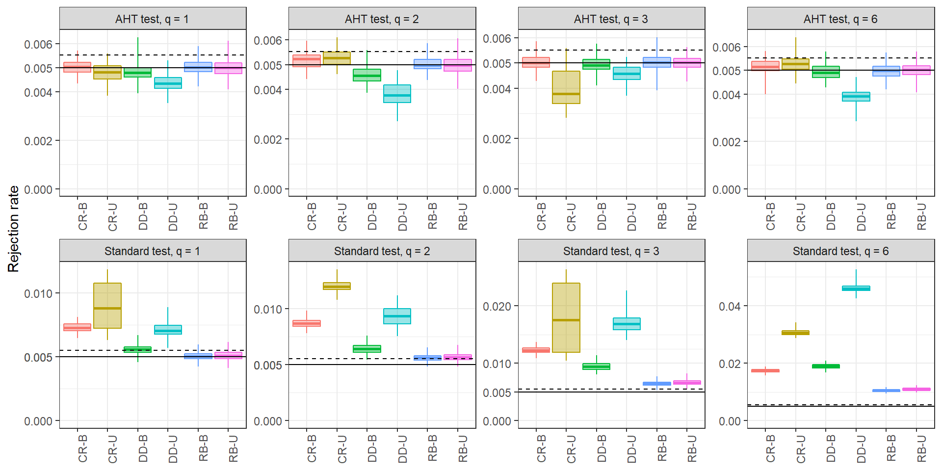
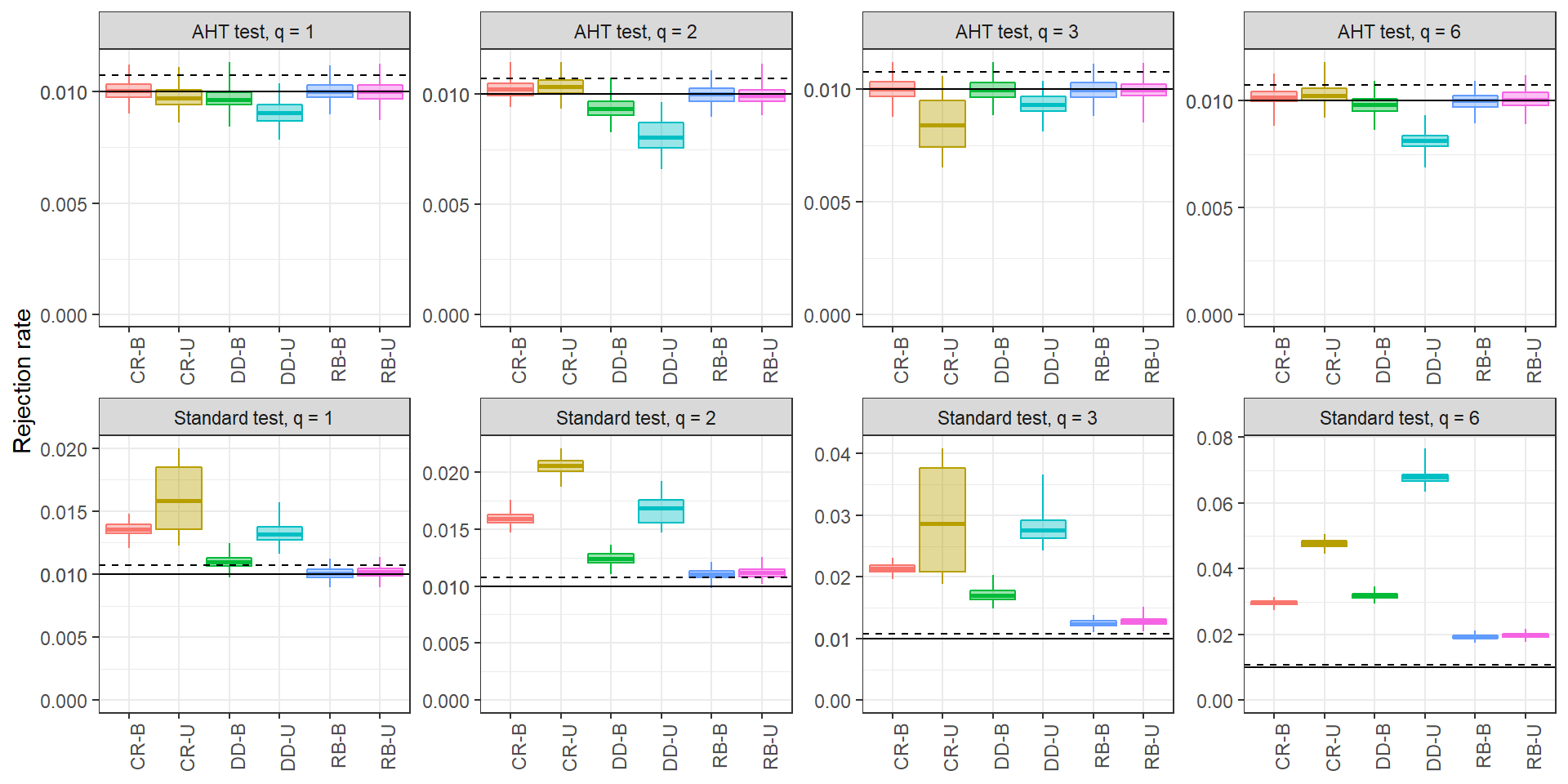
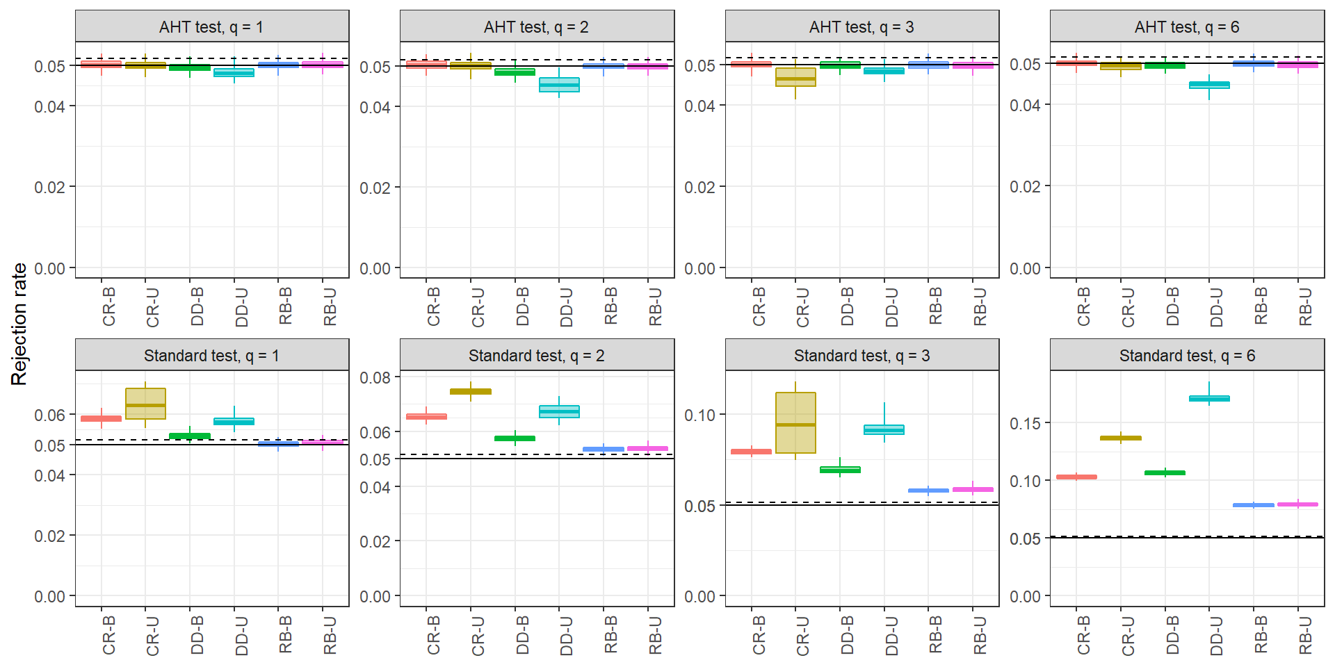
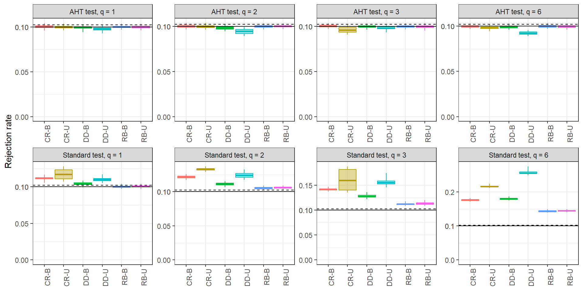
D.3 Rejection rates of AHT test using CR1 or CR2, with and without accounting for absorption

Figure A16: Rejection rates of AHT tests using CR1, CR2, or CR2 calculated without accounting for absorption of fixed effects (CR2*), by sample size ($m$) and dimension of hypothesis ($q$), for $\alpha=.005$.

Figure A17: Rejection rates of AHT tests using CR1, CR2, or CR2 calculated without accounting for absorption of fixed effects (CR2*), by sample size ($m$) and dimension of hypothesis ($q$), for $\alpha=.01$.

Figure A18: Rejection rates of AHT tests using CR1, CR2, or CR2 calculated without accounting for absorption of fixed effects (CR2*), by sample size ($m$) and dimension of hypothesis ($q$), for $\alpha=.05$.

Figure A19: Rejection rates of AHT tests using CR1, CR2, or CR2 calculated without accounting for absorption of fixed effects (CR2*), by sample size ($m$) and dimension of hypothesis ($q$), for $\alpha=.10$.

D.4 Rejection rates of AHT test by degree of working model misspecification

Figure A20: Rejection rates of CR2 AHT test, by treatment effect variance and intra-class correlation for $\alpha=.005$.

Figure A21: Rejection rates of CR2 AHT test, by treatment effect variance and intra-class correlation for $\alpha=.01$.

Figure A22: Rejection rates of CR2 AHT test, by treatment effect variance and intra-class correlation for $\alpha=.05$.

Figure A23: Rejection rates of CR2 AHT test, by treatment effect variance and intra-class correlation for $\alpha=.10$.