Norberg Festschrift

Abstract

Approximations for an unknown density $g$ in terms of a reference density $f_{\nu}$ and its associated orthonormal polynomials are discussed. The main application is the approximation of the density $f$ of a sum $S$ of lognormals which may have different variances or be dependent. In this setting, $g$ may be $f$ itself or a transformed density, in particular that of $\log S$ or an exponentially tilted density. Choices of reference densities $f_{\nu}$ that are considered include normal, gamma and lognormal densities. For the lognormal case, the orthonormal polynomials are found in closed form and it is shown that they are not dense in $L_{2}(f_{\nu})$, a result that is closely related to the lognormal distribution not being determined by its moments and provides a warning to the most obvious choice of taking $f_{\nu}$ as lognormal. Numerical examples are presented and comparison are made to established approaches such as the Fenton–Wilkinson method and skew-normal approximations. Also extension to density estimation for statistical data sets and non-Gaussian copulas are outlined.
Keywords: Lognormal distribution, sums of lognormally distributed random variable, orthogonal polynomial, density estimation, Stieltjes moment problem, numerical approximation of functions, exponential tilting, conditional Monte Carlo, Archimedean copula, Gram–Charlier expansion, Hermite polynomial, Laguerre polynomial

Chapter 1 Orthonormal polynomial expansions
and lognormal sum densities

By Søren Asmussen, Pierre-Olivier Goffard, Patrick J. Laub

1 Introduction

The lognormal distribution arises in a wide variety of disciplines such as engineering, economics, insurance, finance, and across the sciences $\hbox{}{[{\mbox{?}},{\mbox{?}},{\mbox{?}},{\mbox{?}},{\mbox{?}}]}$. Therefore, it is natural that sums $S$ of $n$ lognormals come up in a number of contexts. A basic example in finance is the Black–Scholes model, which assumes that security prices are lognormals, and hence the value of a portfolio with $n$ securities has the form $S$. In insurance, individual claim sizes are often taken as independent lognormals, so the total claim amount in a certain period is again of form $\hbox{}{[{\mbox{?}}]}$. A further example occurs in telecommunications, where the inverse of the signal-to-noise ratio (a measure of performance in wireless systems) can be modeled as a sum of i.i.d. lognormals $\hbox{}{[{\mbox{?}}]}$.

The distribution $S$ is, however, not available in explicit form, and evaluating it numerically or approximating it is considered to be a challenging problem with a long history. The classical approach is to use an approximation with another lognormal distribution. This goes back at least to $\hbox{}{[{\mbox{?}}]}$ and it is nowadays known as the Fenton–Wilkinson method as according to $\hbox{}{[{\mbox{?}}]}$ this approximation was already used by Wilkinson in 1934. However, it can be rather inaccurate when the number of summands is rather small, or when the dispersion parameter is too high. Also tail approximations have been extensively discussed, with the right tail being a classical example in subexponential theory,$\hbox{}{[{\mbox{?}}]}$, and the study of the left tail being more recent, $\hbox{}{[{\mbox{?}}]}$, $\hbox{}{[{\mbox{?}}]}$.

This paper discusses a different method, to approximate the probability density function (p.d.f.) $f$ via polynomials $\{Q_{k}\}$ which are orthonormal w.r.t. some reference measure $\nu$. In the general formulation, one is interested in approximating a target density $g$ using the density $f_{\nu}$ of $\nu$ as reference and $g$ some other density. One then finds a series representation of $g/f_{\nu}$ of the form $\sum_{k=0}^{\infty}a_{k}Q_{k}$, and then the approximation of $g$ is

$$\widehat{g}(x)\ =\ g_{\nu}(x)\sum_{k=0}^{K}a_{k}Q_{k}(x),$$ (1.1)

for some suitable $K$. The most obvious connection to the lognormal sum problem is $g=f$, but we shall look also at other possibilities, to take $g$ as the density of $\log S$ and transform back to get the approximation $\widehat{f}(x)=$ $\widehat{g}(\log x)/x$ or to use an exponential tilting. The choice of $\nu$ is a crucial step, and three candidates for $\nu$ are investigated: the normal, the gamma, and the lognormal distributions.

The form of the $Q_{k}$ is classical for the normal distribution where it is the Hermite polynomials and for the gamma where it is the Laguerre polynomials, but for the lognormal distributions it does not appear to be in the literature and we give here the functional expression (Theorem 1.1). The Fenton–Wilkinson method may be seen as the $K=2$ case of $f_{\nu}$ being lognormal of the general scheme, and this choice of $f_{\nu}$ may be the most obvious one. However, we show that in the lognormal case the orthonormal polynomials are not dense in $L_{2}(f_{\nu})$. This result is closely related to the lognormal distribution not being determined by its moments $\hbox{}{[{\mbox{?}},{\mbox{?}}]}$ and indicates that a lognormal $f_{\nu}$ is potentially dangerous. For this reason, the rest of the paper concentrates on taking the reference distribution as normal (using the logarithmic transformation) or gamma (using exponential tilting).

After discussing the details of the orthonormal polynomials expansions in Sections 2 and 3, we proceed in Section 4 to show a number of numerical examples. The polynomial expansions are compared to existing methods as Fenton–Wilkinson and a more recent approximation in terms of log skew normal distributions $\hbox{}{[{\mbox{?}}]}$, as well as to exact values obtained by numerical quadrature in cases where this is possible or by Monte Carlo density estimation. Section 4 also outlines an extension to statistical data sets and non-Gaussian copulas. Appendices A.1 contains a technical proof and Appendix A.2 some new material on the $\mathcal{SLN}$ Laplace transform.

2 Orthogonal polynomial representation of probability density functions

Let $X$ be a random variable which has a density $f$ with respect to some measure $\lambda\geq 0$ (typically Lebesgue measure on an interval or counting measure on a subset of $\mathbb{Z}$). If $f$ is unknown but the distribution of $X$ is expected to be close to some probability measure $\nu$ with p.d.f. $f_{\nu}$, one may use $f_{\nu}$ as a first approximation to $f$ and next try to improve by invoking suitable correction terms.

In the setting of this paper $X$ is the sum of lognormal r.v.s and the correction terms are obtained by expansions in terms of orthonormal polynomials. Before going into the details of the lognormal example, let us consider the general case.

Assuming all moments of $\nu$ to be finite, the standard Gram–Schmidt orthogonalization technique shows the existence of a set of polynomials $\{Q_{k}\}_{k\in\mathbb{N}_{0}}$ which are orthonormal in $\mathcal{L}^{2}(\nu)$ equipped with the usual inner product $\left<g,h\right>=\int gh\operatorname{d\!}\nu$ and the corresponding norm $\|g\|^{2}=\left<g,g\right>$. That is, the $Q_{k}$ satisfy

$$\left<Q_{i},Q_{j}\right>=\int Q_{i}(x)Q_{j}(x)\operatorname{d\!}\nu(x)=\delta_{ij}\,,\quad i,j\in\mathbb{N}_{0},$$ (2.1)

where $\delta_{ij}$ denotes the Kronecker symbol. If there exists an $\alpha>0$ such that

$$\int\mathrm{e}^{\alpha|x|}\operatorname{d\!}\nu(x)<\infty\,,$$ (2.2)

the set $\{Q_{k}\}_{k\in\mathbb{N}_{0}}$ is complete in $\mathcal{L}^{2}(\nu)$, cf. Chapter $7$ of the book by Nagy $\hbox{}{[{\mbox{?}}]}$. The implication is that if $f/f_{\nu}$ is in $\mathcal{L}^{2}(\nu)$, that is, if

$$\int\frac{f(x)^{2}}{f_{\nu}(x)^{2}}\operatorname{d\!}\nu(x)\ =\ \int\frac{f(x)^{2}}{f_{\nu}(x)}\operatorname{d\!}\lambda(x)\ <\ \infty\,,$$ (2.3)

we may expand $f/f_{\nu}$ as $\sum_{k=0}^{\infty}a_{k}Q_{k}$ where

$$a_{k}\ =\left<f/f_{\nu},Q_{k}\right>\ =\ \int fQ_{k}\,\operatorname{d\!}\lambda\ =\ \mathbb{E}\left[Q_{k}(X)\right]\,.$$ (2.4)

This suggests that we use (1.1) as an approximation of $f$ in situations where the p.d.f. of $X$ is unknown but the moments are accessible.

Remark 1.1

If the first $m$ moments of $X$ and $\nu$ coincide, one has $a_{k}=0$ for $k=1$, …, $m$. When choosing $\nu$, a possible guideline is therefore to match as many moments as possible. $\Diamond$

Due to the Parseval relationship $\sum_{k=0}^{\infty}a_{k}^{2}=\|f/f_{\nu}\|^{2}$, the coefficients of the polynomial expansion, $\{a_{k}\}_{k\in\mathbb{N}_{0}}$, tend toward $0$ as $k\to\infty$. The accuracy of the approximation (1.1), for a given order of truncation $K$, depends upon how swiftly the coefficients decay; note that the $\mathcal{L}^{2}$ loss of the approximation of $f/f_{\nu}$ is $\sum_{K+1}^{\infty}a_{k}^{2}$. Note also that the orthogonal polynomials can be specified recursively (see Thm. 3.2.1 of $\hbox{}{[{\mbox{?}}]}$) which allows a reduction of the computing time required for the coefficients’ evaluation and makes it feasible to consider rather large $K$.

2.1 Normal reference distribution

A common choice as a reference distribution is the normal $\mathcal{N}(\mu,\sigma^{2})$. The associated orthonormal polynomial are given by

$$Q_{k}(x)=\frac{1}{k!2^{k/2}}H_{k}\left(\frac{x-\mu}{\sigma\sqrt{2}}\right),$$ (2.5)

where $\left\{H_{k}\right\}_{k\in\mathbb{N}_{0}}$ are the Hermite polynomials, defined in $\hbox{}{[{\mbox{?}}]}$ for instance. If $f$ is continuous, a sufficient (and close to necessary) condition for $f/f_{\nu}\in\mathcal{L}^{2}(\nu)$ is

$$f(x)\ =\ {\mathcal{O}}\big{(}\mathrm{e}^{-ax^{2}}\big{)}\quad\text{as }x\to\pm\infty\quad\text{with }a>\big{(}4\sigma^{2}\big{)}^{-1}\,.$$ (2.6)

Indeed, we can write the integral in (2.3) as $I_{1}+I_{2}+I_{3}$, the integrals over $(-\infty,-A)$, $[-A,A]$, resp. $(A,\infty)$. Note that $I_{2}<\infty$ follows since the integrand is finite by continuity, whereas the finiteness of $I_{1},I_{3}$ is ensured by the integrands being ${\mathcal{O}}(\mathrm{e}^{-bx^{2}})$ where $b=2a-1/2\sigma^{2}>0$. Similar arguments apply to conditions (2.9) and (2.12) below.

Remark 1.2

The expansion formed by a standard normal baseline distribution and Hermite polynomials is known in the literature as Gram–Charlier expansion of type A, and the application to a standardised sum is the Edgeworth expansion, cf. $\hbox{}{[{\mbox{?}}]}$, $\hbox{}{[{\mbox{?}}]}$. $\Diamond$

2.2 Gamma reference distribution

If $X$ has support $(0,\infty)$, it is natural to look for a $\nu$ with the same property. One of the most apparent possibilities is the gamma distribution, denoted Gamma$(r,m)$ where $r$ is the shape parameter and $m$ the scale parameter. The p.d.f. is

$$f_{\nu}(x)=\frac{x^{r-1}\mathrm{e}^{-x/m}}{m^{r}\Gamma(r)},\hskip 5.69046ptx\in\mathbb{R}_{+}\,.$$ (2.7)

The associated polynomials are given by

$$Q_{n}(x)=(-1)^{n}\left[\frac{\Gamma(n+r)}{\Gamma(n+1)\Gamma(r)}\right]^{-1/2}L_{n}^{r-1}(x/m),\hskip 5.69046ptn\in\mathbb{N}_{0},$$ (2.8)

where $\{L^{r-1}_{n}\}_{n\in\mathbb{N}_{0}}$ denote the generalised Laguerre polynomials, see $\hbox{}{[{\mbox{?}}]}$; in Mathematica these are accessible via the LaguerreL function. Similarly to (2.6), one has the following condition for $f/f_{\nu}\in\mathcal{L}^{2}(\nu)$:

$$\begin{split}f(x)\ &=\ {\mathcal{O}}\big{(}\mathrm{e}^{-\delta x}\big{)}\quad\text{as }x\to\infty\quad\text{with }\delta>1/2m\,,\text{ and }\\ f(x)\ &=\ {\mathcal{O}}\big{(}x^{\beta}\big{)}\quad\text{as }x\to 0\quad\text{with }\beta>r/2-1\,.\end{split}$$ (2.9)

2.3 Lognormal reference distribution

The lognormal distribution $\mathcal{LN}(\mu,\sigma^{2})$ is the distribution of $\mathrm{e}^{Y}$ where $Y\sim\mathcal{N}(\mu,\sigma^{2})$. It has support on $\mathbb{R}_{+}$. The polynomials orthogonal to the $\mathcal{LN}(\mu,\sigma^{2})$ are given in the following proposition, to be proved in the Appendix:

Theorem 1.1

The polynomials orthonormal with respect to the lognormal distribution are given by

$$Q_{k}(x)=\frac{\mathrm{e}^{-\frac{k^{2}\sigma^{2}}{2}}}{\sqrt{\left[\mathrm{e}^{-\sigma^{2}},\mathrm{e}^{-\sigma^{2}}\right]_{k}}}\sum_{i=0}^{k}(-1)^{k+i}\mathrm{e}^{-i\mu-\frac{i^{2}\sigma^{2}}{2}}e_{k-i}\left(1,\ldots,\mathrm{e}^{(k-1)\sigma^{2}}\right)x^{i},$$ (2.10)

for $k\in\mathbb{N}_{0}$ where

$$e_{i}\left(X_{1},\ldots,X_{k}\right)=\begin{cases}\sum_{1\leq j_{1}<\ldots<j_{i}\leq k}X_{j_{1}}\ldots X_{j_{i}},&\mbox{for }i\leq k,\\ 0,&\mbox{for }i>k,\end{cases}$$ (2.11)

are the elementary symmetric polynomials and $\left[x,q\right]_{n}=\prod_{i=0}^{n-1}\left(1-xq^{i}\right)$ is the Q-Pochhammer symbol.

Remark 1.3

The result of Theorem 1.1 does not appear to be in the literature; the closest reference seems to be a 1923 paper by Wigert $\hbox{}{[{\mbox{?}}]}$ who considers the distribution with p.d.f. $\ell\mathrm{e}^{-\ell^{2}\ln^{2}(x)}/\sqrt{\uppi}$ (later called the Stieltjes–Wigert distribution). $\Diamond$

The equivalent of condition (2.6) for $f/f_{\nu}\in\mathcal{L}^{2}(\nu)$ now becomes

$$f(x)\ =\ {\mathcal{O}}\big{(}\mathrm{e}^{-b\log^{2}x}\big{)}\quad\text{for }x\to 0\text{ and }\infty\quad\text{with }b>\big{(}4\sigma^{2}\big{)}^{-1}\,,$$ (2.12)

which is rather mild. However, a key difficulty in taking the reference distribution as lognormal is the following result related to the fact that the lognormal and the Stieltjes-Wigert distributions are not characterised by their moments, see $\hbox{}{[{\mbox{?}},{\mbox{?}},{\mbox{?}},{\mbox{?}}]}$. Hence, the orthogonal polynomials associated with the lognormal p.d.f. and the Stieltjes-Wigert p.d.f. are also the orthogonal polynomials for some other distribution.

Proposition 1.1

The set of orthonormal polynomials in Theorem 1.1 is incomplete in $\mathcal{L}^{2}(\nu)$. That is, span$\{Q_{k}\}_{k\in\mathbb{N}_{0}}$ is a proper subset of $\mathcal{L}^{2}(\nu)$.

Proof 2.2.

Let $Y$ be a r.v. whose distribution is the given lognormal $\nu$ and $X$ a r.v. with a distribution different from $Y$ but with the same moments. According to $\hbox{}{[{\mbox{?}}]}$ such an $X$ can be chosen such that $f_{X}/f_{\nu}$ is bounded and hence in $\mathcal{L}^{2}(\nu)$. The projection of $f/f_{\nu}$ onto ${\rm span}\{Q_{k}\}$ is then

$$\sum_{k=0}^{\infty}\left<f/f_{\nu},Q_{k}\right>Q_{k}\ =\ \sum_{k=0}^{\infty}\mathbb{E}\left[Q_{k}(X)\right]Q_{k}\ =\ \sum_{k=0}^{\infty}\mathbb{E}\left[Q_{k}(Y)\right]Q_{k}$$

$$=\ Q_{0}\ =\ 1\,\neq f/f_{\nu},$$

where the first step used (2.4) and the second that the moments are the same. This implies $f/f_{\nu}\in\mathcal{L}^{2}(\nu)\setminus{\rm span}\{Q_{k}\}$ and the assertion.

2.4 Convergence of the estimators w.r.t. $K$

Orthogonal polynomial approximations generally become more accurate as the order of the approximation $K$ increases. Figure 1 shows a specific orthogonal polynomial approximation, $\widehat{f}_{\mathcal{N}}$ (to be described in Section 3.2), converging to the true $\mathcal{SLN}$ density $f$ for increasing $K$. In this example, we take the $\mathcal{SLN}$ distribution with $\mu=(0,0,0)^{\top}$, $\Sigma_{ii}=0.1$, and $\rho=-0.1$.

Figure 1: Examples of orthogonal polynomial approximations using a $\mathcal{N}(1.13,0.23^{2})$ reference converging to the target $f$ with increasing $K$.

Proposition 1.1 implies that orthogonal polynomial approximations with a lognormal reference distribution cannot be relied upon to converge to the desired target density but may have a different limit (the orthogonal projection described there). The next plot, Figure 2, illustrates this phenomenon. The approximation appears to converge, but not to the target density. Our theoretical discussion suggests that this incorrect limit density has the same moments as the target lognormal distribution, and this was verified numerically for the first few moments,

Figure 2: Example of orthogonal polynomial approximations of $f$ using a $\mathcal{LN}(0,1.22^{2})$ reference not converging to the $\mathcal{LN}(0,1.50^{2})$ target.

Lastly, it must be noted that we cannot in practice take $K$ arbitrarily large, due to numerical errors incurred in calculating the $\{a_{k}\}$ coefficients. Obviously this can be overcome by using infinite precision operations, however this swiftly becomes prohibitively slow. Software tools like Mathematica allow for arbitrarily large but finite precision, which gives on the flexibility to choose a desired accuracy/speed trade-off. We use this technology and select $K\leq 40$.

3 Application to lognormal sums

We now turn to our main case of interest where $X=S$ is a lognormal sum. Specifically,

$$S=\mathrm{e}^{X_{1}}+\ldots+\mathrm{e}^{X_{n}}\,,\quad n\geq 2\,,$$ (3.1)

where the vector $\bm{X}=\left(X_{1},\ldots,X_{n}\right)$ is governed by a multivariate normal distribution $\mathcal{N}\left(\bm{\mu},\bm{\Sigma}\right)$, where $\bm{\mu}=(\mu_{1},\ldots,\mu_{n})^{\top}$ is the mean vector and $\bm{\Sigma}=\left(\sigma_{ij}\right)$ the covariance matrix. We write this distribution as $\mathcal{SLN}\left(\bm{\mu},\bm{\Sigma}\right)$, and hereafter denote its p.d.f. as $f$. We are interested in computing the p.d.f. when the summands exhibit dependency ($\bm{\Sigma}$ is non-diagonal). This is an ambitious goal given that the p.d.f. of the sum of two i.i.d lognormally distributed random variables is already unknown. The validity of the polynomial approximations rely on the $\mathcal{L}^{2}$ integrability condition (2.3), which is difficult to check because the p.d.f. of $S$ is not available. We will need asymptotic results describing the left and the right tail of the distribution of $S$, which we collect in the following subsection.

3.1 Tail asymptotics of lognormal sums

The tail asymptotics of $f(x)$ are given in the following lemma, which simply collects the results from Corollary 2 of $\hbox{}{[{\mbox{?}}]}$ and Theorem 1 of $\hbox{}{[{\mbox{?}}]}$.

Lemma 3.3.

We have

$$f(x) = {\mathcal{O}}(\exp\{-c_{1}\ln(x)^{2}\})\text{ as }x\to 0\text{ and }$$ (3.2)

$$f(x) = {\mathcal{O}}(\exp\{-c_{2}\ln(x)^{2}\})\text{ as }x\to\infty$$ (3.3)

where

$$c_{1}=\big{[}2\min_{\bm{w}\in\Delta}\bm{w}^{\top}\bm{\Sigma}^{-1}\bm{w}\big{]}^{-1}\,\text{ and }\,\,\,c_{2}=\big{[}2\max_{i=1,\dots,n}\sigma_{ii}\big{]}^{-1}\,,$$

with the notation that $\Delta=\{\bm{w}\,|\,w_{i}\in\mathbb{R}_{+},\sum_{i=1}^{n}w_{i}=1\}$.

We are also interested in the asymptotic behaviour of $Z=\ln(S)$ later in the paper. Writing the p.d.f. of $Z$ as $f_{Z}$ we have $f_{Z}(z)=\mathrm{e}^{z}f(\mathrm{e}^{z})$. Together with L’Hôpital’s rule this gives the following results (extending $\hbox{}{[{\mbox{?}}]}$):

Corollary 3.4.

We have

$$f_{Z}(z)\ =\ {\mathcal{O}}(\exp\{-c_{1}z^{2}\})\text{\ as }z\to-\infty\text{ and }$$ (3.4)

$$f_{Z}(z)\ =\ {\mathcal{O}}(\exp\{-c_{2}z^{2}\})\text{\ as }z\to+\infty$$ (3.5)

where the constants are as in Lemma 3.3.

3.2 Lognormal sums via a normal reference distribution

Consider transforming $S$ to $Z=\ln(S)$ and expanding this density with orthogonal polynomials using a normal distribution as reference. That is, our approximation to $f$ using a $\mathcal{N}(\mu,\sigma^{2})$ reference is

$$\widehat{f}_{\mathcal{N}}=\frac{1}{\sigma x}\widehat{f}_{Z}\left(\frac{\ln x-\mu}{\sigma}\right)\quad\text{where}\quad\widehat{f}_{Z}(z)=\phi(z)\sum_{i=1}^{K}a_{i}\,Q_{i}(z)\,,$$

with $\phi(\cdot)$ being the standard normal p.d.f. The following result tells us when the integrability condition $f_{Z}/f_{\nu}\in\mathcal{L}^{2}(\nu)$ is satisfied. It follows immediately by combining (2.6) and Corollary 3.4

Proposition 3.5.

Consider $Z=\ln(S)$ where $S$ is $\mathcal{SLN}(\bm{\mu},\bm{\Sigma})$ distributed. Let $\nu$ be the probability measure associated to the normal distribution $\mathcal{N}(\mu,\sigma^{2})$. We have $f_{Z}/f_{\nu}\in\mathcal{L}^{2}(\nu)$ if

$$2\sigma^{2}>(2c_{2})^{-1}=\max_{i=1,\dots,n}\Sigma_{ii}\,.$$ (3.6)

Computing the $\{\hat{a}_{k}\}_{k\in\mathbb{N}_{0}}$ coefficients can be done using Crude Monte Carlo (CMC), as in

$$\widehat{a}_{k}=\frac{1}{R}\sum_{r=1}^{R}Q_{n}(S_{r})\,,\quad S_{1},\dots,S_{R}\overset{\mathrm{i.i.d.}}{\sim}\mathcal{SLN}(\bm{\mu},\bm{\Sigma})$$

for $k=0,\dots,K$. We can use the same $S_{1}$, …, $S_{R}$ for all $\widehat{a}_{k}$ together with a smoothing technique called common random numbers $\hbox{}{[{\mbox{?}},{\mbox{?}}]}$. Note that a non-trivial amount of computational time is typically spent just constructing the Hermite polynomials. Incorporating the Hermite polynomial’s recurrence relation in our calculations achieved a roughly $40\times$ speed-up compared with using Mathematica’s HermiteH.

3.3 Lognormal sums via a gamma reference distribution

When $\nu$ is Gamma$(r,m)$, it makes little sense to expand $f$ in terms of $\{Q_{k}\}_{k\in\mathbb{N}_{0}}$ and $f_{\nu}$ as the integrability condition (2.9) fails, $f/f_{\nu}\not\in\mathcal{L}^{2}(\nu)$. The workaround consists in using orthogonal polynomials to expand the exponentially tilted distribution, denoted $\mathcal{SLN}_{\theta}(\bm{\mu},\bm{\Sigma})$. This distribution’s p.d.f. is

$$f_{\theta}(x)=\frac{\mathrm{e}^{-\theta x}f(x)}{\mathscr{L}(\theta)}\,,\quad\theta\geq 0,$$ (3.7)

where $\mathscr{L}(\theta)=\mathbb{E}[\mathrm{e}^{-\theta S}]$ is the Laplace transform of $S$. Asmussen et al. $\hbox{}{[{\mbox{?}}]}$ investigated the use of $f_{\theta}(x)$ in approximating the survival function of $S$, and developed asymptotic forms and Monte Carlo estimators of this density.

Remark 3.6.

The use of gamma distribution and Laguerre polynomials links our approach to a well established technique called the Laguerre method. The expansion is an orthogonal projection onto the basis of Laguerre functions constructed by multiplying Laguerre polynomials and the square root of the exponential distribution with parameter $1$. The method is described in $\hbox{}{[{\mbox{?}}]}$. Note also that the damping procedure employed when integrability problems arise is quite similar to considering the exponentially tilted distribution instead of the real one. The use of the gamma distribution as reference is applied to actuarial science in $\hbox{}{[{\mbox{?}},{\mbox{?}}]}$. $\hfill\Diamond$

Using (2.9), we immediately obtain the following result which sheds light on how to tune the parameters of the reference gamma distribution so the integrability condition $f_{\theta}/f_{\nu}\in\mathcal{L}^{2}(\nu)$ is satisfied.

Proposition 3.7.

Consider the r.v. $S_{\theta}$ distributed by the exponentially-tilted $\mathcal{SLN}_{\theta}(\bm{\mu},\bm{\Sigma})$ distribution. Let $\nu$ be the probability measure associated with the Gamma$(r,m)$ distribution. We have $f_{\theta}/f_{\nu}\in\mathcal{L}^{2}(\nu)$ if $m>1/2\theta$.

Hereafter we assume that the parameters $r$ and $m$ of $f_{\nu}\sim\mathrm{Gamma}(r,m)$ are chosen to satisfy Proposition 3.7’s conditions.

Our approximation—based upon rearranging (3.7)—is of the form

$$\widehat{f}(x)=\mathrm{e}^{\theta x}\mathscr{L}(\theta)\widehat{f}_{\theta}(x)=\mathrm{e}^{\theta x}\mathscr{L}(\theta)\sum_{k=0}^{K}a_{k}Q_{k}(x)f_{\nu}(x)\,.$$ (3.8)

The coefficients $a_{k}=\mathbb{E}[Q_{k}(S_{\theta})]$ can be estimated in (at least) three different ways: (i) using CMC, (ii) using Monte Carlo with a change of measure so $\theta\to 0$, or (iii) by directly computing the moments $\mathbb{E}[S_{\theta}^{k}]$. The first method is nontrivial, as simulating from $f_{\theta}$ likely requires using acceptance-rejection (as in $\hbox{}{[{\mbox{?}}]}$). Options (ii) and (iii) use

$$a_{k}=\mathbb{E}[Q_{k}(S_{\theta})]=\mathrel{\mathop{\ordinarycolon}}q_{k0}+q_{k1}\mathbb{E}[S_{\theta}]+\dots+q_{kk}\mathbb{E}[S_{\theta}^{k}]$$ (3.9)

where $\{q_{ki}\}$ are the coefficients in $Q_{k}$, and

$$\mathbb{E}[S_{\theta}^{i}]=\frac{\mathbb{E}[S^{i}\mathrm{e}^{-\theta S}]}{\mathscr{L}(\theta)}=\mathrel{\mathop{\ordinarycolon}}\frac{\mathscr{L}_{i}(\theta)}{\mathscr{L}(\theta)}\,.$$

The $\mathscr{L}_{i}(\theta)$ notation was selected to highlight the link between $\mathbb{E}[S_{n}^{i}\mathrm{e}^{-\theta S_{n}}]$ and the $i$th derivative of $\mathscr{L}(\theta)$.

All three methods require access to the Laplace transform, and method (iii) requires $\mathscr{L}_{i}(\theta)$, however none of $\mathscr{L}(\theta)$ or $\mathscr{L}_{i}(\theta)$ are available in closed form. Our approach to circumvent these problems is presented in the Appendix.

4 Numerical illustrations

We take several approximations $\widehat{f}$ and compare them against the benchmark of numerical integration. One form of $f$ particularly useful for numerical integration, in terms of the $\mathcal{LN}(\bm{\mu},\bm{\Sigma})$ density $f_{\mathcal{LN}}$, is as a surface integral, $f(s)=n^{-\frac{1}{2}}\int_{\Delta_{n}^{s}}f_{\mathcal{LN}}(\bm{x})\operatorname{d\!}\bm{x}$, where $\Delta_{n}^{s}=\{\bm{x}\in\mathbb{R}_{+}^{n}\mathrel{\mathop{\ordinarycolon}}||\bm{x}||_{1}=s\}$. Mathematica integrates this within a reasonable time for $n=2$ to $4$ using NIntegrate and ParametricRegion). For $n>4$ we qualitatively assess the performance of the estimators by plotting them.

The quantitative error measure used is the $\mathcal{L}^{2}$ norm of $(\widehat{f}-f)$ restricted to $(0,\mathbb{E}[S])$. We focus on this region as at one hand it is the hardest to approximate (indeed, Lemma 3.3 shows that just a single lognormal is a theoretically justified approximation of the $\mathcal{SLN}$ right tail) and that at the other of high relevance in applications, see for example the introduction of $\hbox{}{[{\mbox{?}}]}$ and the references therein.

4.1 The estimators

We will compare the following approximations:

• the Fenton-Wilkinson approximation $\widehat{f}_{\mathrm{FW}}$, cf. $\hbox{}{[{\mbox{?}}]}$, consists in approximating the distribution of $S$ by a single lognormal with the same first and second moment;

• the log skew normal approximation $\widehat{f}_{\mathrm{Sk}}$, cf. $\hbox{}{[{\mbox{?}}]}$, is a refinement of Fenton–Wilkinson by using a log skew normal as approximation and fitting the left tail in addition to the first and second moment;

• the conditional Monte Carlo approximation $\widehat{f}_{\mathrm{Cond}}$ , cf. Example 4.3 on p. 146 of $\hbox{}{[{\mbox{?}}]}$, uses the representation $f(x)=$ $\mathbb{E}\bigl{[}\mathbb{P}(S\in\operatorname{d\!}x\,|\,Y)\bigr{]}$ for some suitable $Y$ (here chosen as one of the normal r.v.s $X_{i}$ occurring in (3.1)) and simulates the conditional expectation;

• $\widehat{f}_{\mathcal{N}}$ is the approximation described in Section 3.2 using a logarithmic transformation and the Hermite polynomials with a normal reference distribution;

• $\widehat{f}_{\,\Gamma}$ is the approximation described in Section 3.3 using exponential tilting and the Laguerre polynomials with a gamma reference distribution.

These approximations are all estimators of functions (i.e., not pointwise estimators, such as in $\hbox{}{[{\mbox{?}}]}$) and they do not take excessive computational effort to construct. The first two, $\widehat{f}_{\mathrm{FW}}$ and $\widehat{f}_{\mathrm{Sk}}$, only need $\bm{\mu}$ and $\bm{\Sigma}$ and do not have any Monte Carlo element. Similarly, the estimator $\widehat{f}_{\,\Gamma}$ when utilising the Gauss–Hermite quadrature described in (A.7) in the Appendix does not use Monte Carlo. For the remaining approximations we utilise the common random numbers technique, meaning that the same $R=10^{5}$ i.i.d. $\mathcal{SLN}(\bm{\mu},\bm{\Sigma})$ samples $\bm{S}=(S_{1},\dots,S_{R})^{\top}$ are given to each algorithm. Lastly, all the estimators except $\widehat{f}_{\,\Gamma}$ satisfy $\int\widehat{f}(x)\operatorname{d\!}x=1$. One problem with the orthogonal polynomial estimators is that they can take negative values; this can easily be fixed, but we do not make that adjustment here.

For $\widehat{f}_{\mathcal{N}}$, we take $\mu=\mathbb{E}[Z]$ and $\sigma^{2}=\mathbb{V}\mathrm{ar}[Z]$, calculated using numerical integration. The $\widehat{f}_{\,\Gamma}$ case is more difficult. Equation (3.8) shows that we must impose $\theta m<1$ to ensure that $\widehat{f}_{\,\Gamma}(x)\to 0$ as $x\to\infty$. Exploring different parameter selections showed that fixing $\theta=1$ worked reasonably well. Moment matching $f_{\theta}$ to $f_{\nu}$ leads to the selection of $m$ and $r$. The moments of $f_{\theta}$, $\widehat{\mathbb{E}f_{\theta}}=\widehat{\mathscr{L}}_{1}(\theta)/\widehat{\mathscr{L}}_{0}(\theta)$ and $\widehat{\mathbb{V}\mathrm{ar}f_{\theta}}=\widehat{\mathscr{L}}_{2}(\theta)/\widehat{\mathscr{L}}_{0}(\theta)-\widehat{\mathbb{E}f_{\theta}}^{2}$ can be approximated using the Gauss–Hermite quadrature of (A.7); for this we use $H=64$, 32, 16 for $n=2$, 3, 4 respectively (and CMC for $n>4$).

With these regimes, parameter selection for the reference distributions is automatic, and the only choice the user must make is in selecting $K$. In these tests we examined various $K$ from 1 to 40, and show the best approximations found. The source code for these tests is available online at $\hbox{}{[{\mbox{?}}]}$, and we invite readers to experiment the effect of modifying $K$ and $\theta$ and the parameters of the reference distributions.

4.2 Results

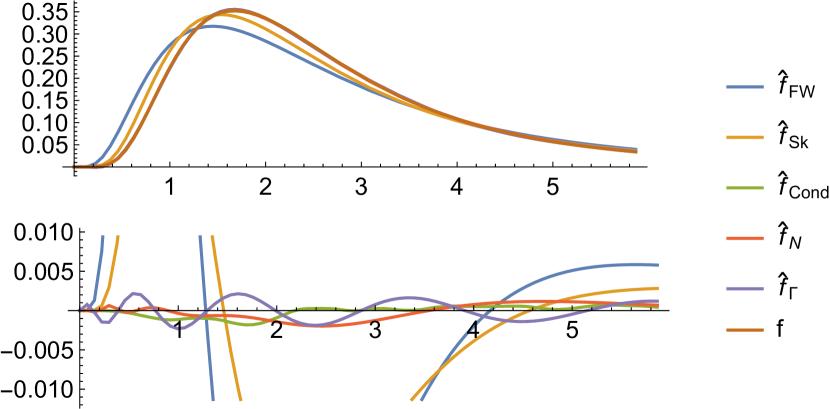
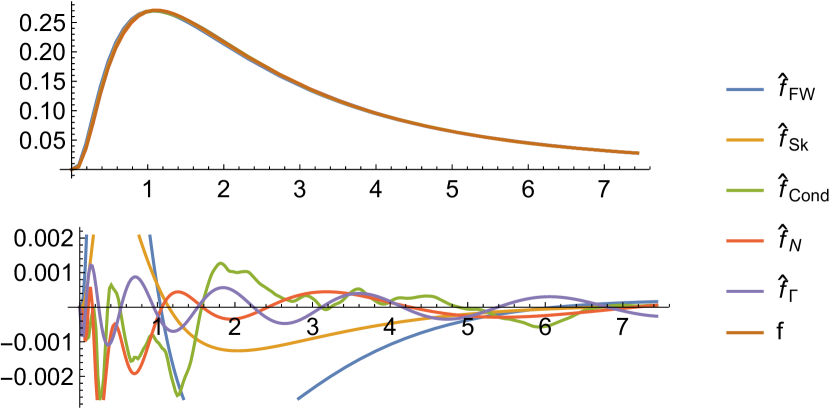
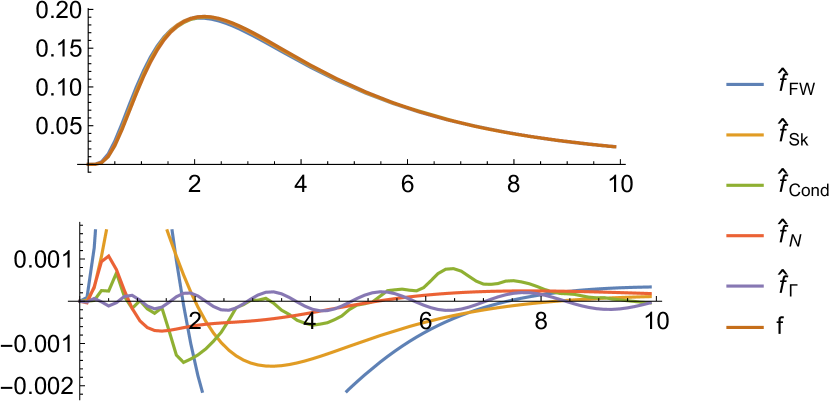
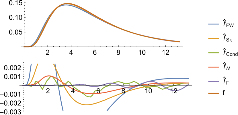
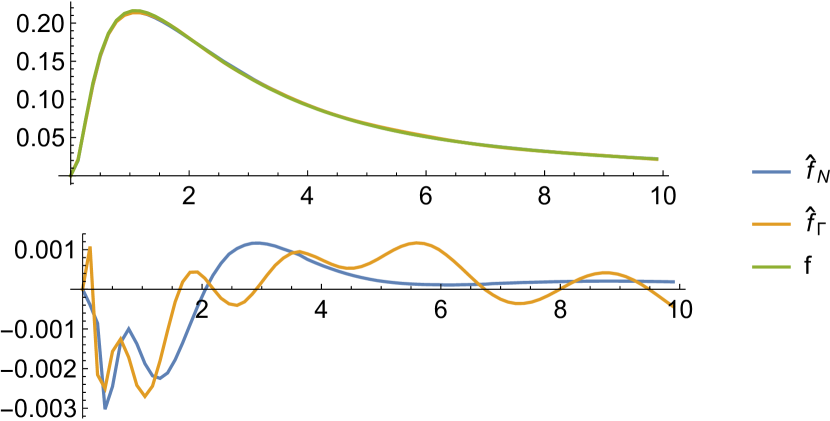
For each test case with $n\leq 4$ we plot the $\widehat{f}(x)$ and $f(x)$ together and then $(\widehat{f}(x)-f(x))$ over $x\in(0,2\mathbb{E}[S])$. A table then shows the $\mathcal{L}^{2}$ errors over $(0,\mathbb{E}[S])$.

	$\widehat{f}_{\mathrm{FW}}$	$\widehat{f}_{\mathrm{Sk}}$	$\widehat{f}_{\mathrm{Cond}}$	$\widehat{f}_{\mathcal{N}}$	$\widehat{f}_{\,\Gamma}$
$\mathcal{L}^{2}$	$8.01{\mkern-2.0mu\times\mkern-2.0mu}10^{-2}$	$4.00{\mkern-2.0mu\times\mkern-2.0mu}10^{-2}$	$1.56{\mkern-2.0mu\times\mkern-2.0mu}10^{-3}$	$1.94{\mkern-2.0mu\times\mkern-2.0mu}10^{-3}$	$2.28{\mkern-2.0mu\times\mkern-2.0mu}10^{-3}$

Test 1: $\bm{\mu}=(0,0)$, $\mathrm{diag}(\bm{\Sigma})=(0.5,1)$, $\rho=-0.2$. Reference distributions used are $\mathcal{N}(0.88,0.71^{2})$ and Gamma($2.43,0.51$) with $K=$ 32, 16 resp.

	$\widehat{f}_{\mathrm{FW}}$	$\widehat{f}_{\mathrm{Sk}}$	$\widehat{f}_{\mathrm{Cond}}$	$\widehat{f}_{\mathcal{N}}$	$\widehat{f}_{\,\Gamma}$
$\mathcal{L}^{2}$	$1.02{\mkern-2.0mu\times\mkern-2.0mu}10^{-2}$	$3.49{\mkern-2.0mu\times\mkern-2.0mu}10^{-3}$	$1.78{\mkern-2.0mu\times\mkern-2.0mu}10^{-3}$	$7.86{\mkern-2.0mu\times\mkern-2.0mu}10^{-4}$	$7.24{\mkern-2.0mu\times\mkern-2.0mu}10^{-4}$

Test 2: $\bm{\mu}=(-0.5,0.5)$, $\mathrm{diag}(\bm{\Sigma})=(1,1)$, $\rho=0.5$. Reference distributions used are $\mathcal{N}(0.91,0.90^{2})$ and Gamma($2.35,0.51$) with $K=$ 32, 16 resp.

	$\widehat{f}_{\mathrm{FW}}$	$\widehat{f}_{\mathrm{Sk}}$	$\widehat{f}_{\mathrm{Cond}}$	$\widehat{f}_{\mathcal{N}}$	$\widehat{f}_{\,\Gamma}$
$\mathcal{L}^{2}$	$9.48{\mkern-2.0mu\times\mkern-2.0mu}10^{-3}$	$3.71{\mkern-2.0mu\times\mkern-2.0mu}10^{-3}$	$1.60{\mkern-2.0mu\times\mkern-2.0mu}10^{-3}$	$1.18{\mkern-2.0mu\times\mkern-2.0mu}10^{-3}$	$3.53{\mkern-2.0mu\times\mkern-2.0mu}10^{-4}$

Test 3: $n=3$, $\mu_{i}=0$, $\Sigma_{ii}=1$, $\rho=0.25$. Reference distributions used are $\mathcal{N}(1.32,0.74^{2})$ and Gamma($3,0.57$) with $K=$ 7, 25 resp.

	$\widehat{f}_{\mathrm{FW}}$	$\widehat{f}_{\mathrm{Sk}}$	$\widehat{f}_{\mathrm{Cond}}$	$\widehat{f}_{\mathcal{N}}$	$\widehat{f}_{\,\Gamma}$
$\mathcal{L}^{2}$	$1.82{\mkern-2.0mu\times\mkern-2.0mu}10^{-2}$	$6.60{\mkern-2.0mu\times\mkern-2.0mu}10^{-3}$	$1.90{\mkern-2.0mu\times\mkern-2.0mu}10^{-3}$	$1.80{\mkern-2.0mu\times\mkern-2.0mu}10^{-3}$	$1.77{\mkern-2.0mu\times\mkern-2.0mu}10^{-4}$

Test 4: $n=4$, $\mu_{i}=0$, $\Sigma_{ii}=1$, $\rho=0.1$. Reference distributions used are $\mathcal{N}(1.32,0.74^{2})$ and Gamma($3.37,0.51$) with $K=$ 18, 18 resp.

The following test case shows the density approximations for a large $n$.

Test 5: Sum of 10 i.i.d. $\mathcal{LN}(0,0.1)$ r.v.s. Reference distributions used are $\mathcal{N}(2.35,0.23^{2})$ and Gamma($12.61,0.25$) with $K=$ 18, 35 resp.

Finally, we fit $\widehat{f}_{\mathcal{N}}$ and $\widehat{f}_{\,\Gamma}$ to simulated data ($10^{5}$ replications) for the sum of lognormals with a non-Gaussian dependence structure. Specifically, we take the sum of $n=3$ standard lognormal r.v.s with a Clayton copula, defined by its distribution function

$$C^{\text{Cl}}_{\theta}(u_{1},\dots,u_{n})=\Big{(}1-n+\sum_{i=1}^{n}u_{i}^{-\theta}\Big{)}^{-1/\theta},\qquad\text{ for }\theta>0\,.$$

The Kendall’s tau correlation of the $C^{\text{Cl}}_{\theta}$ copula is $\tau=\theta/(\theta+2)$ $\hbox{}{[{\mbox{?}}]}$.

Test 6: Sum of 3 $\mathcal{LN}(0,1)$ r.v.s with $C^{\text{Cl}}_{10}(\cdot)$ copula (i.e., $\tau=\frac{5}{6}$). Reference distributions used are $\mathcal{N}(1.46,0.71^{2})$ and Gamma($8.78,0.25$) with $K=40$. The $\mathcal{L}^{2}$ errors of $\widehat{f}_{\mathcal{N}}$ and $\widehat{f}_{\,\Gamma}$ are $2.45\times 10^{-3}$ and $2.04\times 10^{-3}$ respectively.

Our overall conclusion of the numerical examples is that no single method can be considered as universally superior. Of the methods in the literature, the log skew normal approximations is generally better than Fenton-Wilkinson, which is unsurprising given it is an extension introducing one more parameter. The estimators, $\widehat{f}_{\mathcal{N}}$ and $\widehat{f}_{\,\Gamma}$, based on orthogonal polynomial approximation techniques, are very flexible. They also display as least as good and sometimes better p.d.f. estimates over the interval $(0,\mathbb{E}[S])$ and their periodic error indicates that they would supply even more accurate c.d.f. estimates. One should note, however, that their performance relies on the tuning of parameters and that somewhat greater effort is involved in their computation (though this is mitigated through the availability of the software in $\hbox{}{[{\mbox{?}}]}$).

An interesting feature of $\widehat{f}_{\mathcal{N}}$ and $\widehat{f}_{\,\Gamma}$ is that the Frank copula example indicates some robustness to the dependence structure used. In view of the current interest in financial applications of non-Gaussian dependence this seems a promising line for future research.

Acknowledgements

We are grateful to Jakob Schach Møller for helpful discussions on orthonormal expansions.

A.1 Proof of Proposition 1.1

Proof 1..8.

The polynomials orthogonal with respect to the lognormal distribution will be derived using the general formula

$$Q_{n}(x)=\frac{1}{\sqrt{D_{n-1,n-1}D_{n,n}}}\displaystyle\left|\begin{array}[]{cccc}s_{0}&s_{1}&\cdots&s_{n}\\ s_{1}&s_{2}&\cdots&s_{n+1}\\ \vdots&\vdots&&\vdots\\ s_{n-1}&s_{n}&\cdots&s_{2n-1}\\ 1&x&\cdots&x^{n}\end{array}\right|,\hskip 2.84544ptn\geq 1,$$ (A.1)

where $\{s_{n}\}_{n\in\mathbb{N}_{0}}$ denotes the moment sequence of the lognormal distribution and $D_{n,n}=\left|\left\{s_{k,l}\right\}_{0\leq k,l\leq n}\right|$ is a Hankel determinant. The moments of the lognormal distribution are given by $s_{n}=p^{n}q^{n^{2}}$, where $p=\mathrm{e}^{\mu}$ and $q=\mathrm{e}^{\frac{\sigma^{2}}{2}}$. Consider

$$D_{n,n}=\displaystyle\left|\begin{array}[]{cccc}1&pq&\cdots&p^{n}q^{n^{2}}\\ pq&p^{2}q^{4}&&p^{n+1}q^{(n+1)^{2}}\\ \vdots&\vdots&&\vdots\\ p^{n-1}q^{(n-1)^{2}}&p^{n}q^{n^{2}}&\cdots&p^{2n-1}q^{(2n-1)^{2}}\\ p^{n}q^{n^{2}}&p^{n+1}q^{(n+1)^{2}}&\cdots&p^{2n}q^{(2n)^{2}}\end{array}\right|,\hskip 2.84544ptn\geq 1,$$ (A.2)

and denote by $R_{k}$ the $k$th row and by $C_{\ell}$ the $\ell$th column. We apply the elementary operations $R_{k+1}\rightarrow p^{-k}q^{-k^{2}}R_{k+1}$, and $C_{\ell+1}\rightarrow p^{-\ell}q^{-\ell^{2}}C_{\ell+1}$ for $k,\ell=0,\ldots,n$ to get a Vandermonde type determinant. Thus we have

$$D_{n,n}=\mathrm{e}^{n(n+1)\mu}\mathrm{e}^{\frac{n(n+1)(2n+1)}{3}\sigma^{2}}\prod_{k=0}^{n-1}\left[\mathrm{e}^{-\sigma^{2}};\mathrm{e}^{-\sigma^{2}}\right]_{k}\\$$ (A.3)

We expand the determinant in (A.1) with respect to the last row to get

$$Q_{n}(x)=\frac{1}{\sqrt{D_{n-1,n-1}D_{n,n}}}\sum_{k=0}^{n}(-1)^{n+k}x^{k}D_{n-1,n}^{-k},$$ (A.4)

where $D_{n-1,n}^{-k}$ is $D_{n,n}$ with the last row and the $(k+1)$th column deleted. We perform on $D_{n-1,n}^{-k}$ the following operations: $R_{j+1}\rightarrow p^{-j}q^{-j^{2}}R_{j+1}$, for $j=0,\ldots,n-1$, $C_{j+1}\rightarrow p^{-j}q^{-j^{2}}C_{j+1}$, for $j=0,\ldots,k-1$, and finally $C_{j}\rightarrow p^{-j}q^{-j^{2}}C_{j}$, for $j=k+1,\ldots,n$. We obtain

$$D_{n-1,n}^{-k}=p^{n^{2}-k}q^{\frac{2n^{3}+n}{3}-k^{2}}\left|\begin{array}[]{ccccccc}1&\alpha_{0}&\cdots&\alpha_{0}^{k-1}&\alpha_{0}^{k+1}&\cdots&\alpha_{0}^{n}\\ 1&\alpha_{1}&\cdots&\alpha_{1}^{k-1}&\alpha_{1}^{k+1}&\cdots&\alpha_{1}^{n+1}\\ \vdots&\vdots&&\vdots&\vdots&&\vdots\\ 1&\alpha_{n-1}&\cdots&\cdots&\cdots&\cdots&\alpha_{n-1}^{n}\end{array}\right|,$$

where $\alpha_{k}=q^{2k}$, for $k=0,\ldots,n-1$. Expanding the polynomial $B(X)=\prod_{i=0}^{n-1}(x-\alpha_{i})$, we get

$$B(x)=x^{n}+\beta_{n-1}x^{n-1}+\ldots+\beta_{0},$$

where $\beta_{k}=(-1)^{n-k}e_{n-k}\left(\alpha_{0},\ldots,\alpha_{n-1}\right)$, and $e_{k}\left(X_{1},\ldots,X_{n}\right)$ denotes the elementary symmetric polynomial, defined previously in (2.11). We apply the elementary operation $C_{n}\rightarrow C_{n}+\sum_{j=0}^{k-1}a_{j}C_{j+1}+\sum_{j=k+1}^{n-1}a_{j}C_{j}$, followed by $n-k$ cyclic permutations to get

$$D_{n-1,n}^{-k}=p^{n-k}q^{n^{2}-k^{2}}e_{n-k}\left(1,\ldots,q^{2(n-1)}\right)D_{n-1,n-1}.$$ (A.5)

Inserting (A.3) and (A.5) into (A.4) leads to (2.10).

A.2 Computing the coefficients of the expansion $\{a_{k}\}_{k\in\mathbb{N}_{0}}$ in the gamma case

We extend here the techniques developed in $\hbox{}{[{\mbox{?}}]}$ to construct an approximation for $\mathscr{L}_{i}(\theta)$. We note that $\mathscr{L}_{i}(\theta)\propto\int_{\mathbb{R}^{n}}\exp\{-h_{\theta,i}(\bm{x})\}\operatorname{d\!}\bm{x}$ where

$$h_{\theta,i}(\bm{x})=-i\ln(\bm{1}^{\top}\bm{\mathrm{e}}^{\bm{\mu}+\bm{x}})+\theta\bm{1}^{\top}\bm{\mathrm{e}}^{\bm{\mu}+\bm{x}}+\frac{1}{2}\bm{x}^{\top}\bm{\Sigma}^{-1}\bm{x}\,,\quad i\in\mathbb{N}_{0}\,.$$

This uses the notation $\bm{\mathrm{e}}^{\bm{x}}=(\mathrm{e}^{x_{1}},\dots,\mathrm{e}^{x_{n}})^{\top}$. Next, define $\bm{x}^{*}$ as the minimiser of $h_{\theta,i}$ (calculated numerically), and consider a second order Taylor expansion of $h_{\theta,i}$ about $\bm{x}^{*}$. Denote $\widetilde{\mathscr{L}}_{i}(\theta)$ as the approximation where $h_{\theta,i}$ is replaced by this Taylor expansion in $\mathscr{L}_{i}(\theta)$. Simplifying yields

$$\widetilde{\mathscr{L}}_{i}(\theta)=\frac{\exp\{-h_{\theta,i}(\bm{x}^{*})\}}{\sqrt{|\bm{\Sigma}\bm{H}|}}$$ (A.6)

where $\bm{H}$, the Hessian of $h_{\theta,i}$ evaluated at $\bm{x}^{*}$, is

$$\bm{H}=i\frac{\bm{\mathrm{e}}^{\bm{\mu}+\bm{x}^{*}}(\bm{\mathrm{e}}^{\bm{\mu}+\bm{x}^{*}})^{\top}}{(\bm{1}^{\top}\bm{\mathrm{e}}^{\bm{\mu}+\bm{x}^{*}})^{2}}+\bm{\Sigma}^{-1}-\mathrm{diag}(\bm{\Sigma}^{-1}\bm{x}^{*})\,.$$

As $\theta\to\infty$ we have $\widetilde{\mathscr{L}}_{i}(\theta)\to\mathscr{L}_{i}(\theta)$. We can rewrite $\mathscr{L}_{i}(\theta)=\widetilde{\mathscr{L}}_{i}(\theta)I_{i}(\theta)$ and estimate $I_{i}(\theta)$, as in $\hbox{}{[{\mbox{?}}]}$.

Proposition 1..9.

The moments of the exponentially-tilted distribution $\mathcal{SLN}_{\theta}(\bm{\mu},\bm{\Sigma})$, denoted $\mathscr{L}_{i}(\theta)$, can be written as $\mathscr{L}_{i}(\theta)=\widetilde{\mathscr{L}}_{i}(\theta)I_{i}(\theta)$ where $\widetilde{\mathscr{L}}_{i}(\theta)$ is in (A.6) and

$$I_{i}(\theta) =\sqrt{|\bm{\Sigma}\bm{H}|}\,v(\bm{0})^{-1}\,\mathbb{E}[v(\bm{\Sigma}^{\frac{1}{2}}Z)]$$

where $Z\sim\mathcal{N}(\bm{0},\bm{I})$, and

$$v(\bm{z})=\exp\{i\ln(\bm{1}^{\top}\bm{\mathrm{e}}^{\bm{\mu}+\bm{x}^{*}+\bm{z}})-\theta\bm{1}^{\top}\bm{\mathrm{e}}^{\bm{\mu}+\bm{x}^{*}+\bm{z}}-(\bm{x}^{*})^{\top}\bm{\Sigma}^{-1}\bm{z}\}\,.$$

Proof 1..10.

We begin by substituting $\bm{x}=\bm{x}^{*}+\bm{H}^{-\frac{1}{2}}\bm{y}$ into $\mathscr{L}_{i}(\theta)$, then multiply by $\exp\{\pm\text{ some constants}\,\}$:

$$\mathscr{L}_{i}(\theta) =\int_{\mathbb{R}^{n}}\frac{(2\uppi)^{-\frac{n}{2}}}{\sqrt{|\bm{\Sigma}|}}\exp\{i\log(\bm{1}^{\top}\bm{\mathrm{e}}^{\bm{\mu}+\bm{x}})-\theta\bm{1}^{\top}\bm{\mathrm{e}}^{\bm{\mu}+\bm{x}}-\frac{1}{2}\bm{x}^{\top}\bm{\Sigma}^{-1}\bm{x}\}\operatorname{d\!}\bm{x}$$

$$=\int_{\mathbb{R}^{n}}\frac{(2\uppi)^{-\frac{n}{2}}}{\sqrt{|\bm{\Sigma}\bm{H}|}}\exp\{i\log(\bm{1}^{\top}\bm{\mathrm{e}}^{\bm{\mu}+\bm{x}^{*}+\bm{H}^{-\frac{1}{2}}\bm{y}})-\theta\bm{1}^{\top}\bm{\mathrm{e}}^{\bm{\mu}+\bm{x}^{*}+\bm{H}^{-\frac{1}{2}}\bm{y}}$$

$$\qquad-\frac{1}{2}(\bm{x}^{*}+\bm{H}^{-\frac{1}{2}}\bm{y})^{\top}\bm{\Sigma}^{-1}(\bm{x}^{*}+\bm{H}^{-\frac{1}{2}}\bm{y})\}\operatorname{d\!}\bm{y}$$

$$=\widetilde{\mathscr{L}}_{i}(\theta)\exp\{-i\log(\bm{1}^{\top}\bm{\mathrm{e}}^{\bm{\mu}+\bm{x}^{*}})+\theta\bm{1}^{\top}\bm{\mathrm{e}}^{\bm{\mu}+\bm{x}^{*}}\}$$

$$\qquad\times\int_{\mathbb{R}^{n}}(2\uppi)^{-\frac{n}{2}}\exp\{i\log(\bm{1}^{\top}\bm{\mathrm{e}}^{\bm{\mu}+\bm{x}^{*}+\bm{H}^{-\frac{1}{2}}\bm{y}})-\theta\bm{1}^{\top}\bm{\mathrm{e}}^{\bm{\mu}+\bm{x}^{*}+\bm{H}^{-\frac{1}{2}}\bm{y}}$$

$$\qquad\qquad-(\bm{x}^{*})^{\top}\bm{\Sigma}^{-1}\bm{H}^{-\frac{1}{2}}\bm{y}-\frac{1}{2}\bm{y}^{\top}(\bm{\Sigma}\bm{H})^{-1}\bm{y}\}\operatorname{d\!}\bm{y}\,.$$

That is, $\mathscr{L}_{i}(\theta)=\widetilde{\mathscr{L}}_{i}(\theta)I_{i}(\theta)$. In $I_{i}(\theta)$, take the change of variable $\bm{y}=(\bm{\Sigma}\bm{H})^{\frac{1}{2}}\bm{z}$, and the result follows.

Remark 1..11.

The form of $I_{i}(\theta)$ naturally suggests evaluation using Gauss–Hermite quadrature:

$$\widehat{\mathscr{L}}_{i}(\theta)=\frac{\exp\{-h_{\theta,i}(\bm{x}^{*})\}}{v(\bm{0})\,\uppi^{\,n/2}}\sum_{i_{1}=1}^{H}\cdots\sum_{i_{n}=1}^{H}v(\bm{\Sigma}^{\frac{1}{2}}\bm{z})\prod_{j=1}^{n}w_{i_{j}}$$ (A.7)

where $\bm{z}=(z_{i_{1}},\dots,z_{i_{n}})^{\top}$, the set of weights and nodes $\{(w_{i},z_{i})\mathrel{\mathop{\ordinarycolon}}1\leq i\leq H\}$ is specified by the Gauss–Hermite quadrature algorithm, and $H\geq 1$ is the order of the approximation. This approximation is accurate, especially so when the $i$ in $\mathscr{L}_{i}$ becomes large. Even for $\mathscr{L}$ ($=\mathscr{L}_{0}$) this method appears to outperform the quasi-Monte Carlo scheme outlined in $\hbox{}{[{\mbox{?}}]}$. $\hfill\Diamond$

Thus, with $\widehat{\mathscr{L}}_{i}(\theta)$ given in (A.7), we can now estimate the coefficients. The three methods correspond to

1. $\widehat{a}_{k}=R^{-1}\sum_{r=1}^{R}Q_{k}(S_{r})$, for $S_{1}$, …, $S_{R}\overset{\mathrm{i.i.d.}}{\sim}f_{\theta}(x)$,

2. $\widehat{a}_{k}=\sum_{j=0}^{k}q_{kj}\,\widehat{\mathbb{E}[S_{\theta}^{j}]}=q_{k0}+(R\,\widehat{\mathscr{L}}(\theta))^{-1}\sum_{j=1}^{k}q_{kj}\sum_{r=1}^{R}S_{r}^{j}\mathrm{e}^{-\theta S_{r}}$, from (3.9), where $S_{1}$, …, $S_{R}\overset{\mathrm{i.i.d.}}{\sim}f(x)$,

3. $\widehat{a}_{k}=q_{k0}+\widehat{\mathscr{L}}(\theta)^{-1}\sum_{j=1}^{k}q_{kj}\,\widehat{\mathscr{L}}_{j}(\theta)$.

In the numerical illustrations, we switched between using methods (2) and (3) for large and small $n$ respectively. Algorithms for efficient simulation from $f_{\theta}$ is work in progress.

References

• [1] J. Aitchison and J. A. Brown, The Lognormal Distribution with Special Reference to its Uses in Economics. Cambridge University Press (1957).
• [2] E. L. Crow and K. Shimizu, Lognormal Distributions: Theory and Applications. Dekker New York (1988).
• [3] N. L. Johnson, S. Kotz and N. Balakrishnan, Continuous Univariate Distributions, Vol. 1, 2nd edn. New York: Wiley (1994).
• [4] E. Limpert, W. A. Stahel and M. Abbt, Log-normal distributions across the sciences: Keys and clues, BioScience 51, 5, pp. 341–352 (2001).
• [5] D. Dufresne, Sums of lognormals, Tech. rep., Centre for Actuarial Sciences, University of Melbourne (2009).
• [6] O. Thorin and N. Wikstad, Calculation of ruin probabilities when the claim distribution is lognormal, Astin Bulletin 9, 1-2, pp. 231–246 (1977).
• [7] J. A. Gubner, Probability and Random Processes for Electrical and Computer Engineers. Cambridge University Press (2006).
• [8] L. Fenton, The sum of log-normal probability distributions in scatter transmission systems, IRE Transactions on Communications Systems 8, 1, pp. 57–67 (1960).
• [9] N. Marlow, A normal limit theorem for power sums of independent random variables, Bell System Technical Journal 46, 9, pp. 2081–2089 (1967).
• [10] P. Embrechts, C. Klüppelberg and T. Mikosch, Modeling Extremal Events for Insurance and Finance. Springer-Verlag (1997).
• [11] S. Asmussen, J. L. Jensen and L. Rojas-Nandayapa, Exponential family techniques in the lognormal left tail, Scandinavian Journal of Statistics (2015), to appear.
• [12] A. Gulisashvili and P. Tankov, Tail behavior of sums and differences of log-normal random variables, ArXiv preprint arXiv:1309.3057 (2013).
• [13] C. Heyde, On a property of the lognormal distribution, J. Roy. Statist. 5, Ser. B, pp. 392–393 (1963).
• [14] C. Berg, J. P. R. Christensen and P. Ressel, Harmonic Analysis on Semigroups, Graduate Texts in Mathematics, Vol. 100. Springer–Verlag (1984).
• [15] M. B. Hcine and R. Bouallegue, Highly accurate log skew normal approximation to the sum of correlated lognormals, In the Proc. of NeTCoM 2014 (2015).
• [16] B. S. Nagy, Introduction to Real Functions and Orthogonal Expansions. Akadémiai Kiadó (1965).
• [17] G. Szegö, Orthogonal Polynomials, Vol. XXIII. American Mathematical Society Colloquium Publications (1939).
• [18] H. Cramer, Mathematical Methods of Statistics, Vol. 9. Princeton University Press (1999).
• [19] O. E. Barndorff-Nielsen and D. R. Cox, Asymptotic Techniques for use in Statistics. Chapman & Hall (1989).
• [20] S. Wigert, Sur les polynomes orthogonaux et l’approximation des fonctions continues, Almqvist and Wiksell (1923).
• [21] T. S. Chihara, On generalized Stieljes-Wigert and related orthogonal polynomials, Journal of Computational and Applied Mathematics 5, 4, pp. 291–297 (1979).
• [22] J. S. Christiansen, The moment problem associated with the Stieljes-Wigert polynomials, Journal of Mathematical Analysis and Applications 277, 1, pp. 218–245 (2003).
• [23] A. Gulisashvili and P. Tankov, Tail behavior of sums and differences of log-normal random variables, Bernoulli (2015), to appear, accessed online on 26th August 2015 at http://www.e-publications.org/ims/submission/BEJ/user/submissionFile/17119?confirm=ef609013.
• [24] S. Asmussen and L. Rojas-Nandapaya, Asymptotics of sums of lognormal random variables with Gaussian copula, Statistics and Probability Letters 78, 16, pp. 2709–2714 (2008).
• [25] X. Gao, H. Xu and D. Ye, Asymptotic behavior of tail density for sum of correlated lognormal variables, International Journal of Mathematics and Mathematical Sciences (2009).
• [26] S. Asmussen and P. W. Glynn, Stochastic Simulation: Algorithms and Analysis, Stochastic Modelling and Applied Probability series, Vol. 57. Springer (2007).
• [27] P. Glasserman, Monte Carlo Methods in Financial Engineering, Stochastic Modelling and Applied Probability series, Vol. 53. Springer (2003).
• [28] J. Abate, G. Choudhury and W. Whitt, On the Laguerre method for numerically inverting Laplace transforms, INFORMS Journal on Computing 8, 4, pp. 413–427 (1995).
• [29] P.-O. Goffard, S. Loisel and D. Pommeret, A polynomial expansion to approximate the ultimate ruin probability in the compound poisson ruin model, Journal of Computational and Applied Mathematics 296, pp. 499–511 (2016).
• [30] P.-O. Goffard, S. Loisel and D. Pommeret, Polynomial approximations for bivariate aggregate claim amount probability distributions, Methodology and Computing in Applied Probability , pp. 1–24 (2015).
• [31] L. Fenton, The sum of log-normal probability distributions in scatter transmission systems, IRE Transactions on Communications Systems 8, 1, pp. 57–67 (1960).
• [32] P. J. Laub, S. Asmussen, J. L. Jensen and L. Rojas-Nandayapa, Approximating the Laplace transform of the sum of dependent lognormals, Volume 48A of Advances in Applied Probability. (2016), in Festschrift for Nick Bingham, C. M. Goldie and A. Mijatovic (Eds.), Probability, Analysis and Number Theory. To appear.
• [33] S. Asmussen, P.-O. Goffard and P. J. Laub, Online accompaniment for “Orthonormal polynomial expansions and lognormal sum densities” (2016), available at https://github.com/Pat-Laub/SLNOrthogonalPolynomials.
• [34] A. J. McNeil, R. Frey and P. Embrechts, Quantitative Risk Management: Concepts, Techniques and Tools, 2nd edn. Princeton University Press (2015).