Photometric Redshift Estimation for Quasars by Integration of KNN and SVM ^∗

Abstract

The massive photometric data collected from multiple large-scale sky surveys offer significant opportunities for measuring distances of celestial objects by photometric redshifts. However, catastrophic failure is still an unsolved problem for a long time and exists in the current photometric redshift estimation approaches (such as $k$-nearest-neighbor). In this paper, we propose a novel two-stage approach by integration of $k$-nearest-neighbor (KNN) and support vector machine (SVM) methods together. In the first stage, we apply KNN algorithm on photometric data and estimate their corresponding z_phot. By analysis, we find two dense regions with catastrophic failure, one in the range of z${}_{\rm phot}\in[0.3,1.2]$, the other in the range of z${}_{\rm phot}\in[1.2,2.1]$. In the second stage, we map the photometric input pattern of points falling into the two ranges from original attribute space into a high dimensional feature space by Gaussian kernel function in SVM. In the high dimensional feature space, many outlier points resulting from catastrophic failure by simple Euclidean distance computation in KNN can be identified by a classification hyperplane of SVM and further be corrected. Experimental results based on the SDSS (the Sloan Digital Sky Survey) quasar data show that the two-stage fusion approach can significantly mitigate catastrophic failure and improve the estimation accuracy of photometric redshifts of quasars. The percents in different |$\Delta$z| ranges and rms (root mean square) error by the integrated method are $83.47\%$, $89.83\%$, $90.90\%$ and 0.192, respectively, compared to the results by KNN ($71.96\%$, $83.78\%$, $89.73\%$ and 0.204).

1 Introduction

Photometric redshifts are obtained by images or photometry. Compared to spectroscopic redshifts, they show the advantages of high efficiency and low cost. Especially, with the running of multiple ongoing multiband photometric surveys, such as SDSS (the Sloan Digital Sky Survey), UKIDSS (the UKIRT Infrared Deep Sky Survey) and WISE (the Wide-Field Infrared Survey Explorer), a huge volume of photometric data are collected, which are larger than spectroscopic data by two or three orders of magnitude. The massive photometric data offer significant opportunities for measuring distances of celestial objects by photometric redshifts. However, photometric redshifts show the disadvantages of low accuracy compared to spectroscopic redshifts, and require more sophisticated estimation algorithms to overcome the problem. Researchers worldwide have investigated the photometric redshift estimation techniques in recent years. Basically, these techniques are categorized into two types: template-fitting models and data mining approaches. Template-fitting model is the traditional approach for estimating photometric redshifts in astronomy. It extracts features from celestial observational information, such as multiband values, and then matches them with the designed templates constructed by theoretical models or real observations. With feature matching, researchers can estimate photometric redshifts. For example, Bolzonella et al. (2000) estimated photometric redshifts through a standard SED fitting procedure, where SEDs (spectral energy distributions) were obtained from broad-band photometry. Wu et al. (2004) estimated the photometric redshifts of a large sample of quasars with the $\chi^{2}$ minimization technique by using derived theoretical color-redshift relation templates. Rowan-Robinson et al. (2008) proposed an approach using fixed galaxy and quasar templates applied to data at 0.36-4.5 $\mu m$, and on a set of four infrared emission templates fitted to infrared excess data at 3.6-170$\mu m$. Ilbert et al. (2009) applied a template-fitting method (Le Phare) to calculate photometric redshifts in the 2-deg² COSMOS field. Experimental results from the above template-fitting methods showed that their estimation accuracy relied on the templates constructed by either simulation or real observational data.

Data mining approaches apply statistics and machine learning algorithms on a set of training samples and automatically learn complicated functional correlations between multiband photometric observations and their corresponding high confidence redshift parameters. These algorithms are data-driven approaches, rather than template-driven approaches. The experimental results showed that they achieved much accurate photometric estimations in many applications. For example, Ball et al. (2008) applied a nearest neighbor algorithm to estimate photometric redshifts for galaxies and quasars using SDSS and GALEX (the Galaxy Evolution Explorer) data sets. Abdalla et al. (2008) estimated photometric redshifts by using a neural network method. Freeman et al. (2009) proposed a non-linear spectral connectivity analysis for transforming photometric colors to a simpler, more natural coordinate system wherein they applied regression to make redshift estimations. Gerdes et al. (2010) developed a boosted decision tree method, called ArborZ, to estimate photometric redshifts for galaxies. Way et al. (2012) proposed an approach based on Self-Organizing-Mapping (SOM) to estimate photometric redshifts. Bovy et al. (2012) presented the extreme deconvolution technique for simultaneous classification and redshift estimation of quasars and demonstrated that the addition of information from UV and NIR bands was of great importance to photometric quasar-star separation and essentially the redshift degeneracies for quasars were resolved. Carrasco et al. (2013) presented an algorithm using prediction trees and random forest techniques for estimating photometric redshifts, incorporating measurement errors into the calculation while also efficiently dealing with missing values in the photometric data. Brescia et al. (2013) applied the Multi Layer Perceptron with Quasi Newton Algorithm (MLPQNA) to evaluate photometric redshifts of quasars with the data set from four different surveys (SDSS, GALEX, UKIDSS, and WISE).

Though template-fitting approaches and data mining approaches can roughly estimate photometric redshifts, they both suffer the catastrophic failure problem in estimating photometric redshifts of quasars when the spectroscopic redshift is less than 3 (Richards et al. 2001; Weinstein et al. 2004; Wu et al. 2004). Zhang et al. (2013) practically demonstrated that with cross-matched multiband data from multiple surveys, such as SDSS, UKIDSS and WISE, $k$-nearest neighbor (KNN) algorithm can largely solve the catastrophic failure problem and improve photometric redshift estimation accuracy. The method becomes more important as the development of multiple large photometric sky surveys and the coming of the age of astronomical big data. However, during the data preparation process, we need to cross-match multiband information of quasars from multiple photometric surveys. The number of matched quasar records is far less than the original quasar number in a single survey. For example, there are 105,783 quasar samples available in SDSS DR7. However, the number of cross-matched samples from SDSS, WISE and UKIDSS is only 24,089. The cross-matched sample is around one fourth of SDSS quasar data. This shortcoming greatly limits the application scope of this estimation approach to only a small portion of cross-matched quasars observed by all surveys.

In this paper, we propose a novel two-stage photometric redshift estimation approach, i.e., the integration of KNN ($k$-nearest neighbor) and SVM (support vector machine) approaches, to mitigate catastrophic failure for quasars by using relative few band attributes only from a single survey. The paper is organized as follows. Section 2 describes the data used. Section 3 presents a brief overview of KNN, SVM and KNN+SVM. Section 4 gives the experimental results by KNN+SVM. The conclusions and discussions are summarized in Section 5.

2 Data

Our experiments are based on a dataset generated from the Sloan Digital Sky Survey (SDSS; York et al. 2000), which labels highly reliable spectroscopic redshifts and has been widely used in photometric redshift estimation. The dataset was constructed by Zhang et al. (2013) for estimating photometric redshifts of quasars. They used the samples of the Quasar Catalogue V (Schneider et al. 2010) in SDSS DR7, which included 105,783 spectrally confirmed quasars. In each quasar record, five band features $u,g,r,i,z$ are provided. Similar to Zhang et al. (2013), in our experiments, we use these five attributes $u-g,g-r,r-i,i-z,r$ (short for $4C+r$) as the input and the corresponding spectroscopic redshift as a regression output.

3 Methodology

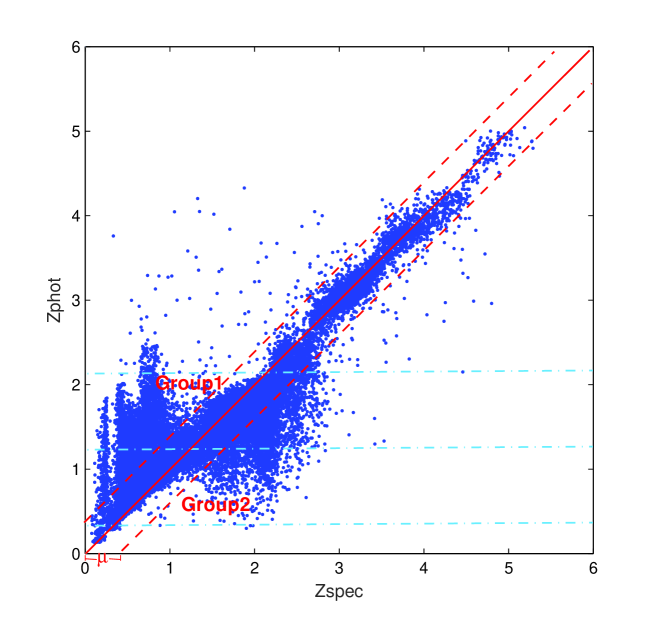
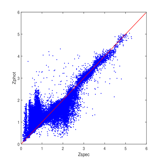
Firstly, we study the characteristics of catastrophic failure for quasars and observe that the outlier points by KNN are clustered into two groups: one group’s spectroscopic redshift z_spec is between 0.2 and 1.1, while its photometric redshift z_phot is between 1.2 and 2.1, and the other group’s z_spec is between 1.4 and 2.3, while its z_phot is between 0.3 and 1.2 (shown in Figure 1). Some points with z_phot falling into Group 1 actually have z_spec close to the range of Group 2, but they are wrongly estimated by KNN and are mixed into Group 1, and vice versa. The two groups look almost 180-degree rotationally symmetric along the 45-degree diagonal line in the z_phot vs. z_spec diagram. The two outlier clusters show that KNN method cannot effectively distinguish outlier points from good estimation points using Euclidean distance in the two regions. Next, we propose a two-stage integration approach by fusion of $k$-nearest neighbors (KNN) and support vector machine (SVM) methods. In the first stage, we apply KNN algorithm on photometric data and estimate their corresponding z_phot. In the second stage, we map photometric multiband input pattern of points falling into the two ranges with z${}_{\rm phot}\in[0.3,1.2]$ and z${}_{\rm phot}\in[1.2,2.1]$ from an original attribute space into a high dimensional feature space by Gaussian kernel function in SVM. In the high dimensional feature space, many outlier points can be identified by a classification hyperplane in SVM and further be corrected. Since most points of catastrophic failure have been identified and corrected, our integration approach can improve the photometric redshift estimation accuracy.

Figure 1: Photometric redshift estimation by KNN estimation. The points in Group 1 and Group 2 are outlier points. $\mu$ is the parameter representing the error tolerant scope. The slant dotted lines give the corrected estimated range of photometric redshifts. The horizontal dotted lines describes the zones of Group 1 and Group 2.

The KNN algorithm generally applies Euclidean distance of attributes (shown in Equation 1) to compute distance between point $m$ and point $n$,

$$d_{m,n}=\sqrt{(f_{m,1}-f_{n,1})^{2}+(f_{m,2}-f_{n,2})^{2}+...+(f_{m,k}-f_{n,k})^{2}}$$ (1)

where $f_{m,j}$($f_{n,j}$) denotes the $j$th attribute among $4C+r$ input pattern for the $m$th ($n$th) points, $k$ represents the total number of attributes. The points in Group 1 and Group 2 show that those outlier quasars cannot be correctly identified in an Euclidean space. In other words, we cannot have a simple plane as a useful separating criterion between points in Group 1 and Group 2. Based on the present data, the provided information is not enough to give good estimation of the outlier points. Now there is a question whether those outlier points can be linearly separable in a high-dimensional non-Euclidean feature space? Thereby, we explore the kernel function in SVM and map features into a high dimension space and test if we can correctly classify outlier points in Group 1 and Group 2. From the analysis above, we propose a two-stage integration approach by fusion of estimation with KNN and classification with SVM.

3.1 Estimation with K-Nearest-Neighbor

K-Nearest-Neighbor (KNN) algorithm is a lazy predictor which requires a training set for learning. It first finds the nearest neighbors by comparing distances between a test sample and training samples that are similar to it in a feature space. Next, it assigns the average value of the nearest neighbors to the test sample as its prediction value. In general, the distance is computed as Euclidean distance described in Equation 1. In the era of big data, we have been collecting more data than ever before and KNN achieves much accurate predictions (Zhang et al. 2013). Thereby, we also use KNN in our research. One disadvantage of KNN is the high computation cost. We apply KD-tree to efficiently implement KNN algorithm.

3.2 Classification with Support Vector Machine

Support Vector Machine (SVM) is an effective classification algorithm based on structural risk minimization principle proposed by Vapnik (1995). Given a training dataset with $n$ records, each record has the pattern of ($x_{i},y_{i}$) for $i=1,2,...,n$, we aim to build a linear classifier with the following Equation 2,

$$f(x)=w\cdot x+b$$ (2)

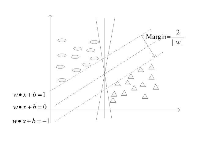
Here, $w$ and $b$ are weight vector and bias respectively. Figure 2 illustrates that several lines can separate two categories of points. In SVM, for minimizing the classification error risk for other test datasets, we aim to find a line (shown as the dash line in Figure 2) with the maximized margin to separate the two classes of points. This principle makes SVM have a better classification accuracy than other competing machine learning models in many classification tasks.

Figure 2: Maximizing classification margin is aimed in SVM. The points on the dotted lines are called as support vectors. The distance between the two dotted lines is named as Margin. When the Margin is maximized, the classification accuracy achieves best.

Figure 3: Linear indistinguishable points in a low dimensional space ($\Re^{d}$) can be separated in a high dimensional space ($\Re^{D}$) by the application of kernel function ($\emptyset$) in SVM. $f(x)=0$ represents the hyperplane that separates the two classes.

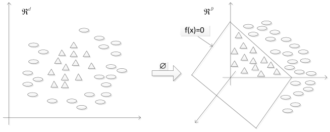
Sometimes, a classification task is hard and not linearly solvable. The left graph in Figure 3 shows one such case. In such case, by Vapnik-Chervonenk in dimension theory, SVM applies a kernel function to promote the original flat space in the ordinary inner product concepts. By the theory of reproducing kernels, we can map the original Euclidean feature space to the high-dimensional non-Euclidean feature space in SVM classification algorithm. Thereby, some of non-linearity problems in the original low-dimensional feature space $\Re^{d}$ become linearly solvable in the high-dimensional space $\Re^{D}$. The right graph in Figure 3 shows a dimension mapping by kernel function to solve the problem. Therefore, Equation 2 can be transformed to the following form by feature mapping function $\emptyset$,

$$f(x)=w\cdot\emptyset(x)+b$$ (3)

In this way, we can have the following objective function and constraints for a SVM classifier as below, and minimize

$$\mid\mid w\mid\mid^{2}+C\sum_{i=1}^{n}\epsilon_{i}$$

subject to

$$y_{i}\cdot(<w,\emptyset(x_{i})>+b)\geq 1-\epsilon_{i}$$ (4)

here, $C$ is a regularization parameter and $\epsilon_{i}$ is a slack variable.

By represented theorem, we have,

$$f(x)=\sum_{i=1}^{n}\alpha_{i}y_{i}\emptyset(x_{i})^{T}\emptyset(x)+b$$ (5)

$\alpha_{i}$ is a parameter with the constraint that $\alpha_{i}\geq 0$. For solving Equation 5, SVM introduces a kernel function defined as,

$$K(x_{i},x)=\emptyset(x_{i})^{T}\emptyset(x)$$ (6)

In this paper, we practically apply Gaussian kernel (shown in Equation 7) to achieve the non-linear classification.

$$K(x_{i},x)=e^{-\frac{\mid\mid x_{1}-x_{2}\mid\mid^{2}}{2\sigma^{2}}}$$ (7)

where $x_{1},x_{2}$ represents vectors of multiband attributes or input patterns observed from a single survey, $\sigma$ is a free parameter.

In this way, we aim to apply a SVM classifier to distinguish the mixture points in Group 1 and other points around the minor diagonal with z${}_{\rm phot}\in[1.2,2.1]$ in the z_phot vs. z_spec diagram. Similarly, we can distinguish points in Group 2 and other points with z${}_{\rm phot}\in[0.3,1.2]$.

3.3 Integration of KNN and SVM for Photometric Redshift Estimation

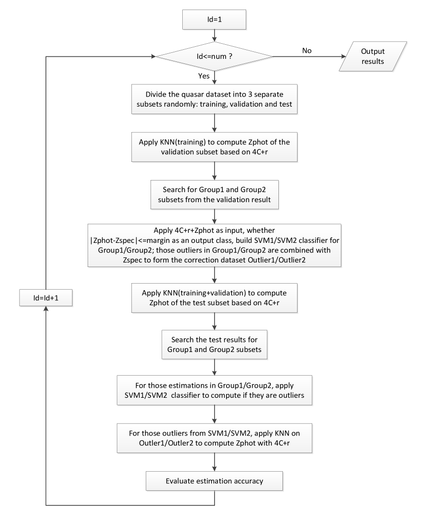
The photometric redshift estimation algorithm by integration of KNN and SVM is presented in the following. To obtain the robust accuracy measure for our integration approach, we repeat the experiments for $num$ rounds. In each round, the data sets will experience the initialization step, KNN step, SVM training step, SVM test step, correction step and evaluation step. In initialization step, we randomly divide the SDSS data set into separate training set, validation set and test set. In KNN step, we apply KNN algorithm ($k=17$) to estimate z_{phot-validation} and z_phot-test based on training set and the union of training set and validation set respectively. In SVM training step, we aim to build two SVM classifiers: SVM1 and SVM2 to distinguish good estimation and outlier points with z${}_{\rm phot-validation}\in[1.2,2.1]$ and z${}_{\rm phot-validation}\in[0.3,1.2]$, respectively. The good estimation or outlier points is defined in the following Equation 8,

$$\left\{\begin{array}[]{rcl}\mid z_{\rm spec}-z_{\rm phot}\mid&\leq&\mu\,\,\,\,\,{\rm good}\\ \mid z_{\rm spec}-z_{\rm phot}\mid&>&\mu\,\,\,\,\,{\rm bad}\end{array}\right.$$ (8)

here, $\mu$ is the parameter which means the error tolerant scope derived from the validation set.

Visually, the good estimation points will fall into area close to 45-degree diagonal line in the diagram, while the outlier points will fall into Group 1 and Group 2 in Figure 1.

Specifically, we use those outlier points with z${}_{\rm phot-validation}\in[1.2,2.1]$ and z${}_{\rm phot-validation}\in[0.3,1.2]$ to construct datasets: Group1_trainingdata and Group2_trainingdata, respectively. In the two datasets, inputs are patterns $4C+r$ and z_phot directly from KNN, and the output is z_spec.

In SVM test step, we apply classifiers SVM1 and SVM2 to identify outlier points.

In correction step, we use KNN algorithm based on Group1_data to compute z_phot for those outlier points distinguished by SVM1 in test data. Since Group1_data and those outlier points have the similar pattern while the output of Group1_trainingdata is z_spec, the KNN algorithm can improve the z_phot estimation. Similarly, we can use Group 2 to train data and then correct outlier points distinguished by SVM2 in test data.

In evaluation step, we apply the percents in different |$\Delta$z| ranges and root mean square (rms) error of $\Delta$z to test our photometric redshift estimation approach. The definition of $\Delta$z is listed in Equation 9.

$$\Delta z=\frac{z_{\rm spec}-z_{\rm phot}}{1+z_{\rm spec}}$$ (9)

The detailed steps of the two-stage method are as following. To be much clearer, the flow chart of the whole process is shown in Figure 4.

LoopId$=1$;

Do while LoopId$\leq num$;

Initialization Step:

Randomly select 1/3 sample from the SDSS quasar sample as the training set, another 1/3 sample as the validation set, and the remaining 1/3 sample as the test set.

KNN Step:

1. Based on training set, we apply KNN ($k=17$) algorithm to estimate z_{phot-validation} for each sample in validation set;

2. Based on the union of training set and validation set, we apply KNN ($k=17$) algorithm to estimate z_phot-test for each sample in test set.

SVM Training Step:

1. For those samples with z${}_{\rm phot-validation}\in[1.2,2.1]$ in validation set, we train a classifier SVM1 with Gaussian kernel, which distinguishes good estimation and outlier points by Equation 8. With those outlier points, we build a data set Group1_trainingdata, which is composed of $4C+r$ and z_phot as the input and z_spec as the output;

2. Similarly, for those samples with z${}_{\rm phot-validation}\in[0.3,1.2]$ in validation set, we train a classifier SVM2 with Gaussian kernel, which distinguishes good estimation and outlier points. With those outlier points, we build a data set Group2_trainingdata, which is composed of $4C+r$ and z_phot as the input and z_spec as the output.

SVM Test Step:

1. For those samples with z${}_{\rm phot-test}\in[1.2,2.1]$ in test set, we apply the classifier SVM1 to distinguish good estimation and outlier points;

2. Similarly, for those samples with z${}_{\rm phot-test}\in[0.3,1.2]$ in test set, we apply the classifier SVM2 to distinguish good estimation and outlier points.

Correction Step:

1. For those outlier points with z${}_{\rm phot-test}\in[1.2,2.1]$ in test set, we apply the KNN algorithm based on the data set Group1_trainingdata;

2. For those outlier points with z${}_{\rm phot-test}\in[0.3,1.2]$ in test set, we apply the KNN algorithm based on the data set Group2_trainingdata.

Evaluation Step:

By comparing z_phot-test and z_spec for all samples in test set, we compute the popular accuracy measures for redshift estimation and rms error of $\Delta$z.

LoopId=LoopId+1;

End do.

Output the mean and standard error for the percents in different |$\Delta$z| ranges and rms error of $\Delta$z to evaluate the accuracy of our proposed integrated approach KNN+SVM.

Figure 4: The flow chart of photometric redshift estimation by the integration of KNN and SVM.

4 Experimental results

In the experiments, we adopt the input pattern $4C+r$ as attributes, which are widely accepted by recent researches on photometric redshift estimation. In our designed algorithm, we practically set $num=10$ and repeat the experiments for 10 times.

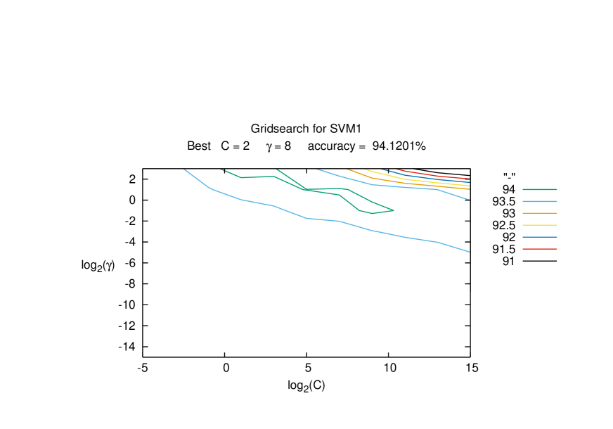
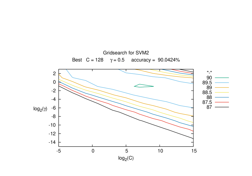
For classification, we apply the widely used tool LIBSVM (Chang, 2011). By using Gaussian kernel function, we train classifiers SVM1 and SVM2 for the sample with z${}_{\rm phot-validation}\in[1.2,2.1]$ and for the sample with z${}_{\rm phot-validation}\in[0.3,1.2]$ in the validation set, separately. To optimize the estimation accuracy, we adjust two parameters controlling the Gaussian kernel in SVM, a cost coefficient $C$ that measures the data unbalance and a factor $\gamma$ depicting the shape of the high dimensional feature space. Other parameters are set to the default values in LIBSVM. In order to obtain the best model parameters, the grid search is adopted. The grid search in SVM1 and SVM2 is indicated in Figure 5. For SVM1, the optimal model parameter $C$ is 2, $\gamma$ is 8, meanwhile, the classification accuracy is 94.12%. For SVM2, the best model parameter $C$ is 128, $\gamma$ is 0.5, the classification accuracy amounts to 90.04%.

Figure 5: Top: the best model parameter in SVM1 is obtained by grid search, i.e. $C$=2, $\gamma$=8, the accuracy of classification achieves 94.12%. Bottom: the best model parameter in SVM2 is obtained by grid search, i.e. $C$=128, $\gamma$=0.5, the accuracy of classification is 90.04%.

With the optimized parameters and the union of the training set and the validation set as a new training set, we compare the estimation accuracy between original KNN ($k=17$) algorithm and our integration approach KNN+SVM. The parameter $\mu$ is a factor to determine whether a point has good estimation or not. We change the value of $\mu$ to check its influence on the estimation accuracy. The results are listed in Table 1. For KNN, the proportions of |$\Delta$z|$<0.1,0.2,0.3$ and rms error of predicted photometric redshifts are 71.96%, 83.78%, 89.73% and 0.204, separately; for KNN+SVM, these optimal measures are 83.47%, 89.83%, 90.90% and 0.192, respectively, when $\mu$=0.3, which are bold in Table 1. Obviously, these criteria for photometric redshift estimation are all significantly improved with the new method. It suggests that the integration approach can effectively correct those outlier points with z${}_{\rm phot}\in[1.2,2.1]$ and z${}_{\rm phot}\in[0.3,1.2]$. Thereby, it can significantly mitigate catastrophic failure and improve the estimation accuracy of photometric redshifts.

Table 1: Comparison of KNN and our integration approach

Method	|$\Delta$z|$<0.1(\%)$	|$\Delta$z|$<0.2(\%)$	|$\Delta$z|$<0.3(\%)$	rms error
KNN($k=17$)	71.96$\pm$0.20	83.78$\pm$0.18	89.73$\pm$0.16	0.204$\pm$0.004
SVM+KNN($\mu=$0.1)	75.06$\pm$3.03	81.43$\pm$2.31	85.51$\pm$1.69	0.232$\pm$0.022
SVM+KNN($\mu=$0.2)	80.86$\pm$1.19	85.56$\pm$1.95	86.57$\pm$1.81	0.224$\pm$0.013
SVM+KNN($\mu=$0.3)	83.47$\pm$0.86	89.83$\pm$0.51	90.90$\pm$0.42	0.192$\pm$0.007
SVM+KNN($\mu=$0.4)	81.63$\pm$0.64	89.53$\pm$0.32	91.54$\pm$0.33	0.193$\pm$0.005
SVM+KNN($\mu=$0.5)	78.89$\pm$0.22	88.30$\pm$0.24	91.63$\pm$0.21	0.194$\pm$0.005
SVM+KNN($\mu=$0.6)	75.84$\pm$0.14	86.60$\pm$0.13	90.58$\pm$0.11	0.199$\pm$0.003

The experimental results also show that without cross-matching multiband observations from multiple surveys, we can effectively apply Gaussian kernel function in SVM to identify outlier points in Group 1 and Group 2 from catastrophic failure by mapping attributes from a single data source into a high dimensional feature space. The identification helps us correct those outlier points and thereby improve estimation accuracy.

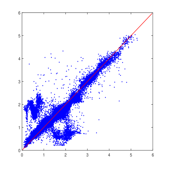
In order to compare the performance of photometric redshift estimation by KNN algorithm with that by KNN and SVM approach, the photometric redshift estimation with these two methods is shown in Figure 6 and Figure 7, respectively. As indicated by Figures 6-7, we can see clearly that the outlier points in both Group 1 and Group 2 have been significantly decreased by adopting the new method KNN+SVM. It intuitively proves that our proposed approach is effective.

Figure 6: Photometric redshift estimation by KNN.

Figure 7: Photometric redshift estimation by KNN+SVM.

5 Conclusions and Discussions

Catastrophic failure is an unsolved problem with a long history existing in most photometric redshift estimation approaches. In this paper, we firstly analyze the reasons of catastrophic failure for quasars and point out that the outlier points result from being non-linearly separable in Euclidean feature space of input pattern. Next, we propose a new estimation approach by integration of KNN and SVM methods together. By Gaussian kernel function in SVM, we map multiband input pattern from an original Euclidean space into a high dimensional feature space. In this way, many outlier points can be identified by a hyperplane and then corrected. The experimental results based on SDSS data for quasars show that the integration approach can significantly mitigate catastrophic failure and improve the photometric redshift estimation accuracy, e.g. the percentages in different |$\Delta$z| ranges and rms error are $83.47\%$, $89.83\%$, $90.90\%$ and 0.192, respectively. While different previous researches of mitigating catastrophic failure by cross-match of data from several surveys, our approach can achieve the similar objective only from a single survey and needn’t cross-match among multiple surveys avoiding cross-match efforts especially for the growing of large survey data. Moreover, not all sources have observation from different surveys. Therefore this method can be widely applied for a single large sky survey photometric data. In addition, the integration method with data from more bands may further improve the accuracy of estimating photometric redshifts of quasars.