Unusual Corrections to the scaling of the entanglement entropy of the excited states in conformal field theory

Lorenzo Cevolani Laboratoire Charles Fabry, Institut d’Optique, CNRS, Univ. Paris-Saclay, 2 avenue Augustin Fresnel, F-91127 Palaiseau cedex, France
Abstract

In this paper we study the scaling of the correction of the Rényi entropy of the excited states in systems described, in the continuum limit, by a conformal field theory (CFT). These corrections scale as L2Δnsuperscript𝐿2Δ𝑛L^{-\frac{2\Delta}{n}}, where L𝐿L is the system size and ΔΔ\Delta is the scaling dimension of a relevant bulk operator located around the singularities of the Riemann surface nsubscript𝑛\mathcal{R}_{n}. Their name is due to their explicit dependence on the Riemann surface nsubscript𝑛\mathcal{R}_{n}. Their presence has been detected in several works on the entanglement entropy in finite size systems, both in the ground and the excited states. Here, we present a general study of these corrections based on the perturbation expansion on nsubscript𝑛\mathcal{R}_{n}. Some of the terms in this expansion are divergent and they will be cured with addition cut-offs. These cut-offs will determine how these corrections scale with the system size L𝐿L. Exact numerical computations of the Rényi entropy of the excited states of the XX model are provided and they confirm our theoretical prediction on the scaling of corrections. They allow also a comparison with the other works present in the literature finding that the corrections, for the excited states, have the exact same form of the ones of the ground state case multiplied by a model dependend function of n𝑛n and l/L𝑙𝐿l/L.

I Introduction

From the birth of the quantum theory, the entanglement has been one of the more fascinating features of the new description of the microscopic world. The presence of a spooky “action at distance” without a classical counterpart, Ref. scrod1 ; scrod2 ; gatto , has raised endless discussions between the fathers of the newborn theory and it has been defined as “the” nature of the quantum mechanics itself, Ref. EPR . After more than a century, entanglement is still a key quantity to understand many phenomena from condensed matter theory to cosmology, Ref. RevModPhys81865 ; Black1 ; Black2 ; Black3 ; algoritmodishor . The Rényi entropy SA(n)=(11n)lnTrρAnsuperscriptsubscript𝑆𝐴𝑛11𝑛Trsuperscriptsubscript𝜌𝐴𝑛S_{A}^{(n)}=\left(\frac{1}{1-n}\right)\ln\text{Tr}\rho_{A}^{n} has been found to be one of the best ways to quantify the amount of entanglement, see Ref. entanglementmagnetic ; RevModPhys80517 , between a system S𝑆S in a pure state and a subsystem A𝐴A described by the reduced density matrix ρAsubscript𝜌𝐴\rho_{A}. The limit n1+𝑛superscript1n\rightarrow 1^{+} gives the Von Neumann entropy SA=TrρAlogρAsubscript𝑆𝐴Trsubscript𝜌𝐴subscript𝜌𝐴S_{A}=-\text{Tr}\rho_{A}\log\rho_{A}. In general, the computation of SA(n)superscriptsubscript𝑆𝐴𝑛S_{A}^{(n)} or SAsubscript𝑆𝐴S_{A} is an impossible task: the complexity of the density matrix of an interacting system does not allow any analytic computations. In the special case of a one dimensional system S𝑆S, whose underlying continuum theory is a CFT, it is possible to compute the Rényi entropy for a generic index n𝑛n. In the case where S𝑆S is in its ground state the Rényi entropy reads

SCFT(n)=c6(1+1n)ln[Lπasin(πlL)]Lc6(1+1n)ln[la]superscriptsubscript𝑆𝐶𝐹𝑇𝑛𝑐611𝑛𝐿𝜋𝑎𝜋𝑙𝐿superscriptsimilar-to𝐿𝑐611𝑛𝑙𝑎S_{CFT}^{(n)}=\frac{c}{6}\left(1+\frac{1}{n}\right)\ln\left[\frac{L}{\pi a}\sin\left(\frac{\pi l}{L}\right)\right]\stackrel{{\scriptstyle L\rightarrow\infty}}{{\sim}}\frac{c}{6}\left(1+\frac{1}{n}\right)\ln\left[\frac{l}{a}\right] (I.1)

where L𝐿L (l𝑙l) is the length of S𝑆S (A𝐴A), a𝑎a is an infrared cut-off and c𝑐c is the central charge of the CFT, Ref. DiFrancesco . This expression has been found in several works, see Ref. Holzey ; Latorre2 ; nontecnica ; PasqualeCFT ; PasqualeEEN ; 351882935 , its universal scaling represents one of the most beautiful consequences of the concept of universality in physics. The previous expression is obtained using a multi-copy system defined by n𝑛n copies of the initial one. These copies are connected one to the other creating a new system that can be seen as defined on a complex Riemann surface nsubscript𝑛\mathcal{R}_{n}, see Ref. CardyDoyon . The same geometrical approach works also if S𝑆S is no longer in its ground state but in one of its excited states, Ref. Berganza ; BerganzaPRL . The difference between the entropy of excited state SΥ(n)superscriptsubscript𝑆Υ𝑛S_{\Upsilon}^{(n)} and the one of the ground state Sgs(n)superscriptsubscript𝑆𝑔𝑠𝑛S_{gs}^{(n)} seen before can be computed again using the multi-copy model on the surface nsubscript𝑛\mathcal{R}_{n}

e(1n)(SΥnSgsn)=limwıj=0n1Υj(w)Υj(w)n[Υ0(w)Υ0(w)1]nsuperscripte1𝑛superscriptsubscript𝑆Υ𝑛superscriptsubscript𝑆𝑔𝑠𝑛subscript𝑤italic-ısubscriptdelimited-⟨⟩superscriptsubscriptproduct𝑗0𝑛1subscriptΥ𝑗𝑤superscriptsubscriptΥ𝑗𝑤subscript𝑛superscriptdelimited-[]subscriptdelimited-⟨⟩subscriptΥ0𝑤superscriptsubscriptΥ0𝑤subscript1𝑛\textit{e}^{(1-n)\left(S_{\Upsilon}^{n}-S_{gs}^{n}\right)}=\lim_{w\rightarrow-\imath\infty}\dfrac{\langle\prod_{j=0}^{n-1}\Upsilon_{j}(w)\Upsilon_{j}^{\dagger}(-w)\rangle_{\mathcal{R}_{n}}}{\left[\langle\Upsilon_{0}(w)\Upsilon_{0}^{\dagger}(-w)\rangle_{\mathcal{R}_{1}}\right]^{n}} (I.2)

where the notation nsubscriptsubscript𝑛\langle\rangle_{\mathcal{R}_{n}} means an expectation value computed over the n𝑛n-sheeted Riemann surface.
The previous expressions have been proved to be true in several systems, both analytically and numerically, see Ref. Latorre2 ; Latorre ; 351882944 ; 351882945 ; 351882956 ; 351882948 ; PhysRevA74022329 ; log1 ; igloi ; log2 ; log3 ; Peschel . Furthermore, some fast oscillating geometry dependent corrections to the continuum CFT results have been found and studied in different systems Ref. steelisa ; massiveunusual ; PhysRevLett104095701 ; EsslerCalabrese ; unusual2 ; unusual3 ; Taddia ; Dalmonte1 ; Dalmonte2 ; Maurizio ; Xavier ; unusual4 . In particular, the scaling of these corrections has been found to be L2Δnsuperscript𝐿2Δ𝑛L^{-\frac{2\Delta}{n}} were ΔΔ\Delta is the scaling dimension of a relevant bulk operator. This behavior is different from the standard renormalization group (RG) flows which is L(Δ2)superscript𝐿Δ2L^{-(\Delta-2)}. The understanding of these corrections is crucial to compare the continuum limit and the numerical data from finite size systems. In Ref. UnusualCorrections it was demonstrated that, for the ground state, these geometry-dependent corrections are due to the presence of a relevant bulk operator Δ>2Δ2\Delta>2 localized around the conical singularities that describe the surface nsubscript𝑛\mathcal{R}_{n}. In this paper we will extend this result to the case of the excited states, where some oscillating corrections to the CFT prediction have been found but not yet studied from the theoretical point of view.
This work is organized as follows: in the first section we will study how Eq. (I.2) is affected by a perturbation to the conformal invariant action. The entanglement entropy can then be evaluated as a power series in the standard perturbation theory on nsubscript𝑛\mathcal{R}_{n}. We will look for divergences in the terms of this expansion and we will cure them with additional cut-offs. This procedure will lead to the scaling behavior of the corrections to the CFT predictions.
In the second part we will present the numerical results. We will study the entanglement entropy of the particle-hole excitations of the XX model, which corresponds to the operator ıϕitalic-ıitalic-ϕ\imath\partial\phi in the continuum limit of this model. We will confirm that the difference between the entropy of this state and the one predicted by the CFT scales as L2nsuperscript𝐿2𝑛L^{-\frac{2}{n}}. We will then compare the corrections in the excited state case with the one found in Ref. correzzioni ; correzzioni2 for the ground state finding that they have the same dependence on the filling. We will conclude that the corrections in the excited states can be written as the ground state ones multiplied by a model dependent function Rn(l/L)subscript𝑅𝑛𝑙𝐿R_{n}(l/L) which was an unknown result before our analysis.

II Unusual corrections

II.1 Perturbation of the function FΥ(n)superscriptsubscript𝐹Υ𝑛F_{\Upsilon}^{(n)}

We will study the unusual corrections to the scaling of the Rényi entropy of the excited states produced by a primary field Υ(w)Υ𝑤\Upsilon(w) defined on nsubscript𝑛\mathcal{R}_{n}. The replica trick approach found for the ground state in Ref. PasqualeCFT can be extended to the excited states taking as "in" state

|Υ=lim(z;z¯)0Υ(z;z¯)|0,ketΥsubscript𝑧¯𝑧0Υ𝑧¯𝑧ket0\ket{\Upsilon}=\lim_{(z;\bar{z})\rightarrow 0}\Upsilon(z;\bar{z})\ket{0}, (II.1)

where |0ket0\ket{0} is the standard vacuum state, and as "out" state

Υ|=lim(z;z¯)0z2hz¯2h¯0|Υ(1z;1z¯).braΥsubscript𝑧¯𝑧0superscript𝑧2superscript¯𝑧2¯bra0Υ1𝑧1¯𝑧\bra{\Upsilon}=\lim_{(z;\bar{z})\rightarrow 0}z^{-2h}\bar{z}^{-2\bar{h}}\bra{0}\Upsilon\left(\frac{1}{z};\frac{1}{\bar{z}}\right). (II.2)

In the previous expressions we used radial quantization, see Ref. DiFrancesco , to define the infinite past and infinite future.
The sub-system A𝐴A is a segment of length l<L𝑙𝐿l<L inside the system S𝑆S and the Riemann surface nsubscript𝑛\mathcal{R}_{n}, defined using the replica trick approach, is mapped onto \mathbb{C} for every value of n𝑛n thanks to the conformal transformation

z=[sin(πwL)sin(π(wl)L)]1n𝑧superscriptdelimited-[]𝜋𝑤𝐿𝜋𝑤𝑙𝐿1𝑛z=\left[\frac{\sin\left(\frac{\pi w}{L}\right)}{\sin\left(\frac{\pi(w-l)}{L}\right)}\right]^{\frac{1}{n}} (II.3)

Calling ρΥnsuperscriptsubscript𝜌Υ𝑛\rho_{\Upsilon}^{n} the density matrix of the excited state and ρInsuperscriptsubscript𝜌𝐼𝑛\rho_{I}^{n} the one of the ground state, following Ref. Berganza ; BerganzaPRL , the Rényi entropy can be written as

FΥn(x)TrρΥnTrρIn=exp((1n)(SΥnSgsn))=limwıj=0n1Υj(w)Υj(w)n[Υ0(w)Υ0(w)1]n,superscriptsubscript𝐹Υ𝑛𝑥𝑇𝑟superscriptsubscript𝜌Υ𝑛𝑇𝑟superscriptsubscript𝜌𝐼𝑛1𝑛superscriptsubscript𝑆Υ𝑛superscriptsubscript𝑆𝑔𝑠𝑛subscript𝑤italic-ısubscriptdelimited-⟨⟩superscriptsubscriptproduct𝑗0𝑛1subscriptΥ𝑗𝑤superscriptsubscriptΥ𝑗𝑤subscript𝑛superscriptdelimited-[]subscriptdelimited-⟨⟩subscriptΥ0𝑤superscriptsubscriptΥ0𝑤subscript1𝑛F_{\Upsilon}^{n}(x)\equiv\dfrac{Tr\rho_{\Upsilon}^{n}}{Tr\rho_{I}^{n}}=\exp\left((1-n)\left(S_{\Upsilon}^{n}-S_{gs}^{n}\right)\right)=\lim_{w\rightarrow-\imath\infty}\dfrac{\langle\prod_{j=0}^{n-1}\Upsilon_{j}(w)\Upsilon_{j}^{\dagger}(-w)\rangle_{\mathcal{R}_{n}}}{\left[\langle\Upsilon_{0}(w)\Upsilon_{0}^{\dagger}(-w)\rangle_{\mathcal{R}_{1}}\right]^{n}}, (II.4)

the limit wı𝑤italic-ıw\rightarrow-\imath\infty fixes the the operators Υ(w)superscriptΥ𝑤\Upsilon^{\dagger}(w) and Υ(w)Υ𝑤\Upsilon(w) to the infinite future and the infinite past. The correlation functions are evaluated using the path integral formulation of quantum mechanics and the conformal invariant action S0subscript𝑆0S_{0}.
Following now Ref. UnusualCorrections we want to study the response of the previous expression to a relevant perturbation Φ(w)Φ𝑤\Phi(w) with scaling dimensions Δ>2Δ2\Delta>2 localized around the conical singularities of the Riemann surface. These conical singularities are identified on nsubscript𝑛\mathcal{R}_{n} by the points w=0𝑤0w=0 and w=l𝑤𝑙w=l and they can be mapped into the complex plane using the mapping II.3. The introduction of this perturbation operator changes the action to

S=S0+λnd2wΦ(w),𝑆subscript𝑆0𝜆subscriptsubscript𝑛superscript𝑑2𝑤Φ𝑤S=S_{0}+\lambda\int_{\mathcal{R}_{n}}d^{2}w\Phi(w), (II.5)

Consequently, II.4 can be formally written as

F~Υn(x)=limwıj=0n1Υj(w)Υj(w)eλnd2wΦ(w)n[Υ0(w)Υ0(w)eλ1d2wΦ(w)1]n,superscriptsubscript~𝐹Υ𝑛𝑥subscript𝑤italic-ısubscriptdelimited-⟨⟩superscriptsubscriptproduct𝑗0𝑛1subscriptΥ𝑗𝑤superscriptsubscriptΥ𝑗𝑤superscripte𝜆subscriptsubscript𝑛superscript𝑑2𝑤Φ𝑤subscript𝑛superscriptdelimited-[]subscriptdelimited-⟨⟩subscriptΥ0𝑤superscriptsubscriptΥ0𝑤superscripte𝜆subscriptsubscript1superscript𝑑2𝑤Φ𝑤subscript1𝑛\tilde{F}_{\Upsilon}^{n}(x)=\lim_{w\rightarrow-\imath\infty}\dfrac{\langle\prod_{j=0}^{n-1}\Upsilon_{j}(w)\Upsilon_{j}^{\dagger}(-w)\textit{e}^{-\lambda\int_{\mathcal{R}_{n}}d^{2}w\,\Phi(w)}\rangle_{\mathcal{R}_{n}}}{\left[\langle\Upsilon_{0}(w)\Upsilon_{0}^{\dagger}(-w)\textit{e}^{-\lambda\int_{\mathcal{R}_{1}}d^{2}w\Phi(w)}\rangle_{\mathcal{R}_{1}}\right]^{n}}, (II.6)

where the correlation functions are here evaluated using the CFT invariant action S0subscript𝑆0S_{0}.
The previous expression can be evaluated as power series of the coupling constant λ1much-less-than𝜆1\lambda\ll 1 which can be written as g/ϵ2Δ𝑔superscriptitalic-ϵ2Δg/\epsilon^{2-\Delta} where g𝑔g is the dimensionless coupling constant, see Ref. DiFrancesco . Taking the logarithm of this expansion we will restrict ourself to the evaluation of just connected Feynman diagrams

ln(F~Υn(x))superscriptsubscript~𝐹Υ𝑛𝑥\displaystyle\ln\left(\tilde{F}_{\Upsilon}^{n}(x)\right) =\displaystyle= ln(FΥn(x))+limit-fromsuperscriptsubscript𝐹Υ𝑛𝑥\displaystyle\ln\left(F_{\Upsilon}^{n}(x)\right)+
+k=1(λ)kk!∫⋯∫njΥj(w)Υj(w)Φ(w1)Φ(w2)Φ(wk)nj=0n1Υj(w)Υj(w)nd2w1d2wksuperscriptsubscript𝑘1superscript𝜆𝑘𝑘subscriptmultiple-integralsubscript𝑛subscriptdelimited-⟨⟩subscriptproduct𝑗subscriptΥ𝑗𝑤superscriptsubscriptΥ𝑗𝑤Φsubscript𝑤1Φsubscript𝑤2Φsubscript𝑤𝑘subscript𝑛subscriptdelimited-⟨⟩superscriptsubscriptproduct𝑗0𝑛1subscriptΥ𝑗𝑤superscriptsubscriptΥ𝑗𝑤subscript𝑛superscript𝑑2subscript𝑤1superscript𝑑2subscript𝑤𝑘\displaystyle+\sum_{k=1}^{\infty}\dfrac{(-\lambda)^{k}}{k!}\idotsint_{\mathcal{R}_{n}}\dfrac{\langle\prod_{j}\Upsilon_{j}(w)\Upsilon_{j}^{\dagger}(-w)\Phi(w_{1})\Phi(w_{2})\dots\Phi(w_{k})\rangle_{\mathcal{R}_{n}}}{\langle\prod_{j=0}^{n-1}\Upsilon_{j}(w)\Upsilon_{j}^{\dagger}(-w)\rangle_{\mathcal{R}_{n}}}d^{2}w_{1}\dots d^{2}w_{k}
n(k=1(λ)kk!∫⋯∫1Υ0(w)Υ0(w)Φ(w1)Φ(w2)Φ(wk)1Υ0(w)Υ0(w)1d2w1d2wk).𝑛superscriptsubscript𝑘1superscript𝜆𝑘𝑘subscriptmultiple-integralsubscript1subscriptdelimited-⟨⟩subscriptΥ0𝑤superscriptsubscriptΥ0𝑤Φsubscript𝑤1Φsubscript𝑤2Φsubscript𝑤𝑘subscript1subscriptdelimited-⟨⟩subscriptΥ0𝑤superscriptsubscriptΥ0𝑤subscript1superscript𝑑2subscript𝑤1superscript𝑑2subscript𝑤𝑘\displaystyle-n\left(\sum_{k=1}^{\infty}\dfrac{(-\lambda)^{k}}{k!}\idotsint_{\mathcal{R}_{1}}\dfrac{\langle\Upsilon_{0}(w)\Upsilon_{0}^{\dagger}(-w)\Phi(w_{1})\Phi(w_{2})\dots\Phi(w_{k})\rangle_{\mathcal{R}_{1}}}{\langle\Upsilon_{0}(w)\Upsilon_{0}^{\dagger}(-w)\rangle_{\mathcal{R}_{1}}}d^{2}w_{1}\dots d^{2}w_{k}\right).

Some terms in the previous expansion have divergences due to the field Φ(w)Φ𝑤\Phi(w), as we will see, and they have to be cured imposing a short distance cut-off ϵitalic-ϵ\epsilon. This corresponds to assume that the continuum theory describes the correct behavior of the correlations just on distances larger than ϵitalic-ϵ\epsilon because for smaller ones the continuum theory does not hold. This approximation is rude but it has been demonstrated to be sufficient to find the correct scaling of the corrections in the ground state case, Ref. UnusualCorrections .
We will study separately the two integrals defining the order λ𝜆\lambda term in Eq. II.1

λnj=0n1Υj(w)Υj(w)Φ(w1)nj=0n1Υj(w)Υj(w)nd2w1λ1Υ0(w)Υ0(w)Φ(w1)1Υ0(w)Υ0(w)1d2w1,𝜆subscriptsubscript𝑛subscriptdelimited-⟨⟩superscriptsubscriptproduct𝑗0𝑛1subscriptΥ𝑗𝑤superscriptsubscriptΥ𝑗𝑤Φsubscript𝑤1subscript𝑛subscriptdelimited-⟨⟩superscriptsubscriptproduct𝑗0𝑛1subscriptΥ𝑗𝑤superscriptsubscriptΥ𝑗𝑤subscript𝑛superscript𝑑2subscript𝑤1𝜆subscriptsubscript1subscriptdelimited-⟨⟩subscriptΥ0𝑤superscriptsubscriptΥ0𝑤Φsubscript𝑤1subscript1subscriptdelimited-⟨⟩subscriptΥ0𝑤superscriptsubscriptΥ0𝑤subscript1superscript𝑑2subscript𝑤1\lambda\int_{\mathcal{R}_{n}}\dfrac{\langle\prod_{j=0}^{n-1}\Upsilon_{j}(w)\Upsilon_{j}^{\dagger}(-w)\Phi(w_{1})\rangle_{\mathcal{R}_{n}}}{\langle\prod_{j=0}^{n-1}\Upsilon_{j}(w)\Upsilon_{j}^{\dagger}(-w)\rangle_{\mathcal{R}_{n}}}d^{2}w_{1}-\lambda\int_{\mathcal{R}_{1}}\dfrac{\langle\Upsilon_{0}(w)\Upsilon_{0}^{\dagger}(-w)\Phi(w_{1})\rangle_{\mathcal{R}_{1}}}{\langle\Upsilon_{0}(w)\Upsilon_{0}^{\dagger}(-w)\rangle_{\mathcal{R}_{1}}}d^{2}w_{1}, (II.8)

and the same for the order λ2superscript𝜆2\lambda^{2}

λ2nj=0n1Υj(w)Υj(w)Φ(w1)Φ(w2)nj=0n1Υj(w)Υj(w)nλ21Υ0(w)Υ0(w)Φ(w1)Φ(w2)1Υ0(w)Υ0(w)1.superscript𝜆2subscriptsubscript𝑛subscriptdelimited-⟨⟩superscriptsubscriptproduct𝑗0𝑛1subscriptΥ𝑗𝑤superscriptsubscriptΥ𝑗𝑤Φsubscript𝑤1Φsubscript𝑤2subscript𝑛subscriptdelimited-⟨⟩superscriptsubscriptproduct𝑗0𝑛1subscriptΥ𝑗𝑤superscriptsubscriptΥ𝑗𝑤subscript𝑛superscript𝜆2subscriptsubscript1subscriptdelimited-⟨⟩subscriptΥ0𝑤superscriptsubscriptΥ0𝑤Φsubscript𝑤1Φsubscript𝑤2subscript1subscriptdelimited-⟨⟩subscriptΥ0𝑤superscriptsubscriptΥ0𝑤subscript1\lambda^{2}\int_{\mathcal{R}_{n}}\dfrac{\langle\prod_{j=0}^{n-1}\Upsilon_{j}(w)\Upsilon_{j}^{\dagger}(-w)\Phi(w_{1})\Phi(w_{2})\rangle_{\mathcal{R}_{n}}}{\langle\prod_{j=0}^{n-1}\Upsilon_{j}(w)\Upsilon_{j}^{\dagger}(-w)\rangle_{\mathcal{R}_{n}}}-\lambda^{2}\int_{\mathcal{R}_{1}}\dfrac{\langle\Upsilon_{0}(w)\Upsilon_{0}^{\dagger}(-w)\Phi(w_{1})\Phi(w_{2})\rangle_{\mathcal{R}_{1}}}{\langle\Upsilon_{0}(w)\Upsilon_{0}^{\dagger}(-w)\rangle_{\mathcal{R}_{1}}}. (II.9)

II.2 The λ𝜆\lambda term on the surface 1subscript1\mathcal{R}_{1}

We start from the order λ𝜆\lambda term defined on the surface 1subscript1\mathcal{R}_{1} which reads

1d2w1limwıΥ0(w)Υ0(w)Φ(w1)1Υ0(w)Υ0(w)1.subscriptsubscript1superscript𝑑2subscript𝑤1subscript𝑤italic-ısubscriptdelimited-⟨⟩subscriptΥ0𝑤superscriptsubscriptΥ0𝑤Φsubscript𝑤1subscript1subscriptdelimited-⟨⟩subscriptΥ0𝑤superscriptsubscriptΥ0𝑤subscript1\int_{\mathcal{R}_{1}}d^{2}w_{1}\lim_{w\rightarrow-\imath\infty}\dfrac{\langle\Upsilon_{0}(w)\Upsilon_{0}^{\dagger}(-w)\Phi(w_{1})\rangle_{\mathcal{R}_{1}}}{\langle\Upsilon_{0}(w)\Upsilon_{0}^{\dagger}(-w)\rangle_{\mathcal{R}_{1}}}. (II.10)

Without loss of generality, we will assume that ΦΦ\Phi is spinless, h¯Φ=hΦsubscript¯ΦsubscriptΦ\bar{h}_{\Phi}=h_{\Phi}, and ΥΥ\Upsilon has just an holomorphic part, hΥ=hsubscriptΥh_{\Upsilon}=h and h¯Υ=0subscript¯Υ0\bar{h}_{\Upsilon}=0. Using the conformal map II.3, the integrand can be mapped from 1subscript1\mathcal{R}_{1} to \mathbb{C} using the standard transformation rule for conformal fields, see Ref. DiFrancesco ,

limwıΥ0(w)Υ0(w)Φ(w1)1Υ0(w)Υ0(w)1=|(Lsin(πx)π)1(eıπxz)(eıπxz)|2hΦΥ(zout)Υ(zin)Φ(z1)Υ(zout)Υ(zin),subscript𝑤italic-ısubscriptdelimited-⟨⟩subscriptΥ0𝑤superscriptsubscriptΥ0𝑤Φsubscript𝑤1subscript1subscriptdelimited-⟨⟩subscriptΥ0𝑤superscriptsubscriptΥ0𝑤subscript1superscript𝐿𝜋𝑥𝜋1superscript𝑒italic-ı𝜋𝑥𝑧superscript𝑒italic-ı𝜋𝑥𝑧2subscriptΦsubscriptdelimited-⟨⟩Υsubscript𝑧𝑜𝑢𝑡superscriptΥsubscript𝑧𝑖𝑛Φsubscript𝑧1subscriptdelimited-⟨⟩Υsubscript𝑧𝑜𝑢𝑡superscriptΥsubscript𝑧𝑖𝑛\lim_{w\rightarrow-\imath\infty}\dfrac{\langle\Upsilon_{0}(w)\Upsilon_{0}^{\dagger}(-w)\Phi(w_{1})\rangle_{\mathcal{R}_{1}}}{\langle\Upsilon_{0}(w)\Upsilon_{0}^{\dagger}(-w)\rangle_{\mathcal{R}_{1}}}=\left|\left(\dfrac{L\sin(\pi x)}{\pi}\right)\dfrac{1}{\left(e^{\imath\pi x}-z\right)\left(e^{-\imath\pi x}-z\right)}\right|^{-2h_{\Phi}}\dfrac{\langle\Upsilon(z_{out})\Upsilon^{\dagger}(z_{in})\Phi(z_{1})\rangle_{\mathbb{C}}}{\langle\Upsilon(z_{out})\Upsilon^{\dagger}(z_{in})\rangle_{\mathbb{C}}}, (II.11)

the points zinsubscript𝑧𝑖𝑛z_{in} and zoutsubscript𝑧𝑜𝑢𝑡z_{out} are the "in" and "out" states mapped on the complex plane from the Riemann surface. The previous expression can be computed explicitly thanks to the conformal invariance on \mathbb{C}

Υ0(z)Υ0(z)Φ(z1)Υ0(z)Υ0(z)=(|2sin(πx)||eıπxz1||eıπxz1|)2hΦ.subscriptdelimited-⟨⟩subscriptΥ0superscript𝑧superscriptsubscriptΥ0𝑧Φsubscript𝑧1subscriptdelimited-⟨⟩subscriptΥ0superscript𝑧superscriptsubscriptΥ0𝑧superscript2𝜋𝑥superscript𝑒italic-ı𝜋𝑥subscript𝑧1superscript𝑒italic-ı𝜋𝑥subscript𝑧12subscriptΦ\dfrac{\langle\Upsilon_{0}(z^{\prime})\Upsilon_{0}^{\dagger}(z)\Phi(z_{1})\rangle_{\mathbb{C}}}{\langle\Upsilon_{0}(z^{\prime})\Upsilon_{0}^{\dagger}(z)\rangle_{\mathbb{C}}}=\left(\dfrac{\left|2\sin(\pi x)\right|}{\left|e^{\imath\pi x}-z_{1}\right|\left|e^{-\imath\pi x}-z_{1}\right|}\right)^{2h_{\Phi}}. (II.12)

Even if this expression depends on the variable z1subscript𝑧1z_{1} on the complex plane, its dependence is canceled out by the transformation factor from nsubscript𝑛\mathcal{R}_{n} to \mathbb{C}. The integrand of II.10 is then a constant and it has no divergences around the conical singularities

limwıΥ0(w)Υ0(w)Φ(w1)1Υ0(w)Υ0(w)1=(2πL)2hΦ.subscript𝑤italic-ısubscriptdelimited-⟨⟩subscriptΥ0𝑤superscriptsubscriptΥ0𝑤Φsubscript𝑤1subscript1subscriptdelimited-⟨⟩subscriptΥ0𝑤superscriptsubscriptΥ0𝑤subscript1superscript2𝜋𝐿2subscriptΦ\lim_{w\rightarrow-\imath\infty}\dfrac{\langle\Upsilon_{0}(w)\Upsilon_{0}^{\dagger}(-w)\Phi(w_{1})\rangle_{\mathcal{R}_{1}}}{\langle\Upsilon_{0}(w)\Upsilon_{0}^{\dagger}(-w)\rangle_{\mathcal{R}_{1}}}=\left(\dfrac{2\pi}{L}\right)^{2h_{\Phi}}. (II.13)

No further cut-off of order ϵitalic-ϵ\epsilon is needed and the scaling of this term is given by the coupling constant λ=g/ϵ2Δ𝜆𝑔superscriptitalic-ϵ2Δ\lambda=g/\epsilon^{2-\Delta}.

II.3 The λ2superscript𝜆2\lambda^{2} term on the surface 1subscript1\mathcal{R}_{1}

On the same Riemann surface 1subscript1\mathcal{R}_{1} we can study the next order λ2superscript𝜆2\lambda^{2} of II.1 which reads

1𝑑w1𝑑w2limwıΥ(w)Υ(w)Φ(w1)Φ(w2)1Υ(w)Υ(w)1,subscriptdouble-integralsubscript1differential-dsubscript𝑤1differential-dsubscript𝑤2subscript𝑤italic-ısubscriptdelimited-⟨⟩Υsuperscript𝑤superscriptΥ𝑤Φsubscript𝑤1Φsubscript𝑤2subscript1subscriptdelimited-⟨⟩Υsuperscript𝑤superscriptΥ𝑤subscript1\iint_{\mathcal{R}_{1}}dw_{1}dw_{2}\lim_{w\rightarrow-\imath\infty}\dfrac{\langle\Upsilon(w^{\prime})\Upsilon^{\dagger}(w)\Phi(w_{1})\Phi(w_{2})\rangle_{\mathcal{R}_{1}}}{\langle\Upsilon(w^{\prime})\Upsilon^{\dagger}(w)\rangle_{\mathcal{R}_{1}}}, (II.14)

as usual the integrand can be mapped from this Riemann surface to \mathbb{C} thanks to conformal symmetry

Υ(w)Υ(w)Φ(w1)Φ(w2)1Υ(w)Υ(w)1=|dw1dz1|2hΦ|dw2dz2|2hΦΥ(z0)Υ(z0)Φ(z1)Φ(z2)Υ(z0)Υ(z0),subscriptdelimited-⟨⟩Υsuperscript𝑤superscriptΥ𝑤Φsubscript𝑤1Φsubscript𝑤2subscript1subscriptdelimited-⟨⟩Υsuperscript𝑤superscriptΥ𝑤subscript1superscript𝑑subscript𝑤1𝑑subscript𝑧12subscriptΦsuperscript𝑑subscript𝑤2𝑑subscript𝑧22subscriptΦsubscriptdelimited-⟨⟩Υsuperscriptsubscript𝑧0superscriptΥsubscript𝑧0Φsubscript𝑧1Φsubscript𝑧2subscriptdelimited-⟨⟩Υsuperscriptsubscript𝑧0superscriptΥsubscript𝑧0\dfrac{\langle\Upsilon(w^{\prime})\Upsilon^{\dagger}(w)\Phi(w_{1})\Phi(w_{2})\rangle_{\mathcal{R}_{1}}}{\langle\Upsilon(w^{\prime})\Upsilon^{\dagger}(w)\rangle_{\mathcal{R}_{1}}}=\left|\dfrac{dw_{1}}{dz_{1}}\right|^{-2h_{\Phi}}\left|\dfrac{dw_{2}}{dz_{2}}\right|^{-2h_{\Phi}}\dfrac{\langle\Upsilon(z_{0}^{\prime})\Upsilon^{\dagger}(z_{0})\Phi(z_{1})\Phi(z_{2})\rangle_{\mathbb{C}}}{\langle\Upsilon(z_{0}^{\prime})\Upsilon^{\dagger}(z_{0})\rangle_{\mathbb{C}}}, (II.15)

but in this case, the conformal invariance is not sufficient to fix completely the four point function on the complex plane

Υ0(w)Υ0(w)Φ(w1)Φ(w2)1Υ0(w)Υ0(w)1=|dw1dz1|2hΦ|dw2dz2|2hΦ|z1z2|4hΦF(η;η¯).subscriptdelimited-⟨⟩subscriptΥ0superscript𝑤superscriptsubscriptΥ0𝑤Φsubscript𝑤1Φsubscript𝑤2subscript1subscriptdelimited-⟨⟩subscriptΥ0superscript𝑤superscriptsubscriptΥ0𝑤subscript1superscript𝑑subscript𝑤1𝑑subscript𝑧12subscriptΦsuperscript𝑑subscript𝑤2𝑑subscript𝑧22subscriptΦsuperscriptsubscript𝑧1subscript𝑧24subscriptΦ𝐹𝜂¯𝜂\dfrac{\langle\Upsilon_{0}(w^{\prime})\Upsilon_{0}^{\dagger}(w)\Phi(w_{1})\Phi(w_{2})\rangle_{\mathcal{R}_{1}}}{\langle\Upsilon_{0}(w^{\prime})\Upsilon_{0}^{\dagger}(w)\rangle_{\mathcal{R}_{1}}}=\left|\dfrac{dw_{1}}{dz_{1}}\right|^{-2h_{\Phi}}\left|\dfrac{dw_{2}}{dz_{2}}\right|^{-2h_{\Phi}}|z_{1}-z_{2}|^{-4h_{\Phi}}F\left(\eta;\bar{\eta}\right). (II.16)

where F(η;η¯)𝐹𝜂¯𝜂F(\eta;\bar{\eta}) is an invariant continuous scalar function of the anharmonic ratio

η=(z0z1)(z0z2)(z0z2)(z0z1).𝜂superscriptsubscript𝑧0subscript𝑧1subscript𝑧0subscript𝑧2superscriptsubscript𝑧0subscript𝑧2subscript𝑧0subscript𝑧1\eta=\dfrac{(z_{0}^{\prime}-z_{1})(z_{0}-z_{2})}{(z_{0}^{\prime}-z_{2})(z_{0}-z_{1})}. (II.17)

Eq. II.16 exhibits the same dependence on the variables z1subscript𝑧1z_{1} and z2subscript𝑧2z_{2} as the correlator Φ(w1)Φ(w2)delimited-⟨⟩Φsubscript𝑤1Φsubscript𝑤2\langle\Phi(w_{1})\Phi(w_{2})\rangle in the ground state case Ref. UnusualCorrections , but here it is multiplied by an invariant continuous function of η𝜂\eta. In the limit where z1subscript𝑧1z_{1} and z2subscript𝑧2z_{2} approach together the conical singularities on \mathbb{C}, the function F(η;η¯)𝐹𝜂¯𝜂F(\eta;\bar{\eta}) tends to a constant thanks to its continuity, see Ref. DiFrancesco . Its contribution to Eq. II.14 is an overall constant factor which can be ignored in the followings.
We can then study the integral II.16 using the explicit expression found for the integrand and the fact that F(η:η¯)F\left(\eta:\bar{\eta}\right) is a approximatively constant in this region

F(η;η¯)2λ2𝑑z1𝑑z2|dw1dz1|2hΦ|dw2dz2|2hΦ|z1z2|4hΦ.𝐹𝜂¯𝜂2superscript𝜆2subscriptdifferential-dsubscript𝑧1subscriptdifferential-dsubscript𝑧2superscript𝑑subscript𝑤1𝑑subscript𝑧12subscriptΦsuperscript𝑑subscript𝑤2𝑑subscript𝑧22subscriptΦsuperscriptsubscript𝑧1subscript𝑧24subscriptΦ\frac{F\left(\eta;\bar{\eta}\right)}{2}\lambda^{2}\int_{\mathbb{C}}dz_{1}\int_{\mathbb{C}}dz_{2}\left|\dfrac{dw_{1}}{dz_{1}}\right|^{-2h_{\Phi}}\left|\dfrac{dw_{2}}{dz_{2}}\right|^{-2h_{\Phi}}|z_{1}-z_{2}|^{-4h_{\Phi}}. (II.18)

The contribution from the region z10similar-tosubscript𝑧10z_{1}\sim 0 and z2subscript𝑧2z_{2}\rightarrow\infty can be easily computed because the integrand factorizes and we can evaluate separately the two contributions from the two conical singularities. For the region z10similar-tosubscript𝑧10z_{1}\sim 0

d2z1|dw1dz1|22hΦ1d2w1|πLsin(πx)|2hΦ=2π|Lsin(πx)π|2hΦϵ2.subscriptsuperscript𝑑2subscript𝑧1superscript𝑑subscript𝑤1𝑑subscript𝑧122subscriptΦsubscriptsubscript1superscript𝑑2subscript𝑤1superscript𝜋𝐿𝜋𝑥2subscriptΦ2𝜋superscript𝐿𝜋𝑥𝜋2subscriptΦsuperscriptitalic-ϵ2\int_{\mathbb{C}}d^{2}z_{1}\left|\dfrac{dw_{1}}{dz_{1}}\right|^{2-2h_{\Phi}}\approx\int_{\mathcal{R}_{1}}d^{2}w_{1}\left|\dfrac{\pi}{L\sin(\pi x)}\right|^{2h_{\Phi}}=2\pi\left|\dfrac{L\sin(\pi x)}{\pi}\right|^{-2h_{\Phi}}\epsilon^{2}. (II.19)

where the prefactor comes out from the linearization of II.3 around the conical singularity w=0𝑤0w=0. This integral is divergent and we need to impose a cut-off of order ϵitalic-ϵ\epsilon. The same procedure has to be done for the integral on z2subscript𝑧2z_{2} approximated around wl𝑤𝑙w\approx l

d2z2|dw2dz2|2|dz2dw2|2hΦ|z2|4hΦ=|Lsin(πx)π|2hΦ1d2w2=2π|Lsin(πx)π|2hΦϵ2.subscriptsuperscript𝑑2subscript𝑧2superscript𝑑subscript𝑤2𝑑subscript𝑧22superscript𝑑subscript𝑧2𝑑subscript𝑤22subscriptΦsuperscriptsubscript𝑧24subscriptΦsuperscript𝐿𝜋𝑥𝜋2subscriptΦsubscriptsubscript1superscript𝑑2subscript𝑤22𝜋superscript𝐿𝜋𝑥𝜋2subscriptΦsuperscriptitalic-ϵ2\int_{\mathbb{C}}d^{2}z_{2}\left|\dfrac{dw_{2}}{dz_{2}}\right|^{2}\left|\dfrac{dz_{2}}{dw_{2}}\right|^{2h_{\Phi}}\left|z_{2}\right|^{-4h_{\Phi}}=\left|\dfrac{L\sin(\pi x)}{\pi}\right|^{-2h_{\Phi}}\int_{\mathcal{R}_{1}}d^{2}w_{2}=2\pi\left|\dfrac{L\sin(\pi x)}{\pi}\right|^{-2h_{\Phi}}\epsilon^{2}. (II.20)

This expression needs to be further regulated imposing a cut-off of order 1/ϵ1italic-ϵ1/\epsilon on the upper bound. Taking into account the contribution coming from the integral and from the factor λ2superscript𝜆2\lambda^{2} we find the scaling of the term

(Lsin(πx)π)2Δ,superscript𝐿𝜋𝑥𝜋2Δ\left(\dfrac{L\sin(\pi x)}{\pi}\right)^{-2\Delta}, (II.21)

which is the scaling of the unusual corrections on the Riemann surface 1subscript1\mathcal{R}_{1}.

II.4 The λ2superscript𝜆2\lambda^{2} term on the surface nsubscript𝑛\mathcal{R}_{n}

We want to continue our analysis with the term λ2superscript𝜆2\lambda^{2} defined on the Riemann surface nsubscript𝑛\mathcal{R}_{n} in II.1

λ22nd2w1nd2w2limwıj=0n1Υj(w)Υj(w)Φ(w1)Φ(w2)nj=0n1Υj(w)Υj(w)n.superscript𝜆22subscriptsubscript𝑛superscript𝑑2subscript𝑤1subscriptsubscript𝑛superscript𝑑2subscript𝑤2subscript𝑤italic-ısubscriptdelimited-⟨⟩superscriptsubscriptproduct𝑗0𝑛1subscriptΥ𝑗𝑤superscriptsubscriptΥ𝑗𝑤Φsubscript𝑤1Φsubscript𝑤2subscript𝑛subscriptdelimited-⟨⟩superscriptsubscriptproduct𝑗0𝑛1subscriptΥ𝑗𝑤superscriptsubscriptΥ𝑗𝑤subscript𝑛\dfrac{\lambda^{2}}{2}\int_{\mathcal{R}_{n}}d^{2}w_{1}\int_{\mathcal{R}_{n}}d^{2}w_{2}\lim_{w\rightarrow\imath\infty}\dfrac{\langle\prod_{j=0}^{n-1}\Upsilon_{j}(w)\Upsilon_{j}^{\dagger}(-w)\Phi(w_{1})\Phi(w_{2})\rangle_{\mathcal{R}_{n}}}{\langle\prod_{j=0}^{n-1}\Upsilon_{j}(w)\Upsilon_{j}^{\dagger}(-w)\rangle_{\mathcal{R}_{n}}}. (II.22)

The expectation value of an arbitrarily long string of different operators can be computed with a trick: we compute the correlator replacing all the operators with vertex operators with the same holomorphic and antiholomorphic dimensions as the original ones. Then we multiply this result by a scalar function of all the possible anharmonic rations. The simplification comes from the fact that the correlator of the product of vertex operators can be computed thanks to the conformal symmetry

i=0n1𝒱αi(zi)=i<j|zizj|4αiαjsubscriptdelimited-⟨⟩superscriptsubscriptproduct𝑖0𝑛1subscript𝒱subscript𝛼𝑖subscript𝑧𝑖subscriptproduct𝑖𝑗superscriptsubscript𝑧𝑖subscript𝑧𝑗4subscript𝛼𝑖subscript𝛼𝑗\langle\prod_{i=0}^{n-1}\mathcal{V}_{\alpha_{i}}(z_{i})\rangle_{\mathbb{C}}=\prod_{i<j}\left|z_{i}-z_{j}\right|^{4\alpha_{i}\alpha_{j}} (II.23)

if the neutrality condition iαi=0subscript𝑖subscript𝛼𝑖0\sum_{i}\alpha_{i}=0 is fulfilled. The α𝛼\alpha parameter of the vertex operator is connected to the scaling dimension as α2=h=h¯superscript𝛼2¯\alpha^{2}=h=\bar{h}. For all the vertex operators, we will tune this parameter to match the scaling dimensions of the original operators, and at the same time to satisfy the neutrality condition. For example, for the field ΦΦ\Phi we have hΦ=h¯ΦsubscriptΦsubscript¯Φh_{\Phi}=\bar{h}_{\Phi}. Therefore, we will replace it with a vertex operator whose α𝛼\alpha is

αΦ=±hΦ.subscript𝛼Φplus-or-minussubscriptΦ\alpha_{\Phi}=\pm\sqrt{h_{\Phi}}. (II.24)

For the ΥΥ\Upsilon operator the situation is slightly different. This operator has only the holomorphic part hΥ=hsubscriptΥh_{\Upsilon}=h different from zero. We can consider a vertex operator with α¯=0¯𝛼0\bar{\alpha}=0 and α=±h𝛼plus-or-minus\alpha=\pm\sqrt{h}, which means simply that the correlator between these vertex operators has a vanishing anti-holomorphic part. The signs of the α𝛼\alpha parameters are chosen to satisfy the neutrality condition for the numerator and the denominator of II.22 at the same time. The fields ΥΥ\Upsilon are replaced by vertex operators with parameter

(αΥ;α¯Υ)=(h;0)subscript𝛼Υsubscript¯𝛼Υ0(\alpha_{\Upsilon};\bar{\alpha}_{\Upsilon})=(\sqrt{h};0) (II.25)

which satisfies the neutrality condition for the denominator alone in Eq. II.22. For the fields Φ(z1)Φsubscript𝑧1\Phi(z_{1}) and Φ(z2)Φsubscript𝑧2\Phi(z_{2}) we use vertex operators defined by αΦ1subscript𝛼subscriptΦ1\alpha_{\Phi_{1}} and αΦ2subscript𝛼subscriptΦ2\alpha_{\Phi_{2}} opposite to each others as

(αΦ1;α¯Φ1)=(αΦ2;α¯Φ2)subscript𝛼subscriptΦ1subscript¯𝛼subscriptΦ1subscript𝛼subscriptΦ2subscript¯𝛼subscriptΦ2\displaystyle\left(\alpha_{\Phi_{1}};\bar{\alpha}_{\Phi_{1}}\right)=-\left(\alpha_{\Phi_{2}};\bar{\alpha}_{\Phi_{2}}\right) =\displaystyle= (hΦ;hΦ).subscriptΦsubscriptΦ\displaystyle\left(\sqrt{h_{\Phi}};-\sqrt{h_{\Phi}}\right). (II.26)

This choice, together with the previous one, satisfies the neutrality condition for the numerator. We can now compute the two correlators involving the vertex operators

i=0n1𝒱αi(zi)𝒱αi(zi)𝒱αΦ1(z1)𝒱αΦ2(z2)i=0n1𝒱αi(zi)𝒱αi(zi)=[i=0n1(ziz1)(ziz2)(ziz1)(ziz2)]2hhΦ1|z1z2|4hΦ.subscriptdelimited-⟨⟩superscriptsubscriptproduct𝑖0𝑛1subscript𝒱subscript𝛼𝑖superscriptsubscript𝑧𝑖superscriptsubscript𝒱subscript𝛼𝑖subscript𝑧𝑖subscript𝒱subscript𝛼subscriptΦ1subscript𝑧1subscript𝒱subscript𝛼subscriptΦ2subscript𝑧2subscriptdelimited-⟨⟩superscriptsubscriptproduct𝑖0𝑛1subscript𝒱subscript𝛼𝑖superscriptsubscript𝑧𝑖superscriptsubscript𝒱subscript𝛼𝑖subscript𝑧𝑖superscriptdelimited-[]superscriptsubscriptproduct𝑖0𝑛1superscriptsubscript𝑧𝑖subscript𝑧1superscriptsubscript𝑧𝑖subscript𝑧2subscript𝑧𝑖subscript𝑧1subscript𝑧𝑖subscript𝑧22subscriptΦ1superscriptsubscript𝑧1subscript𝑧24subscriptΦ\displaystyle\dfrac{\langle\prod_{i=0}^{n-1}\mathcal{V}_{\alpha_{i}}(z_{i}^{\prime})\mathcal{V}_{\alpha_{i}}^{\dagger}(z_{i})\mathcal{V}_{\alpha_{\Phi_{1}}}(z_{1})\mathcal{V}_{\alpha_{\Phi_{2}}}(z_{2})\rangle_{\mathbb{C}}}{\langle\prod_{i=0}^{n-1}\mathcal{V}_{\alpha_{i}}(z_{i}^{\prime})\mathcal{V}_{\alpha_{i}}^{\dagger}(z_{i})\rangle_{\mathbb{C}}}=\left[\prod_{i=0}^{n-1}\dfrac{(z_{i}^{\prime}-z_{1})(z_{i}^{\prime}-z_{2})}{(z_{i}-z_{1})(z_{i}-z_{2})}\right]^{2\sqrt{hh_{\Phi}}}\dfrac{1}{\left|z_{1}-z_{2}\right|^{4h_{\Phi}}}. (II.27)

The integrand of Eq. II.22 is then given by the product between the previous expression and an unknown invariant function of all the anharmonic ratios

j=0n1Υj(w)Υj(w)Φ(w1)Φ(w2)nj=0n1Υj(w)Υj(w)n=subscriptdelimited-⟨⟩superscriptsubscriptproduct𝑗0𝑛1subscriptΥ𝑗𝑤superscriptsubscriptΥ𝑗𝑤Φsubscript𝑤1Φsubscript𝑤2subscript𝑛subscriptdelimited-⟨⟩superscriptsubscriptproduct𝑗0𝑛1subscriptΥ𝑗𝑤superscriptsubscriptΥ𝑗𝑤subscript𝑛absent\displaystyle\dfrac{\langle\prod_{j=0}^{n-1}\Upsilon_{j}(w)\Upsilon_{j}^{\dagger}(-w)\Phi(w_{1})\Phi(w_{2})\rangle_{\mathcal{R}_{n}}}{\langle\prod_{j=0}^{n-1}\Upsilon_{j}(w)\Upsilon_{j}^{\dagger}(-w)\rangle_{\mathcal{R}_{n}}}= (II.28)
=\displaystyle= |dw1dz1|2hΦ|dw2dz2|2hΦF(ηi)(i=0n1(zjz1)(zjz2)(zjz1)(zjz2))2hhΦ1|z1z2|4hΦ.superscript𝑑subscript𝑤1𝑑subscript𝑧12subscriptΦsuperscript𝑑subscript𝑤2𝑑subscript𝑧22subscriptΦ𝐹subscript𝜂𝑖superscriptsuperscriptsubscriptproduct𝑖0𝑛1superscriptsubscript𝑧𝑗subscript𝑧1superscriptsubscript𝑧𝑗subscript𝑧2subscript𝑧𝑗subscript𝑧1subscript𝑧𝑗subscript𝑧22subscriptΦ1superscriptsubscript𝑧1subscript𝑧24subscriptΦ\displaystyle\left|\dfrac{dw_{1}}{dz_{1}}\right|^{-2h_{\Phi}}\left|\dfrac{dw_{2}}{dz_{2}}\right|^{-2h_{\Phi}}F(\eta_{i})\left(\prod_{i=0}^{n-1}\dfrac{(z_{j}^{\prime}-z_{1})(z_{j}^{\prime}-z_{2})}{(z_{j}-z_{1})(z_{j}-z_{2})}\right)^{2\sqrt{hh_{\Phi}}}\dfrac{1}{\left|z_{1}-z_{2}\right|^{4h_{\Phi}}}. (II.29)

where ηjsubscript𝜂𝑗\eta_{j} are the anharmonic ratios involving the variables z1subscript𝑧1z_{1} and z2subscript𝑧2z_{2}

ηj=(zjz1)(zjz2)(zjz2)(zjz1).subscript𝜂𝑗superscriptsubscript𝑧𝑗subscript𝑧1subscript𝑧𝑗subscript𝑧2superscriptsubscript𝑧𝑗subscript𝑧2subscript𝑧𝑗subscript𝑧1\eta_{j}=\dfrac{(z_{j}^{\prime}-z_{1})(z_{j}-z_{2})}{(z_{j}^{\prime}-z_{2})(z_{j}-z_{1})}. (II.30)

Expression II.28 depends z1subscript𝑧1z_{1} and z2subscript𝑧2z_{2} exactly in the same way as Φ(z1)Φ(z2)delimited-⟨⟩Φsubscript𝑧1Φsubscript𝑧2\langle\Phi(z_{1})\Phi(z_{2})\rangle but multiplied by the invariant function

F(ηi)(i=0n1(zjz1)(zjz2)(zjz1)(zjz2))2hhΦ.𝐹subscript𝜂𝑖superscriptsuperscriptsubscriptproduct𝑖0𝑛1superscriptsubscript𝑧𝑗subscript𝑧1superscriptsubscript𝑧𝑗subscript𝑧2subscript𝑧𝑗subscript𝑧1subscript𝑧𝑗subscript𝑧22subscriptΦF(\eta_{i})\left(\prod_{i=0}^{n-1}\dfrac{(z_{j}^{\prime}-z_{1})(z_{j}^{\prime}-z_{2})}{(z_{j}-z_{1})(z_{j}-z_{2})}\right)^{2\sqrt{hh_{\Phi}}}. (II.31)

This expression becomes an overall constant in the limit where z10subscript𝑧10z_{1}\rightarrow 0 and z2subscript𝑧2z_{2}\rightarrow\infty

ηjsubscript𝜂𝑗\displaystyle\eta_{j} =(zjz1)(zjz2)(zjz2)(zjz1)zjzj,absentsuperscriptsubscript𝑧𝑗subscript𝑧1subscript𝑧𝑗subscript𝑧2superscriptsubscript𝑧𝑗subscript𝑧2subscript𝑧𝑗subscript𝑧1superscriptsubscript𝑧𝑗subscript𝑧𝑗\displaystyle=\dfrac{(z_{j}^{\prime}-z_{1})(z_{j}-z_{2})}{(z_{j}^{\prime}-z_{2})(z_{j}-z_{1})}\rightarrow\dfrac{z_{j}^{\prime}}{z_{j}}, (II.32)
F𝐹\displaystyle F (ηi)(i=0n1(zjz1)(zjz2)(zjz1)(zjz2))2hhΦF(zjzj)j=0n1(zjzj)2hhΦ.subscript𝜂𝑖superscriptsuperscriptsubscriptproduct𝑖0𝑛1superscriptsubscript𝑧𝑗subscript𝑧1superscriptsubscript𝑧𝑗subscript𝑧2subscript𝑧𝑗subscript𝑧1subscript𝑧𝑗subscript𝑧22subscriptΦ𝐹superscriptsubscript𝑧𝑗subscript𝑧𝑗superscriptsubscriptproduct𝑗0𝑛1superscriptsuperscriptsubscript𝑧𝑗subscript𝑧𝑗2subscriptΦ\displaystyle(\eta_{i})\left(\prod_{i=0}^{n-1}\dfrac{(z_{j}^{\prime}-z_{1})(z_{j}^{\prime}-z_{2})}{(z_{j}-z_{1})(z_{j}-z_{2})}\right)^{2\sqrt{hh_{\Phi}}}\rightarrow F\left(\dfrac{z_{j}^{\prime}}{z_{j}}\right)\prod_{j=0}^{n-1}\left(\dfrac{z_{j}^{\prime}}{z_{j}}\right)^{2\sqrt{hh_{\Phi}}}. (II.33)

This contributes to the integral as an overall constant and we can ignore it in the followings. The contribution to the integral II.22 coming from the conical singularities, w10similar-tosubscript𝑤10w_{1}\sim 0 and w2lsimilar-tosubscript𝑤2𝑙w_{2}\sim l on the Riemann surface, can be computed as

d2z1d2z2|dw1dz1|22hΦ|dw2dz2|22hΦ1|z1z2|4hΦ=subscriptsuperscript𝑑2subscript𝑧1subscriptsuperscript𝑑2subscript𝑧2superscript𝑑subscript𝑤1𝑑subscript𝑧122subscriptΦsuperscript𝑑subscript𝑤2𝑑subscript𝑧222subscriptΦ1superscriptsubscript𝑧1subscript𝑧24subscriptΦabsent\displaystyle\int_{\mathbb{C}}d^{2}z_{1}\int_{\mathbb{C}}d^{2}z_{2}\left|\dfrac{dw_{1}}{dz_{1}}\right|^{2-2h_{\Phi}}\left|\dfrac{dw_{2}}{dz_{2}}\right|^{2-2h_{\Phi}}\dfrac{1}{\left|z_{1}-z_{2}\right|^{4h_{\Phi}}}=
=d2z1|dw1dz1|22hΦd2z2|dw2dz2|22hΦ|z2|4hΦ=absentsubscriptsuperscript𝑑2subscript𝑧1superscript𝑑subscript𝑤1𝑑subscript𝑧122subscriptΦsubscriptsuperscript𝑑2subscript𝑧2superscript𝑑subscript𝑤2𝑑subscript𝑧222subscriptΦsuperscriptsubscript𝑧24subscriptΦabsent\displaystyle=\int_{\mathbb{C}}d^{2}z_{1}\left|\dfrac{dw_{1}}{dz_{1}}\right|^{2-2h_{\Phi}}\int_{\mathbb{C}}d^{2}z_{2}\left|\dfrac{dw_{2}}{dz_{2}}\right|^{2-2h_{\Phi}}\left|z_{2}\right|^{-4h_{\Phi}}=
=|nLsin(πx)π|4hΦnnd2w1|w1|(11n)2hΦnd2w2|w2l|(1n1)2hΦ.absentsuperscript𝑛𝐿𝜋𝑥𝜋4subscriptΦ𝑛subscriptsubscript𝑛superscript𝑑2subscript𝑤1superscriptsubscript𝑤111𝑛2subscriptΦsubscriptsubscript𝑛superscript𝑑2subscript𝑤2superscriptsubscript𝑤2𝑙1𝑛12subscriptΦ\displaystyle=\left|\frac{nL\sin(\pi x)}{\pi}\right|^{-\frac{4h_{\Phi}}{n}}\int_{\mathcal{R}_{n}}d^{2}w_{1}\left|w_{1}\right|^{(1-\frac{1}{n})2h_{\Phi}}\int_{\mathcal{R}_{n}}d^{2}w_{2}\left|w_{2}-l\right|^{(\frac{1}{n}-1)2h_{\Phi}}. (II.34)

These integrals are both divergent for n>nc𝑛subscript𝑛𝑐n>n_{c} where nc=Δ/(Δ2)subscript𝑛𝑐ΔΔ2n_{c}=\Delta/\left(\Delta-2\right), which is the same result found in Ref. UnusualCorrections for the ground state. We impose then two cut-offs of order ϵitalic-ϵ\epsilon in the nsubscript𝑛\mathcal{R}_{n} space to cure these divergences

|nLsin(πx)π|4hΦn(2π)2ϵ4hΦ(1n1),superscript𝑛𝐿𝜋𝑥𝜋4subscriptΦ𝑛superscript2𝜋2superscriptitalic-ϵ4subscriptΦ1𝑛1\left|\frac{nL\sin(\pi x)}{\pi}\right|^{-\frac{4h_{\Phi}}{n}}(2\pi)^{2}\epsilon^{4h_{\Phi}(\frac{1}{n}-1)}, (II.35)

taking now into account the ϵitalic-ϵ\epsilon dependence of the coupling constant λ2superscript𝜆2\lambda^{2} given by the RG we get the final result:

(Lsin(πx)π)2Δn.superscript𝐿𝜋𝑥𝜋2Δ𝑛\left(\dfrac{L\sin(\pi x)}{\pi}\right)^{-\frac{2\Delta}{n}}. (II.36)

We have then found that the geometry dependent corrections to the scaling of the entanglement entropy computed using the CFT are present also when the systems is in one of its excited states. The scaling of this corrections is the same one already found in the ground state and it is due to their purely geometrical nature.

II.5 The λ𝜆\lambda term on the surface nsubscript𝑛\mathcal{R}_{n}

We can now analyze the order λ𝜆\lambda term defined on the surface nsubscript𝑛\mathcal{R}_{n} in II.1. We will perform the calculation for a specific model: the bidimensional critical Ising model, this is because the method used in the previous section cannot be applied here. We choose Υ(wi)=σ(wi)Υsubscript𝑤𝑖𝜎subscript𝑤𝑖\Upsilon(w_{i})=\sigma(w_{i}) as the excitation operator and Φ(w1)=ϵ(w1)Φsubscript𝑤1italic-ϵsubscript𝑤1\Phi(w_{1})=\epsilon(w_{1}) as the perturbation one. We want then to evaluate

i=12nσ(w¯i)ϵ(w1)ni=02nσ(w¯i)n=|dw1dz1|1i=12nσ(vi)ϵ(z1)i=12nσ(vi).subscriptdelimited-⟨⟩superscriptsubscriptproduct𝑖12𝑛𝜎subscript¯𝑤𝑖italic-ϵsubscript𝑤1subscript𝑛subscriptdelimited-⟨⟩superscriptsubscriptproduct𝑖02𝑛𝜎subscript¯𝑤𝑖subscript𝑛superscript𝑑subscript𝑤1𝑑subscript𝑧11subscriptdelimited-⟨⟩superscriptsubscriptproduct𝑖12𝑛𝜎subscript𝑣𝑖italic-ϵsubscript𝑧1subscriptdelimited-⟨⟩superscriptsubscriptproduct𝑖12𝑛𝜎subscript𝑣𝑖\dfrac{\langle\prod_{i=1}^{2n}\sigma(\bar{w}_{i})\epsilon(w_{1})\rangle_{\mathcal{R}_{n}}}{\langle\prod_{i=0}^{2n}\sigma(\bar{w}_{i})\rangle_{\mathcal{R}_{n}}}=\left|\dfrac{dw_{1}}{dz_{1}}\right|^{-1}\dfrac{\langle\prod_{i=1}^{2n}\sigma(v_{i})\epsilon(z_{1})\rangle_{\mathbb{C}}}{\langle\prod_{i=1}^{2n}\sigma(v_{i})\rangle_{\mathbb{C}}}. (II.37)

The previous expression on the complex plane can be computed using bosonization techniques, Ref. isingchiral , and it can be written in the general form

i=12nσ(vi)ϵ(z1)=mm(2n;N=1)¯m(2n;N=1).subscriptdelimited-⟨⟩superscriptsubscriptproduct𝑖12𝑛𝜎subscript𝑣𝑖italic-ϵsubscript𝑧1subscriptmsuperscriptsubscriptm2𝑛𝑁1superscriptsubscript¯m2𝑛𝑁1\langle\prod_{i=1}^{2n}\sigma(v_{i})\epsilon(z_{1})\rangle_{\mathbb{C}}=\sum_{\textbf{m}}\mathcal{F}_{\textbf{m}}^{(2n;N=1)}\bar{\mathcal{F}}_{\textbf{m}}^{(2n;N=1)}. (II.38)

where:

m(2n;N=1)=2n2i=1n(v2i1v2i)18superscriptsubscriptm2𝑛𝑁1superscript2𝑛2superscriptsubscriptproduct𝑖1𝑛superscriptsubscript𝑣2𝑖1subscript𝑣2𝑖18\displaystyle\mathcal{F}_{\textbf{m}}^{(2n;N=1)}=2^{-\frac{n}{2}}\prod_{i=1}^{n}(v_{2i-1}-v_{2i})^{-\frac{1}{8}} i=12n(viz1)12(A2nm)12×\displaystyle\prod_{i=1}^{2n}(v_{i}-z_{1})^{-\frac{1}{2}}(A_{2n}^{\textbf{m}})^{-\frac{1}{2}}\times
×(t(i=1ntimi1<i,j<n(1xi,j)titj4)Ψt),absentsubscripttsuperscriptsubscriptproduct𝑖1𝑛superscriptsubscript𝑡𝑖subscript𝑚𝑖subscriptproductformulae-sequence1𝑖𝑗𝑛superscript1subscript𝑥𝑖𝑗subscript𝑡𝑖subscript𝑡𝑗4subscriptΨt\displaystyle\times\left(\sum_{\textbf{t}}\left(\prod_{i=1}^{n}t_{i}^{m_{i}}\prod_{1<i,j<n}(1-x_{i,j})^{\frac{t_{i}t_{j}}{4}}\right)\Psi_{\textbf{t}}\right),

and:

xi,jsubscript𝑥𝑖𝑗\displaystyle x_{i,j} =(v2i1v2i)(v2j1v2j)(v2i1v2j)(v2j1v2i),absentsubscript𝑣2𝑖1subscript𝑣2𝑖subscript𝑣2𝑗1subscript𝑣2𝑗subscript𝑣2𝑖1subscript𝑣2𝑗subscript𝑣2𝑗1subscript𝑣2𝑖\displaystyle=\dfrac{(v_{2i-1}-v_{2i})(v_{2j-1}-v_{2j})}{(v_{2i-1}-v_{2j})(v_{2j-1}-v_{2i})}, (II.39)
A2nmsuperscriptsubscript𝐴2𝑛m\displaystyle A_{2n}^{\textbf{m}} =t(i=1ntimi1<i,j<n(1xi,j)titj4),absentsubscripttsuperscriptsubscriptproduct𝑖1𝑛superscriptsubscript𝑡𝑖subscript𝑚𝑖subscriptproductformulae-sequence1𝑖𝑗𝑛superscript1subscript𝑥𝑖𝑗subscript𝑡𝑖subscript𝑡𝑗4\displaystyle=\sum_{\textbf{t}}\left(\prod_{i=1}^{n}t_{i}^{m_{i}}\prod_{1<i,j<n}(1-x_{i,j})^{\frac{t_{i}t_{j}}{4}}\right), (II.40)
ΨtsubscriptΨt\displaystyle\Psi_{\textbf{t}} =(v1v2)12[i=2n(v1v2i+ti12v1v2i1ti12)12(v2i1ti12z1)].absentsuperscriptsubscript𝑣1subscript𝑣212delimited-[]superscriptsubscriptproduct𝑖2𝑛superscriptsubscript𝑣1subscript𝑣2𝑖subscript𝑡𝑖12subscript𝑣1subscript𝑣2𝑖1subscript𝑡𝑖1212subscript𝑣2𝑖1subscript𝑡𝑖12subscript𝑧1\displaystyle=-(v_{1}-v_{2})^{\frac{1}{2}}\left[\prod_{i=2}^{n}\left(\dfrac{v_{1}-v_{2i+\frac{t_{i}-1}{2}}}{v_{1}-v_{2i-1-\frac{t_{i}-1}{2}}}\right)^{\frac{1}{2}}(v_{2i-1-\frac{t_{i}-1}{2}}-z_{1})\right]. (II.41)

After taking the limit to the "in" and "out" states for the variables visubscript𝑣𝑖v_{i}, the expression m(2n;N=1)superscriptsubscriptm2𝑛𝑁1\mathcal{F}_{\textbf{m}}^{(2n;N=1)} is just a function of z1subscript𝑧1z_{1}, which appears just in ΨtsubscriptΨt\Psi_{\textbf{t}} as

Ψt=α0+α1z1++αn1z1n1,subscriptΨtsubscript𝛼0subscript𝛼1subscript𝑧1subscript𝛼𝑛1superscriptsubscript𝑧1𝑛1\Psi_{\textbf{t}}=\alpha_{0}+\alpha_{1}z_{1}+\dots+\alpha_{n-1}z_{1}^{n-1}, (II.42)

and from this, II.38 is a polynomial in z1subscript𝑧1z_{1} and z1superscriptsubscript𝑧1z_{1}^{\ast} of degree n1𝑛1n-1

i=12nσ(vi)ϵ(z1)=γ0;0+γ0;1z1+γ1;0z11++γn1;n1|z1|2(n1)|i=1i=2n(viz1)|.subscriptdelimited-⟨⟩superscriptsubscriptproduct𝑖12𝑛𝜎subscript𝑣𝑖italic-ϵsubscript𝑧1subscript𝛾00subscript𝛾01superscriptsubscript𝑧1subscript𝛾10superscriptsubscript𝑧11subscript𝛾𝑛1𝑛1superscriptsubscript𝑧12𝑛1superscriptsubscriptproduct𝑖1𝑖2𝑛subscript𝑣𝑖subscript𝑧1\langle\prod_{i=1}^{2n}\sigma(v_{i})\epsilon(z_{1})\rangle_{\mathbb{C}}=\dfrac{\gamma_{0;0}+\gamma_{0;1}z_{1}^{\ast}+\gamma_{1;0}z_{1}^{1}+\dots+\gamma_{n-1;n-1}\left|z_{1}\right|^{2(n-1)}}{\left|\prod_{i=1}^{i=2n}(v_{i}-z_{1})\right|}. (II.43)

Taking then into account the transformation factor between nsubscript𝑛\mathcal{R}_{n} and \mathbb{C} we obtain the value of the correlator on the Riemann surface

i=12nσ(w¯i)ϵ(w1)ni=12nσ(w¯i)n=|πnLsin(πx)|γ~0;0+γ~0;1z1+γ~1;0z11++γ~n1;n1|z1|2(n1)|z1|n1.subscriptdelimited-⟨⟩superscriptsubscriptproduct𝑖12𝑛𝜎subscript¯𝑤𝑖italic-ϵsubscript𝑤1subscript𝑛subscriptdelimited-⟨⟩superscriptsubscriptproduct𝑖12𝑛𝜎subscript¯𝑤𝑖subscript𝑛𝜋𝑛𝐿𝜋𝑥subscript~𝛾00subscript~𝛾01superscriptsubscript𝑧1subscript~𝛾10superscriptsubscript𝑧11subscript~𝛾𝑛1𝑛1superscriptsubscript𝑧12𝑛1superscriptsubscript𝑧1𝑛1\dfrac{\langle\prod_{i=1}^{2n}\sigma(\bar{w}_{i})\epsilon(w_{1})\rangle_{\mathcal{R}_{n}}}{\langle\prod_{i=1}^{2n}\sigma(\bar{w}_{i})\rangle_{\mathcal{R}_{n}}}=\left|\dfrac{\pi}{nL\sin(\pi x)}\right|\dfrac{\tilde{\gamma}_{0;0}+\tilde{\gamma}_{0;1}z_{1}^{\ast}+\tilde{\gamma}_{1;0}z_{1}^{1}+\dots+\tilde{\gamma}_{n-1;n-1}\left|z_{1}\right|^{2(n-1)}}{\left|z_{1}\right|^{n-1}}. (II.44)

The denominator of the LHS is function only of the variables visubscript𝑣𝑖v_{i} and it will become a constant after the limit to the "in" and "out" states, contributing just as a total multiplicative factor. We can approximate the previous expression around the conical singularities looking for non integrable divergences. In the point z10subscript𝑧10z_{1}\approx 0 it gives

i=12nσ(w¯i)ϵ(w1)ni=12nσ(w¯i)n|πnLsin(πx)|γ~0;0|z1|n1,subscriptdelimited-⟨⟩superscriptsubscriptproduct𝑖12𝑛𝜎subscript¯𝑤𝑖italic-ϵsubscript𝑤1subscript𝑛subscriptdelimited-⟨⟩superscriptsubscriptproduct𝑖12𝑛𝜎subscript¯𝑤𝑖subscript𝑛𝜋𝑛𝐿𝜋𝑥subscript~𝛾00superscriptsubscript𝑧1𝑛1\dfrac{\langle\prod_{i=1}^{2n}\sigma(\bar{w}_{i})\epsilon(w_{1})\rangle_{\mathcal{R}_{n}}}{\langle\prod_{i=1}^{2n}\sigma(\bar{w}_{i})\rangle_{\mathcal{R}_{n}}}\approx\left|\dfrac{\pi}{nL\sin(\pi x)}\right|\dfrac{\tilde{\gamma}_{0;0}}{\left|z_{1}\right|^{n-1}}, (II.45)

and in z1subscript𝑧1z_{1}\rightarrow\infty

i=12nσ(w¯i)ϵ(w1)ni=12nσ(w¯i)n|πnLsin(πx)|γ~n1;n1|z1|n1.subscriptdelimited-⟨⟩superscriptsubscriptproduct𝑖12𝑛𝜎subscript¯𝑤𝑖italic-ϵsubscript𝑤1subscript𝑛subscriptdelimited-⟨⟩superscriptsubscriptproduct𝑖12𝑛𝜎subscript¯𝑤𝑖subscript𝑛𝜋𝑛𝐿𝜋𝑥subscript~𝛾𝑛1𝑛1superscriptsubscript𝑧1𝑛1\dfrac{\langle\prod_{i=1}^{2n}\sigma(\bar{w}_{i})\epsilon(w_{1})\rangle_{\mathcal{R}_{n}}}{\langle\prod_{i=1}^{2n}\sigma(\bar{w}_{i})\rangle_{\mathcal{R}_{n}}}\approx\left|\dfrac{\pi}{nL\sin(\pi x)}\right|\tilde{\gamma}_{n-1;n-1}\left|z_{1}\right|^{n-1}. (II.46)

Integrals of II.45 and II.46 are both finite in the regions around the conical singularities and no more cut-offs are needed. This term exhibits the scaling (Lsin(πx)π)1superscript𝐿𝜋𝑥𝜋1\left(\dfrac{L\sin(\pi x)}{\pi}\right)^{-1}, which is negligible compared to the one of the unusual corrections. This demonstrates that the corrections to the scaling of the entanglement entropy of the excited states have the same geometry dependent scalings as the ground state ones.

III Numerical Results

III.1 The XX model and its excitations

In order to provide numerical results for our theoretical predictions, we will perform numerical computation of the entanglement entropy of the excited states of the XX model. This model has been extensively studied in the literature because it can be mapped into free fermions thanks to the Jordan-Wigner transformations.
The Hamiltonian of the XX model reads

HXX=12j=1L(σjxσj+1x+σjyσj+1y)+J2jσjz,subscript𝐻𝑋𝑋12superscriptsubscript𝑗1𝐿superscriptsubscript𝜎𝑗𝑥superscriptsubscript𝜎𝑗1𝑥superscriptsubscript𝜎𝑗𝑦superscriptsubscript𝜎𝑗1𝑦𝐽2subscript𝑗superscriptsubscript𝜎𝑗𝑧H_{XX}=-\frac{1}{2}\sum_{j=1}^{L}\left(\sigma_{j}^{x}\sigma_{j+1}^{x}+\sigma_{j}^{y}\sigma_{j+1}^{y}\right)+\frac{J}{2}\sum_{j}\sigma_{j}^{z}, (III.1)

where we used the nearest neighbors coupling as unit of energy, J𝐽J is the strength of the magnetic field, σisuperscript𝜎𝑖\sigma^{i} are the Pauli matrices and we assume periodic boundary conditions (PBC) on the chain, σ1i=σLisuperscriptsubscript𝜎1𝑖superscriptsubscript𝜎𝐿𝑖\sigma_{1}^{i}=\sigma_{L}^{i}. This model can be mapped into a free fermionic theory thanks to the Jordan Wigner transformation

cl=(i=0l1σiz)σl,subscript𝑐𝑙superscriptsubscriptproduct𝑖0𝑙1superscriptsubscript𝜎𝑖𝑧superscriptsubscript𝜎𝑙c_{l}=\left(\prod_{i=0}^{l-1}\sigma_{i}^{z}\right)\sigma_{l}^{-}, (III.2)

where σi±superscriptsubscript𝜎𝑖plus-or-minus\sigma_{i}^{\pm} are the ladder operators on the i𝑖i-th site and the cisubscript𝑐𝑖c_{i} operators respect the standard fermionic statistic. In the Fourier space the Hamiltonian takes a diagonal form

HXX=k(J2cos(2πkL))ckck.subscript𝐻𝑋𝑋subscript𝑘𝐽22𝜋𝑘𝐿superscriptsubscript𝑐𝑘subscript𝑐𝑘H_{XX}=\sum_{k}\left(J-2\cos\left(\frac{2\pi k}{L}\right)\right)c_{k}^{\dagger}c_{k}. (III.3)

where we can identify the dispersion relation Ek=J2cos(2πjL)subscript𝐸𝑘𝐽22𝜋𝑗𝐿E_{k}=J-2\cos\left(\frac{2\pi j}{L}\right) of the fermions.
The boundary condition on the fermionic problem are

cL+1=(1)nc1,subscript𝑐𝐿1superscript1subscript𝑛subscript𝑐1c_{L+1}=(-1)^{n_{\downarrow}}c_{1}, (III.4)

where nsubscript𝑛n_{\downarrow} is the number of down spins defined as

n=Lj=0L1sjz12,subscript𝑛𝐿superscriptsubscript𝑗0𝐿1superscriptsubscript𝑠𝑗𝑧12n_{\downarrow}=L-\sum_{j=0}^{L-1}\dfrac{s_{j}^{z}-1}{2}, (III.5)

this means that the periodic conditions on the spin model and the fermionic one are not the same.
The model III.1 has different ground states depending on the values of J𝐽J , in the case J>2𝐽2J>2 all the eigenvalues are positive definite and the ground state is the classical state i|isubscriptproduct𝑖ketsubscript𝑖\prod_{i}\ket{\uparrow_{i}}, represented by the fermionic vacuum. For smaller values of the magnetic fields, 0<J<20𝐽20<J<2, the spectrum has some eigenvalues with Ek<0subscript𝐸𝑘0E_{k}<0 and the ground state is composed by a Fermi Sea of all the particles with k<kF𝑘subscript𝑘𝐹k<k_{F}

mjnFcmj|0.subscriptproductsubscript𝑚𝑗subscript𝑛𝐹superscriptsubscript𝑐subscript𝑚𝑗ket0\prod_{m_{j}\leq n_{F}}c_{m_{j}}^{\dagger}\ket{0}. (III.6)

where kF=νπ=2πkcL=arccos(J2)subscript𝑘𝐹𝜈𝜋2𝜋subscript𝑘𝑐𝐿𝐽2k_{F}=\nu\pi=\frac{2\pi k_{c}}{L}=\arccos\left(\frac{J}{2}\right) is the Fermi momentum, kc=[L2πarccos(J2)]subscript𝑘𝑐delimited-[]𝐿2𝜋𝐽2k_{c}=\left[\frac{L}{2\pi}\arccos\left(\frac{J}{2}\right)\right] is the number of states in the Fermi sea and ν𝜈\nu is the filling factor.
Following Ref. Peschel , the Rényi entropy can be computed exactly and they are

S(n)=11nilln[λin+(1λi)n],superscript𝑆𝑛11𝑛superscriptsubscript𝑖𝑙superscriptsubscript𝜆𝑖𝑛superscript1subscript𝜆𝑖𝑛S^{(n)}=\dfrac{1}{1-n}\sum_{i}^{l}\ln\left[\lambda_{i}^{n}+(1-\lambda_{i})^{n}\right], (III.7)

where λisubscript𝜆𝑖\lambda_{i} are the eigenvalues of the correlation matrix Aijsubscript𝐴𝑖𝑗A_{ij}

Aij=GS|cicj|GSsubscript𝐴𝑖𝑗bra𝐺𝑆superscriptsubscript𝑐𝑖subscript𝑐𝑗ket𝐺𝑆A_{ij}=\bra{GS}c_{i}^{\dagger}c_{j}\ket{GS} (III.8)

In the thermodynamic limit, (III.7) reproduces perfectly the CFT predictions expected by Ref. PasqualeCFT

Sgs(n)(x)=16(1+1n)ln[Lπsin(πx)]+cnsuperscriptsubscript𝑆𝑔𝑠𝑛𝑥1611𝑛𝐿𝜋𝜋𝑥superscriptsubscript𝑐𝑛S_{gs}^{(n)}(x)=\frac{1}{6}\left(1+\frac{1}{n}\right)\ln\left[\frac{L}{\pi}\sin\left(\pi x\right)\right]+c_{n}^{\prime} (III.9)

The central charge is c=1𝑐1c=1 because the quantum field theory corresponding to the XX chain is a free boson. Besides this continuum behavior, corrections of the type L2nsuperscript𝐿2𝑛L^{-\frac{2}{n}} have been found. They correspond to the unusual corrections to the scaling for a spinless relevant operator defined by Δ=1Δ1\Delta=1.
The entanglement entropy of the excited states can be obtained in the same way as for the ground state. Following Ref. Berganza ; BerganzaPRL , we will study a particular type of excitations of the XX model which is the standard particle-hole excitation. It consists in the promotion of a fermionic particle from the Fermi sea to the free states above it

|e-h=c(nF+1)/2c(nF1)/2|GS,kete-hsuperscriptsubscript𝑐subscript𝑛𝐹12subscript𝑐subscript𝑛𝐹12ket𝐺𝑆\ket{\text{e-h}}=c_{(n_{F}+1)/2}^{\dagger}c_{(n_{F}-1)/2}\ket{GS}, (III.10)

in the continuum limit, this excitation corresponds to the application of Υ=ıϕΥitalic-ıitalic-ϕ\Upsilon=\imath\partial\phi over the ground state represented by the Fermi sea. The entanglement entropy of this state is different from the one of the ground state Ref. Berganza ; BerganzaPRL ; Pasqualedeterminante .
The correlation matrix for this state is

A~ij=eh|cicj|eh=GS|c(nF+1)/2c(nF1)/2cicjc(nF+1)/2c(nF1)/2|GS,subscript~𝐴𝑖𝑗bra𝑒superscriptsubscript𝑐𝑖subscript𝑐𝑗ket𝑒bra𝐺𝑆subscript𝑐subscript𝑛𝐹12subscriptsuperscript𝑐subscript𝑛𝐹12subscriptsuperscript𝑐𝑖subscript𝑐𝑗superscriptsubscript𝑐subscript𝑛𝐹12subscript𝑐subscript𝑛𝐹12ket𝐺𝑆\tilde{A}_{ij}=\bra{e-h}c_{i}^{\dagger}c_{j}\ket{e-h}=\bra{GS}c_{(n_{F}+1)/2}c^{\dagger}_{(n_{F}-1)/2}c^{\dagger}_{i}c_{j}c_{(n_{F}+1)/2}^{\dagger}c_{(n_{F}-1)/2}\ket{GS}, (III.11)

passing in the Fourier space we can compute this correlation function using the standard fermionic anti-commutation relations and the fact that the ground state is a Fermi sea. The correlation matrix computed for this state is

A~ij=1L[kΩνe2πıL(ij)keπıL(nF1)+eπıL(nF+1)]subscript~𝐴𝑖𝑗1𝐿delimited-[]subscript𝑘subscriptΩ𝜈superscripte2𝜋italic-ı𝐿𝑖𝑗𝑘superscripte𝜋italic-ı𝐿subscript𝑛𝐹1superscripte𝜋italic-ı𝐿subscript𝑛𝐹1\tilde{A}_{ij}=\frac{1}{L}\left[\sum_{k\in\Omega_{\nu}}\textit{e}^{\frac{2\pi\imath}{L}(i-j)k}-\textit{e}^{\frac{\pi\imath}{L}(n_{F}-1)}+\textit{e}^{\frac{\pi\imath}{L}(n_{F}+1)}\right] (III.12)

where ΩνsubscriptΩ𝜈\Omega_{\nu} are the possible quantum numbers for k𝑘k. The Rényi entropy is a function of the eigenvalues of the correlation matrix A~ijsubscript~𝐴𝑖𝑗\tilde{A}_{ij}

S~(n)=11nilln[λ~in+(1λ~i)n].superscript~𝑆𝑛11𝑛superscriptsubscript𝑖𝑙superscriptsubscript~𝜆𝑖𝑛superscript1subscript~𝜆𝑖𝑛\tilde{S}^{(n)}=\dfrac{1}{1-n}\sum_{i}^{l}\ln\left[\tilde{\lambda}_{i}^{n}+(1-\tilde{\lambda}_{i})^{n}\right]. (III.13)

Once we have computed the Rényi entropy for the ground state and for the excited state, the function F(n)superscript𝐹𝑛F^{(n)} is simply (I.2)

F(n)(x)=e(1n)(S~(n)S(n)).superscript𝐹𝑛𝑥superscripte1𝑛superscript~𝑆𝑛superscript𝑆𝑛F^{(n)}(x)=\textit{e}^{(1-n)\left(\tilde{S}^{(n)}-S^{(n)}\right)}. (III.14)

III.2 Scaling of the corrections

The aim of our study is the analysis of the scaling of the corrections to the continuum CFT behavior. This is possible from the study of the dependence on the system size L𝐿L of the quantity

Λn=F(n)FCFT(n),subscriptΛ𝑛superscript𝐹𝑛superscriptsubscript𝐹CFT𝑛\Lambda_{n}=F^{(n)}-F_{\text{CFT}}^{(n)}, (III.15)

where F(n)superscript𝐹𝑛F^{(n)} is obtained from the eigenvalues of the correlation matrix and FCFT(n)superscriptsubscript𝐹𝐶𝐹𝑇𝑛F_{CFT}^{(n)} is the one obtained from analytic computations. These computations are performed using the exact expression of the correlator of 2n2𝑛2n ıϕitalic-ıitalic-ϕ\imath\partial\phi operators found in Ref. Berganza ; BerganzaPRL and in particular its analytic continuation to real values of n𝑛n found in Ref. Pasqualedeterminante ; Pasqualedeterminante2 . Our theoretical analysis bases on the breaking of the conformal symmetry around the conical singularities predicts that ΛnsubscriptΛ𝑛\Lambda_{n} scales as

Λn(Lsin(πx)π)2n.similar-tosubscriptΛ𝑛superscript𝐿𝜋𝑥𝜋2𝑛\Lambda_{n}\sim\left(\dfrac{L\sin(\pi x)}{\pi}\right)^{-\frac{2}{n}}. (III.16)

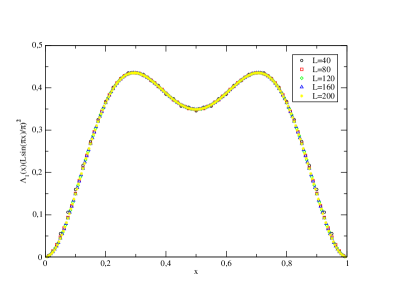
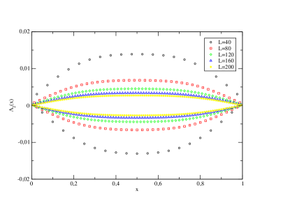
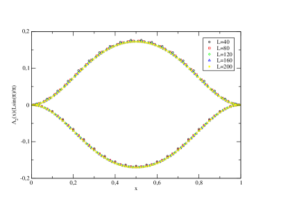
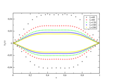
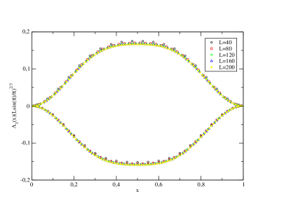
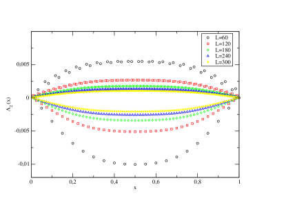
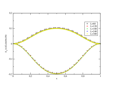
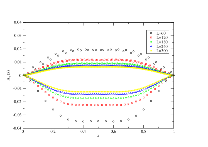
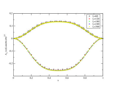
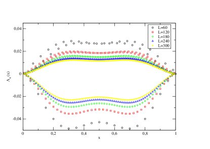
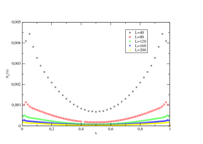
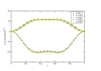
In Fig. III.1 we present the plots of Λn(x)subscriptΛ𝑛𝑥\Lambda_{n}(x) and the ones of (Lsin(πx)/π)2nΛn(x)superscript𝐿𝜋𝑥𝜋2𝑛subscriptΛ𝑛𝑥\left(L\sin(\pi x)/\pi\right)^{\frac{2}{n}}\Lambda_{n}(x) for different XX systems at half-filling. Data from systems with different values of L𝐿L are presented in the same plot for every value of n𝑛n to make an easier comparison between them. It is possible to see that the function Λn(x)subscriptΛ𝑛𝑥\Lambda_{n}(x) for fixed n𝑛n depends on the size of the system L𝐿L and it goes to zero with L𝐿L\rightarrow\infty. This represents the fact that in the thermodynamic limit the CFT result is exact and the corrections vanish. On the other side, (Lsin(πx)/π)2nΛn(x)superscript𝐿𝜋𝑥𝜋2𝑛subscriptΛ𝑛𝑥\left(L\sin(\pi x)/\pi\right)^{\frac{2}{n}}\Lambda_{n}(x) is no longer a function of L𝐿L and it depends just on the variable x=l/L𝑥𝑙𝐿x=l/L and on the filling, as we can see in the next figure.
Refer to caption
Refer to caption
(a)
Refer to caption
Refer to caption
(b)
Refer to caption
Refer to caption
(c)
Figure III.1: Plots of ΛnsubscriptΛ𝑛\Lambda_{n} (left) and (Lsin(πx)/π)2nΛnsuperscript𝐿𝜋𝑥𝜋2𝑛subscriptΛ𝑛\left(L\sin\left(\pi x\right)/\pi\right)^{\frac{2}{n}}\Lambda_{n} (right) computed for the particle-hole excited state in the half-filling XX models for different values of the system size L𝐿L. From the top to the bottom n=1𝑛1n=1, n=2𝑛2n=2 and n=3𝑛3n=3.

In Fig. III.2 the same quantities as before are plotted for ν=1/3𝜈13\nu=1/3 XX models for different values of the system size L𝐿L. The scaling of ΛnsubscriptΛ𝑛\Lambda_{n} is still the same as in the case ν=1/2𝜈12\nu=1/2, but a comparison between Λn(Lsin(πx)/π)2nsubscriptΛ𝑛superscript𝐿𝜋𝑥𝜋2𝑛\Lambda_{n}(L\sin\left(\pi x\right)/\pi)^{\frac{2}{n}} for ν=1/3𝜈13\nu=1/3 and ν=1/2𝜈12\nu=1/2 shows that they are not the same.
Refer to caption
Refer to caption
(a)
Refer to caption
Refer to caption
(b)
Refer to caption
Refer to caption
(c)
Figure III.2: Plots of ΛnsubscriptΛ𝑛\Lambda_{n} (left) and (Lsin(πx)/π)2nΛnsuperscript𝐿𝜋𝑥𝜋2𝑛subscriptΛ𝑛\left(L\sin\left(\pi x\right)/\pi\right)^{-\frac{2}{n}}\Lambda_{n} (right) computed for the particle-hole excited state in the ν=1/3𝜈13\nu=1/3 XX models for different system size L𝐿L. From the top to the bottom n=2𝑛2n=2, n=3𝑛3n=3 and n=4𝑛4n=4.

The previous analysis allows us to write the corrections in a more general way factorizing the scaling factor depending on L𝐿L from the function n(x;ν)subscript𝑛𝑥𝜈\mathcal{F}_{n}(x;\nu) which depends just on x=l/L𝑥𝑙𝐿x=l/L and on the filling factor.

Λn(x)=(Lsin(πx)π)2nn(x;ν)subscriptΛ𝑛𝑥superscript𝐿𝜋𝑥𝜋2𝑛subscript𝑛𝑥𝜈\Lambda_{n}(x)=\left(\frac{L\sin\left(\pi x\right)}{\pi}\right)^{-\frac{2}{n}}\mathcal{F}_{n}(x;\nu) (III.17)

We will study the function n(x;ν)subscript𝑛𝑥𝜈\mathcal{F}_{n}\left(x;\nu\right) in the next section, comparing the functions ΛnsubscriptΛ𝑛\Lambda_{n} found for the excited states with the ones computed exactly in the ground state case.

III.3 Comparison with non CFT results

The entanglement entropy of the XX model has been computed in several methods different from the replica trick one. In particular, in Ref.correzzioni ; correzzioni2 an analytic expression for the corrections to the continuum theory dn(N)Sn(N)Sna0subscript𝑑𝑛𝑁subscript𝑆𝑛𝑁superscriptsubscript𝑆𝑛𝑎0d_{n}(N)\equiv S_{n}(N)-S_{n}^{a\rightarrow 0} can be found. This result has been obtained with an explicit computation of the Rényi entropy which uses the properties of the Toeplitz determinants, see Ref. 351882944 .

dn(N)=2cos(2kFl)1n(2Nsin(πl/L))2/n[Γ(12+12n)Γ(1212n)]2.subscript𝑑𝑛𝑁22subscript𝑘𝐹𝑙1𝑛superscript2𝑁𝜋𝑙𝐿2𝑛superscriptdelimited-[]Γ1212𝑛Γ1212𝑛2d_{n}(N)=\dfrac{2\cos(2k_{F}l)}{1-n}\left(2N\sin(\pi l/L)\right)^{-2/n}\left[\dfrac{\Gamma\left(\frac{1}{2}+\frac{1}{2n}\right)}{\Gamma\left(\frac{1}{2}-\frac{1}{2n}\right)}\right]^{2}. (III.18)

Where it is easy to recognize the scaling factor of the unusual corrections to the scaling for the ground state with Δ=1Δ1\Delta=1. The method used in Ref. correzzioni ; correzzioni2 cannot be applied to the excited states, in this case our method is the only one that can predict the correct scaling of these corrections. We want now to study the dependence of these corrections on the filling factor ν𝜈\nu using the quantity

Rn(x)=(1n)(2π)2/n2cos(2kFl)[Γ(12+12n)Γ(1212n)]2n(x;ν).subscript𝑅𝑛𝑥1𝑛superscript2𝜋2𝑛22subscript𝑘𝐹𝑙superscriptdelimited-[]Γ1212𝑛Γ1212𝑛2subscript𝑛𝑥𝜈R_{n}(x)=\dfrac{(1-n)(2\pi)^{2/n}}{2\cos(2k_{F}l)\left[\dfrac{\Gamma\left(\frac{1}{2}+\frac{1}{2n}\right)}{\Gamma\left(\frac{1}{2}-\frac{1}{2n}\right)}\right]^{2}}\mathcal{F}_{n}(x;\nu). (III.19)

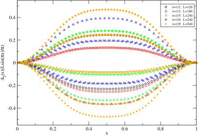
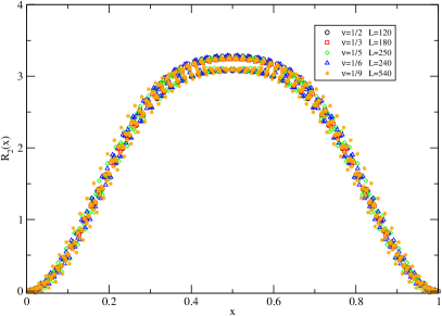
If the dependence on the filling ν𝜈\nu is the same in both dn(x)subscript𝑑𝑛𝑥d_{n}(x) and n(x;ν)subscript𝑛𝑥𝜈\mathcal{F}_{n}(x;\nu), their ratio will no longer depend on ν𝜈\nu and we the function Rn(x)subscript𝑅𝑛𝑥R_{n}(x) will be independent of ν𝜈\nu. In Fig. III.3 we plot the functions Λ2subscriptΛ2\Lambda_{2} and R2subscript𝑅2R_{2} obtained for different values of the ν𝜈\nu and L𝐿L parameters. It is possible to see that all the R2(x)subscript𝑅2𝑥R_{2}(x) functions collapse on the same curve.
Refer to caption
Refer to caption
Figure III.3: Left: Plots of the function Λ2(Lsin(πx)/π)1subscriptΛ2superscript𝐿𝜋𝑥𝜋1\Lambda_{2}\left(L\sin\left(\pi x\right)/\pi\right)^{-1} for different values of ν𝜈\nu and L𝐿L. Right: Plot of R2(x)subscript𝑅2𝑥R_{2}(x) for different values of ν𝜈\nu and L𝐿L. The excited state studied is the particle-hole

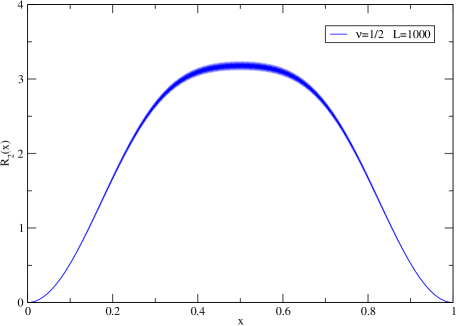
In Fig. III.4 we plot R2(x)subscript𝑅2𝑥R_{2}(x) for a much bigger system than the previous ones. This demonstrates that the residual oscillations in Fig. III.3 are due to finite size effects and they disappear in the thermodynamic limit. This confirms that Rn(x)subscript𝑅𝑛𝑥R_{n}(x) does not depend neither on L𝐿L neither on ν𝜈\nu.

Refer to caption
Figure III.4: Plot of the function R2(x)subscript𝑅2𝑥R_{2}(x) obtained using a half-filled chain of length L=1000𝐿1000L=1000. The excited state is the particle-hole state.

We demonstrated that the corrections to the entanglement entropy of the excited states are the same as the one of the ground state up to a function of l/L𝑙𝐿l/L, we demonstrated that it is possible to write these corrections in the general form

Λn=dn(N)Rn(x),subscriptΛ𝑛subscript𝑑𝑛𝑁subscript𝑅𝑛𝑥\Lambda_{n}=d_{n}\left(N\right)R_{n}(x), (III.20)

where dn(N)subscript𝑑𝑛𝑁d_{n}(N) are the corrections to the continuum theory in the ground state case and the function Rn(x)subscript𝑅𝑛𝑥R_{n}(x) is an unknown model dependent function which depends just on l/L𝑙𝐿l/L.

IV Conclusions & Outlooks

We demonstrated that the unusual corrections to the scaling of the entanglement entropy in the excited states of the conformal field theory are due to the local breaking of the conformal invariance around the conical singularities of the Riemann surface, as in the ground state case. Many terms contribute to these corrections but the dominant one scales as (Lsin(πx)/π)2Λnsuperscript𝐿𝜋𝑥𝜋2Λ𝑛\left(L\sin(\pi x)/\pi\right)^{-\frac{2\Lambda}{n}} where it is possible to admire the geometrical dependence of the scaling of these corrections. We checked our predictions using exact numerical computations of the entanglement entropy of the excited states of the XX model finding a perfect agreement. By comparing our numerical data with the exact analytical expression for these corrections in the ground-state found in Ref. correzzioni , we find that the dependence on the filling factor is the same both in the ground and the excited states.
In the future it would be interesting to compute the function Rn(x)subscript𝑅𝑛𝑥R_{n}(x) to see if it is model dependent or not. This can be done in the random XX model, where the entanglement entropy can be studied analytically for the ground and the excited states, see Ref. hopping1 ; hopping2 . Moreover, the study of the corrections to the CFT results can be done for Rieman surfaces different from the one considered in this work. The entanglement negativity between two disjoints subsystem A1subscript𝐴1A_{1} and A2subscript𝐴2A_{2} of a system S𝑆S has in fact proven to be described by a richer structure than the single interval case, Ref. neg1 ; neg2 ; neg3 , and the CFT result could be affected again by more complicated geometry dependent corrections.

Acknowledgments We thanks P. Calabrese, E. Ercolessi, L. Taddia, A. Fabbri, P. Mattioli for very helpful discussions. The author is supported by the ERC (FP7/2007-2013 Grant Agreement No. 256294).

References

  • (1) E. Schrödinger. Probability relations between separated systems. Mathematical Proceedings of the Cambridge Philosophical Society, 32, 1936.
  • (2) E. Schrödinger. Discussion of probability relations between separated systems. Mathematical Proceedings of the Cambridge Philosophical Society, 31, 1935.
  • (3) E. Schrödinger. Die gegenwartige situation in der quantenmechanik. Naturwissenschaften, 23(48), 1935.
  • (4) A. Einstein, B. Podolsky, and N. Rosen. Can quantum-mechanical description of physical reality be considered complete? Phys. Rev., 47, 1935.
  • (5) R. Horodecki, P. Horodecki, M. Horodecki, and K. Horodecki. Quantum entanglement. Rev. Mod. Phys., 81, 2009.
  • (6) M. Rinaldi. Entropy of an acoustic black hole in bose-einstein condensates. Phys. Rev. D, 84, 2011.
  • (7) I. Masafumi, L. Feng-Li, and N. Bo. Refined holographic entanglement entropy for the ads solitons and ads black holes. Nuclear Physics B, 872(3), 2013.
  • (8) T. Azeyanagi, T. Nishioka, and T. Takayanagi. Near extremal black hole entropy as entanglement entropy via ads2/cft1subscriptads2subscriptcft1{\mathrm{ads}}_{2}/{\mathrm{cft}}_{1}. Phys. Rev. D, 77, 2008.
  • (9) P. Shor. Polynomial-time algorithms for prime factorization and discrete logarithms on a quantum computer. SIAM Review, 41(2), 1999.
  • (10) L. Amico and R. Fazio. Entanglement and magnetic order. Journal of Physics A: Mathematical and Theoretical, 42(50), 2009.
  • (11) L. Amico, R. Fazio, A. Osterloh, and V. Vedral. Entanglement in many-body systems. Rev. Mod. Phys., 80, 2008.
  • (12) P. Di Francesco, P. Mathieu, and D. Sénéchal. Conformal Field Theory. Graduate Texts in Contemporary Physics. Springer New York, New York, NY, 1997.
  • (13) C. Holzhey, F. Larsen, and F. Wilczek. Geometric and renormalized entropy in conformal field theory. Nuclear Physics B, 424(3), 1994.
  • (14) G. Vidal, J. I. Latorre, E. Rico, and A. Kitaev. Entanglement in quantum critical phenomena. Phys. Rev. Lett., 90, 2003.
  • (15) P. Calabrese and J. Cardy. entanglement entropy and quantum field theory: a non-technical introduction. International Journal of Quantum Information, 04(03), 2006.
  • (16) P. Calabrese and J. Cardy. Entanglement entropy and conformal field theory. Journal of Physics A: Mathematical and Theoretical, 42(50), 2009.
  • (17) P. Calabrese and J. Cardy. Entanglement entropy and quantum field theory. Journal of Statistical Mechanics: Theory and Experiment, 2004(06), 2004.
  • (18) J. Cardy and I. Peschel. Finite-size dependence of the free energy in two-dimensional critical systems. Nuclear Physics B, 300, 1988.
  • (19) J. L. Cardy, O. A. Castro-Alvaredo, and B. Doyon. Form factors of branch-point twist fields in quantum integrable models and entanglement entropy. Journal of Statistical Physics, 130(1), 2008.
  • (20) M. I. Berganza, F. C. Alcaraz, and G. Sierra. Entanglement of excited states in critical spin chains. Journal of Statistical Mechanics: Theory and Experiment, 2012(01), 2012.
  • (21) F. C. Alcaraz, M. I. Berganza, and G. Sierra. Entanglement of low-energy excitations in conformal field theory. Phys. Rev. Lett., 106, 2011.
  • (22) J. I. Latorre and A. Riera. A short review on entanglement in quantum spin systems. Journal of Physics A: Mathematical and Theoretical, 42(50), 2009.
  • (23) B-Q. Jin and V. E. Korepin. Quantum spin chain, toeplitz determinants and the fisher?hartwig conjecture. Journal of Statistical Physics, 116, 2004.
  • (24) A. R. Its, B-Q. Jin, and V. E. Korepin. Entanglement in the xy spin chain. Journal of Physics A: Mathematical and General, 38(13), 2005.
  • (25) V. E. Korepin. Universality of entropy scaling in one dimensional gapless models. Phys. Rev. Lett., 92, 2004.
  • (26) J. P. Keating and F. Mezzadri. Random matrix theory and entanglement in quantum spin chains. Communications in Mathematical Physics, 252(1-3), 2004.
  • (27) T. Barthel, M-C. Chung, and U. Schollwöck. Entanglement scaling in critical two-dimensional fermionic and bosonic systems. Phys. Rev. A, 74, 2006.
  • (28) G. De Chiara, S. Montangero, P. Calabrese, and R. Fazio. Entanglement entropy dynamics of heisenberg chains. Journal of Statistical Mechanics: Theory and Experiment, 2006(03), 2006.
  • (29) F. Iglói and R. Juhász. Exact relationship between the entanglement entropies of xy and quantum ising chains. EPL (Europhysics Letters), 81(5), 2008.
  • (30) B. Nienhuis, M. Campostrini, and P. Calabrese. Entanglement, combinatorics and finite-size effects in spin chains. Journal of Statistical Mechanics: Theory and Experiment, 2009(02), 2009.
  • (31) V. Alba, M. Fagotti, and P. Calabrese. Entanglement entropy of excited states. Journal of Statistical Mechanics: Theory and Experiment, 2009(10), 2009.
  • (32) I. Peschel and V. Eisler. Reduced density matrices and entanglement entropy in free lattice models. Journal of Physics A: Mathematical and Theoretical, 42(50), 2009.
  • (33) E. Ercolessi, S. Evangelisti, F. Franchini, and F. Ravanini. Correlation length and unusual corrections to entanglement entropy. Phys. Rev. B, 85, 2012.
  • (34) P. Calabrese, J. Cardy, and I. Peschel. Corrections to scaling for block entanglement in massive spin chains. Journal of Statistical Mechanics: Theory and Experiment, 2010(09), 2010.
  • (35) P. Calabrese, M. Campostrini, F. Essler, and B. Nienhuis. Parity effects in the scaling of block entanglement in gapless spin chains. Phys. Rev. Lett., 104, 2010.
  • (36) P. Calabrese and F. H. L. Essler. Universal corrections to scaling for block entanglement in spin-1/2 xx chains. Journal of Statistical Mechanics: Theory and Experiment, 2010(08), 2010.
  • (37) N. Laflorencie, E. S. Sørensen, M-S. Chang, and I. Affleck. Boundary effects in the critical scaling of entanglement entropy in 1d systems. Phys. Rev. Lett., 96, 2006.
  • (38) H. F. Song, S. Rachel, and K. Le Hur. General relation between entanglement and fluctuations in one dimension. Phys. Rev. B, 82, 2010.
  • (39) L. Taddia, J. C. Xavier, F. C. Alcaraz, and G. Sierra. Entanglement entropies in conformal systems with boundaries. Phys. Rev. B, 88, 2013.
  • (40) M. Dalmonte, E. Ercolessi, and L. Taddia. Critical properties and rényi entropies of the spin-3232\frac{3}{2} xxz𝑥𝑥𝑧xxz chain. Phys. Rev. B, 85, 2012.
  • (41) M. Dalmonte, E. Ercolessi, and L. Taddia. Estimating quasi-long-range order via rényi entropies. Phys. Rev. B, 84, 2011.
  • (42) M. Fagotti and P. Calabrese. Universal parity effects in the entanglement entropy of xx chains with open boundary conditions. Journal of Statistical Mechanics: Theory and Experiment, 2011(01), 2011.
  • (43) J. C. Xavier and F. C. Alcaraz. Rényi entropy and parity oscillations of anisotropic spin-s𝑠s heisenberg chains in a magnetic field. Phys. Rev. B, 83, 2011.
  • (44) E. Eriksson and H. Johannesson. Corrections to scaling in entanglement entropy from boundary perturbations. Journal of Statistical Mechanics: Theory and Experiment, 2011(02), 2011.
  • (45) J. Cardy and P. Calabrese. Unusual corrections to scaling in entanglement entropy. Journal of Statistical Mechanics: Theory and Experiment, 2010(04), 2010.
  • (46) P. Calabrese, M. Mintchev, and E. Vicari. The entanglement entropy of one-dimensional systems in continuous and homogeneous space. Journal of Statistical Mechanics: Theory and Experiment, 2011(09), 2011.
  • (47) P. Calabrese, M. Mintchev, and E. Vicari. Entanglement entropy of one-dimensional gases. Phys. Rev. Lett., 107, 2011.
  • (48) E. Ardonne and G. Sierra. Chiral correlators of the ising conformal field theory. Journal of Physics A: Mathematical and Theoretical, 43(50), 2010.
  • (49) F. H. L. Essler, A. M. Läuchli, and P. Calabrese. Shell-filling effect in the entanglement entropies of spinful fermions. Phys. Rev. Lett., 110, 2013.
  • (50) P. Calabrese, F. H. L. Essler, and A. M. Läuchli. Entanglement entropies of the quarter filled hubbard model. Journal of Statistical Mechanics: Theory and Experiment, 2014(9), 2014.
  • (51) G. Ramírez, J. Rodríguez-Laguna, and G. Sierra. Entanglement in low-energy states of the random-hopping model. Journal of Statistical Mechanics: Theory and Experiment, 2014(7):P07003, 2014.
  • (52) M. Fagotti, P. Calabrese, and J. E. Moore. Entanglement spectrum of random-singlet quantum critical points. Phys. Rev. B, 83, 2011.
  • (53) P. Calabrese, J. Cardy, and E. Tonni. Entanglement negativity in quantum field theory. Phys. Rev. Lett., 109, 2012.
  • (54) P. Calabrese, J. Cardy, and E. Tonni. Entanglement negativity in extended systems: a field theoretical approach. Journal of Statistical Mechanics: Theory and Experiment, 2013(02):P02008, 2013.
  • (55) P. Calabrese, J. Cardy, and E. Tonni. Finite temperature entanglement negativity in conformal field theory. Journal of Physics A: Mathematical and Theoretical, 48(1), 2015.