Fixed-point algorithms for frequency estimation and structured low rank approximation
Abstract
We develop fixed-point algorithms for the approximation of structured matrices with rank penalties. In particular we use these fixed-point algorithms for making approximations by sums of exponentials, or frequency estimation. For the basic formulation of the fixed-point algorithm we show that it converges to the minimum of the convex envelope of the original objective function along with its structured matrix constraint. It often happens that this solution agrees with the solution to the original minimization problem, and we provide a simple criterium for when this is true. We also provide more general fixed-point algorithms that can be used to treat the problems of making weighted approximations by sums of exponentials given equally or unequally spaced sampling. We apply the method to the case of missing data, although optimal convergence of the fixed-point algorithm is not guaranteed in this case. However, it turns out that the method often gives perfect reconstruction (up to machine precision) in such cases. We also discuss multidimensional extensions, and illustrate how the proposed algorithms can be used to recover sums of exponentials in several variables, but when samples are available only along a curve.
Keywords: Fixed-point algorithms, Frequency estimation. General domain Hankel matrices, Fenchel conjugate, Convex envelope.
Mathematics Subject Classification: 15B05, 65K10, 41A29, 41A63.
1 Introduction
We consider the non-convex problem
| (1) |
where is an -matrix, any linear subspace, is a parameter and the norm refers to the Frobenius norm. The convex envelope of is then given by
| (2) |
where
see [19, 20] for details. We provide a fixed point algorithm which is guaranteed to solve the problem
| (3) |
for any and . It turns out that the solution to (3) often coincides with the solution to the non-convex problem (1) for , and we provide a simple condition to verify if this has happened. To be more precise, below is a compilation of Theorem 5.1 and Theorem 5.2 in the particular case for the non-linear map defined by (23).
Theorem 1.1.
To provide more flexibility in choosing the objective functional, we also consider the problem of minimizing
| (4) |
where is a linear operator into any given linear space. We give conditions under which the fixed points of a certain non-linear operator coincide with the global minimum of this problem.
We apply these algorithms to the problem of approximation by sparse sums of exponentials. Let be the function that we wish to approximate, and assume that it is sampled at points . The problem can then be phrased as
| (5) |
Here, the parameter is a parameter that penalizes the number of exponential functions. The weights can be used to control the confidence levels in the samples .
This approximation problem is closely related to the problem of frequency estimation, i.e., the detection of the (complex) frequencies above. Once the frequencies are known, the remaining approximation problem becomes linear and easy to solve by means of least squares. The literature on frequency estimation is vast. The first approach was made already in 1795 [16]. Notable methods that are commonly used are ESPRIT [25], MUSIC [27] and matrix pencil methods [17]. We refer to [28] for an overview from a signal processing perspective. From an analysis point of view, the AAK-theory developed in [1, 2, 3] deals with closely related problems, and approximation algorithms based on these results were developed in [9, 14]. A competitive algorithm in the case of fixed was recently developed in [11].
To approach this problem, we let denote the set of Hankel matrices, i.e., if , then there is a generating function such that . Hankel matrices are thus constant along the anti-diagonals. By the Kronecker theorem there is a connection between a sums of exponential functions and Hankel matrices with rank , namely that if is a linear combination of exponential functions sampled at equally spaced points, then the Hankel matrix generated by these samples will generically have rank . For more details, see e.g. [4, 5, 18, 23].
In the special case with equally spaced sampling, i.e. , and
| (6) |
the problem (5) (with being the Hankel matrix generated from ) is equivalent with (2). The triangular weight above comes from counting the number of elements in the Hankel matrix along the anti-diagonals. Theorem 1.1 thus provide approximate solutions to this problem, which often turn out to solve the original problem (5) as well, which in this setting is the equivalent of (1).
Clearly, for many purposes it would be more natural to use the regular norm in the approximation, i.e., to use constant values of . Also more general setups of weights can be of interest (for instance in the case of missing data). We show how the fixed-point algorithm designed for (4) can be used in this case.
The basic algorithms for frequency estimation (or approximations by sums of exponentials) require that the data is provided (completely) at equally spaced samples. In many situations, this assumption does not hold (in particular concerning sampling in two or more variables). A traditional method designed for computing periodograms for unequally spaced sampling is the Lomb-Scargle method [21, 26]. The results are typically far from satisfactory, cf. [11]. For a review of frequency estimation methods for unequally spaced sampling, see [12]. In this work, we will use similar ideas as in [11] for treating the unequally spaced sampling. Given a set of sample points , let be a matrix that interpolates between equally spaced points and the points . This means for instance that the rows of have sum one. The action of its adjoint is sometimes referred to as anterpolation. We study the problem
| (7) |
using the algorithm for (4), and we also modify (7) to deal with the corresponding weighted case.
Finally, we discuss how the methods can be used in the multidimensional case. Let be an open bounded connected set and a function on which is assumed to be of the form
| (8) |
where , and is a low number. In [4] we introduce a new class of operators called general domain truncated correlation operators, whose “symbols” are functions on , and prove a Kroncker-type theorem for these operators. In particular it follows that their rank is if the symbol is of the form (8), and the converse situation is also completely clarified. In [5] it is explained how these operators can be discretized giving rise to a class of structured matrices called “general domain Hankel matrices”, (see Section 7 for more details). Letting be such a class of structured matrices, it turns out that (3) is a natural setting for solving the problem: Given noisy measurements of at (possibly unequally spaced) points in , find the function . The connected problem of finding the values and is addressed e.g. in [6].
The paper is organized as follows: In Section 2 we provide some basic ingredients for the coming sections, in particular we introduce the singular value functional calculus and connected Lipschitz estimates. Our solution of (3) involves an intermediate more intricate objective functional, which is introduced in Section 3, where we also investigate the structure of its Fenchel conjugates. Moreover our solution to (3) first solves a dual problem, which is introduced and studied in Section 4. Consequently the key operator is introduced in Section 4. At this point, we have the ingredients necessary for addressing the main problem (3). In Section 5.1 we recapitulate our main objective and discuss how various choices of and affect the objective functional and also its relation to the original problem (1). An extended version of Theorem 1.1 is finally given in Section 5.2, where we also present our algorithm for solving (3). The more general version of the algorithm and corresponding theory is given in Section 5.3. The remainder of the paper is devoted to frequency estimation and numerical examples. Section 6 considers the one-dimensional problem (7), whereas the problem of retrieving functions of the form (8) is considered in Section 7. This section also contains a more detailed description of the general domain Hankel matrices which underlies the method. Numerical examples are finally given in Section 8 and we end with a summary of our conclusions in Section 9.
2 Preliminaries
2.1 Fenchel conjugates and convex optimization
We recall that the Fenchel conjugate of a function is given by
For positive functions , is always convex, and if is also convex, then , see Theorem 11.1 in [24]. If is not convex, then equals the convex envelope of . In particular, note that we always have .
Suppose now that is a convex function on some finite dimensional linear space , and let be a linear subspace. Consider the problem of finding
| (9) | ||||
If then the value in (9) is clearly larger than or equal to the value
| (10) |
Suppose now that we can find a value (not necessarily unique) which minimizes
| (11) | ||||
Since is convex, it is easy to see that the corresponding value in (10) equals that of (9).
2.2 The singular value functional calculus
Let be given and let denote the Euclidean space of -matrices, equipped with the Frobenius norm. We will need the singular value functional calculus [10], defined as follows. Let be a real valued function on such that and let be a matrix with singular value decomposition . We then define
The key property we will use is that
| (12) |
where refers to the Lipschitz constant for . In other words, Lipschitz functions give rise to Lipschitz functional calculus, with the same bound.
3 Convex envelopes
Theorem 3.1.
Let be a fixed matrix, and let
| (13) |
The Fenchel conjugates of are then
| (14) | ||||
| (15) |
Let and let be conjugate exponents, i.e. such that .
Theorem 3.2.
Let
It’s Fenchel conjugate is then given by
| (16) |
and its convex envelope (Fenchel bi-conjugate) is given by
| (17) |
Proof.
We write simply when are clear from the context. Consider the Fenchel conjugate of
The right maximum is attained for
After substituting in the Fenchel conjugate and some algebraic simplifications, we obtain
From (14) we see that the expression inside the first parenthesis can be written as
from which (16) follows.
Next we study the bi-conjugate
To simplify the computations we change coordinates
| (18) |
for which
The bi-conjugate can then be written as
The maximization over is straightforward and it will give a contribution for . Hence by (18), and
We recognize the maximization part as a Fencel conjugate, and hence
4 The dual optimization problem
Let be any fixed linear subspace. We consider the problem
| (19) | ||||
where . Let be the linear subspace of defined by the equations and . It is easy to see that is defined by
Indeed, is obvious and the other part can be established by noting that whereas the subspace defined by has dimension , (which thus equals ). Motivated by the results in Section 2.1, we now focus on the “dual problem” to (19), i.e.
| (20) | ||||
Set
| (21) |
When there is no risk for confusion we will omit the subindices. Recall the singular value functional calculus introduced in Section 2.2.
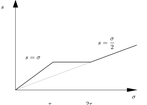
Lemma 4.1.
Proof.
Since depends only on the singular values of , von-Neumann’s inequality [29] shows that the solution to the above problem will have the same singular vectors as , (see the proof of Theorem 3.1 in [10] for more details). Henceforth it will be of the form where is defined by
| (22) |
and by equating the subgradient of the above expression with respect to with zero, it is easily verified that this is solved by the function (21). ∎
Let denote the operator of orthogonal projection onto . We now introduce the (non-linear) operator which will play a key role in our solution of the original problem (3).
Definition 4.2.
Set
| (23) |
which we abbreviate when are clear from the context.
Theorem 4.3.
There exists a fixed point of such that the problem
| (24) | ||||||
| subject to |
is solved by
| (25) | ||||
Proof.
Since we can write
with and . By (16) the problem (24) becomes
Note that
where . The problem can thus be rewritten
Since and , it follows that
and hence we conclude that the optimal is the zero matrix. Thus
and the objective functional can be replaced by
Using the substitution it then becomes
The minimization problem will thus be solved by
| (26) |
where is the functional defined by
Note that is convex since it is obtained from the convex function by affine changes of coordinates. It is also easy to see that
so it has at least one global minimum. Let be one such. Since , it is easy to see that . But then
which by Lemma 4.1 read
It is also evident that is a solution to (26). The formulas in (25) now follows by tracing the changes of variables backwards. ∎
5 A fixed point algorithm
5.1 Discussion of the objective functional
To recapitulate our main objective, we wish to minimize
| (27) |
which we replace by its convex envelope
| (28) |
to achieve convexity. We will in this section show how to minimize
| (29) |
for any and . Note that the corresponding modification to the original objective functional (27), i.e.
| (30) |
does not change the problem, since we may equivalently solve (27) with (to see this, multiply (30) with ). However, this is not the case with (29), for it is easy to show that
Thus (29) is equivalent with
| (31) |
where , compare with (27) and (28). Note as well that
by which we conclude that the objective functional in (29) is strictly convex with a unique minimizer . Moreover, the above expression is clearly less than or equal to
so if it happens that
| (32) |
then is a solution to the original problem (30). However, by the definition of it follows that (32) is satisfied if and only if has no singular values in the interval .
5.2 The basic fixed-point algorithm
We now solve (29), using fixed points of the operator from the previous section. It is easy to see that these may not be unique. Despite that, we have the following.
Theorem 5.1.
The Picard iteration converges to a fixed point . Moreover, is unique and
is the unique solution to (29).
Before the presenting the proof, let us give a few more comments on the equivalent problem formulation (31). Note that
but that our method requires (in fact, the objective functional is no longer convex beyond ). However, choosing will yield slow convergence of the Picard iteration since then . On the other hand, the effect of choosing a large (for a fixed ) is that the term deviates further from . We have found that works well in practice.
Proof.
We first prove that the Picard iteration converges. Note that the sequence , is generated by the Picard iteration of the operator and the starting-point . Moreover . Since is continuous (in fact, it is non-expansive by (12)) it suffices to show that is convergent.
It is well known [15, 22] that for firmly non-expansive operators (in finite dimensional space) the Picard iteration converges to a fixed point as long as the set of fixed points of the operator is non-empty. By Theorem 4.3 there exists a fixed point of , and it clearly follows that is a fixed point of . It remains to show that is firmly non-expansive, as an operator on . An equivalent to firmly non-expansive is that is non-expansive [13], i.e.,
| (33) |
which we will verify shortly. To this end, note that on we have
| (34) |
and set
This function is clearly Lipschitz continuous with Lipschitz constant equal to one. Setting and , (12) and (34) implies that
which establishes (33), and hence the original Picard iteration converges to a fixed point of . For the uniqueness of , suppose that is another fixed point of and write , where and . Then
where the last inequality is due to (12) and the fact that has Lipschitz constant equal to one. But then
implying that Finally, if denotes the solution to (19), then it is clear that solves (29). By the theory in Section 2.1 and Theorem 4.3, it follows that also is a solution to
| (35) | ||||
where is as above. By fixing we find that
| (36) | ||||
But inserting the constraint (from (19)) in the above equation yields
| (37) |
as desired. The uniqueness of was argued before the proof, so it is complete. ∎
The matrix has several peculiar properties, as shown by the next theorem, (compare with (29) and note the absence of the condition below).
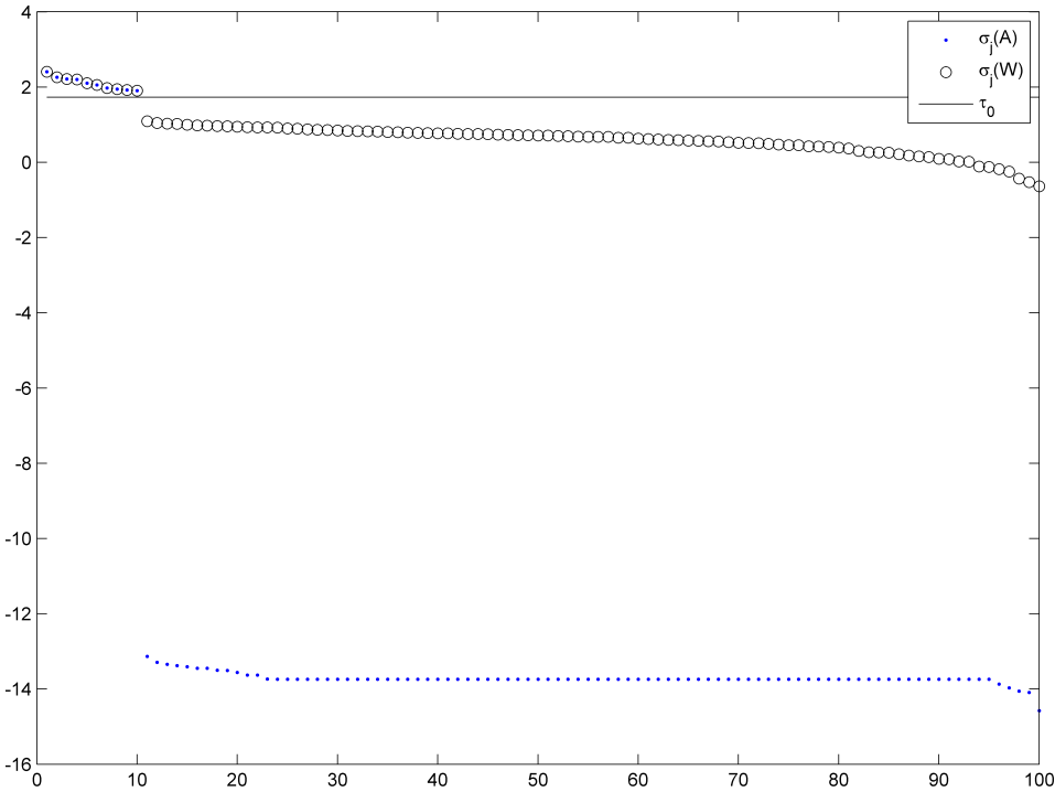
Theorem 5.2.
Proof.
By (36), minimizes (35) restricted to the subspace . By inserting this expression for in (36) and by a completion of squares, we get
Since only depend on the singular values of , it follows by von-Neumann’s inequality [29] that it is sufficient to consider the minimization of
| (39) |
The derivative of the function to be minimized is for and for , by which (38) easily follows. The final statement is immediate by the discussion in Section 5.1. ∎
5.3 The general fixed-point algorithm
In this Section we introduce a more general algorithm which allows increased flexibility. Examples of applications will be given in the coming sections. Let be an Euclidean space and let be a linear operator. Given define
by
When there is no risk of confusion we will omit the subindices from the notation, and we will let denote the identity operator on .
Theorem 5.3.
Let be such that . Then there exists such that is a fixed point of if and only if is a stationary point of the objective functional
| (40) |
(as a functional on ). The objective functional is convex if , and strictly convex if .
Proof.
The statements about convexity follows from the identity
and the fact that is defined so that becomes convex (but not strictly convex). A stationary point of (40) is clearly stationary also for
| (41) |
The objective function can be rewritten
| (42) |
where is a remainder. Note that this is convex in . Theorem 5.1 implies that there exists a fixed point to such that
is a minimizer of (42). Moreover the theorem says that this minimizer is unique, so there can be no other stationary points to the functional. Hence
and thus is a fixed point of . Conversely, let be a fixed point of . Then, by following the earlier argument backwards, we see that solves (41). Since the differential of the last term is zero at , the subdifferential of the former two is zero as well, so is a stationary point of (40).
∎
6 Complex frequency estimation
If we let be the subspace of Hankel matrices, then the algorithm in Section 5.2 immediately yields a method for frequency estimation, (see e.g. [23], [11] or [5] for the connection between this problem and frequency estimation). We now show how the more general version in Section 5.3 can be used to deal with weights or unequally spaced points. The former case is simpler so we present that separately. We also only consider the case of square matrices, although it is perfectly possible to have them non-square. In our experience, the square case works better though.
Let be defined by
| (43) |
i.e. the operator that takes a sequence and forms the corresponding Hankel matrix. The adjoint is then given by
Set
| (44) |
and note that . Let be the sequence whose th element is , and note that is the operator that projects on and then forms the corresponding sequence , i.e. it acts as a (left)-inverse of the operation (43). In the remainder, we will usually write simply in place of , when there is no risk of confusion.
Corollary 6.1.
Let be positive weights and assume that (interpreted pointwise). Set
and set
Let be defined by
Then, there exists such that is a fixed point of if and only if is a stationary point of the objective functional
| (45) |
The objective functional is convex if , and strictly convex if .
Proof.
We apply Theorem 5.3 with and . Since , it is easy to see that the objective functional (40) transforms into (45) when applied to the variable . Let be the vector with value on the :th position and zeroes elsewhere, and define . Note that is a orthonormal basis in , and that with respect to this basis turns into a diagonal matrix whose diagonal elements are . By this it easily follows that the conditions on in Theorem 5.3 transforms into those stated above. It also follows that
| (46) |
and that
Consequently, it holds that
and therefore . ∎
Given a set of sample points , let be the space of functions on the set . We think of these as sequences on , and make identification with . Similarly, let be an equally spaced grid near , and let functions on be identified with . Let be an operator that interpolates between functions on and functions on . The action of its adjoint is sometimes referred to as anterpolation.
Corollary 6.2.
Let be positive weights and choose such that
Let
and let
Let be defined by
Then, there exists such that is a fixed point of if and only if is a stationary point of the objective functional
| (47) |
The objective functional is convex if , and strictly convex if the inequality is strict.
Proof.
The proof is made analogously to the proof of Corollary 6.1 by choosing and . ∎
7 Multidimensional frequency estimation on general domains
We now generalize the above framework to several variables. The most straightforward way to do this would be to introduce block-Hankel matrices. However, we aim at having a framework that is more flexible, and for that reason we will work with general domain Hankel matrices. To explain the main idea, note that a Hankel matrix can be realized as the operator given by
| (48) |
The bold notation is chosen for consistency with the notation used in [5]. This formulation is suitable to generalize to the several variable setting. Let and be open bounded and connected domains in . Given sampling lengths , consider the following (non-rectangular) grids
and analogously
i.e., and are grids covering the respective domains, and the grid lengths are implicit in the notation.
We define to be the Hilbert space of all functions with the norm
Moreover set
Given , we define, in analogy with (48), the general domain Hankel operator as the summing operator given by
| (49) |
We may of course represent as a vector, by ordering the entries in some (non-unique) way. More precisely, let denote the amount of elements in , and pick any bijection
| (50) |
The bijection could for example be the lexicographical ordering of the elements in . We can then identify with the vector given by
Letting be an analogous bijection for , it is clear that can be represented as a matrix, where the ’th element is . If both and are squares in , these matrices are just standard block-Hankel matrices. A larger discussion of their structure is found in [5], see in particular Section 4.
Let be the map that sends a function to its corresponding generalized domain Hankel matrix;
and let be the range of this operator. Theorem 5.1 then applies and provides a minimizer to (29). Note that
| (51) | ||||
where the weight-function evaluated at a point simply is the amount of times that the value appears in the matrix , in analogy with (44).
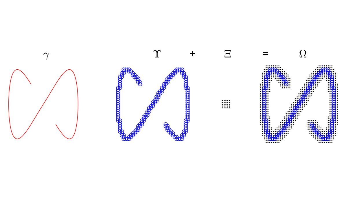
In Figure 3 we illustrate how a general domain Hankel matrix could be constructed. Suppose that we have data available along some subset of , in this case along a line . We want to inscribe the curve in a subset of an equally spaced grid . We would like to factorize the set as above. The generating values for the general domain Hankel matrix will in this case “live close” to where we have data. This is of particular importance if the exponential functions that we want to recover have frequencies with non-zero real part, as they easily can become huge far away from where the samples are available. The shape of the domain will control how many exponential functions that can be recovered. We refer to [7, 8] for details about how to recover the exponentials and the relationship between the size of and the number of exponential functions that can be recovered.
8 Numerical simulations
8.1 Equally spaced data
We begin with studying the case of equally spaced samples without weights. For this case the standard methods for frequency estimation are applicable. We will conduct some comparison of the results obtained by the proposed method against the results obtained by the ESPRIT method [25]. One difference between the proposed method and the ESPRIT method is that the number of exponentials sought for is predetermined in ESPRIT, while in the proposed method a penalty level is used instead of prescribing the number of exponentials. By modifying the penalty level , i.e., by modifying in (21), we can adapt the fixed point algorithms for making approximations using a fixed number of exponential functions. The simplest way to do this is to choose such that , if is the number of exponentials sought for. Note that the fixed point operator is then modified in between iterations, and that the convergence results are not directly applicable.
To avoid this difficulty, we will conduct experiments on sums of exponentials of the form (5) with . If the data is contaminated by noise, then the number of exponentials found can easily vary form small signal to noise ratios, if the strength (i.e. ) of the different exponentials have large variations.
We conduct experiments on a function of the form (5) with frequencies and coefficients given in Table 2 for .
| -23.141i | -3.1416i | 2.7183i | 31.006i | |
| 1.00000 | 0.62348+0.78183i | -0.22252+0.97493i | -0.90097+0.43388i |
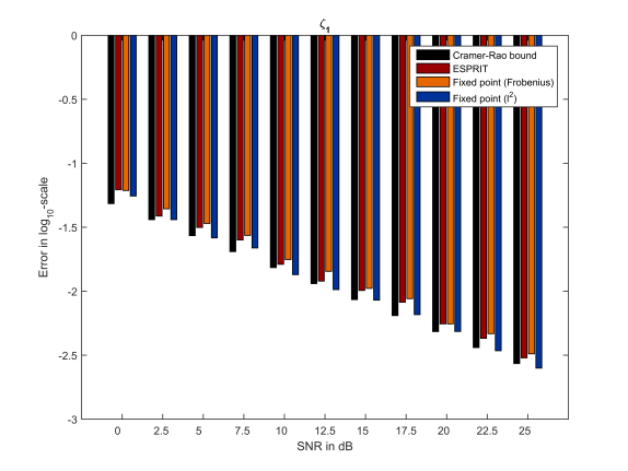

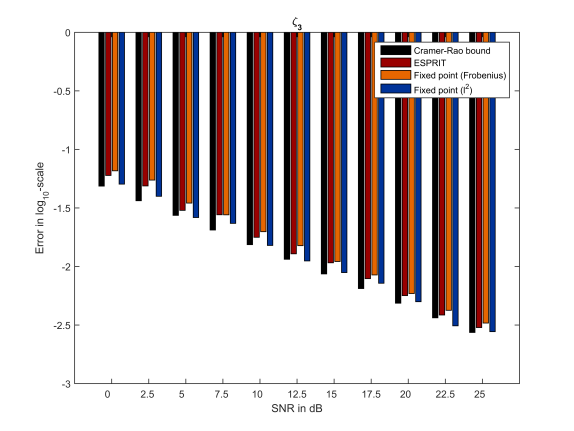
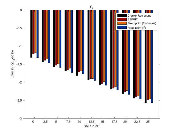
The function is sampled at 257 points, and white noise is added with different signal-to-noise rations (SNR). We test the fixed point algorithm given in Theorem 5.1 for a Frobenius norm error, and using the fixed point algorithm given in Corollary 6.1, for the standard norm. In Figure 4 we show the errors in recovering the frequencies from Table 2 for the two fixed point algorithms, along with the errors obtained from ESPRIT and the Cramér-Rao bound for the estimates. We can see that in comparison to the Frobenius based fixed point algorithm, the ESPRIT method works better in estimating the frequencies, but also that the version works better than ESPRIT. For this function, all three methods work well, and the obtained errors are close to the Cramér-Rao bound. Note that the methods are trying to optimize the approximation error of the function using few exponentials rather than estimating the frequencies present in the signal.
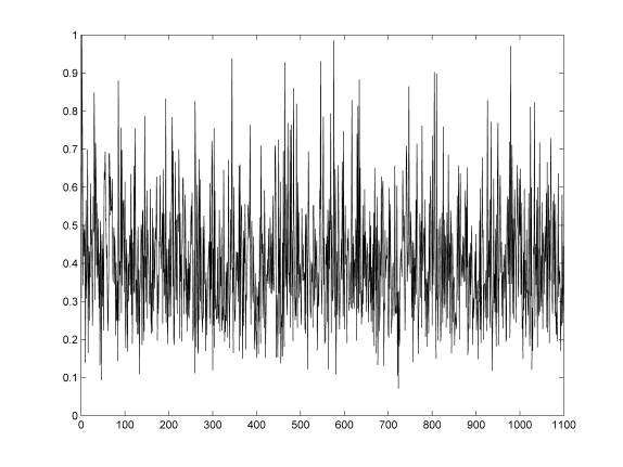
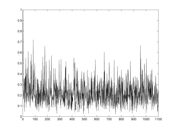
In Figure 5 we compare the approximation errors for the two methods against that or ESPRIT. The errors depicted are
and
respectively, where denotes the outcome from the fixed-point algorithm in Theorem 5.1, and the output of the fixed-point algorithm in Corollary 6.1. The errors are computed for the 11 different SNR values of Figure 4 using 100 simulation for each value. The errors are then normalized in relation to the SNR for the sake of visualizing them simultaneously. The scale on the -axis is thus a relative scale, and we have rescaled it so that the largest difference between the errors produced by the different methods is one. We can see that for both cases the errors are positive, meaning that the approximations obtained by the two fixed point methods consequently produce approximations with smaller error in the respective norm.
.
8.2 Missing data
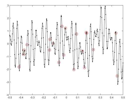
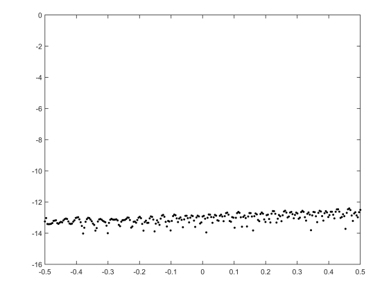
In this subsection we study the performance of the proposed method in the case of missing data. We assume that the samples are known only at a subset of an equally spaced sampling in one dimension. The function we study is the same as before, i.e. composed from the coefficients and frequencies given in Table 2. In the first test, we try to recover the function in the absence of noise, but with only few measurements available. The function is originally sampled at 257 points at one the interval , and we assume that only the 20 samples with indices
are known (these are randomly chosen). The real part of the original function is shown in black in the left panel of Figure 6, and the available data is illustrate by red circles. In the left panel the point-wise error between the reconstruction and the original function is shown in logarithmic scale. We can see that the reconstruction is accurate up to machine precision. Note that since , this is not guaranteed from Corollary 6.1. However, comparatively few samples are typically needed for the method to achieve perfect recovery in the absence of noise.
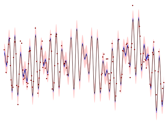
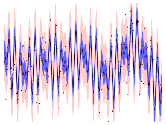
Next, we consider the same function but now noise is added. Half of the samples are kept (129 points). Moreover, the sampling points are chosen so that there is a gap on the interval . We conducted two sets of simulations, one for SNR=10 and one for SNR=0, and for both noise levels we ran the simulations 100 times. In Figure 7 we illustrate the results. The original function is displayed by the black curve, and for each of the figures, the red dots indicate the noise realization for one simulation. Note that the samples (red dots) deviate quite a lot from the true data. The pink shaded area illustrate the standard deviations for the the noise, and the blue shaded area illustrate the standard deviation of the errors from the obtained approximations. We can see that the errors in the reconstructions are substantially smaller than the original noise level. A similar experiment can also be done using the unequally spaced sampling formulation dealt with in Corollary 6.2.
8.3 Two-dimensional recovery along a curve
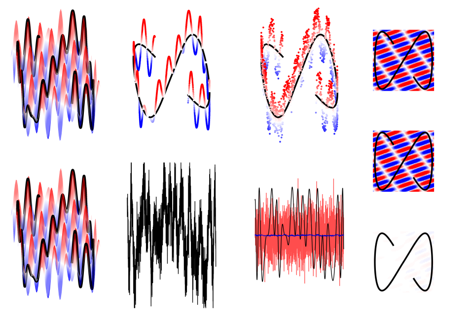
Next, we consider the case of unequally spaced sampling in two dimensions. In particular, we will choose points densely sampled along a curve. There are no particular constraints of the method that limits it to such sampling, it is simply an interesting and comparatively difficult problem. We will use the same curve as the one () shown in Figure 3. Due to the problems of satisfying the convexity constraints in Corollary 6.2, the algorithm can converge to for instance a zero solution. To avoid problems of this type, we assume that the number of exponential functions is known in advance and choose at each iteration.
In a first example we try out the proposed method in the case with exponential functions in two variables. The underlying function is shown at the top left panel of Figure 8. The black curve indicates the curve along which sampling is conducted. The sampling setup is also illustrated in the second (top) panel. Here the sampling curve () is indicated in black, and the sampled data values along the curve are illustrated by red, white and blue (densely sampled) dots. We perturb data by noise. For this case we apply a rather high level of noise, in particular Gaussian white noise with SNR=1 dB. The noisy measurements are illustrated in the third (top) panel from the left. We now apply the fixed-point algorithm. Upon convergence, we use the singular vectors on the (square) -domain to obtain frequency estimates following the strategy described in [7]. The corresponding coefficients can then be found by the least squares method. Once the frequencies and coefficients have been retrieved, we can reconstruct the underlying two-dimensional function. The result is shown in the bottom left panel. The second bottom panel show the measured (noisy) signal (along ); The third (bottom) panel show the noise-free signal in black; the noise itself in red; and the residual between the noise-free and the reconstructed signals in blue. The right column of panels of Figure 8 show in top views from top to bottom: the noise-free data; the reconstruction; and the corresponding residual. We can see that a rather good reconstruction was obtained, despite the high noise-level. This is partially because the original data set consisted of only two exponential functions.
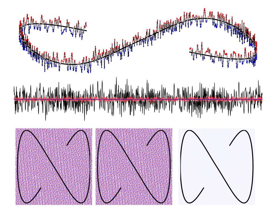
We now try the same problem but instead with exponential functions and an SNR of 5 dB. The top panel show the data sampled along the curve as before. We can see that the data looks substantially more complicated in this case. The same procedure as for the previous example is now applied. The middle panel show the noise-free data along in black and the corresponding residual with regards to the reconstruction in blue. The noise is shown in red. The three bottom panels show top views of the noise-free data; the reconstruction; and the corresponding residual for the underlying two-dimensional function. Finally, we provide the original and estimated frequencies for this two-dimensional case in Table 3.
| -50.0000 + 0.i | -50.0000 + 0.i | -50.0031 + 0.00265i | -49.9989 + 0.00255i |
| -42.5903 + 0.i | +12.8766 + 0.i | -42.5882 + 0.00118i | +12.8765 - 0.00100i |
| -35.1806 + 0.i | +40.7788 + 0.i | -35.1817 + 0.00142i | +40.7763 - 0.00027i |
| -20.3613 + 0.i | -2.72062 + 0.i | -20.3618 + 0.00278i | -2.72020 - 0.00275i |
| -6.67724 + 0.i | -34.2402 + 0.i | -6.67772 - 0.00267i | -34.2389 + 0.00089i |
| +4.98657 + 0.i | -42.4351 + 0.i | +4.98607 - 0.00091i | -42.4358 + 0.00056i |
| +9.27734 + 0.i | +18.0841 + 0.i | +9.27612 - 0.00129i | +18.0857 - 0.00397i |
| +19.4458 + 0.i | -9.77757 + 0.i | +19.4469 + 0.00072i | -9.77517 - 0.00032i |
| +36.6455 + 0.i | -27.3052 + 0.i | +36.6436 + 0.00016i | -27.3033 + 0.00502i |
| +47.9858 + 0.i | +33.6813 + 0.i | +47.9836 + 0.00042i | +33.6802 + 0.00293i |
9 Conclusions
We have presented fixed-point algorithms for the approximation of functions by sparse sums of exponentials. These algorithms hold for the general class of approximation problems with a rank and subspace constraint on the solution. The proposed method can deal with the standard frequency estimation problem (written in terms of Hankel matrices), but it also extends to more general cases, for instance in the presence of weights and unequally spaced sampling. We provide theorems about convergence, and also a condition on if the optimal solution was obtained. We also describe how to apply the results for the approximation using sparse sums of exponentials in several variables. The formulation allows for approximations and estimation in general sampling geometries, and we illustrate this performing two-dimensional frequency estimation given data sampled along a curve.
References
- [1] Vadim M Adamjan, Damir Z Arov, and Mark Grigor’evich Krein. Analytic properties of Schmidt pairs for a Hankel operator and the generalized Schur-Takagi problem. Sbornik: Mathematics, 15(1):31–73, 1971.
- [2] Vadim Movsesovich Adamyan, Damir Zyamovich Arov, and Mark Grigor’evich Krein. Infinite Hankel matrices and generalized Carathéodory—Fejer and I. Schur problems. Functional Analysis and Its Applications, 2(4):269–281, 1968.
- [3] Vadim Movsesovich Adamyan, Damir Zyamovich Arov, and Mark Grigor’evich Krein. Infinite Hankel matrices and generalized Carathéodory—Fejer and Riesz problems. Functional Analysis and its Applications, 2(1):1–18, 1968.
- [4] Fredrik Andersson and Marcus Carlsson. On General Domain Truncated Correlation and Convolution Operators with Finite Rank. Integr. Eq. Op. Th., 82(3), 2015.
- [5] Fredrik Andersson and Marcus Carlsson. On the Kronecker and Carathéodory—Fejer theorems in several variables. arXiv:1506.05566, 2015.
- [6] Fredrik Andersson, Marcus Carlsson, and Maarten V. de Hoop. Nonlinear approximation of functions in two dimensions by sums of exponential functions. Appl. Comput. Harmon. Anal., 29(2):156–181, 2010.
- [7] Fredrik Andersson, Marcus Carlsson, and Maarten V. de Hoop. Nonlinear approximation of functions in two dimensions by sums of exponential functions. Applied and Computational Harmonic Analysis, 29(2):156–181, 2010.
- [8] Fredrik Andersson, Marcus Carlsson, and Maarten V. de Hoop. Nonlinear approximation of functions in two dimensions by sums of wave packets. Applied and Computational Harmonic Analysis, 29(2):198–213, 2010.
- [9] Fredrik Andersson, Marcus Carlsson, and V Maarten. Sparse approximation of functions using sums of exponentials and AAK theory. Journal of Approximation Theory, 163(2):213–248, 2011.
- [10] Fredrik Andersson, Marcus Carlsson, and Karl-Mikael Perfekt. Operator-Lipschitz estimates for the singular value functional calculus. To appear in Proceedings of the AMS, 2015.
- [11] Fredrik Andersson, Marcus Carlsson, Jean-Yves. Tourneret, and Herwig Wendt. A new frequency estimation method for equally and unequally spaced data. Signal Processing, IEEE Transactions on, 62(21):5761–5774, 2014.
- [12] Prabhu Babu and Petre Stoica. Spectral analysis of nonuniformly sampled data–a review. Digital Signal Processing, 20(2):359–378, 2010.
- [13] Heinz Bauschke. Fenchel duality, Fitzpatrick functions and the extension of firmly nonexpansive mappings. Proceedings of the American Mathematical Society, 135(1):135–139, 2007.
- [14] Gregory Beylkin and Lucas Monzón. On approximation of functions by exponential sums. Applied and Computational Harmonic Analysis, 19(1):17–48, 2005.
- [15] Felix E. Browder. Convergence theorems for sequences of nonlinear operators in banach spaces. Mathematische Zeitschrift, 100(3):201–225, 1967.
- [16] Gaspard C.F.M.R. de Prony. Essai experimental et analytique: sur les lois de la dilatabilit des fluide lastiques et sur celles de la force expansive de la vapeur de l’eau et de la vapeur de l’alkool, diffrentes tempratures. J. l’École Polytech, 22:24, 1795.
- [17] Yingbo Hua and Tapan K Sarkar. Matrix pencil method for estimating parameters of exponentially damped/undamped sinusoids in noise. Acoustics, Speech and Signal Processing, IEEE Transactions on, 38(5):814–824, 1990.
- [18] Leopold Kronecker. Leopold Kronecker’s Werke. Bände I–V. Chelsea Publishing Co., New York, 1968.
- [19] Viktor Larsson and Carl Olsson. Convex envelopes for low rank approximation. In Energy Minimization Methods in Computer Vision and Pattern Recognition, pages 1–14. Springer International Publishing, 2015.
- [20] Viktor Larsson, Carl Olsson, Erik Bylow, and Fredrik Kahl. Rank minimization with structured data patterns. In Computer Vision–ECCV 2014, pages 250–265. Springer International Publishing, 2014.
- [21] Nicholas R. Lomb. Least-squares frequency analysis of unequally spaced data. Astrophys. Space Science, 39(2):447–462, 1976.
- [22] Simeon Reich and Itai Shafrir. The asymptotic behavior of firmly nonexpansive mappings. Proceedings of the American Mathematical Society, pages 246–250, 1987.
- [23] Richard Rochberg. Toeplitz and Hankel operators on the Paley-Wiener space. Integral Equations Operator Theory, 10(2):187–235, 1987.
- [24] R. Tyrrell Rockafellar and Roger J.B. Wets. Variational Analysis:. Die Grundlehren der mathematischen Wissenschaften in Einzeldarstellungen. Springer, 1998.
- [25] Richard Roy and Thomas Kailath. ESPRIT-estimation of signal parameters via rotational invariance techniques. IEEE Trans. Acoust. Speech Signal Process., 37(7):984–995, 1989.
- [26] Jeffrey D. Scargle. Studies in astronomical time series analysis. II-statistical aspects of spectral analysis of unevenly spaced data. Astrophys. J., 263:835–853, 1982.
- [27] Ralph O. Schmidt. Multiple emitter location and signal parameter estimation. Antennas and Propagation, IEEE Transactions on, 34(3):276–280, 1986.
- [28] Petre Stoica and Randolph L. Moses. Spectral analysis of signals. Pearson/Prentice Hall Upper Saddle River, NJ, 2005.
- [29] John von Neumann. Some matrix inequalities and metrization of matric-space. tomsk university review, 1, 286-300. reprinted in john von newmann collected works (1962), vol. 4, 1937.