Detection of Periodicity Based on Independence Tests – II. Improved Serial Independence Measure
Abstract
We introduce an improvement to a periodicity metric we have introduced in a previous paper. We improve on the Hoeffding-test periodicity metric, using the Blum-Kiefer-Rosenblatt (BKR) test. Besides a consistent improvement over the Hoeffding-test approach, the BKR approach turns out to perform superbly when applied to very short time series of sawtooth-like shapes. The expected astronomical implications are much more detections of RR-Lyrae stars and Cepheids in sparse photometric databases, and of eccentric Keplerian radial-velocity (RV) curves, such as those of exoplanets in RV surveys.
keywords:
methods: data analysis – methods: statistical – binaries: spectroscopic – stars: individual: HIP 101453 – stars: variables: RR Lyrae – stars: variables: Cepheids1 Introduction
In a recent paper (Zucker, 2015, ; hereafter Paper I) we have introduced a new non-parametric approach to the detection of periodicities in sparse datasets. The new approach follows the logic of string-length techniques (e.g. Lafler & Kinman, 1965; Clarke, 2002) and quantifies the dependence between consecutive phase-folded samples, for every trial period. In Paper I we have shown that usually the classical string-length techniques effectively test solely for linear dependence between consecutive samples. On the other hand, the Hoeffding-test approach we have presented there, tests for general dependencies, not necessarily linear. Paper I showed that for two kinds of periodic signals (sawtooth signal and eccentric spectroscopic binary (SB) radial-velocity (RV) curve), our proposed new approach performed better than the conventional techniques.
Inspired by the successful simulations presented in Paper I, we embarked on a wider study to come up with new and improved periodicity metrics, similarly based on dependence measures. The current Letter represents a first step in that direction, a step we have already alluded to in the Discussion of Paper I.
2 Blum-Kiefer-Rosenblatt test
The best performing method in Paper I was based on the Hoeffding test. Wassily Hoeffding first proposed it in 1948 (Hoeffding, 1948) as a test of independence between two random variables. Essentially it estimates a measure of deviation of the joint empirical distribution function from a distribution that assumes independence. The measure of deviation that Hoeffding used was the so-called Cramér–von Mises criterion for distance between distributions (Cramér, 1928; von Mises, 1928).
Let us denote by and the cumulative distribution functions of the two random variables, and by their joint cumulative distribution function. Then, independence of the two variables would mean . Applying Cramér–von Mises criterion for distance between distributions, Hoeffding defined his namesake statistic by:
| (1) |
In estimating using the emprirical data, we use the empirical distribution functions, determined only by the observed values. This is somewhat reminiscent of the Kolmogorov–Smirnov philosophy, which is popular among astronomers (e.g. Babu & Feigelson, 2006). The above definition eventually results in the formulae presented in Paper I.
Blum, Kiefer & Rosenblatt (1961) introduced a new version of the Hoeffding test. They showed that the two tests were equivalent in large samples, but the new test was easier to compute, and also more naturally amenable to generalization to more than two variables. The fundamental definition of their statistic is:
| (2) |
While the difference seems to be minute and maybe even insignificant, the change in the resulting computing formula is not negligible.
Following Paper I, let us denote the phase-folded data by () where the index reflects the order after the phase folding. In order to make sure our calculations are not affected by the arbitrary zero-phase choice, we also define . Let us further denote by the phase-folded rank values, such that means that is the smallest value. Let us also define the ’bivariate rank’ , as the number of pairs for which both and . Note that the existence of the pair accounts for the cyclic wraparound and renders the whole procedure independent of the arbitrary choice of phase.
3 Performance testing
Following the same path as in Paper I, we performed simulations in which we randomly drew a sparse set of sampling times, from a total baseline spanning time units (’days’). Then we used those times to sample some periodic function with a period of two days, and added white Gaussian noise with a prescribed signal-to-noise ratio (SNR). We tested the same set of six periodic functions we tested in Paper I: sinusoidal, almost sinusoidal, sawtooth, pulse wave, eclipsing-binary light curve and eccentric SB RV curve.
Unlike the approach we followed in Paper I, we have decided this time to use a much simpler and intuitive performance measure: in each tested configuration of signal shape, and SNR, we simply counted the number of simulations in which the best score was attained exactly in the correct known period, thus obtainaing the ’detection fraction’. We calculated the periodicity metrics for a frequency grid that spanned the range –, with steps of . Thus, counting the fraction of cases with the correct period actualy meant a frequency error which was smaller than .
We compared the performance of this Blum-Kiefer-Rosenblatt-test (BKR) periodicity metric to the Hoeffding-test metric we had introduced in Paper I, and also to the two ’traditional’ techniques of Generalized Lomb-Scargle (Lomb, 1976; Scargle, 1982; Zechmeister & Kürster, 2009) and von-Neumann ratio (von Neumann et al., 1941) as a representative of the string-length techniques (Clarke, 2002; Lafler & Kinman, 1965).
Fig. 1 examines the dependence of the detection performance on the number of samples in the time series, for low-SNR. We held the SNR fixed at while we varied the sample size . The main feature apparent from examining the Figure is that the new BKR approach constitutes an improvement over the Hoeffding-test approach we introduced in Paper I. In cases where the traditional techniques performed better (e.g., pulse-wave signal shape), they usually performed also better than BKR, and vice versa.
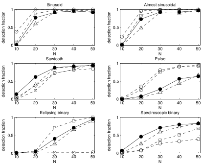
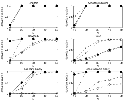
Fig. 2 presents the same test for the case of a high SNR. We fixed the SNR at a value of and repeated the same exercise. In this situation the BKR was again improving over the Hoeffding-test approach, which also meant it performed significantly better than the traditional approaches in the cases of sawtooth-shaped signal and eccentric SB RV curve). However, specifically in those two cases, another trend emerged: the BKR method seemed to have an exceedingly better performance for datasets with very few samples ().
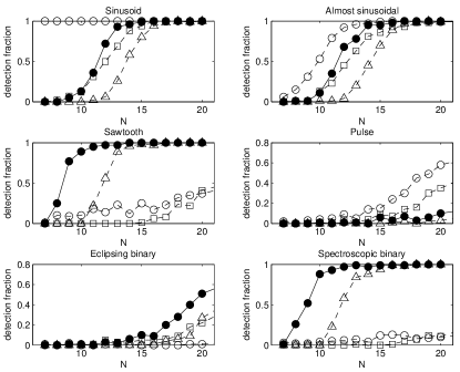
In order to make sure this result was not spurious or even erroneous, we have decided to examine this regime more closely. We repeated the simulations with for a finer grid of , namely, for all from to . Fig. 3 , which focuses on this range, shows the very convincing result of a gradual increase of the performance in most cases. Specifically in the cases of the sawtooth signal and the eccentric SB RV curve, The pace of that increase for the BKR method is much faster than that of the other techniques, including the Hoeffding-test approach. It seemed that already when there were (!) samples, the BKR approach had very good chances to detect the periodicity.
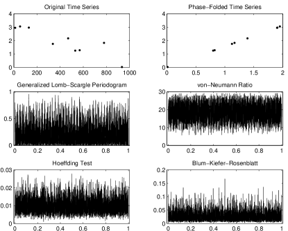
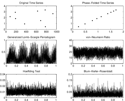
Figs. 4,5 and 6 show selected concrete examples of cases with a sawtooth signal shape and only samples, in which the performance of BKR was definitely superior over the three other techniques we tested. Those cases were indeed the majority of the simulated cases.
4 Real-life test
We set out to test our new technique in a real-life situation that could potentially emphasize its advantages and allow them to materialize. To this end we chose to apply it to short Hipparcos lightcurves. Our sample consisted of Hipparcos targets with at most samples in their Hipparcos Epoch Photometry Annex entry. We considered only samples which were fully accepted by at least one of Hipparcos’ FAST and NDAC consortia (ESA, 1997). In total there were lightcurves meeting those criteria.
We scanned the selected lightcurves for periodicity using the BKR test, on a frequency grid ranging from to (following Koen & Eyer (2002)), with steps of . We searched for targets whose peak in the BKR function was significantly prominent. We therefore used the SDE (Signal Detection Efficiency) statistic originally used by Alcock et al. (2000) and Kovács et al. (2002). We chose to single out targets whose SDE statistic was higher than . Only one target passed this hurdle – HIP 101453 (also known as CH Aql).
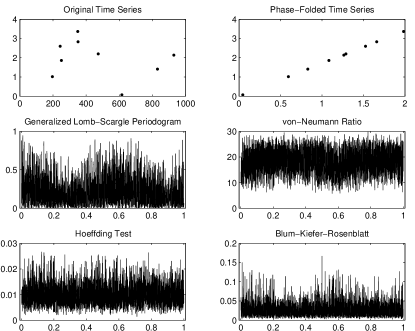
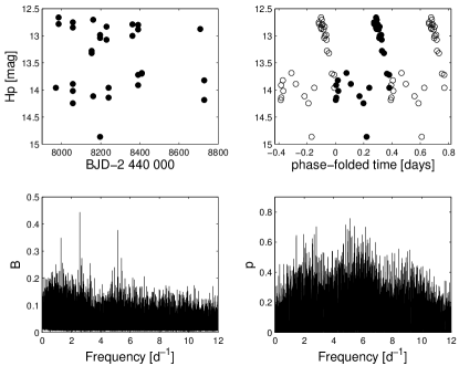
Fig. 7 shows the lightcurve of HIP 101453, as well as its phase folding using the resulting period, the BKR function and the GLS periodogram we calculated for comparison. The prominence of the BKR peak at a frequency of is evident, and indeed the corresponding SDE value is . The phase-folded lightcurve demonstrates an obvious periodicity. On the other hand, The GLS periodogram shows no hint of a statistically significant periodicity detection.
To complete the picture, this star is a known RR-Lyrae star, with a period of d (Samus et al., 2013), which is consistent with our result – d. The Hipparcos catalogue quotes the known period as taken from literature, and adds a comment about the scarcity of the data, which casts doubt about the nature of the periodicity. Therefore, the main catalogue does not quote any period. We show here that by using our new BKR approach, we can assign a high degree of credibility to the periodicity, even with the very scarce Hipparcos data.
5 Discussion
This Letter presents an improvement of the serial Hoeffding-test periodicity metric we have presented in Paper I, based on the Blum-Kiefer-Rosenblatt modification of the original Hoeffding test. This new periodicity metric consistently outperforms the Hoeffding-test metric. On top of it, it seems to perform superbly better in sawtooth-like signal shapes, when the number of samples is very small and the SNR is high. This result is in line with the statement of Blum et al. (1961), that their test is asymptotically equivalent to the Hoeffding test for large samples.
This advantage might prove very important for radial-velocity surveys searching for exoplanets. The detection of high-eccentricity Keplerian RV curves is notoriously difficult when based on a small number of samples (Cumming, 2004). Another situation in which this feature will prove valuable is the detection of RR-Lyrae stars and Cepheids (whose signal shapes are also essentially sawtooth-like shapes) in sparse datasets such as those of Hipparcos and Gaia (Eyer et al., 2012). We have provided in Section 4 a demonstration of this potential using Hipparcos data, specifically for the case of HIP 101453.
We continue our investigation of harnessing the power of non-parametric independence measures for the purpose of detecting periodicity in extreme circumstances of either poor SNR, small sample sizes, or non-sinusoidal signal shapes. In the meanwhile we also apply our newly developed approaches to existing datasets, both for the sake of testing, but also for detecting previously missed periodic variables. To promote further research and testing of this periodicity metric by the community, we make it available online, in the form of a MATLAB function111The URL for downloading a MATLAB code to calculate the BKR periodicity metric is http://www.tau.ac.il/~shayz/BKR.m.
References
- Alcock et al. (2000) Alcock C. et al. 2000, ApJ, 542, 257
- Babu & Feigelson (2006) Babu G. J., Feigelson, E. D. 2006 in Gabriel C., Arviset, C., Ponz D., Enrique S., eds, ASP Conf. Ser. Vol. 351, Astronomical Data Analysis Software and Systems XV. Astron. Soc. Pac., San Francisco, p. 127
- Blum et al. (1961) Blum J. R., Kiefer J., Rosenblatt M. 1961, Ann. Math. Stat., 32, 485
- Clarke (2002) Clarke D. 2002, A&A, 386, 763
- Cramér (1928) Cramér H. 1928, Scand. Actuar. J., 11, 13
- Cumming (2004) Cumming, A. 2004, MNRAS, 354, 1165
- ESA (1997) ESA 1997, The Hipparcos and Tycho Catalogues, ESA SP-1200
- Eyer et al. (2012) Eyer, L. et al. 2012, Ap&SS, 341, 207
- Hoeffding (1948) Hoeffding W. 1948, Ann. Math. Stat., 19, 293
- Koen & Eyer (2002) Koen, C., & Eyer, L. 2002, MNRAS, 331, 45
- Kovács et al. (2002) Kovács G., Zucker S., Mazeh T. 2002, A&A, 391, 369
- Lafler & Kinman (1965) Lafler J., & Kinman, T. D. 1965, ApJS, 11, 216
- Lomb (1976) Lomb N. R. 1976, Ap&SS, 39, 447
- Samus et al. (2013) Samus N. N., Durlevich O. V., Goranskij, V. P., Kazarovets, E. V., Kireeva, N. N., Pastukhova, E. N., Zharova, A.V. 2013, General Catalog of Variable Stars, Vizier online data catalog B/gcvs
- Scargle (1982) Scargle J. D. 1982, ApJ, 263, 835
- von Mises (1928) von Mises R. 1928, Wahrscheinlichkeit, Statistik und Wahrheit, Julius Springer, Vienna
- von Neumann et al. (1941) von Neumann J., Kent R. H., Bellinson H. R., Hart B. I. 1941, Ann. Math. Stat., 12, 153
- Zechmeister & Kürster (2009) Zechmeister, M., & Kürster, M. 2009, A&A, 496, 577
- Zucker (2015) Zucker S. 2015, MNRAS, 449, 2723