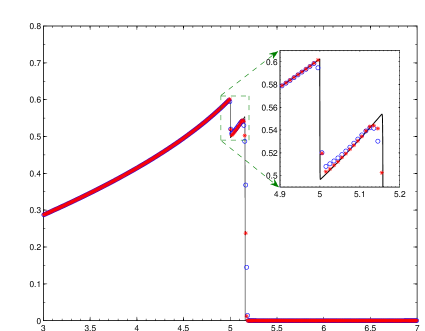
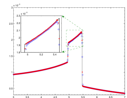
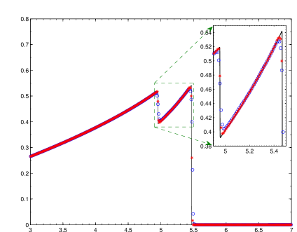
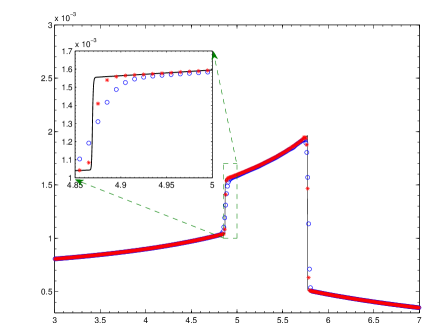
, thanks: Corresponding author. Tel: +86-10-62757018; Fax: +86-10-62751801.

A direct Eulerian GRP scheme for spherically symmetric general relativistic hydrodynamics

Kailiang Wu wukl@pku.edu.cn Huazhong Tang hztang@math.pku.edu.cn HEDPS, CAPT & LMAM, School of Mathematical Sciences, Peking University, Beijing 100871, P.R. China
Abstract

The paper proposes a second-order accurate direct Eulerian generalized Riemann problem (GRP) scheme for the spherically symmetric general relativistic hydrodynamical (RHD) equations and a second-order accurate discretization for the spherically symmetric Einstein (SSE) equations. The former is directly using the Riemann invariants and the Runkine-Hugoniot jump conditions to analytically resolve the left and right nonlinear waves of the local GRP in the Eulerian formulation together with the local change of the metrics to obtain the limiting values of the time derivatives of the conservative variables along the cell interface and the numerical flux for the GRP scheme. While the latter utilizes the energy-momentum tensor obtained in the GRP solver to evaluate the fluid variables in the SSE equations and keeps the continuity of the metrics at the cell interfaces. Several numerical experiments show that the GRP scheme can achieve second-order accuracy and high resolution, and is effective for spherically symmetric general RHD problems.

keywords:
Spherically symmetric general relativistic hydrodynamics; Godunov-type scheme; generalized Riemann problem; Riemann problem; Riemann invariant; Rankine-Hugoniot jump condition.

1 Introduction

Many fields such as high-energy astrophysics etc. may involve flows at speeds close to the speed of light or influenced by large gravitational potentials such that the relativistic effect should be taken into account. Relativistic flows appear in numerous astrophysical phenomena, from stellar to galactic scales, e.g. super-luminal jets, gamma-ray bursts, core collapse super-novae, coalescing neutron stars, formation of black holes and so on.

The governing equations of the relativistic hydrodynamics (RHD) are highly nonlinear so that their analytical treatment is extremely difficult. A primary and powerful approach to understand the physical mechanisms in RHDs is numerical simulations. The pioneering numerical work may date back to the finite difference code by May and White with the artificial viscosity technique for spherically symmetric general RHD equations in the Lagrangian coordinate [20, 21]. Wilson first attempted to numerically solve multi-dimensional RHD equations in the Eulerian coordinate by using the finite difference method with the artificial viscosity technique [33], which was systematically introduced in [34]. Since 1990s, the numerical study of the RHDs began to attract considerable attention, and various modern shock-capturing methods based on exact or approximate Riemann solvers have been developed for the RHD equations, the readers are referred to the early review articles [19, 5] and more recent works on numerical methods for the RHD equations in [35, 36]. Recently, second-order accurate direct Eulerian generalized Riemann problem (GRP) schemes were developed for both 1D and 2D special RHD equations [40, 41] and the third-order accurate extension to the 1D case was also presented in [38].

The GRP scheme, as an analytic high-order accurate extension of the Godunov method, was originally devised for non-relativistic compressible fluid dynamics [1], by utilizing a piecewise linear function to approximate the “initial” data and then analytically resolving a local GRP at each interface to yield numerical flux, see the comprehensive description in [2]. There exist two versions of the original GRP scheme: the Lagrangian and Eulerian. The Eulerian version is always derived by using the Lagrangian framework with a transformation, which is quite delicate, particularly for the sonic case and multi-dimensional application. To avoid those difficulties, second-order accurate direct Eulerian GRP schemes were respectively developed for the shallow water equations [12], the Euler equations [4], and a more general weakly coupled system [3] by directly resolving the local GRPs in the Eulerian formulation via the Riemann invariants and Rankine-Hugoniot jump conditions. A recent comparison of the GRP scheme with the gas-kinetic scheme showed the good performance of the GRP solver for some inviscid flow simulations [13]. Combined with the moving mesh method [29], the adaptive direct Eulerian GRP scheme was developed in [9] with improved resolution as well as accuracy. The accuracy and performance of the adaptive GRP scheme were further studied in [10] in simulating 2D complex wave configurations formulated with the 2D Riemann problems of non-relativistic Euler equations. Recently, the adaptive GRP scheme was also extended to unstructured triangular meshes [16]. The third-order accurate extensions of the direct Eulerian GRP scheme were studied for 1D and 2D non-relativistic Euler equations in [37] and the general 1D hyperbolic balance laws in [25].

The aim of the paper is to develop a second-order accurate direct Eulerian GRP scheme for spherically symmetric general RHD equations. The traditional Godunov-type schemes based on exact or approximate Riemann solvers can be extended to the general RHD equations from the special RHD case through a local change of coordinates in terms of that the spacetime metric is locally Minkowskian [24]. Similar idea can be found in developing the so-called locally inertial Godunov method for spherically symmetric general RHD equations [32]. However, such approach cannot be used to develop the direct Eulerian GRP scheme for the general RHD equations, because it is necessary to resolve the local GRP together with the local change of the metrics taken into account. Moreover, the metrics should be approximately obtained at the cell interface by accurate scheme for the SSE equations to keep the continuity of the approximate metric functions. In short, developing the GRP scheme for the general RHD equations is not trivial and much more technical than the special relativistic case.

The paper is organized as follows. Section 2 introduces the governing equations of general RHDs in spherically symmetric spacetime and corresponding Riemann invariants as well as their total differentials. The second-order accurate direct Eulerian GRP scheme is developed in Section 3. The outline of the scheme is first given in Section 3.1. Then the local GRPs are analytically resolved in Section 3.2, where Sections 3.2.1 and 3.2.2 resolve the rarefaction and shock waves by using the Riemann invariants and the Rankine-Hugoniot jump conditions, respectively, Section 3.2.3 concludes the the limiting values of the time derivatives of the conservative variables at the “initial” discontinuous point along the cell interface for both nonsonic and sonic cases, and Section 3.2.4 discusses the acoustic case. Several numerical experiments are conducted in Section 4 to demonstrate the performance and accuracy of the proposed GRP scheme. Section 5 concludes the paper with several remarks.

2 Governing equations

The general RHD equations [5] consist of the local conservation laws of the current density Jμsuperscript𝐽𝜇J^{\mu} and the stress-energy tensor Tμνsuperscript𝑇𝜇𝜈T^{\mu\nu}

μJμ=0,subscript𝜇superscript𝐽𝜇0\displaystyle\nabla_{\mu}J^{\mu}=0, (2.1)
μTμν=0,subscript𝜇superscript𝑇𝜇𝜈0\displaystyle\nabla_{\mu}T^{\mu\nu}=0, (2.2)

where the indexes μ𝜇\mu and ν𝜈\nu run from 0 to 3, and μsubscript𝜇\nabla_{\mu} stands for the covariant derivative associated with the four-dimensional spacetime metric gμνsubscript𝑔𝜇𝜈g_{\mu\nu}, that is, the proper spacetime distance between any two points in the four-dimensional spacetime can be measured by the line element ds2=gμνdxμdxν𝑑superscript𝑠2subscript𝑔𝜇𝜈𝑑superscript𝑥𝜇𝑑superscript𝑥𝜈ds^{2}=g_{\mu\nu}dx^{\mu}dx^{\nu}. The current density is given by Jμ=ρ0uμsuperscript𝐽𝜇subscript𝜌0superscript𝑢𝜇J^{\mu}=\rho_{0}u^{\mu}, where uμsuperscript𝑢𝜇u^{\mu} represents the fluid four-velocity and ρ0subscript𝜌0\rho_{0} denotes the proper rest-mass density. The stress-energy tensor for an ideal fluid is defined by

Tμν=(ρ+p)uμuν+pgμν,superscript𝑇𝜇𝜈𝜌𝑝superscript𝑢𝜇superscript𝑢𝜈𝑝superscript𝑔𝜇𝜈\displaystyle T^{\mu\nu}=(\rho+p)u^{\mu}u^{\nu}+pg^{\mu\nu},

in which ρ𝜌\rho and p𝑝p denote the rest energy density (including rest-mass) in the fluid frame and the pressure, respectively, and gμλgλν=δνμsuperscript𝑔𝜇𝜆subscript𝑔𝜆𝜈subscriptsuperscript𝛿𝜇𝜈g^{\mu\lambda}g_{\lambda\nu}=\delta^{\mu}_{\nu} with δνμsubscriptsuperscript𝛿𝜇𝜈\delta^{\mu}_{\nu} denoting the Kronecker symbol. The rest energy density ρ𝜌\rho can be expressed in terms of the rest-mass density ρ0subscript𝜌0\rho_{0} and the internal energy e𝑒e as ρ=ρ0(c2+e)𝜌subscript𝜌0superscript𝑐2𝑒\rho=\rho_{0}(c^{2}+e), where c𝑐c denotes the speed of light in vacuum.

An additional equation for the thermodynamical variables, i.e. the so-called equation of state, is needed to close the system (2.1)–(2.2) for a fixed spacetime. This paper focuses on the equation of state describing barotropic fluids

p=p(ρ),𝑝𝑝𝜌p=p(\rho), (2.3)

where p(ρ)𝑝𝜌p(\rho) is a function of ρ𝜌\rho and satisfies

0<dpdρ=p(ρ)<1.0𝑑𝑝𝑑𝜌superscript𝑝𝜌10<\frac{dp}{d\rho}=p^{\prime}(\rho)<1. (2.4)

It is worth noting that the equations (2.2)–(2.5) form a close system if gμνsuperscript𝑔𝜇𝜈g^{\mu\nu} is given. In the general theory, the Einstein gravitational field equations relate the curvature of spacetime to the distribution of mass-energy in the following form

Rμν12gμνR=κTμν,superscript𝑅𝜇𝜈12superscript𝑔𝜇𝜈𝑅𝜅superscript𝑇𝜇𝜈R^{\mu\nu}-\frac{1}{2}g^{\mu\nu}R=\kappa T^{\mu\nu}, (2.5)

where κ=8π𝒢c4𝜅8𝜋𝒢superscript𝑐4\kappa=\frac{8\pi{\cal G}}{c^{4}} is Einstein coupling constant, 𝒢𝒢\cal G is Newton’s gravitational constant, and Rμνsuperscript𝑅𝜇𝜈R^{\mu\nu} and R𝑅R denote the Ricci tensor and the scalar curvature, respectively. For the sake of convenience, units in which the speed of light c𝑐c and Newton’s gravitational constant 𝒢𝒢\cal G are equal to one will be used throughout the paper.

The general RHD system in spherically symmetric spacetime is a simple but good “approximate” model in investigating several astrophysical phenomena, e.g. gamma-ray bursts, spherical accretion onto compact objects, and stellar collapse, etc. Its numerical methods have also received lots of attentions, see e.g. [20, 6, 27, 39, 17, 18, 22, 26, 8, 32, 23]. The spherically symmetric gravitational metrics in standard Schwarzschild coordinates are given by the line element [32]

ds2=B(t,r)dt2+1A(t,r)dr2+r2(dθ2+sin2θdϕ2).𝑑superscript𝑠2𝐵𝑡𝑟𝑑superscript𝑡21𝐴𝑡𝑟𝑑superscript𝑟2superscript𝑟2𝑑superscript𝜃2superscript2𝜃𝑑superscriptitalic-ϕ2ds^{2}=-B(t,r)dt^{2}+\frac{1}{A(t,r)}dr^{2}+r^{2}(d\theta^{2}+\sin^{2}\theta d\phi^{2}). (2.6)

where B(t,r)𝐵𝑡𝑟B(t,r) is called the lapse function, (t,r)𝑡𝑟(t,r) are temporal and radial coordinates, and 𝒙=(x0,x1,x2,x3)=(t,r,θ,ϕ)𝒙superscript𝑥0superscript𝑥1superscript𝑥2superscript𝑥3𝑡𝑟𝜃italic-ϕ\mbox{\boldmath\small$x$}=(x^{0},x^{1},x^{2},x^{3})=(t,r,\theta,\phi) is the spacetime coordinate system. This paper is only concerned with the numerical method for the system (2.2)–(2.5) in spherically symmetric spacetime (2.6). Assume that the spherically symmetric metrics are Lipschitz and the stress-energy tensor is bounded in sup-norm, then the system (2.2)–(2.5) is weakly equivalent to the following system [7]

𝑼t+(AB𝑭(𝑼))r=𝑺(r,A,B,𝑼),𝑼𝑡𝐴𝐵𝑭𝑼𝑟𝑺𝑟𝐴𝐵𝑼\displaystyle\frac{{\partial\mbox{\boldmath\small$U$}}}{{\partial t}}+\frac{\partial\big{(}\sqrt{AB}\mbox{\boldmath\small$F$}(\mbox{\boldmath\small$U$})\big{)}}{{\partial r}}=\mbox{\boldmath\small$S$}(r,A,B,\mbox{\boldmath\small$U$}), (2.7)
Mr=12κr2𝒯00,𝑀𝑟12𝜅superscript𝑟2superscript𝒯00\displaystyle\frac{{\partial M}}{{\partial r}}=\frac{1}{2}\kappa r^{2}{\cal T}^{00}, (2.8)
1BBr=1AAr+κrA𝒯11,1𝐵𝐵𝑟1𝐴𝐴𝑟𝜅𝑟𝐴superscript𝒯11\displaystyle\frac{1}{B}\frac{{\partial B}}{{\partial r}}=\frac{{1-A}}{{Ar}}+\frac{{\kappa r}}{A}{\cal T}^{11}, (2.9)

where

𝑼=(𝒯00,𝒯01)T,𝑭=(𝒯01,𝒯11)T,formulae-sequence𝑼superscriptsuperscript𝒯00superscript𝒯01T𝑭superscriptsuperscript𝒯01superscript𝒯11T\displaystyle\mbox{\boldmath\small$U$}=({\cal T}^{00},{\cal T}^{01})^{\rm T},\quad\mbox{\boldmath\small$F$}=({\cal T}^{01},{\cal T}^{11})^{\rm T},
𝑺=AB(2r𝒯01,2r𝒯11+1A2Ar(𝒯00𝒯11)+κrA(𝒯00𝒯11(𝒯01)2)2pr)T,𝑺𝐴𝐵superscript2𝑟superscript𝒯012𝑟superscript𝒯111𝐴2𝐴𝑟superscript𝒯00superscript𝒯11𝜅𝑟𝐴superscript𝒯00superscript𝒯11superscriptsuperscript𝒯0122𝑝𝑟T\displaystyle\mbox{\boldmath\small$S$}=-\sqrt{AB}\bigg{(}\frac{2}{r}{\cal T}^{01},\frac{2}{r}{\cal T}^{11}+\frac{1-A}{2Ar}({\cal T}^{00}-{\cal T}^{11})+\frac{\kappa r}{A}\big{(}{\cal T}^{00}{\cal T}^{11}-({\cal T}^{01})^{2}\big{)}-\frac{2p}{r}\bigg{)}^{\rm T},

and the mass function M𝑀M is related to A𝐴A by A=12M/r𝐴12𝑀𝑟A=1-2M/r. Here

𝒯00=(ρ+p)W2p,𝒯01=(ρ+p)W2v,𝒯11=(ρv2+p)W2,formulae-sequencesuperscript𝒯00𝜌𝑝superscript𝑊2𝑝formulae-sequencesuperscript𝒯01𝜌𝑝superscript𝑊2𝑣superscript𝒯11𝜌superscript𝑣2𝑝superscript𝑊2{\cal T}^{00}=\left({\rho+p}\right)W^{2}-p,\quad{\cal T}^{01}=\left({\rho+p}\right)W^{2}v,\quad{\cal T}^{11}=\left({\rho v^{2}+p}\right)W^{2},

are the stress-energy tensor in locally flat Minkowski spacetime, related to Tμνsuperscript𝑇𝜇𝜈T^{\mu\nu} by

𝒯00=BT00,𝒯01=BAT01,𝒯11=1AT11,formulae-sequencesuperscript𝒯00𝐵superscript𝑇00formulae-sequencesuperscript𝒯01𝐵𝐴superscript𝑇01superscript𝒯111𝐴superscript𝑇11{\cal T}^{00}=BT^{00},\quad{\cal T}^{01}=\sqrt{\frac{B}{A}}T^{01},\quad{\cal T}^{11}=\frac{1}{A}T^{11},

and W=1/1v2𝑊11superscript𝑣2W=1/\sqrt{1-v^{2}} is the Lorentz factor with the velocity

v:=1ABu1u0.assign𝑣1𝐴𝐵superscript𝑢1superscript𝑢0v:=\frac{1}{\sqrt{AB}}\frac{u^{1}}{u^{0}}.

Eq. (2.8) may be replaced with

Mt=12κr2AB𝒯01,𝑀𝑡12𝜅superscript𝑟2𝐴𝐵superscript𝒯01\displaystyle\frac{{\partial M}}{{\partial t}}=-\frac{1}{2}\kappa r^{2}\sqrt{AB}{\cal T}^{01}, (2.10)

to derive another equivalent system (2.7), (2.9), and (2.10).

The eigenvalues of the Jacobian matrix (AB𝑭)/𝑼𝐴𝐵𝑭𝑼\partial(\sqrt{AB}\mbox{\boldmath\small$F$})/\partial\mbox{\boldmath\small$U$} of (2.7) with (2.3) are

λ=AB(vcs1vcs),λ+=AB(v+cs1+vcs),formulae-sequencesubscript𝜆𝐴𝐵𝑣subscript𝑐𝑠1𝑣subscript𝑐𝑠subscript𝜆𝐴𝐵𝑣subscript𝑐𝑠1𝑣subscript𝑐𝑠\lambda_{-}=\sqrt{AB}\bigg{(}\frac{{v-c_{s}}}{{1-vc_{s}}}\bigg{)},\quad\lambda_{+}=\sqrt{AB}\bigg{(}\frac{{v+c_{s}}}{{1+vc_{s}}}\bigg{)},

where cs=p(ρ)subscript𝑐𝑠superscript𝑝𝜌c_{s}=\sqrt{p^{\prime}(\rho)} denotes the local sound speed. Corresponding right eigenvectors 𝑹±subscript𝑹plus-or-minus\mbox{\boldmath\small$R$}_{\pm}, may be given as follows

𝑹=(1vcsvcs),𝑹+=(1+vcsv+cs),formulae-sequencesubscript𝑹1𝑣subscript𝑐𝑠𝑣subscript𝑐𝑠subscript𝑹1𝑣subscript𝑐𝑠𝑣subscript𝑐𝑠\mbox{\boldmath\small$R$}_{-}=\left(\begin{array}[]{c}1-vc_{s}\\ v-c_{s}\\ \end{array}\right),\quad\mbox{\boldmath\small$R$}_{+}=\left(\begin{array}[]{c}1+vc_{s}\\ v+c_{s}\\ \end{array}\right),

and the inverse of the matrix 𝑹:=(𝑹,𝑹+)assign𝑹subscript𝑹subscript𝑹\mbox{\boldmath\small$R$}:=(\mbox{\boldmath\small$R$}_{-},\mbox{\boldmath\small$R$}_{+}) is

𝑹1=W22cs(v+cs(1+vcs)csv1vcs).superscript𝑹1superscript𝑊22subscript𝑐𝑠𝑣subscript𝑐𝑠1𝑣subscript𝑐𝑠missing-subexpressionmissing-subexpressionmissing-subexpressionmissing-subexpressionmissing-subexpressionmissing-subexpressionmissing-subexpressionmissing-subexpressionmissing-subexpressionmissing-subexpressionmissing-subexpressionmissing-subexpressionmissing-subexpressionmissing-subexpressionmissing-subexpressionmissing-subexpressionmissing-subexpressionmissing-subexpressionsubscript𝑐𝑠𝑣1𝑣subscript𝑐𝑠missing-subexpressionmissing-subexpressionmissing-subexpressionmissing-subexpressionmissing-subexpressionmissing-subexpressionmissing-subexpressionmissing-subexpressionmissing-subexpressionmissing-subexpressionmissing-subexpressionmissing-subexpressionmissing-subexpressionmissing-subexpressionmissing-subexpressionmissing-subexpressionmissing-subexpressionmissing-subexpression\mbox{\boldmath\small$R$}^{-1}=\frac{{W^{2}}}{{2c_{s}}}\left({\begin{array}[]{*{20}c}{v+c_{s}{}}&~{}~{}{-(1+vc_{s})}\\ {c_{s}-v{}}&~{}~{}{1-vc_{s}}\\ \end{array}}\right).

The condition (2.4) implies that λ<λ+subscript𝜆subscript𝜆\lambda_{-}<\lambda_{+}. Thus the system (2.7) is strictly hyperbolic. Moreover, both characteristic fields related to λ±subscript𝜆plus-or-minus\lambda_{\pm} are genuinely nonlinear if and only if the function p(ρ)𝑝𝜌p(\rho) further satisfies [7]

p′′(ρ)>2p(ρ)(1p(ρ))ρ+p(ρ),superscript𝑝′′𝜌2superscript𝑝𝜌1superscript𝑝𝜌𝜌𝑝𝜌{p^{\prime\prime}(\rho)}>-\frac{{2p^{\prime}(\rho)(1-p^{\prime}(\rho))}}{{\rho+p(\rho)}}, (2.11)

which does always hold for

p(ρ)=σ2ρ,σ(0,1).formulae-sequence𝑝𝜌superscript𝜎2𝜌𝜎01p(\rho)=\sigma^{2}\rho,\quad\sigma\in(0,1). (2.12)

The Riemann invariants ψ±subscript𝜓plus-or-minus\psi_{\pm} associated with the characteristic field λ±subscript𝜆plus-or-minus\lambda_{\pm} can be obtained as follows [7]

ψ±=12ln(1+v1v)ρp(ω)ω+p(ω)𝑑ω,subscript𝜓plus-or-minusminus-or-plus121𝑣1𝑣superscript𝜌superscript𝑝𝜔𝜔𝑝𝜔differential-d𝜔\psi_{\pm}=\frac{1}{2}\ln\left({\frac{{1+v}}{{1-v}}}\right)\mp\int^{\rho}{\frac{{\sqrt{p^{\prime}(\omega)}}}{{\omega+p(\omega)}}}d\omega, (2.13)

which will play a pivotal role in resolving the centered rarefaction waves in the direct Eulerian GRP scheme for the RHD equations (2.7).

In the smooth region, by using (2.8) and (2.9), the RHD equations (2.7) can be reformed in the primitive variable vector 𝑽:=(ρ,v)Tassign𝑽superscript𝜌𝑣T\mbox{\boldmath\small$V$}:=(\rho,v)^{\rm T} as follows

𝑽t+𝑱𝑽r=𝑯,𝑽𝑡𝑱𝑽𝑟𝑯\frac{{\partial\mbox{\boldmath\small$V$}}}{{\partial t}}+\mbox{\boldmath\small$J$}\frac{\partial\mbox{\boldmath\small$V$}}{{\partial r}}=\mbox{\boldmath\small$H$},\\ (2.14)

where

𝑱=AB1v2cs2(v(1cs2)ρ+p(1v2)2cs2ρ+pv(1cs2)),𝑱𝐴𝐵1superscript𝑣2superscriptsubscript𝑐𝑠2𝑣1superscriptsubscript𝑐𝑠2𝜌𝑝missing-subexpressionmissing-subexpressionmissing-subexpressionmissing-subexpressionmissing-subexpressionmissing-subexpressionmissing-subexpressionmissing-subexpressionmissing-subexpressionmissing-subexpressionmissing-subexpressionmissing-subexpressionmissing-subexpressionmissing-subexpressionmissing-subexpressionmissing-subexpressionmissing-subexpressionmissing-subexpressionsuperscript1superscript𝑣22superscriptsubscript𝑐𝑠2𝜌𝑝𝑣1superscriptsubscript𝑐𝑠2missing-subexpressionmissing-subexpressionmissing-subexpressionmissing-subexpressionmissing-subexpressionmissing-subexpressionmissing-subexpressionmissing-subexpressionmissing-subexpressionmissing-subexpressionmissing-subexpressionmissing-subexpressionmissing-subexpressionmissing-subexpressionmissing-subexpressionmissing-subexpressionmissing-subexpressionmissing-subexpression\displaystyle\mbox{\boldmath\small$J$}=\frac{\sqrt{AB}}{{1-v^{2}c_{s}^{2}}}\left({\begin{array}[]{*{20}c}{v(1-c_{s}^{2})}&{\rho+p}\\ {\frac{{(1-v^{2})^{2}c_{s}^{2}}}{{\rho+p}}}&{v(1-c_{s}^{2})}\\ \end{array}}\right),
𝑯=(H1,H2)T=ABr(1v2cs2)(2v(ρ+p)(1κr2(ρ+p)4A)(1v2)(2v2cs2+(1A)(1v2cs2)2A+κr2(p+ρv2cs2)2A)).𝑯superscriptsubscript𝐻1subscript𝐻2T𝐴𝐵𝑟1superscript𝑣2superscriptsubscript𝑐𝑠22𝑣𝜌𝑝1𝜅superscript𝑟2𝜌𝑝4𝐴1superscript𝑣22superscript𝑣2superscriptsubscript𝑐𝑠21𝐴1superscript𝑣2superscriptsubscript𝑐𝑠22𝐴𝜅superscript𝑟2𝑝𝜌superscript𝑣2superscriptsubscript𝑐𝑠22𝐴\displaystyle\mbox{\boldmath\small$H$}=(H_{1},H_{2})^{\rm T}=-\frac{{\sqrt{AB}}}{{r(1-v^{2}c_{s}^{2})}}\left(\begin{array}[]{c}2v(\rho+p)\left({1-\frac{{\kappa r^{2}(\rho+p)}}{4A}}\right)\\ (1-v^{2})\left({-2v^{2}c_{s}^{2}+\frac{{(1-A)(1-v^{2}c_{s}^{2})}}{{2A}}+\frac{{\kappa r^{2}(p+\rho v^{2}c_{s}^{2})}}{2A}}\right)\\ \end{array}\right).

By using (2.14), one can derive the following differential relations of the Riemann invariants

D±ψDtsubscript𝐷plus-or-minussubscript𝜓minus-or-plus𝐷𝑡\displaystyle\frac{{D_{\pm}\psi_{\mp}}}{{Dt}} =11v2D±vDt±csρ+pD±ρDt=11v2H2±csρ+pH1=:s,\displaystyle=\frac{1}{{1-v^{2}}}\frac{{D_{\pm}v}}{{Dt}}\pm\frac{{c_{s}}}{{\rho+p}}\frac{{D_{\pm}\rho}}{{Dt}}=\frac{1}{{1-v^{2}}}H_{2}\pm\frac{{c_{s}}}{{\rho+p}}H_{1}=:s_{\mp}, (2.15)

where

D±Dt:=t+λ±r,assignsubscript𝐷plus-or-minus𝐷𝑡𝑡subscript𝜆plus-or-minus𝑟\frac{{D_{\pm}}}{{Dt}}:=\frac{\partial}{\partial t}+\lambda_{\pm}\frac{\partial}{\partial r},

denote the total derivative operators along the characteristic curves drdt=λ±𝑑𝑟𝑑𝑡subscript𝜆plus-or-minus\frac{dr}{dt}=\lambda_{\pm}.

3 Numerical scheme

3.1 The outline of the GRP scheme

This subsection gives the outline of the GRP scheme. For the sake of simplicity, the equally spaced grid points {rj+12=(j+12)Δr}subscript𝑟𝑗12𝑗12Δ𝑟\left\{r_{j+\frac{1}{2}}=\left(j+\frac{1}{2}\right)\Delta r\right\} are used for the spatial domain ΩΩ\Omega and the cell is denoted by Ij=[rj12,rj+12]subscript𝐼𝑗subscript𝑟𝑗12subscript𝑟𝑗12I_{j}=[r_{j-\frac{1}{2}},r_{j+\frac{1}{2}}], j+𝑗superscriptj\in\mathbb{Z}^{+}. The time domain [0,T]0𝑇[0,T] is also divided into the (non-uniform) grid {t0=0,tn+1=tn+Δtn,n0}formulae-sequencesubscript𝑡00formulae-sequencesubscript𝑡𝑛1subscript𝑡𝑛Δsubscript𝑡𝑛𝑛0\{t_{0}=0,t_{n+1}=t_{n}+\Delta t_{n},n\geq 0\} with the time step size ΔtnΔsubscript𝑡𝑛\Delta t_{n} determined by

Δtn=CcflΔrmaxj{|λ(𝑼jn,Ajn,Bjn)|,|λ+(𝑼jn,Ajn,Bjn)|},Δsubscript𝑡𝑛subscript𝐶𝑐𝑓𝑙Δ𝑟subscript𝑗subscript𝜆superscriptsubscript𝑼𝑗𝑛superscriptsubscript𝐴𝑗𝑛superscriptsubscript𝐵𝑗𝑛subscript𝜆superscriptsubscript𝑼𝑗𝑛superscriptsubscript𝐴𝑗𝑛superscriptsubscript𝐵𝑗𝑛\Delta t_{n}=C_{cfl}\frac{\Delta r}{\max\limits_{j}\left\{|\lambda_{-}({\mbox{\boldmath\small$U$}}_{j}^{n},A_{j}^{n},B_{j}^{n})|,|\lambda_{+}({\mbox{\boldmath\small$U$}}_{j}^{n},A_{j}^{n},B_{j}^{n})|\right\}},

where 𝑼jnsuperscriptsubscript𝑼𝑗𝑛{\mbox{\boldmath\small$U$}}_{j}^{n}, Ajnsuperscriptsubscript𝐴𝑗𝑛A_{j}^{n}, and Bjnsuperscriptsubscript𝐵𝑗𝑛B_{j}^{n} approximate the values of 𝑼(t,r)𝑼𝑡𝑟\mbox{\boldmath\small$U$}(t,r), A(t,r)𝐴𝑡𝑟A(t,r) and B(t,r)𝐵𝑡𝑟B(t,r) at the point (tn,rj)subscript𝑡𝑛subscript𝑟𝑗(t_{n},r_{j}), respectively, and Ccflsubscript𝐶𝑐𝑓𝑙C_{cfl} is the CFL number.

Assume that the “initial” data at time t=tn𝑡subscript𝑡𝑛t=t_{n} are piecewise linear functions as follows

{𝑼h(tn,r)=𝑼jn+𝝈jn(rrj)=:𝑼jn(r),(Ah(tn,r)Bh(tn,r))=rj+12rΔr(Aj12nBj12n)+rrj12Δr(Aj+12nBj+12n),\left\{\begin{array}[]{l}\mbox{\boldmath\small$U$}_{h}(t_{n},r)=\mbox{\boldmath\small$U$}_{j}^{n}+\mbox{\boldmath\small$\sigma$}_{j}^{n}(r-r_{j})=:\mbox{\boldmath\small$U$}^{n}_{j}(r),\\[8.53581pt] \left(\begin{array}[]{c}A_{h}(t_{n},r)\\ B_{h}(t_{n},r)\\ \end{array}\right)=\displaystyle{\frac{{r_{j+\frac{1}{2}}-r}}{{\Delta r}}}\left(\begin{array}[]{c}A_{j-\frac{1}{2}}^{n}\\ B_{j-\frac{1}{2}}^{n}\\ \end{array}\right)+\displaystyle{\frac{r-r_{j-\frac{1}{2}}}{\Delta r}}\left(\begin{array}[]{c}A_{j+\frac{1}{2}}^{n}\\ B_{j+\frac{1}{2}}^{n}\\ \end{array}\right),\end{array}\right. (3.1)

for rIj𝑟subscript𝐼𝑗r\in I_{j}, where Ah(tn,r)subscript𝐴subscript𝑡𝑛𝑟A_{h}(t_{n},r) and Bh(tn,r)subscript𝐵subscript𝑡𝑛𝑟B_{h}(t_{n},r) are continuous at cell interfaces rj±12subscript𝑟plus-or-minus𝑗12r_{j\pm\frac{1}{2}}.

Step I. Evaluate the point values 𝑼j+12n+12superscriptsubscript𝑼𝑗12𝑛12\mbox{\boldmath\small$U$}_{j+\frac{1}{2}}^{n+\frac{1}{2}} approximating 𝑼(tn+12,rj+12)𝑼subscript𝑡𝑛12subscript𝑟𝑗12\mbox{\boldmath\small$U$}(t_{n+\frac{1}{2}},r_{j+\frac{1}{2}}) by

𝑼j+12n+12=𝑼j+12RP,n+Δtn2(𝑼t)j+12GRP,n,superscriptsubscript𝑼𝑗12𝑛12superscriptsubscript𝑼𝑗12RP𝑛Δsubscript𝑡𝑛2superscriptsubscript𝑼𝑡𝑗12GRP𝑛\mbox{\boldmath\small$U$}_{j+\frac{1}{2}}^{n+\frac{1}{2}}=\mbox{\boldmath\small$U$}_{j+\frac{1}{2}}^{\mbox{\tiny RP},n}+\frac{{\Delta t_{n}}}{2}\left({\frac{{\partial\mbox{\boldmath\small$U$}}}{{\partial t}}}\right)_{j+\frac{1}{2}}^{\mbox{\tiny GRP},n}, (3.2)

where 𝑼j+12RP,nsuperscriptsubscript𝑼𝑗12RP𝑛\mbox{\boldmath\small$U$}_{j+\frac{1}{2}}^{\mbox{\tiny RP},n} is the values at r=rj+12𝑟subscript𝑟𝑗12r=r_{j+\frac{1}{2}} of the solutions to the following Riemann problem of the homogeneous hyperbolic conservation laws

{𝑼t+Aj+12nBj+12n𝑭(𝑼)r=0,r>0,t>tn,𝑼(tn,r)={𝑼j+12,Ln:=𝑼h(tn,rj+120),r<rj+12,𝑼j+12,Rn:=𝑼h(tn,rj+12+0),r>rj+12,casesformulae-sequence𝑼𝑡superscriptsubscript𝐴𝑗12𝑛superscriptsubscript𝐵𝑗12𝑛𝑭𝑼𝑟0formulae-sequence𝑟0𝑡subscript𝑡𝑛otherwise𝑼subscript𝑡𝑛𝑟casesassignsuperscriptsubscript𝑼𝑗12𝐿𝑛subscript𝑼subscript𝑡𝑛subscript𝑟𝑗120𝑟subscript𝑟𝑗12assignsuperscriptsubscript𝑼𝑗12𝑅𝑛subscript𝑼subscript𝑡𝑛subscript𝑟𝑗120𝑟subscript𝑟𝑗12otherwise\begin{cases}\displaystyle{\frac{{\partial\mbox{\boldmath\small$U$}}}{{\partial t}}}+\sqrt{A_{j+\frac{1}{2}}^{n}B_{j+\frac{1}{2}}^{n}}\displaystyle{\frac{{\partial\mbox{\boldmath\small$F$}(\mbox{\boldmath\small$U$})}}{{\partial r}}}=0,\qquad r>0,~{}t>t_{n},\\[8.53581pt] \mbox{\boldmath\small$U$}(t_{n},r)=\begin{cases}\mbox{\boldmath\small$U$}_{j+\frac{1}{2},L}^{n}:=\mbox{\boldmath\small$U$}_{h}(t_{n},r_{j+\frac{1}{2}}-0),&r<r_{j+\frac{1}{2}},\\ \mbox{\boldmath\small$U$}_{j+\frac{1}{2},R}^{n}:=\mbox{\boldmath\small$U$}_{h}(t_{n},r_{j+\frac{1}{2}}+0),&r>r_{j+\frac{1}{2}},\end{cases}\end{cases}

and (𝑼/t)j+12GRP,nsuperscriptsubscript𝑼𝑡𝑗12GRP𝑛\left(\partial\mbox{\boldmath\small$U$}/\partial t\right)_{j+\frac{1}{2}}^{\mbox{\tiny GRP},n} is analytically derived by a second order accurate resolution of the local generalized Riemann problem (GRP) at each point (tn,rj+12)subscript𝑡𝑛subscript𝑟𝑗12(t_{n},r_{j+\frac{1}{2}}), i.e.

{Eqs. (2.7),r>0,t>tn,𝑼(tn,r)={𝑼jn(r),r<rj+12,𝑼j+1n(r),r>rj+12.casesformulae-sequenceEqs. (2.7)𝑟0𝑡subscript𝑡𝑛otherwise𝑼subscript𝑡𝑛𝑟casessubscriptsuperscript𝑼𝑛𝑗𝑟𝑟subscript𝑟𝑗12subscriptsuperscript𝑼𝑛𝑗1𝑟𝑟subscript𝑟𝑗12otherwise\begin{cases}\mbox{Eqs. \eqref{eq:RHD_1}},\qquad r>0,~{}t>t_{n},\\[5.69054pt] \mbox{\boldmath\small$U$}(t_{n},r)=\begin{cases}\mbox{\boldmath\small$U$}^{n}_{j}(r),&r<r_{j+\frac{1}{2}},\\ \mbox{\boldmath\small$U$}^{n}_{j+1}(r),&r>r_{j+\frac{1}{2}}.\end{cases}\end{cases} (3.3)

The calculation of (𝑼/t)j+12GRP,nsuperscriptsubscript𝑼𝑡𝑗12GRP𝑛\left(\partial\mbox{\boldmath\small$U$}/\partial t\right)_{j+\frac{1}{2}}^{\mbox{\tiny GRP},n} is one of the key elements in the GRP scheme and will be given in Section 3.2.

Step II. Calculate the point values Aj+12n+12superscriptsubscript𝐴𝑗12𝑛12A_{j+\frac{1}{2}}^{n+\frac{1}{2}} and Bj+12n+12superscriptsubscript𝐵𝑗12𝑛12B_{j+\frac{1}{2}}^{n+\frac{1}{2}}, which are approximation of A(tn+12,rj+12)𝐴subscript𝑡𝑛12subscript𝑟𝑗12A(t_{n+\frac{1}{2}},r_{j+\frac{1}{2}}) and B(tn+12,rj+12)𝐵subscript𝑡𝑛12subscript𝑟𝑗12B(t_{n+\frac{1}{2}},r_{j+\frac{1}{2}}), respectively, by

Mj+12n+12=Mj+12n+Δtn2(Mt)j+12n=Mj+12nΔtn4κrj+122Aj+12nBj+12n𝒯01(𝑼j+12RP,n),superscriptsubscript𝑀𝑗12𝑛12superscriptsubscript𝑀𝑗12𝑛Δsubscript𝑡𝑛2superscriptsubscript𝑀𝑡𝑗12𝑛superscriptsubscript𝑀𝑗12𝑛Δsubscript𝑡𝑛4𝜅superscriptsubscript𝑟𝑗122superscriptsubscript𝐴𝑗12𝑛superscriptsubscript𝐵𝑗12𝑛superscript𝒯01superscriptsubscript𝑼𝑗12RP𝑛\displaystyle M_{j+\frac{1}{2}}^{n+\frac{1}{2}}=M_{j+\frac{1}{2}}^{n}+\frac{{\Delta t_{n}}}{2}\left({\frac{{\partial M}}{{\partial t}}}\right)_{j+\frac{1}{2}}^{n}=M_{j+\frac{1}{2}}^{n}-\frac{{\Delta t_{n}}}{4}\kappa r_{j+\frac{1}{2}}^{2}\sqrt{A_{j+\frac{1}{2}}^{n}B_{j+\frac{1}{2}}^{n}}{\cal T}^{01}\left({\mbox{\boldmath\small$U$}_{j+\frac{1}{2}}^{\mbox{\tiny RP},n}}\right),
Aj+12n+12=12Mj+12n+12/rj+12,superscriptsubscript𝐴𝑗12𝑛1212superscriptsubscript𝑀𝑗12𝑛12subscript𝑟𝑗12\displaystyle A_{j+\frac{1}{2}}^{n+\frac{1}{2}}=1-2M_{j+\frac{1}{2}}^{n+\frac{1}{2}}/r_{j+\frac{1}{2}},
lnBj+12n+12=lnBj12n+12+Δr2(1Aj12n+12Aj12n+12rj12+κrj12Aj12n+12𝒯11(𝑼j12n+12)+1Aj+12n+12Aj+12n+12rj+12+κrj+12Aj+12n+12𝒯11(𝑼j+12n+12)).superscriptsubscript𝐵𝑗12𝑛12superscriptsubscript𝐵𝑗12𝑛12Δ𝑟21superscriptsubscript𝐴𝑗12𝑛12superscriptsubscript𝐴𝑗12𝑛12subscript𝑟𝑗12𝜅subscript𝑟𝑗12superscriptsubscript𝐴𝑗12𝑛12superscript𝒯11superscriptsubscript𝑼𝑗12𝑛121superscriptsubscript𝐴𝑗12𝑛12superscriptsubscript𝐴𝑗12𝑛12subscript𝑟𝑗12𝜅subscript𝑟𝑗12superscriptsubscript𝐴𝑗12𝑛12superscript𝒯11superscriptsubscript𝑼𝑗12𝑛12\displaystyle\ln B_{j+\frac{1}{2}}^{n+\frac{1}{2}}=\ln B_{j-\frac{1}{2}}^{n+\frac{1}{2}}+\frac{{\Delta r}}{2}\left({\frac{{1-A_{j-\frac{1}{2}}^{n+\frac{1}{2}}}}{{A_{j-\frac{1}{2}}^{n+\frac{1}{2}}r_{j-\frac{1}{2}}}}+\frac{{\kappa r_{j-\frac{1}{2}}}}{{A_{j-\frac{1}{2}}^{n+\frac{1}{2}}}}{\cal T}^{11}\left({\mbox{\boldmath\small$U$}_{j-\frac{1}{2}}^{n+\frac{1}{2}}}\right)+\frac{{1-A_{j+\frac{1}{2}}^{n+\frac{1}{2}}}}{{A_{j+\frac{1}{2}}^{n+\frac{1}{2}}r_{j+\frac{1}{2}}}}+\frac{{\kappa r_{j+\frac{1}{2}}}}{{A_{j+\frac{1}{2}}^{n+\frac{1}{2}}}}{\cal T}^{11}\left({\mbox{\boldmath\small$U$}_{j+\frac{1}{2}}^{n+\frac{1}{2}}}\right)}\right).

Step III. Approximately evolve the solution vector 𝑼𝑼U at time tn+1subscript𝑡𝑛1t_{n+1} of (2.7) by a second-order accurate Godunov-type scheme

𝑼jn+1=superscriptsubscript𝑼𝑗𝑛1absent\displaystyle\mbox{\boldmath\small$U$}_{j}^{n+1}= 𝑼jnΔtnΔr(Aj+12n+12Bj+12n+12𝑭(𝑼j+12n+12)Aj12n+12Bj12n+12𝑭(𝑼j12n+12))superscriptsubscript𝑼𝑗𝑛Δsubscript𝑡𝑛Δ𝑟superscriptsubscript𝐴𝑗12𝑛12superscriptsubscript𝐵𝑗12𝑛12𝑭superscriptsubscript𝑼𝑗12𝑛12superscriptsubscript𝐴𝑗12𝑛12superscriptsubscript𝐵𝑗12𝑛12𝑭superscriptsubscript𝑼𝑗12𝑛12\displaystyle\mbox{\boldmath\small$U$}_{j}^{n}-\displaystyle{\frac{{\Delta t_{n}}}{{\Delta r}}}\left({\sqrt{A_{j+\frac{1}{2}}^{n+\frac{1}{2}}B_{j+\frac{1}{2}}^{n+\frac{1}{2}}}\mbox{\boldmath\small$F$}\left({\mbox{\boldmath\small$U$}_{j+\frac{1}{2}}^{n+\frac{1}{2}}}\right)-\sqrt{A_{j-\frac{1}{2}}^{n+\frac{1}{2}}B_{j-\frac{1}{2}}^{n+\frac{1}{2}}}\mbox{\boldmath\small$F$}\left({\mbox{\boldmath\small$U$}_{j-\frac{1}{2}}^{n+\frac{1}{2}}}\right)}\right)
+Δtn2(𝑺(rj12,Aj12n+12,Bj12n+12,𝑼j12n+12)+𝑺(rj+12,Aj+12n+12,Bj+12n+12,𝑼j+12n+12)).Δsubscript𝑡𝑛2𝑺subscript𝑟𝑗12superscriptsubscript𝐴𝑗12𝑛12superscriptsubscript𝐵𝑗12𝑛12superscriptsubscript𝑼𝑗12𝑛12𝑺subscript𝑟𝑗12superscriptsubscript𝐴𝑗12𝑛12superscriptsubscript𝐵𝑗12𝑛12superscriptsubscript𝑼𝑗12𝑛12\displaystyle+\displaystyle{\frac{{\Delta t_{n}}}{2}}\bigg{(}{\mbox{\boldmath\small$S$}\left({r_{j-\frac{1}{2}},A_{j-\frac{1}{2}}^{n+\frac{1}{2}},B_{j-\frac{1}{2}}^{n+\frac{1}{2}},\mbox{\boldmath\small$U$}_{j-\frac{1}{2}}^{n+\frac{1}{2}}}\right)+\mbox{\boldmath\small$S$}\left({r_{j+\frac{1}{2}},A_{j+\frac{1}{2}}^{n+\frac{1}{2}},B_{j+\frac{1}{2}}^{n+\frac{1}{2}},\mbox{\boldmath\small$U$}_{j+\frac{1}{2}}^{n+\frac{1}{2}}}\right)}\bigg{)}. (3.4)

Step V. Calculate Aj+12n+1superscriptsubscript𝐴𝑗12𝑛1A_{j+\frac{1}{2}}^{n+1} and Bj+12n+1superscriptsubscript𝐵𝑗12𝑛1B_{j+\frac{1}{2}}^{n+1} by

Mj+12n+1=Mj12n+1+Δr2κrj2𝒯00(𝑼jn+1),Aj+12n+1=12Mj+12n+1/rj+12,formulae-sequencesuperscriptsubscript𝑀𝑗12𝑛1superscriptsubscript𝑀𝑗12𝑛1Δ𝑟2𝜅superscriptsubscript𝑟𝑗2superscript𝒯00superscriptsubscript𝑼𝑗𝑛1superscriptsubscript𝐴𝑗12𝑛112superscriptsubscript𝑀𝑗12𝑛1subscript𝑟𝑗12\displaystyle M_{j+\frac{1}{2}}^{n+1}=M_{j-\frac{1}{2}}^{n+1}+\frac{{\Delta r}}{2}\kappa r_{j}^{2}{\cal T}^{00}\left({\mbox{\boldmath\small$U$}_{j}^{n+1}}\right),\quad A_{j+\frac{1}{2}}^{n+1}=1-2M_{j+\frac{1}{2}}^{n+1}/r_{j+\frac{1}{2}},
lnBj+12n+1=lnBj12n+1+Δr(1Ajn+1Ajn+1rj+κrjAjn+1𝒯11(𝑼jn+1)),Ajn+1:=12(Aj12n+1+Aj+12n+1).formulae-sequencesuperscriptsubscript𝐵𝑗12𝑛1superscriptsubscript𝐵𝑗12𝑛1Δ𝑟1superscriptsubscript𝐴𝑗𝑛1superscriptsubscript𝐴𝑗𝑛1subscript𝑟𝑗𝜅subscript𝑟𝑗superscriptsubscript𝐴𝑗𝑛1superscript𝒯11superscriptsubscript𝑼𝑗𝑛1assignsuperscriptsubscript𝐴𝑗𝑛112superscriptsubscript𝐴𝑗12𝑛1superscriptsubscript𝐴𝑗12𝑛1\displaystyle\ln B_{j+\frac{1}{2}}^{n+1}=\ln B_{j-\frac{1}{2}}^{n+1}+{\Delta r}\left(\frac{1-A_{j}^{n+1}}{A_{j}^{n+1}r_{j}}+\frac{\kappa r_{j}}{A_{j}^{n+1}}{\cal T}^{11}\left(\mbox{\boldmath\small$U$}_{j}^{n+1}\right)\right),\quad A_{j}^{n+1}:=\frac{1}{2}\big{(}A_{j-\frac{1}{2}}^{n+1}+A_{j+\frac{1}{2}}^{n+1}\big{)}.

Step IV. Update the slope 𝝈jn+1superscriptsubscript𝝈𝑗𝑛1\mbox{\boldmath\small$\sigma$}_{j}^{n+1} component-wisely in the local characteristic variables by

𝝈jn+1=𝑹jminmod(θΔr𝑹j1(𝑼jn+1𝑼j1n+1),𝑹j1𝝈jn+1,,θΔr𝑹j1(𝑼j+1n+1𝑼jn+1)),superscriptsubscript𝝈𝑗𝑛1subscript𝑹𝑗minmod𝜃Δ𝑟superscriptsubscript𝑹𝑗1superscriptsubscript𝑼𝑗𝑛1superscriptsubscript𝑼𝑗1𝑛1superscriptsubscript𝑹𝑗1superscriptsubscript𝝈𝑗𝑛1𝜃Δ𝑟superscriptsubscript𝑹𝑗1superscriptsubscript𝑼𝑗1𝑛1superscriptsubscript𝑼𝑗𝑛1\mbox{\boldmath\small$\sigma$}_{j}^{n+1}=\mbox{\boldmath\small$R$}_{j}{\rm minmod}\left(\frac{\theta}{\Delta r}\mbox{\boldmath\small$R$}_{j}^{-1}\left(\mbox{\boldmath\small$U$}_{j}^{n+1}-\mbox{\boldmath\small$U$}_{j-1}^{n+1}\right),\mbox{\boldmath\small$R$}_{j}^{-1}\mbox{\boldmath\small$\sigma$}_{j}^{n+1,-},\frac{\theta}{\Delta r}\mbox{\boldmath\small$R$}_{j}^{-1}\left(\mbox{\boldmath\small$U$}_{j+1}^{n+1}-\mbox{\boldmath\small$U$}_{j}^{n+1}\right)\right), (3.5)

where 𝑹j:=𝑹(𝑼jn+1)assignsubscript𝑹𝑗𝑹superscriptsubscript𝑼𝑗𝑛1\mbox{\boldmath\small$R$}_{j}:=\mbox{\boldmath\small$R$}(\mbox{\boldmath\small$U$}_{j}^{n+1}), the parameter θ[1,2)𝜃12\theta\in[1,2), and

𝝈jn+1,=1Δr(𝑼j+12n+1,𝑼j12n+1,),𝑼j+12n+1,=𝑼j+12RP,n+Δtn(𝑼t)j+12GRP,n.formulae-sequencesuperscriptsubscript𝝈𝑗𝑛11Δ𝑟superscriptsubscript𝑼𝑗12𝑛1superscriptsubscript𝑼𝑗12𝑛1superscriptsubscript𝑼𝑗12𝑛1superscriptsubscript𝑼𝑗12RP𝑛Δsubscript𝑡𝑛superscriptsubscript𝑼𝑡𝑗12GRP𝑛\mbox{\boldmath\small$\sigma$}_{j}^{n+1,-}=\frac{1}{{\Delta r}}\left({\mbox{\boldmath\small$U$}_{j+\frac{1}{2}}^{n+1,-}-\mbox{\boldmath\small$U$}_{j-\frac{1}{2}}^{n+1,-}}\right),\quad\mbox{\boldmath\small$U$}_{j+\frac{1}{2}}^{n+1,-}=\mbox{\boldmath\small$U$}_{j+\frac{1}{2}}^{\mbox{\tiny RP},n}+\Delta t_{n}\left({\frac{{\partial\mbox{\boldmath\small$U$}}}{{\partial t}}}\right)_{j+\frac{1}{2}}^{\mbox{\tiny GRP},n}.

The paper does not pay much attention to the treatment of singularity in the source 𝑺𝑺S of (2.7) and the imposition of boundary conditions at the symmetric center r=0𝑟0r=0 for the GRP scheme, the readers are referred to [14] for the details.

3.2 Resolution of generalized Riemann problem

This subsection resolves the GRP (3.3) in order to get (𝑼/t)j+12GRP,nsuperscriptsubscript𝑼𝑡𝑗12GRP𝑛\left(\partial\mbox{\boldmath\small$U$}/\partial t\right)_{j+\frac{1}{2}}^{\mbox{\tiny GRP},n} in (3.2). For the sake of convenience, the subscript j𝑗j and the superscript n𝑛n will be ignored and the local GRP (3.3) is transformed with a linear coordinate transformation to the “non-local” GRP for (2.7) with the initial data

𝑼(0,r)={𝑼L+(rr0)𝑼L,r<r0,𝑼R+(rr0)𝑼R,r>r0,𝑼0𝑟casessubscript𝑼𝐿𝑟subscript𝑟0subscriptsuperscript𝑼𝐿𝑟subscript𝑟0subscript𝑼𝑅𝑟subscript𝑟0subscriptsuperscript𝑼𝑅𝑟subscript𝑟0\mbox{\boldmath\small$U$}(0,r)=\begin{cases}\mbox{\boldmath\small$U$}_{L}+(r-r_{0})\mbox{\boldmath\small$U$}^{\prime}_{L},\ \ &r<r_{0},\\[8.53581pt] \mbox{\boldmath\small$U$}_{R}+(r-r_{0})\mbox{\boldmath\small$U$}^{\prime}_{R},&r>r_{0},\end{cases} (3.6)

where 𝑼L,𝑼R,𝑼Lsubscript𝑼𝐿subscript𝑼𝑅subscriptsuperscript𝑼𝐿\mbox{\boldmath\small$U$}_{L},\mbox{\boldmath\small$U$}_{R},\mbox{\boldmath\small$U$}^{\prime}_{L} and 𝑼Rsubscriptsuperscript𝑼𝑅\mbox{\boldmath\small$U$}^{\prime}_{R} are corresponding constant vectors. The notations 𝑼j+1/2RP,nsuperscriptsubscript𝑼𝑗12RP𝑛\mbox{\boldmath\small$U$}_{j+1/2}^{\mbox{\tiny RP},n} and (𝑼t)j+1/2GRP,nsuperscriptsubscriptsubscript𝑼𝑡𝑗12GRP𝑛\left(\mbox{\boldmath\small$U$}_{t}\right)_{j+1/2}^{\mbox{\tiny GRP},n} will also be simply replaced with 𝑼subscript𝑼\mbox{\boldmath\small$U$}_{*} and (𝑼t)subscriptsubscript𝑼𝑡\left(\mbox{\boldmath\small$U$}_{t}\right)_{*}, respectively, which also denote the limiting states at r=r0𝑟subscript𝑟0r=r_{0}, as t0+𝑡superscript0t\rightarrow 0^{+}.

Since both A𝐴A and B𝐵B are locally Lipschitz continuous, the initial structure of the solution 𝑼GRP(t,r)superscript𝑼GRP𝑡𝑟\mbox{\boldmath\small$U$}^{\mbox{\tiny GRP}}(t,r) to the GRP for (2.7) with (3.6) may be determined by the solution 𝑼RP(t,r)=𝝎((rr0)/t;𝑼L,𝑼R)superscript𝑼RP𝑡𝑟𝝎𝑟subscript𝑟0𝑡subscript𝑼𝐿subscript𝑼𝑅\mbox{\boldmath\small$U$}^{\mbox{\tiny RP}}(t,r)=\mbox{\boldmath\small$\omega$}((r-r_{0})/t;\mbox{\boldmath\small$U$}_{L},\mbox{\boldmath\small$U$}_{R}) of the associated (classical) Riemann problem (RP) [1, 15]

{𝑼t+AB𝑭(𝑼)r=0,t>0,𝑼(0,r)={𝑼L,r<r0,𝑼R,r>r0,casesformulae-sequence𝑼𝑡subscript𝐴subscript𝐵𝑭𝑼𝑟0𝑡0otherwise𝑼0𝑟casessubscript𝑼𝐿𝑟subscript𝑟0subscript𝑼𝑅𝑟subscript𝑟0otherwise\begin{cases}\displaystyle{\frac{{\partial\mbox{\boldmath\small$U$}}}{{\partial t}}}+\sqrt{A_{*}B_{*}}\displaystyle{\frac{{\partial\mbox{\boldmath\small$F$}(\mbox{\boldmath\small$U$})}}{{\partial r}}}=0,\qquad t>0,\\[8.53581pt] \mbox{\boldmath\small$U$}(0,r)=\begin{cases}\mbox{\boldmath\small$U$}_{L},\ \ &r<r_{0},\\[2.84526pt] \mbox{\boldmath\small$U$}_{R},&r>r_{0},\end{cases}\end{cases} (3.7)

and

limt0+𝑼GRP(t,tλ+r0)=𝝎(λ;𝑼L,𝑼R),rr0=tλ.formulae-sequencesubscript𝑡superscript0superscript𝑼GRP𝑡𝑡𝜆subscript𝑟0𝝎𝜆subscript𝑼𝐿subscript𝑼𝑅𝑟subscript𝑟0𝑡𝜆\lim_{t\rightarrow 0^{+}}\mbox{\boldmath\small$U$}^{\mbox{\tiny GRP}}(t,t\lambda+r_{0})=\mbox{\boldmath\small$\omega$}(\lambda;\mbox{\boldmath\small$U$}_{L},\mbox{\boldmath\small$U$}_{R}),\quad r-r_{0}=t\lambda.

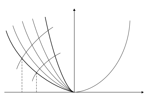
The local wave configuration around the singularity point (t,r)=(0,r0)𝑡𝑟0subscript𝑟0(t,r)=(0,r_{0}) of the GRP for (2.7) with (3.6) depends on the values of four constant vectors and consists of two nonlinear waves, each of which may be rarefaction or shock wave. Fig. 3.1 shows the schematic description of a local wave configuration: a rarefaction wave moving to the left and a shock to the right. Fig. 3.2 displays corresponding local wave configuration of the RP (3.7). In those schematic descriptions, 𝑼subscript𝑼\mbox{\boldmath\small$U$}_{*} denotes the limiting state at r=r0𝑟subscript𝑟0r=r_{0}, as t0+𝑡superscript0t\rightarrow 0^{+}, and α𝛼\alpha and β𝛽\beta are characteristic coordinate within the rarefaction wave and will be introduced in Section 3.2.1.
Refer to caption

β=βL𝛽subscript𝛽𝐿\beta=\beta_{L}β=β𝛽subscript𝛽\beta=\beta_{*}t𝑡trarefactionshockα¯¯+r0¯¯𝛼subscript𝑟0\bar{\bar{\alpha}}+r_{0}α¯+r0¯𝛼subscript𝑟0\bar{\alpha}+r_{0}α=α¯¯𝛼¯¯𝛼\alpha=\bar{\bar{\alpha}}α=α¯𝛼¯𝛼\alpha={\bar{\alpha}}𝑼L(t,r)subscript𝑼𝐿𝑡𝑟\mbox{\boldmath\small$U$}_{L}(t,r)r=r0𝑟subscript𝑟0r=r_{0}r𝑟r𝑼(t,r)subscript𝑼𝑡𝑟\mbox{\boldmath\small$U$}_{*}(t,r)𝑼R(t,r)subscript𝑼𝑅𝑡𝑟\mbox{\boldmath\small$U$}_{R}(t,r)

Figure 3.1: The schematic description of a local wave configuration for the GRP for (2.7) with (3.6) with 0t10𝑡much-less-than10\leq t\ll 1.
Refer to caption

β=βL𝛽subscript𝛽𝐿\beta=\beta_{L}β=β𝛽subscript𝛽\beta=\beta_{*}t𝑡trarefactionshockα¯¯+r0¯¯𝛼subscript𝑟0\bar{\bar{\alpha}}+r_{0}α¯+r0¯𝛼subscript𝑟0\bar{\alpha}+r_{0}α=α¯¯𝛼¯¯𝛼\alpha=\bar{\bar{\alpha}}α=α¯𝛼¯𝛼\alpha={\bar{\alpha}}𝑼Lsubscript𝑼𝐿\mbox{\boldmath\small$U$}_{L}r=r0𝑟subscript𝑟0r=r_{0}r𝑟r𝑼subscript𝑼\mbox{\boldmath\small$U$}_{*}𝑼Rsubscript𝑼𝑅\mbox{\boldmath\small$U$}_{R}

Figure 3.2: The schematic description of a local wave configuration for the associated (classical) Riemann problem (3.7).

Although there are other local wave configurations, we will restrict our discussion to the local wave configuration shown in Figs. 3.1 and 3.2. Other local wave configurations can be dealt with similarly and are considered in the code. The solutions to the GRP inside the left, intermediate and right subregions are denoted by 𝑼L(t,r),𝑼(t,r)subscript𝑼𝐿𝑡𝑟subscript𝑼𝑡𝑟\mbox{\boldmath\small$U$}_{L}(t,r),~{}\mbox{\boldmath\small$U$}_{*}(t,r), and 𝑼R(t,r)subscript𝑼𝑅𝑡𝑟\mbox{\boldmath\small$U$}_{R}(t,r), respectively. For any variable V𝑉V, which may be 𝑼𝑼U or the derivatives 𝑼tsubscript𝑼𝑡\mbox{\boldmath\small$U$}_{t} or 𝑼rsubscript𝑼𝑟\mbox{\boldmath\small$U$}_{r} etc., the symbols VLsubscript𝑉𝐿V_{L} and VRsubscript𝑉𝑅V_{R} are used to denote the limiting values of V𝑉V as t0+𝑡superscript0t\to 0^{+} in the left and right subregions adjacent to r𝑟r-axis, respectively, and Vsubscript𝑉V_{*} is used to denote the limiting values of V𝑉V as t0+𝑡superscript0t\to 0^{+} in the intermediate subregions. The main task of the direct Eulerian GRP scheme is to form a linear algebraic system

{aL(ρt)+bL(vt)=dL,aR(ρt)+bR(vt)=dR,casessubscript𝑎𝐿subscript𝜌𝑡subscript𝑏𝐿subscript𝑣𝑡subscript𝑑𝐿otherwisesubscript𝑎𝑅subscript𝜌𝑡subscript𝑏𝑅subscript𝑣𝑡subscript𝑑𝑅otherwise\begin{cases}a_{L}\left(\displaystyle{\frac{\partial\rho}{\partial t}}\right)_{*}+b_{L}\left(\displaystyle{\frac{\partial v}{\partial t}}\right)_{*}=d_{L},\\[11.38109pt] a_{R}\left(\displaystyle{\frac{\partial\rho}{\partial t}}\right)_{*}+b_{R}\left(\displaystyle{\frac{\partial v}{\partial t}}\right)_{*}=d_{R},\end{cases} (3.8)

by resolving the left wave and the right wave as shown in Figure 3.1, respectively. Solving this system gives the values of the derivatives (ρ/t)subscript𝜌𝑡(\partial\rho/\partial t)_{*} and (v/t)subscript𝑣𝑡(\partial v/\partial t)_{*}, and closes the calculation in (3.2).

3.2.1 Resolution of the rarefaction wave

This section resolves the left rarefaction wave shown in Figure 3.1 for the GRP (2.7) and (3.6), and gets the first equation in (3.8).

The relation (2.15) for the Riemann invariant ψsubscript𝜓\psi_{-} will be used to resolve the left rarefaction wave by tracking the directional derivatives DψDtsubscript𝐷subscript𝜓𝐷𝑡\frac{D_{-}\psi_{-}}{Dt} in the rarefaction fan. For this purpose, a local coordinate transformation is first introduced within the rarefaction wave, i.e. the characteristic coordinates, similar to those in [4, 12, 40]. The region of the left rarefaction wave can be described by the set :={(α(t,r),β(t,r))|β[βL,β],<α0}assignconditional-set𝛼𝑡𝑟𝛽𝑡𝑟formulae-sequence𝛽subscript𝛽𝐿subscript𝛽𝛼0{\cal R}:=\big{\{}\big{(}\alpha(t,r),\beta(t,r)\big{)}|\beta\in[\beta_{L},\beta_{*}],-\infty<\alpha\leq 0\big{\}}, where βL=λ(𝑼L)subscript𝛽𝐿subscript𝜆subscript𝑼𝐿\beta_{L}=\lambda_{-}(\mbox{\boldmath\small$U$}_{L}) and β=λ(𝑼)subscript𝛽subscript𝜆subscript𝑼\beta_{*}=\lambda_{-}(\mbox{\boldmath\small$U$}_{*}), and β=β(t,r)𝛽𝛽𝑡𝑟\beta=\beta(t,r) and α=α(t,r)𝛼𝛼𝑡𝑟\alpha=\alpha(t,r) are the integral curves of the following equations

drdt=λ,drdt=λ+,formulae-sequence𝑑𝑟𝑑𝑡subscript𝜆𝑑𝑟𝑑𝑡subscript𝜆\displaystyle{\frac{dr}{dt}}=\lambda_{-},\quad\displaystyle{\frac{dr}{dt}}=\lambda_{+}, (3.9)

respectively. Here β𝛽\beta and α𝛼\alpha have been denoted as follows: β𝛽\beta is the initial value of the slope λsubscript𝜆\lambda_{-} at the singularity point (t,r)=(0,r0)𝑡𝑟0subscript𝑟0(t,r)=(0,r_{0}), and α+r0𝛼subscript𝑟0\alpha+r_{0} for the transversal characteristic curves is the r𝑟r-coordinate of the intersection point with the leading β𝛽\beta-curve, see Figure 3.1. In this case, due to the local transformation between (t,r)𝑡𝑟(t,r) and (α,β)𝛼𝛽(\alpha,\beta), all physical quantities can be considered as functions of the local coordinates (α,β)𝛼𝛽(\alpha,\beta) and the limiting states at (t,r)=(0,0+)𝑡𝑟0limit-from0(t,r)=(0,0+) may be represented as 𝑼=𝑼(0,β)subscript𝑼𝑼0subscript𝛽\mbox{\boldmath\small$U$}_{*}=\mbox{\boldmath\small$U$}(0,\beta_{*}), etc. On the other hand, the coordinates (t,r)𝑡𝑟(t,r) inside the left rarefaction fan shown in Figure 3.1 can be expressed in terms of α𝛼\alpha and β𝛽\beta as follows

t=t(α,β),r=r(α,β).formulae-sequence𝑡𝑡𝛼𝛽𝑟𝑟𝛼𝛽t=t(\alpha,\beta),\quad r=r(\alpha,\beta).

Using the equations in (3.9) gives

rα=λtα,rβ=λ+tβ,formulae-sequence𝑟𝛼subscript𝜆𝑡𝛼𝑟𝛽subscript𝜆𝑡𝛽\displaystyle{\frac{\partial r}{\partial\alpha}}=\lambda_{-}\displaystyle{\frac{\partial t}{\partial\alpha}},\quad\displaystyle{\frac{\partial r}{\partial\beta}}=\lambda_{+}\displaystyle{\frac{\partial t}{\partial\beta}}, (3.10)

which respectively imply

α=tαDDt,β=tβD+Dt.formulae-sequence𝛼𝑡𝛼subscript𝐷𝐷𝑡𝛽𝑡𝛽subscript𝐷𝐷𝑡\displaystyle{\frac{\partial}{\partial\alpha}}=\displaystyle{\frac{\partial t}{\partial\alpha}}\displaystyle{\frac{D_{-}}{Dt}},\quad\displaystyle{\frac{\partial}{\partial\beta}}=\displaystyle{\frac{\partial t}{\partial\beta}}\displaystyle{\frac{D_{+}}{Dt}}. (3.11)

Differentiating the first equation in (3.10) with respect to β𝛽\beta and the second with respect to α𝛼\alpha may further give

2tαβ=1λ+λ(λβtαλ+αtβ).superscript2𝑡𝛼𝛽1subscript𝜆subscript𝜆subscript𝜆𝛽𝑡𝛼subscript𝜆𝛼𝑡𝛽\displaystyle{\frac{\partial^{2}t}{\partial\alpha\partial\beta}}=\displaystyle{\frac{1}{\lambda_{+}-\lambda_{-}}}\left(\displaystyle{\frac{\partial\lambda_{-}}{\partial\beta}}\displaystyle{\frac{\partial t}{\partial\alpha}}-\displaystyle{\frac{\partial\lambda_{+}}{\partial\alpha}}\displaystyle{\frac{\partial t}{\partial\beta}}\right). (3.12)

At α=0𝛼0\alpha=0, the definition of the characteristic coordinates yields

λβ(0,β)=1,tβ(0,β)=0,β[βL,β].formulae-sequencesubscript𝜆𝛽0𝛽1formulae-sequence𝑡𝛽0𝛽0for-all𝛽subscript𝛽𝐿subscript𝛽\displaystyle{\frac{\partial\lambda_{-}}{\partial\beta}}(0,\beta)=1,\quad\displaystyle{\frac{\partial t}{\partial\beta}}(0,\beta)=0,\quad\forall\beta\in[\beta_{L},\beta_{*}]. (3.13)

With the above two relations, setting α=0𝛼0\alpha=0 in (3.12) gives

2tαβ(0,β)=1λ+(0,β)λ(0,β)tα(0,β).superscript2𝑡𝛼𝛽0𝛽1subscript𝜆0𝛽subscript𝜆0𝛽𝑡𝛼0𝛽\displaystyle{\frac{\partial^{2}t}{\partial\alpha\partial\beta}}(0,\beta)=\displaystyle{\frac{1}{\lambda_{+}(0,\beta)-\lambda_{-}(0,\beta)}}\displaystyle{\frac{\partial t}{\partial\alpha}}(0,\beta). (3.14)

Our main result is given in following theorem.

Theorem 3.1

The limiting values (ρt)subscript𝜌𝑡\left(\frac{\partial\rho}{\partial t}\right)_{*} and (vt)subscript𝑣𝑡\left(\frac{\partial v}{\partial t}\right)_{*} satisfy

aL(ρt)+bL(vt)=dL,subscript𝑎𝐿subscript𝜌𝑡subscript𝑏𝐿subscript𝑣𝑡subscript𝑑𝐿a_{L}\left(\displaystyle{\frac{\partial\rho}{\partial t}}\right)_{*}+b_{L}\left(\displaystyle{\frac{\partial v}{\partial t}}\right)_{*}=d_{L}, (3.15)

where

aL=(csρ+p),bL=(11v2),formulae-sequencesubscript𝑎𝐿subscriptsubscript𝑐𝑠𝜌𝑝subscript𝑏𝐿subscript11superscript𝑣2a_{L}=\left(\frac{c_{s}}{\rho+p}\right)_{*},\quad b_{L}=\left(\frac{1}{1-v^{2}}\right)_{*}, (3.16)

and

dL=subscript𝑑𝐿absent\displaystyle d_{L}= (λ+λ+λ)(DψDt)Lexp(βLβdβ^λ+(0,β^)λ(0,β^))(λsλ+λ)subscriptsubscript𝜆subscript𝜆subscript𝜆subscriptsubscript𝐷subscript𝜓𝐷𝑡𝐿superscriptsubscriptsubscript𝛽𝐿subscript𝛽𝑑^𝛽subscript𝜆0^𝛽subscript𝜆0^𝛽subscriptsubscript𝜆subscript𝑠subscript𝜆subscript𝜆\displaystyle\left({\frac{{\lambda_{+}}}{{\lambda_{+}-\lambda_{-}}}}\right)_{*}\left(\displaystyle{\frac{D_{-}\psi_{-}}{Dt}}\right)_{L}\exp\left(-\int_{\beta_{L}}^{\beta_{*}}{\displaystyle{\frac{d\hat{\beta}}{\lambda_{+}(0,\hat{\beta})-\lambda_{-}(0,\hat{\beta})}}}\right)-\left({\frac{{\lambda_{-}s_{-}}}{{\lambda_{+}-\lambda_{-}}}}\right)_{*}
+(λ+λ+λ)βLβ(sλ+λ)(0,β^)exp(β^βdωλ+(0,ω)λ(0,ω))𝑑β^,subscriptsubscript𝜆subscript𝜆subscript𝜆superscriptsubscriptsubscript𝛽𝐿subscript𝛽subscript𝑠subscript𝜆subscript𝜆0^𝛽superscriptsubscript^𝛽subscript𝛽𝑑𝜔subscript𝜆0𝜔subscript𝜆0𝜔differential-d^𝛽\displaystyle+\left({\frac{{\lambda_{+}}}{{\lambda_{+}-\lambda_{-}}}}\right)_{*}\int_{\beta_{L}}^{\beta_{*}}\left(\frac{s_{-}}{\lambda_{+}-\lambda_{-}}\right)(0,\hat{\beta})\exp\left(-\int_{\hat{\beta}}^{\beta_{*}}\frac{d\omega}{\lambda_{+}(0,\omega)-\lambda_{-}(0,\omega)}\right)d\hat{\beta}, (3.17)

is a function of the initial data 𝐔L,𝐔Lsubscript𝐔𝐿subscriptsuperscript𝐔𝐿\mbox{\boldmath\small$U$}_{L},\mbox{\boldmath\small$U$}^{\prime}_{L}, and the limiting values 𝐔subscript𝐔\mbox{\boldmath\small$U$}_{*} or 𝐔RPsuperscript𝐔RP\mbox{\boldmath\small$U$}^{\mbox{\tiny RP}} of the (classical) Riemann problem solution 𝛚((rr0)/t,𝐔L,𝐔R)𝛚𝑟subscript𝑟0𝑡subscript𝐔𝐿subscript𝐔𝑅\mbox{\boldmath\small$\omega$}((r-r_{0})/t,\mbox{\boldmath\small$U$}_{L},\mbox{\boldmath\small$U$}_{R}).

  • Proof

    Using (2.13) and (2.15) gives

    λ+λ+λDψDtsubscript𝜆subscript𝜆subscript𝜆subscript𝐷subscript𝜓𝐷𝑡\displaystyle\frac{{\lambda_{+}}}{{\lambda_{+}-\lambda_{-}}}\frac{{D_{-}\psi_{-}}}{{Dt}} =λ+λ+λ(ψt+λψr)absentsubscript𝜆subscript𝜆subscript𝜆subscript𝜓𝑡subscript𝜆subscript𝜓𝑟\displaystyle=\frac{{\lambda_{+}}}{{\lambda_{+}-\lambda_{-}}}\left({\frac{{\partial\psi_{-}}}{{\partial t}}+\lambda_{-}\frac{{\partial\psi_{-}}}{{\partial r}}}\right)
    =ψt+λλ+λ(ψt+λ+ψr)absentsubscript𝜓𝑡subscript𝜆subscript𝜆subscript𝜆subscript𝜓𝑡subscript𝜆subscript𝜓𝑟\displaystyle=\frac{{\partial\psi_{-}}}{{\partial t}}+\frac{{\lambda_{-}}}{{\lambda_{+}-\lambda_{-}}}\left({\frac{{\partial\psi_{-}}}{{\partial t}}+\lambda_{+}\frac{{\partial\psi_{-}}}{{\partial r}}}\right)
    =11v2vt+csρ+pρt+λsλ+λ,absent11superscript𝑣2𝑣𝑡subscript𝑐𝑠𝜌𝑝𝜌𝑡subscript𝜆subscript𝑠subscript𝜆subscript𝜆\displaystyle=\frac{1}{{1-v^{2}}}\frac{{\partial v}}{{\partial t}}+\frac{{c_{s}}}{{\rho+p}}\frac{{\partial\rho}}{{\partial t}}+\frac{{\lambda_{-}s_{-}}}{{\lambda_{+}-\lambda_{-}}},

    which yields (3.15) by transposition and setting α=0,β=βformulae-sequence𝛼0𝛽subscript𝛽\alpha=0,~{}\beta=\beta_{*}, with the coefficients aL,bLsubscript𝑎𝐿subscript𝑏𝐿a_{L},b_{L} given by (3.16) and

    dL=(λ+λ+λ)DψDt(0,β)(λsλ+λ).subscript𝑑𝐿subscriptsubscript𝜆subscript𝜆subscript𝜆subscript𝐷subscript𝜓𝐷𝑡0subscript𝛽subscriptsubscript𝜆subscript𝑠subscript𝜆subscript𝜆d_{L}=\left({\frac{{\lambda_{+}}}{{\lambda_{+}-\lambda_{-}}}}\right)_{*}\frac{{D_{-}\psi_{-}}}{{Dt}}(0,\beta_{*})-\left({\frac{{\lambda_{-}s_{-}}}{{\lambda_{+}-\lambda_{-}}}}\right)_{*}. (3.18)

    Thus the following task is to complete the calculation of DψDt(0,β)subscript𝐷subscript𝜓𝐷𝑡0subscript𝛽\frac{{D_{-}\psi_{-}}}{{Dt}}(0,\beta_{*}) in (3.18). On the one hand, using the chain rule and (3.11) gives

    2ψαβ=β(tαDψDt)=2tβαDψDt+tαβ(DψDt).superscript2subscript𝜓𝛼𝛽𝛽𝑡𝛼subscript𝐷subscript𝜓𝐷𝑡superscript2𝑡𝛽𝛼subscript𝐷subscript𝜓𝐷𝑡𝑡𝛼𝛽subscript𝐷subscript𝜓𝐷𝑡\frac{{\partial^{2}\psi_{-}}}{{\partial\alpha\partial\beta}}=\frac{\partial}{{\partial\beta}}\left({\frac{{\partial t}}{{\partial\alpha}}\frac{{D_{-}\psi_{-}}}{{Dt}}}\right)=\frac{{\partial^{2}t}}{{\partial\beta\partial\alpha}}\frac{{D_{-}\psi_{-}}}{{Dt}}+\frac{{\partial t}}{{\partial\alpha}}\frac{\partial}{{\partial\beta}}\left({\frac{{D_{-}\psi_{-}}}{{Dt}}}\right). (3.19)

    On the other hand, utilizing (3.11) and (2.15), one has

    2ψαβ=α(tβD+ψDt)=α(tβs)=s2tαβ+tβsα.superscript2subscript𝜓𝛼𝛽𝛼𝑡𝛽subscript𝐷subscript𝜓𝐷𝑡𝛼𝑡𝛽subscript𝑠subscript𝑠superscript2𝑡𝛼𝛽𝑡𝛽subscript𝑠𝛼\frac{{\partial^{2}\psi_{-}}}{{\partial\alpha\partial\beta}}=\frac{\partial}{{\partial\alpha}}\left({\frac{{\partial t}}{{\partial\beta}}\frac{{D_{+}\psi_{-}}}{{Dt}}}\right)=\frac{\partial}{{\partial\alpha}}\left({\frac{{\partial t}}{{\partial\beta}}s_{-}}\right)=s_{-}\frac{{\partial^{2}t}}{{\partial\alpha\partial\beta}}+\frac{{\partial t}}{{\partial\beta}}\frac{{\partial s_{-}}}{{\partial\alpha}}. (3.20)

    Combing (3.19) and (3.20), and then setting α=0𝛼0\alpha=0 by making use of (3.13) may give

    tα(0,β)ddβ[DψDt(0,β)]=(s(0,β)DψDt(0,β))2tβα(0,β),𝑡𝛼0𝛽𝑑𝑑𝛽delimited-[]subscript𝐷subscript𝜓𝐷𝑡0𝛽subscript𝑠0𝛽subscript𝐷subscript𝜓𝐷𝑡0𝛽superscript2𝑡𝛽𝛼0𝛽\frac{{\partial t}}{{\partial\alpha}}(0,\beta)\frac{d}{{d\beta}}\left[{\frac{{D_{-}\psi_{-}}}{{Dt}}(0,\beta)}\right]=\left({s_{-}(0,\beta)-\frac{{D_{-}\psi_{-}}}{{Dt}}(0,\beta)}\right)\frac{{\partial^{2}t}}{{\partial\beta\partial\alpha}}(0,\beta),

    which further gives a ordinary differential equation at α=0𝛼0\alpha=0 for DψDt(0,β)subscript𝐷subscript𝜓𝐷𝑡0𝛽\frac{D_{-}\psi_{-}}{Dt}(0,\beta)

    ddβ[DψDt(0,β)]=1λ+λDψDt(0,β)+sλ+λ,β[βL,β],formulae-sequence𝑑𝑑𝛽delimited-[]subscript𝐷subscript𝜓𝐷𝑡0𝛽1subscript𝜆subscript𝜆subscript𝐷subscript𝜓𝐷𝑡0𝛽subscript𝑠subscript𝜆subscript𝜆𝛽subscript𝛽𝐿subscript𝛽\displaystyle{\frac{d}{{d\beta}}}\left[{\frac{{D_{-}\psi_{-}}}{{Dt}}(0,\beta)}\right]=-\displaystyle{\frac{1}{{\lambda_{+}-\lambda_{-}}}}\displaystyle{\frac{{D_{-}\psi_{-}}}{{Dt}}}(0,\beta)+\displaystyle{\frac{{s_{-}}}{{\lambda_{+}-\lambda_{-}}}},\quad\beta\in[\beta_{L},\beta_{*}], (3.21)

    by noting (3.14). Hence DψDt(0,β)subscript𝐷subscript𝜓𝐷𝑡0𝛽\frac{D_{-}\psi_{-}}{Dt}(0,\beta) can be formulated by integrating (3.21) as

    DψDt(0,β)=subscript𝐷subscript𝜓𝐷𝑡0𝛽absent\displaystyle\displaystyle{\frac{D_{-}\psi_{-}}{Dt}}(0,\beta)= (DψDt)Lexp(βLβdβ^λ+(0,β^)λ(0,β^))subscriptsubscript𝐷subscript𝜓𝐷𝑡𝐿superscriptsubscriptsubscript𝛽𝐿𝛽𝑑^𝛽subscript𝜆0^𝛽subscript𝜆0^𝛽\displaystyle\left(\displaystyle{\frac{D_{-}\psi_{-}}{Dt}}\right)_{L}\exp\left(-\int_{\beta_{L}}^{\beta}{\displaystyle{\frac{d\hat{\beta}}{\lambda_{+}(0,\hat{\beta})-\lambda_{-}(0,\hat{\beta})}}}\right)
    +βLβ(sλ+λ)(0,β^)exp(β^βdωλ+(0,ω)λ(0,ω))𝑑β^,superscriptsubscriptsubscript𝛽𝐿𝛽subscript𝑠subscript𝜆subscript𝜆0^𝛽superscriptsubscript^𝛽𝛽𝑑𝜔subscript𝜆0𝜔subscript𝜆0𝜔differential-d^𝛽\displaystyle+\int_{\beta_{L}}^{\beta}\left(\frac{s_{-}}{\lambda_{+}-\lambda_{-}}\right)(0,\hat{\beta})\exp\left(-\int_{\hat{\beta}}^{\beta}\frac{d\omega}{\lambda_{+}(0,\omega)-\lambda_{-}(0,\omega)}\right)d\hat{\beta}, (3.22)

    for all β[βL,β]𝛽subscript𝛽𝐿subscript𝛽\beta\in[\beta_{L},\beta_{*}]. Setting β=β𝛽subscript𝛽\beta=\beta_{*} in (3.22) and substituting it into (3.18) may give the expression of dLsubscript𝑑𝐿d_{L} in (3.17) and complete the proof.       

Remark 3.1

If p(ρ)=σ2ρ𝑝𝜌superscript𝜎2𝜌p(\rho)=\sigma^{2}\rho, one has λ(0,ω)=ABv(0,ω)σ1v(0,ω)σ=ωsubscript𝜆0𝜔subscript𝐴subscript𝐵𝑣0𝜔𝜎1𝑣0𝜔𝜎𝜔\lambda_{-}(0,\omega)=\sqrt{A_{*}B_{*}}\frac{v(0,\omega)-\sigma}{1-v(0,\omega)\sigma}=\omega, and

v(0,ω)=σ+ϖ1+σϖ,ϖ=ωAB,formulae-sequence𝑣0𝜔𝜎italic-ϖ1𝜎italic-ϖitalic-ϖ𝜔subscript𝐴subscript𝐵v(0,\omega)=\frac{\sigma+\varpi}{1+\sigma\varpi},\quad\varpi=\frac{\omega}{\sqrt{A_{*}B_{*}}},

For this case, the integral β^βdωλ+(0,ω)λ(0,ω)superscriptsubscript^𝛽𝛽𝑑𝜔subscript𝜆0𝜔subscript𝜆0𝜔\int_{\hat{\beta}}^{\beta}\frac{d\omega}{\lambda_{+}(0,\omega)-\lambda_{-}(0,\omega)} in (3.22) can be expressed as

β^βdωλ+(0,ω)λ(0,ω)superscriptsubscript^𝛽𝛽𝑑𝜔subscript𝜆0𝜔subscript𝜆0𝜔\displaystyle\int_{\hat{\beta}}^{\beta}\frac{d\omega}{\lambda_{+}(0,\omega)-\lambda_{-}(0,\omega)} =12σβ^/ABβ/ABσ2+1+2σϖ1ϖ2𝑑ϖabsent12𝜎superscriptsubscript^𝛽subscript𝐴subscript𝐵𝛽subscript𝐴subscript𝐵superscript𝜎212𝜎italic-ϖ1superscriptitalic-ϖ2differential-ditalic-ϖ\displaystyle=\frac{1}{2\sigma}\int_{\hat{\beta}/\sqrt{A_{*}B_{*}}}^{\beta/\sqrt{A_{*}B_{*}}}\frac{\sigma^{2}+1+2\sigma\varpi}{1-\varpi^{2}}d\varpi
=14σ[(σ1)2ln(1+ϖ)(σ+1)2ln(1ϖ)]ϖ=β^/ABϖ=β/AB.absent14𝜎superscriptsubscriptdelimited-[]superscript𝜎121italic-ϖsuperscript𝜎121italic-ϖitalic-ϖ^𝛽subscript𝐴subscript𝐵italic-ϖ𝛽subscript𝐴subscript𝐵\displaystyle=\frac{1}{4\sigma}\Big{[}(\sigma-1)^{2}\ln(1+\varpi)-(\sigma+1)^{2}\ln(1-\varpi)\Big{]}_{\varpi=\hat{\beta}/\sqrt{A_{*}B_{*}}}^{\varpi=\beta/\sqrt{A_{*}B_{*}}}.
Remark 3.2

If the right rarefaction wave associated with the eigenvalue λ+subscript𝜆\lambda_{+} appears in the GRP, then the above derivation can be used by the “reflective symmetry” transformation

ρ(r,t)=ρ~(r,t),v(r,t)=v~(r,t),p(r,t)=p~(r,t),formulae-sequence𝜌𝑟𝑡~𝜌𝑟𝑡formulae-sequence𝑣𝑟𝑡~𝑣𝑟𝑡𝑝𝑟𝑡~𝑝𝑟𝑡\rho(r,t)=\tilde{\rho}(-r,t),\ \ v(r,t)=-\tilde{v}(-r,t),\ \ p(r,t)=\tilde{p}(-r,t), (3.23)

where (ρ,v,p)Tsuperscript𝜌𝑣𝑝𝑇(\rho,v,p)^{T} and (ρ~,v~,p~)Tsuperscript~𝜌~𝑣~𝑝𝑇(\tilde{\rho},\tilde{v},\tilde{p})^{T} denote the primitive variables before and after the reflective transformation, respectively. Specially, the “reflective symmetry” transformation is first used to transfer the “real” right rarefaction wave into a “virtual” left rarefaction wave, Theorem 3.1 is then directly applied to the “virtual” left rarefaction wave, and finally using inverse transformation gives the linear equation of (ρt)subscript𝜌𝑡\big{(}\frac{\partial\rho}{\partial t}\big{)}_{*} and (vt)subscript𝑣𝑡\big{(}\frac{\partial v}{\partial t}\big{)}_{*} for the right rarefaction wave.

3.2.2 Resolution of the shock wave

This section resolves the right shock wave for the GRP (2.7) and (3.6) in Figure 3.1 and gives the second equation in (3.8) through differentiating the shock relation along the shock trajectory.

Let r=rs(t)𝑟subscript𝑟𝑠𝑡r=r_{s}(t) be the shock trajectory which is associated with the λ+subscript𝜆\lambda_{+}–characteristic field, and assume that it propagates with the speed s:=rs(t)>0assign𝑠subscriptsuperscript𝑟𝑠𝑡0s:=r^{\prime}_{s}(t)>0 to the right, see Figure 3.1. Denote the left and right states of the shock wave by 𝑼(t)𝑼𝑡\mbox{\boldmath\small$U$}(t) and 𝑼¯(t)¯𝑼𝑡\overline{\mbox{\boldmath\small$U$}}(t), respectively, i.e. 𝑼(t)=𝑼(t,rs(t)0)𝑼𝑡𝑼𝑡subscript𝑟𝑠𝑡0\mbox{\boldmath\small$U$}(t)=\mbox{\boldmath\small$U$}\big{(}t,r_{s}(t)-0\big{)} and 𝑼¯(t)=𝑼(t,rs(t)+0)¯𝑼𝑡𝑼𝑡subscript𝑟𝑠𝑡0\overline{\mbox{\boldmath\small$U$}}(t)=\mbox{\boldmath\small$U$}\big{(}t,r_{s}(t)+0\big{)}. The Rankine-Hugoniot relation across the shock wave is

[AB𝑭(𝑼)]=s[𝑼],delimited-[]𝐴𝐵𝑭𝑼𝑠delimited-[]𝑼\left[{\sqrt{AB}\mbox{\boldmath\small$F$}(\mbox{\boldmath\small$U$})}\right]=s\left[{\mbox{\boldmath\small$U$}}\right], (3.24)

or equivalently,

[𝑭(𝑼)]=(s/AB)[𝑼],delimited-[]𝑭𝑼𝑠𝐴𝐵delimited-[]𝑼\left[{\mbox{\boldmath\small$F$}(\mbox{\boldmath\small$U$})}\right]=(s/\sqrt{AB})\left[{\mbox{\boldmath\small$U$}}\right], (3.25)

where []delimited-[]\left[{\cdot}\right] denotes the jump across the shock wave, and the continuity of AB𝐴𝐵\sqrt{AB} has been used. Utilizing this relation gives

vv¯1vv¯=Φ(ρ,ρ¯),𝑣¯𝑣1𝑣¯𝑣Φ𝜌¯𝜌\displaystyle{\frac{v-\bar{v}}{1-v\bar{v}}}=\Phi(\rho,\bar{\rho}), (3.26)

where

Φ(ρ,ρ¯):=(pp¯)(ρρ¯)(ρ+p¯)(ρ¯+p),assignΦ𝜌¯𝜌𝑝¯𝑝𝜌¯𝜌𝜌¯𝑝¯𝜌𝑝\Phi(\rho,\bar{\rho}):=\sqrt{\displaystyle{\frac{(p-\bar{p})(\rho-\bar{\rho})}{(\rho+\bar{p})(\bar{\rho}+p)}}}, (3.27)

see [11] for the detailed derivation. Thus along the shock trajectory, one always has

DsDt(vv¯1vv¯)=DsDtΦ(ρ,ρ¯),subscript𝐷𝑠𝐷𝑡𝑣¯𝑣1𝑣¯𝑣subscript𝐷𝑠𝐷𝑡Φ𝜌¯𝜌\displaystyle{\frac{D_{s}}{Dt}}\Big{(}\displaystyle{\frac{v-\bar{v}}{1-v\bar{v}}}\Big{)}=\displaystyle{\frac{D_{s}}{Dt}}\Phi(\rho,\bar{\rho}), (3.28)

where DsDt:=t+sxassignsubscript𝐷𝑠𝐷𝑡𝑡𝑠𝑥\frac{D_{s}}{Dt}:=\frac{\partial}{\partial t}+s\frac{\partial}{\partial x} denotes the directional derivative along the shock trajectory.

The main result in this subsection is given as follows.

Theorem 3.2

The limiting values of (ρt)subscript𝜌𝑡\left(\frac{\partial\rho}{\partial t}\right)_{*} and (vt)subscript𝑣𝑡\left(\frac{\partial v}{\partial t}\right)_{*} satisfy

aR(ρt)+bR(vt)=dR,subscript𝑎𝑅subscript𝜌𝑡subscript𝑏𝑅subscript𝑣𝑡subscript𝑑𝑅a_{R}\left(\displaystyle{\frac{\partial\rho}{\partial t}}\right)_{*}+b_{R}\left(\displaystyle{\frac{\partial v}{\partial t}}\right)_{*}=d_{R}, (3.29)

where the expressions of the coefficients aR,bRsubscript𝑎𝑅subscript𝑏𝑅a_{R},b_{R}, and dRsubscript𝑑𝑅d_{R} will be given in the proof.

  • Proof

    Utilizing (2.14), one has

    (v2cs2sv(1cs2)ABs(ρ+p)ABs(1v2)2cs2AB(ρ+p)v2cs2sv(1cs2)AB)𝑽tsuperscript𝑣2superscriptsubscript𝑐𝑠2𝑠𝑣1superscriptsubscript𝑐𝑠2𝐴𝐵𝑠𝜌𝑝𝐴𝐵missing-subexpressionmissing-subexpressionmissing-subexpressionmissing-subexpressionmissing-subexpressionmissing-subexpressionmissing-subexpressionmissing-subexpressionmissing-subexpressionmissing-subexpressionmissing-subexpressionmissing-subexpressionmissing-subexpressionmissing-subexpressionmissing-subexpressionmissing-subexpressionmissing-subexpressionmissing-subexpression𝑠superscript1superscript𝑣22superscriptsubscript𝑐𝑠2𝐴𝐵𝜌𝑝superscript𝑣2superscriptsubscript𝑐𝑠2𝑠𝑣1superscriptsubscript𝑐𝑠2𝐴𝐵missing-subexpressionmissing-subexpressionmissing-subexpressionmissing-subexpressionmissing-subexpressionmissing-subexpressionmissing-subexpressionmissing-subexpressionmissing-subexpressionmissing-subexpressionmissing-subexpressionmissing-subexpressionmissing-subexpressionmissing-subexpressionmissing-subexpressionmissing-subexpressionmissing-subexpressionmissing-subexpression𝑽𝑡\displaystyle\left({\begin{array}[]{*{20}c}{v^{2}-c_{s}^{2}-\frac{{sv(1-c_{s}^{2})}}{{\sqrt{AB}}}}&{\frac{{s(\rho+p)}}{{\sqrt{AB}}}}\\ {\frac{{s(1-v^{2})^{2}c_{s}^{2}}}{{\sqrt{AB}(\rho+p)}}}&{v^{2}-c_{s}^{2}-\frac{{sv(1-c_{s}^{2})}}{{\sqrt{AB}}}}\end{array}}\right)\frac{{\partial\mbox{\boldmath\small$V$}}}{{\partial t}} (3.32)
    =(v2cs2)𝑽tsAB(v(1cs2)(ρ+p)(1v2)2cs2(ρ+p)v(1cs2))𝑽tabsentsuperscript𝑣2superscriptsubscript𝑐𝑠2𝑽𝑡𝑠𝐴𝐵𝑣1superscriptsubscript𝑐𝑠2𝜌𝑝missing-subexpressionmissing-subexpressionmissing-subexpressionmissing-subexpressionmissing-subexpressionmissing-subexpressionmissing-subexpressionmissing-subexpressionmissing-subexpressionmissing-subexpressionmissing-subexpressionmissing-subexpressionmissing-subexpressionmissing-subexpressionmissing-subexpressionmissing-subexpressionmissing-subexpressionmissing-subexpressionsuperscript1superscript𝑣22superscriptsubscript𝑐𝑠2𝜌𝑝𝑣1superscriptsubscript𝑐𝑠2missing-subexpressionmissing-subexpressionmissing-subexpressionmissing-subexpressionmissing-subexpressionmissing-subexpressionmissing-subexpressionmissing-subexpressionmissing-subexpressionmissing-subexpressionmissing-subexpressionmissing-subexpressionmissing-subexpressionmissing-subexpressionmissing-subexpressionmissing-subexpressionmissing-subexpressionmissing-subexpression𝑽𝑡\displaystyle=\left({v^{2}-c_{s}^{2}}\right)\frac{{\partial\mbox{\boldmath\small$V$}}}{{\partial t}}-\frac{s}{{\sqrt{AB}}}\left({\begin{array}[]{*{20}c}{v(1-c_{s}^{2})}&{-(\rho+p)}\\ {-\frac{{(1-v^{2})^{2}c_{s}^{2}}}{{(\rho+p)}}}&{v(1-c_{s}^{2})}\end{array}}\right)\frac{{\partial\mbox{\boldmath\small$V$}}}{{\partial t}} (3.35)
    =(v2cs2)𝑽tsAB(v(1cs2)(ρ+p)(1v2)2cs2(ρ+p)v(1cs2))(𝑯𝑱𝑽r)absentsuperscript𝑣2superscriptsubscript𝑐𝑠2𝑽𝑡𝑠𝐴𝐵𝑣1superscriptsubscript𝑐𝑠2𝜌𝑝missing-subexpressionmissing-subexpressionmissing-subexpressionmissing-subexpressionmissing-subexpressionmissing-subexpressionmissing-subexpressionmissing-subexpressionmissing-subexpressionmissing-subexpressionmissing-subexpressionmissing-subexpressionmissing-subexpressionmissing-subexpressionmissing-subexpressionmissing-subexpressionmissing-subexpressionmissing-subexpressionsuperscript1superscript𝑣22superscriptsubscript𝑐𝑠2𝜌𝑝𝑣1superscriptsubscript𝑐𝑠2missing-subexpressionmissing-subexpressionmissing-subexpressionmissing-subexpressionmissing-subexpressionmissing-subexpressionmissing-subexpressionmissing-subexpressionmissing-subexpressionmissing-subexpressionmissing-subexpressionmissing-subexpressionmissing-subexpressionmissing-subexpressionmissing-subexpressionmissing-subexpressionmissing-subexpressionmissing-subexpression𝑯𝑱𝑽𝑟\displaystyle=\left({v^{2}-c_{s}^{2}}\right)\frac{{\partial\mbox{\boldmath\small$V$}}}{{\partial t}}-\frac{s}{{\sqrt{AB}}}\left({\begin{array}[]{*{20}c}{v(1-c_{s}^{2})}&{-(\rho+p)}\\ {-\frac{{(1-v^{2})^{2}c_{s}^{2}}}{{(\rho+p)}}}&{v(1-c_{s}^{2})}\end{array}}\right)\left({\mbox{\boldmath\small$H$}-\mbox{\boldmath\small$J$}\frac{{\partial\mbox{\boldmath\small$V$}}}{{\partial r}}}\right) (3.38)
    =(v2cs2)(𝑽t+s𝑽r)sAB(v(1cs2)H1(ρ+p)H2(1v2)2cs2(ρ+p)H1+v(1cs2)H2)absentsuperscript𝑣2superscriptsubscript𝑐𝑠2𝑽𝑡𝑠𝑽𝑟𝑠𝐴𝐵𝑣1superscriptsubscript𝑐𝑠2subscript𝐻1𝜌𝑝subscript𝐻2superscript1superscript𝑣22superscriptsubscript𝑐𝑠2𝜌𝑝subscript𝐻1𝑣1superscriptsubscript𝑐𝑠2subscript𝐻2\displaystyle=\left({v^{2}-c_{s}^{2}}\right)\left({\frac{{\partial\mbox{\boldmath\small$V$}}}{{\partial t}}+s\frac{{\partial\mbox{\boldmath\small$V$}}}{{\partial r}}}\right)-\frac{s}{{\sqrt{AB}}}\left(\begin{array}[]{l}v(1-c_{s}^{2})H_{1}-(\rho+p)H_{2}\\ -\frac{{(1-v^{2})^{2}c_{s}^{2}}}{{(\rho+p)}}H_{1}+v(1-c_{s}^{2})H_{2}\end{array}\right) (3.41)
    =(v2cs2)Ds𝑽Dt+sr((ρ+p)(2v2(1A)(1v2)2Aκr2(p+ρv2)2A)v(v21)(2cs2(1A)(1cs2)2Aκr2(p+ρcs2)2A))absentsuperscript𝑣2superscriptsubscript𝑐𝑠2subscript𝐷𝑠𝑽𝐷𝑡𝑠𝑟𝜌𝑝2superscript𝑣21𝐴1superscript𝑣22𝐴𝜅superscript𝑟2𝑝𝜌superscript𝑣22𝐴𝑣superscript𝑣212superscriptsubscript𝑐𝑠21𝐴1superscriptsubscript𝑐𝑠22𝐴𝜅superscript𝑟2𝑝𝜌superscriptsubscript𝑐𝑠22𝐴\displaystyle=\left({v^{2}-c_{s}^{2}}\right)\frac{{D_{s}\mbox{\boldmath\small$V$}}}{{Dt}}+\frac{s}{r}\left(\begin{array}[]{l}(\rho+p)\left({2v^{2}-\frac{{(1-A)(1-v^{2})}}{{2A}}-\frac{{\kappa r^{2}(p+\rho v^{2})}}{{2A}}}\right)\\ v(v^{2}-1)\left({2c_{s}^{2}-\frac{{(1-A)(1-c_{s}^{2})}}{{2A}}-\frac{{\kappa r^{2}(p+\rho c_{s}^{2})}}{{2A}}}\right)\\ \end{array}\right) (3.44)
    =:(v2cs2)Ds𝑽Dt+(Π1,Π2)T,\displaystyle=:\left({v^{2}-c_{s}^{2}}\right)\frac{{D_{s}\mbox{\boldmath\small$V$}}}{{Dt}}+(\Pi_{1},\Pi_{2})^{\rm T}, (3.45)

    with which a relation between t𝑡\frac{\partial}{\partial t} and DsDtsubscript𝐷𝑠𝐷𝑡\frac{D_{s}}{Dt} is established. The following will expand (3.28) by the chain rule and use the relation (3.45) to transfer the derivatives along the shock trajectory to the time derivatives for the left state of the shock wave. The left and right hand sides of (3.28) will be treated separately.

    The left hand side of (3.28) can be rewritten as

    DsDt(vv¯1vv¯)=1v¯2(1vv¯)2DsvDt1v2(1vv¯)2Dsv¯Dt.subscript𝐷𝑠𝐷𝑡𝑣¯𝑣1𝑣¯𝑣1superscript¯𝑣2superscript1𝑣¯𝑣2subscript𝐷𝑠𝑣𝐷𝑡1superscript𝑣2superscript1𝑣¯𝑣2subscript𝐷𝑠¯𝑣𝐷𝑡\displaystyle\displaystyle{\frac{D_{s}}{Dt}}\Big{(}\displaystyle{\frac{v-\bar{v}}{1-v\bar{v}}}\Big{)}=\displaystyle{\frac{1-\bar{v}^{2}}{(1-v\bar{v})^{2}}}\displaystyle{\frac{D_{s}v}{Dt}}-\displaystyle{\frac{1-v^{2}}{(1-v\bar{v})^{2}}}\displaystyle{\frac{D_{s}\bar{v}}{Dt}}.

    If considering p𝑝p as a function of ρ𝜌\rho, i.e. p=p(ρ)𝑝𝑝𝜌p=p(\rho), then the right hand side of (3.28) may be expanded as

    DsDtΦ(ρ,ρ¯)=Φρ(ρ,ρ¯)DsρDt+Φρ¯(ρ,ρ¯)Dsρ¯Dt,subscript𝐷𝑠𝐷𝑡Φ𝜌¯𝜌subscriptΦ𝜌𝜌¯𝜌subscript𝐷𝑠𝜌𝐷𝑡subscriptΦ¯𝜌𝜌¯𝜌subscript𝐷𝑠¯𝜌𝐷𝑡\frac{{D_{s}}}{{Dt}}\Phi(\rho,\bar{\rho})=\Phi_{\rho}(\rho,\bar{\rho})\frac{{D_{s}\rho}}{{Dt}}+\Phi_{\bar{\rho}}(\rho,\bar{\rho})\frac{{D_{s}\bar{\rho}}}{{Dt}},

    where

    Φρ(ρ,ρ¯)subscriptΦ𝜌𝜌¯𝜌\displaystyle\Phi_{\rho}(\rho,\bar{\rho}) =(ρ¯+p¯)(cs2Δρ,ρ¯1(ρ+p¯)+Δρ,ρ¯(ρ¯+p))2((ρ+p¯)(ρ¯+p))32,absent¯𝜌¯𝑝superscriptsubscript𝑐𝑠2superscriptsubscriptΔ𝜌¯𝜌1𝜌¯𝑝subscriptΔ𝜌¯𝜌¯𝜌𝑝2superscript𝜌¯𝑝¯𝜌𝑝32\displaystyle=\frac{{(\bar{\rho}+\bar{p})\left({c_{s}^{2}\Delta_{\rho,\bar{\rho}}^{-1}(\rho+\bar{p})+\Delta_{\rho,\bar{\rho}}(\bar{\rho}+p)}\right)}}{{2\left({(\rho+\bar{p})(\bar{\rho}+p)}\right)^{\frac{3}{2}}}},
    Φρ¯(ρ,ρ¯)subscriptΦ¯𝜌𝜌¯𝜌\displaystyle\Phi_{\bar{\rho}}(\rho,\bar{\rho}) =(ρ+p)(c¯s2Δρ,ρ¯1(ρ¯+p)+Δρ,ρ¯(ρ+p¯))2((ρ+p¯)(ρ¯+p))32,absent𝜌𝑝superscriptsubscript¯𝑐𝑠2superscriptsubscriptΔ𝜌¯𝜌1¯𝜌𝑝subscriptΔ𝜌¯𝜌𝜌¯𝑝2superscript𝜌¯𝑝¯𝜌𝑝32\displaystyle=-\frac{{(\rho+p)\left({\bar{c}_{s}^{2}\Delta_{\rho,\bar{\rho}}^{-1}(\bar{\rho}+p)+\Delta_{\rho,\bar{\rho}}(\rho+\bar{p})}\right)}}{{2\left({(\rho+\bar{p})(\bar{\rho}+p)}\right)^{\frac{3}{2}}}},

    with Δρ,ρ¯:=(pp¯)/(ρρ¯)assignsubscriptΔ𝜌¯𝜌𝑝¯𝑝𝜌¯𝜌\Delta_{\rho,\bar{\rho}}:=\sqrt{(p-\bar{p})/(\rho-\bar{\rho})}. Therefore, (3.28) is equivalent to

    Φρ(ρ,ρ¯)DsρDt+v¯21(1vv¯)2DsvDt=v21(1vv¯)2Dsv¯DtΦρ¯(ρ,ρ¯)Dsρ¯Dt.subscriptΦ𝜌𝜌¯𝜌subscript𝐷𝑠𝜌𝐷𝑡superscript¯𝑣21superscript1𝑣¯𝑣2subscript𝐷𝑠𝑣𝐷𝑡superscript𝑣21superscript1𝑣¯𝑣2subscript𝐷𝑠¯𝑣𝐷𝑡subscriptΦ¯𝜌𝜌¯𝜌subscript𝐷𝑠¯𝜌𝐷𝑡\Phi_{\rho}(\rho,\bar{\rho})\frac{{D_{s}\rho}}{{Dt}}+\displaystyle{\frac{\bar{v}^{2}-1}{(1-v\bar{v})^{2}}}\displaystyle{\frac{D_{s}v}{Dt}}=\displaystyle{\frac{v^{2}-1}{(1-v\bar{v})^{2}}}\displaystyle{\frac{D_{s}\bar{v}}{Dt}}-\Phi_{\bar{\rho}}(\rho,\bar{\rho})\frac{{D_{s}\bar{\rho}}}{{Dt}}. (3.46)

    Multiplying both sides of (3.45) with the row vector (Φρ(ρ,ρ¯),v¯21(1vv¯)2),subscriptΦ𝜌𝜌¯𝜌superscript¯𝑣21superscript1𝑣¯𝑣2\left(\Phi_{\rho}(\rho,\bar{\rho}),\frac{\bar{v}^{2}-1}{(1-v\bar{v})^{2}}\right), and then substituting (3.46) into it, we have

    (Φρ(ρ,ρ¯),v¯21(1vv¯)2)(v2cs2sv(1cs2)ABs(ρ+p)ABs(1v2)2cs2AB(ρ+p)v2cs2sv(1cs2)AB)𝑽tsubscriptΦ𝜌𝜌¯𝜌superscript¯𝑣21superscript1𝑣¯𝑣2superscript𝑣2superscriptsubscript𝑐𝑠2𝑠𝑣1superscriptsubscript𝑐𝑠2𝐴𝐵𝑠𝜌𝑝𝐴𝐵missing-subexpressionmissing-subexpressionmissing-subexpressionmissing-subexpressionmissing-subexpressionmissing-subexpressionmissing-subexpressionmissing-subexpressionmissing-subexpressionmissing-subexpressionmissing-subexpressionmissing-subexpressionmissing-subexpressionmissing-subexpressionmissing-subexpressionmissing-subexpressionmissing-subexpressionmissing-subexpression𝑠superscript1superscript𝑣22superscriptsubscript𝑐𝑠2𝐴𝐵𝜌𝑝superscript𝑣2superscriptsubscript𝑐𝑠2𝑠𝑣1superscriptsubscript𝑐𝑠2𝐴𝐵missing-subexpressionmissing-subexpressionmissing-subexpressionmissing-subexpressionmissing-subexpressionmissing-subexpressionmissing-subexpressionmissing-subexpressionmissing-subexpressionmissing-subexpressionmissing-subexpressionmissing-subexpressionmissing-subexpressionmissing-subexpressionmissing-subexpressionmissing-subexpressionmissing-subexpressionmissing-subexpression𝑽𝑡\displaystyle\bigg{(}\Phi_{\rho}(\rho,\bar{\rho}),\displaystyle{\frac{\bar{v}^{2}-1}{(1-v\bar{v})^{2}}}\bigg{)}\left({\begin{array}[]{*{20}c}{v^{2}-c_{s}^{2}-\frac{{sv(1-c_{s}^{2})}}{{\sqrt{AB}}}}&{\frac{{s(\rho+p)}}{{\sqrt{AB}}}}\\ {\frac{{s(1-v^{2})^{2}c_{s}^{2}}}{{\sqrt{AB}(\rho+p)}}}&{v^{2}-c_{s}^{2}-\frac{{sv(1-c_{s}^{2})}}{{\sqrt{AB}}}}\end{array}}\right)\frac{{\partial\mbox{\boldmath\small$V$}}}{{\partial t}} (3.49)
    =(v2cs2)(Φρ(ρ,ρ¯)DsρDt+v¯21(1vv¯)2DsvDt)+Φρ(ρ,ρ¯)Π1+v¯21(1vv¯)2Π2absentsuperscript𝑣2superscriptsubscript𝑐𝑠2subscriptΦ𝜌𝜌¯𝜌subscript𝐷𝑠𝜌𝐷𝑡superscript¯𝑣21superscript1𝑣¯𝑣2subscript𝐷𝑠𝑣𝐷𝑡subscriptΦ𝜌𝜌¯𝜌subscriptΠ1superscript¯𝑣21superscript1𝑣¯𝑣2subscriptΠ2\displaystyle=(v^{2}-c_{s}^{2})\bigg{(}\Phi_{\rho}(\rho,\bar{\rho})\frac{{D_{s}\rho}}{{Dt}}+\displaystyle{\frac{\bar{v}^{2}-1}{(1-v\bar{v})^{2}}}\displaystyle{\frac{D_{s}v}{Dt}}\bigg{)}+\Phi_{\rho}(\rho,\bar{\rho})\Pi_{1}+\displaystyle{\frac{\bar{v}^{2}-1}{(1-v\bar{v})^{2}}}\Pi_{2}
    =(v2cs2)(v21(1vv¯)2Dsv¯DtΦρ¯(ρ,ρ¯)Dsρ¯Dt)+Φρ(ρ,ρ¯)Π1+v¯21(1vv¯)2Π2.absentsuperscript𝑣2superscriptsubscript𝑐𝑠2superscript𝑣21superscript1𝑣¯𝑣2subscript𝐷𝑠¯𝑣𝐷𝑡subscriptΦ¯𝜌𝜌¯𝜌subscript𝐷𝑠¯𝜌𝐷𝑡subscriptΦ𝜌𝜌¯𝜌subscriptΠ1superscript¯𝑣21superscript1𝑣¯𝑣2subscriptΠ2\displaystyle=(v^{2}-c_{s}^{2})\bigg{(}\displaystyle{\frac{v^{2}-1}{(1-v\bar{v})^{2}}}\displaystyle{\frac{D_{s}\bar{v}}{Dt}}-\Phi_{\bar{\rho}}(\rho,\bar{\rho})\frac{{D_{s}\bar{\rho}}}{{Dt}}\bigg{)}+\Phi_{\rho}(\rho,\bar{\rho})\Pi_{1}+\displaystyle{\frac{\bar{v}^{2}-1}{(1-v\bar{v})^{2}}}\Pi_{2}. (3.50)

    Setting t0+𝑡superscript0t\to 0^{+} in (3.50) gives (3.29) with

    aRsubscript𝑎𝑅\displaystyle a_{R} =Φρ(ρ,ρR)(v2cs2sv(1cs2)AB)+vR21(1vvR)2(s(1v2)2cs2AB(ρ+p)),absentsubscriptΦ𝜌subscript𝜌subscript𝜌𝑅subscriptsuperscript𝑣2superscriptsubscript𝑐𝑠2𝑠𝑣1superscriptsubscript𝑐𝑠2𝐴𝐵subscriptsuperscript𝑣2𝑅1superscript1subscript𝑣subscript𝑣𝑅2subscript𝑠superscript1superscript𝑣22superscriptsubscript𝑐𝑠2𝐴𝐵𝜌𝑝\displaystyle=\Phi_{\rho}(\rho_{*},\rho_{R})\left({v^{2}-c_{s}^{2}-\frac{{sv(1-c_{s}^{2})}}{{\sqrt{AB}}}}\right)_{*}+\displaystyle{\frac{v^{2}_{R}-1}{(1-v_{*}v_{R})^{2}}}\left({\frac{{s(1-v^{2})^{2}c_{s}^{2}}}{{\sqrt{AB}(\rho+p)}}}\right)_{*}, (3.51)
    bRsubscript𝑏𝑅\displaystyle b_{R} =Φρ(ρ,ρR)s(ρ+p)AB+vR21(1vvR)2(v2cs2sv(1cs2)AB),absentsubscriptΦ𝜌subscript𝜌subscript𝜌𝑅subscript𝑠subscript𝜌subscript𝑝subscript𝐴subscript𝐵subscriptsuperscript𝑣2𝑅1superscript1subscript𝑣subscript𝑣𝑅2subscriptsuperscript𝑣2superscriptsubscript𝑐𝑠2𝑠𝑣1superscriptsubscript𝑐𝑠2𝐴𝐵\displaystyle=\Phi_{\rho}(\rho_{*},\rho_{R}){\frac{{s_{*}(\rho_{*}+p_{*})}}{{\sqrt{A_{*}B_{*}}}}}+\displaystyle{\frac{v^{2}_{R}-1}{(1-v_{*}v_{R})^{2}}}\left({v^{2}-c_{s}^{2}-\frac{{sv(1-c_{s}^{2})}}{{\sqrt{AB}}}}\right)_{*}, (3.52)

    and

    dR=subscript𝑑𝑅absent\displaystyle d_{R}= Φρ(ρ,ρR)(Π1)+vR21(1vvR)2(Π2)subscriptΦ𝜌subscript𝜌subscript𝜌𝑅subscriptsubscriptΠ1subscriptsuperscript𝑣2𝑅1superscript1subscript𝑣subscript𝑣𝑅2subscriptsubscriptΠ2\displaystyle\Phi_{\rho}(\rho_{*},\rho_{R})(\Pi_{1})_{*}+\displaystyle{\frac{v^{2}_{R}-1}{(1-v_{*}v_{R})^{2}}}(\Pi_{2})_{*}
    +(v2cs2)[v21(1vvR)2(DsvDt)RΦρ¯(ρ,ρR)(DsρDt)R],\displaystyle+(v^{2}-c_{s}^{2})_{*}\left[\displaystyle{\frac{v^{2}_{*}-1}{(1-v_{*}v_{R})^{2}}}\left(\displaystyle{\frac{D_{s}v}{Dt}}\bigg{)}_{R}-\Phi_{\bar{\rho}}(\rho_{*},\rho_{R})\right(\frac{{D_{s}\rho}}{{Dt}}\bigg{)}_{R}\right],

    where ssubscript𝑠s_{*} denotes the initial value of the slope of the shock trajectory. The proof is completed.       

Remark 3.3

Similarly, if the left shock wave associated with the eigenvalue λsubscript𝜆\lambda_{-} appears in the GRP, then Theorem 3.2 may be applied to the “virtual” right shock wave obtained by using the “reflective symmetry” transformation (3.23), and corresponding inverse transformation is finally used to give the linear equation of the limiting values (ρt)subscript𝜌𝑡\big{(}\frac{\partial\rho}{\partial t}\big{)}_{*} and (vt)subscript𝑣𝑡\big{(}\frac{\partial v}{\partial t}\big{)}_{*}.

3.2.3 Time derivatives of solutions at singularity point

This subsection is devoted to derive the time derivatives (𝑼/t)subscript𝑼𝑡\left({\partial\mbox{\boldmath\small$U$}}/{\partial t}\right)_{*} and complete the calculation in (3.2).

I. Nonsonic case

The discussion in this part is only restricted to the case of the local wave configuration in Fig. 3.1, in which λ(𝑼)<0subscript𝜆subscript𝑼0\lambda_{-}(\mbox{\boldmath\small$U$}_{*})<0, that is to say, the t𝑡t-axis locates at the right hand side of the rarefaction wave. Other (possible) nonsonic local wave configurations can be similarly discussed and should be implemented in the code, while the case of the transonic rarefaction wave will be discussed later.

Theorem 3.3

Under the assumption that λ(𝐔)<0subscript𝜆subscript𝐔0\lambda_{-}(\mbox{\boldmath\small$U$}_{*})<0 and s>0subscript𝑠0s_{*}>0, the 2×2222\times 2 linear system formed by (3.15) in Theorem 3.1 and (3.29) in Theorem 3.2 has unique solution.

  • Proof

    It only needs to check

    det(aLbLaRbR)=aLbRaRbL0,subscript𝑎𝐿subscript𝑏𝐿missing-subexpressionmissing-subexpressionmissing-subexpressionmissing-subexpressionmissing-subexpressionmissing-subexpressionmissing-subexpressionmissing-subexpressionmissing-subexpressionmissing-subexpressionmissing-subexpressionmissing-subexpressionmissing-subexpressionmissing-subexpressionmissing-subexpressionmissing-subexpressionmissing-subexpressionmissing-subexpressionsubscript𝑎𝑅subscript𝑏𝑅missing-subexpressionmissing-subexpressionmissing-subexpressionmissing-subexpressionmissing-subexpressionmissing-subexpressionmissing-subexpressionmissing-subexpressionmissing-subexpressionmissing-subexpressionmissing-subexpressionmissing-subexpressionmissing-subexpressionmissing-subexpressionmissing-subexpressionmissing-subexpressionmissing-subexpressionmissing-subexpressionsubscript𝑎𝐿subscript𝑏𝑅subscript𝑎𝑅subscript𝑏𝐿0\det\left({\begin{array}[]{*{20}c}{a_{L}}&{b_{L}}\\ {a_{R}}&{b_{R}}\end{array}}\right)=a_{L}b_{R}-a_{R}b_{L}\neq 0,

    which is sufficiently ensured if aLbLaRbR<0subscript𝑎𝐿subscript𝑏𝐿subscript𝑎𝑅subscript𝑏𝑅0a_{L}b_{L}a_{R}b_{R}<0. It is obvious that aLbL>0subscript𝑎𝐿subscript𝑏𝐿0a_{L}b_{L}>0 due to (3.16). Thus if aRbR<0subscript𝑎𝑅subscript𝑏𝑅0a_{R}b_{R}<0, then the proof may be completed. Before that, we first prove the following inequality

    (v2cs2sv(1cs2)AB)<0.subscriptsuperscript𝑣2superscriptsubscript𝑐𝑠2𝑠𝑣1superscriptsubscript𝑐𝑠2𝐴𝐵0\left({v^{2}-c_{s}^{2}-\frac{{sv(1-c_{s}^{2})}}{{\sqrt{AB}}}}\right)_{*}<0. (3.53)

    The Lax entropy inequality for the right shock wave

    (ABv+cs1+vcs)>s>(ABv+cs1+vcs)R,subscript𝐴𝐵𝑣subscript𝑐𝑠1𝑣subscript𝑐𝑠subscript𝑠subscript𝐴𝐵𝑣subscript𝑐𝑠1𝑣subscript𝑐𝑠𝑅\left(\sqrt{AB}\displaystyle{\frac{v+c_{s}}{1+vc_{s}}}\right)_{*}>s_{*}>\left(\sqrt{AB}\displaystyle{\frac{v+c_{s}}{1+vc_{s}}}\right)_{R}, (3.54)

    implies (v+cs)>0subscript𝑣subscript𝑐𝑠0(v+c_{s})_{*}>0 due to s>0subscript𝑠0s_{*}>0. If v0subscript𝑣0v_{*}\leq 0, with the left inequality in (3.54), one has

    (sv(1cs2)AB)((v+cs)v(1cs2)1+vcs)=(v2cs2+cs(v+cs)(1v2)1+vcs)>(v2cs2),subscript𝑠𝑣1superscriptsubscript𝑐𝑠2𝐴𝐵subscript𝑣subscript𝑐𝑠𝑣1superscriptsubscript𝑐𝑠21𝑣subscript𝑐𝑠subscriptsuperscript𝑣2superscriptsubscript𝑐𝑠2subscript𝑐𝑠𝑣subscript𝑐𝑠1superscript𝑣21𝑣subscript𝑐𝑠subscriptsuperscript𝑣2superscriptsubscript𝑐𝑠2\displaystyle\left({\frac{{sv(1-c_{s}^{2})}}{{\sqrt{AB}}}}\right)_{*}\geq\left({\frac{{(v+c_{s})v(1-c_{s}^{2})}}{{1+vc_{s}}}}\right)_{*}=\left(v^{2}-c_{s}^{2}+{\frac{{c_{s}(v+c_{s})(1-v^{2})}}{{1+vc_{s}}}}\right)_{*}>(v^{2}-c_{s}^{2})_{*},

    where (v+cs)>0subscript𝑣subscript𝑐𝑠0(v+c_{s})_{*}>0 has been used in the last inequality. If v>0subscript𝑣0v_{*}>0, then one has

    (v2cs2sv(1cs2)AB)<(v2cs2)=λ(𝑼)(v+cs)(1vcsAB)<0,subscriptsuperscript𝑣2superscriptsubscript𝑐𝑠2𝑠𝑣1superscriptsubscript𝑐𝑠2𝐴𝐵subscriptsuperscript𝑣2superscriptsubscript𝑐𝑠2subscript𝜆subscript𝑼subscript𝑣subscript𝑐𝑠subscript1𝑣subscript𝑐𝑠𝐴𝐵0\left({v^{2}-c_{s}^{2}-\frac{{sv(1-c_{s}^{2})}}{{\sqrt{AB}}}}\right)_{*}<(v^{2}-c_{s}^{2})_{*}=\lambda_{-}(\mbox{\boldmath\small$U$}_{*})\left({v+c_{s}}\right)_{*}\left({\frac{{1-vc_{s}}}{{\sqrt{AB}}}}\right)_{*}<0,

    where λ(𝑼)<0subscript𝜆subscript𝑼0\lambda_{-}(\mbox{\boldmath\small$U$}_{*})<0 and (v+cs)>0subscript𝑣subscript𝑐𝑠0(v+c_{s})_{*}>0 have been used in the last inequality. Hence the inequality (3.53) holds for any vsubscript𝑣v_{*}. The expressions of aRsubscript𝑎𝑅a_{R} in (3.51) and bRsubscript𝑏𝑅b_{R} in (3.52), and vR<1subscript𝑣𝑅1v_{R}<1 and Φρ(ρ,ρR)>0subscriptΦ𝜌subscript𝜌subscript𝜌𝑅0\Phi_{\rho}(\rho_{*},\rho_{R})>0 imply that aR<0subscript𝑎𝑅0a_{R}<0 and bR>0subscript𝑏𝑅0b_{R}>0. Therefore aLbLaRbR<0subscript𝑎𝐿subscript𝑏𝐿subscript𝑎𝑅subscript𝑏𝑅0a_{L}b_{L}a_{R}b_{R}<0 and the proof is completed.       

II. Sonic case

Next, discuss the sonic case of that the t𝑡t-axis is within the left rarefaction region in Fig. 3.1. In this case, the t𝑡t-axis is actually tangential to the λsubscript𝜆\lambda_{-}-characteristic curve with zero initial slope, i.e. λ(0,β)=0subscript𝜆0subscript𝛽0\lambda_{-}(0,\beta_{*})=0 or β=0subscript𝛽0\beta_{*}=0. Then one has

(𝑼t)=D𝑼Dt(0,β),subscript𝑼𝑡subscript𝐷𝑼𝐷𝑡0subscript𝛽\left(\displaystyle{\frac{\partial\mbox{\boldmath\small$U$}}{\partial t}}\right)_{*}=\displaystyle{\frac{D_{-}\mbox{\boldmath\small$U$}}{Dt}}(0,\beta_{*}),

for β=0subscript𝛽0\beta_{*}=0.

Theorem 3.4

If the t𝑡t-axis is (locally) located inside the left rarefaction wave, then one has

(ρt)=(ρ+p2cs)(DψDt(0,β)(s+)),subscript𝜌𝑡subscript𝜌𝑝2subscript𝑐𝑠subscript𝐷subscript𝜓𝐷𝑡0subscript𝛽subscriptsubscript𝑠\displaystyle\left(\displaystyle{\frac{\partial\rho}{\partial t}}\right)_{*}=\left(\displaystyle{\frac{\rho+p}{2c_{s}}}\right)_{*}\left(\displaystyle{\frac{D_{-}\psi_{-}}{Dt}}(0,\beta_{*})-(s_{+})_{*}\right), (3.55)
(vt)=1v22(DψDt(0,β)+(s+)),subscript𝑣𝑡1superscriptsubscript𝑣22subscript𝐷subscript𝜓𝐷𝑡0subscript𝛽subscriptsubscript𝑠\displaystyle\left(\displaystyle{\frac{\partial v}{\partial t}}\right)_{*}=\displaystyle{\frac{1-v_{*}^{2}}{2}}\left(\displaystyle{\frac{D_{-}\psi_{-}}{Dt}}(0,\beta_{*})+(s_{+})_{*}\right), (3.56)

with β=0subscript𝛽0\beta_{*}=0, where DψDt(0,β)subscript𝐷subscript𝜓𝐷𝑡0subscript𝛽\frac{D_{-}\psi_{-}}{Dt}(0,\beta_{*}) can be calculated by setting β=β𝛽subscript𝛽\beta=\beta_{*} in (3.22).

  • Proof

    From (2.15), for α=0,β=0formulae-sequence𝛼0subscript𝛽0\alpha=0,\beta_{*}=0, one has

    (11v2vtcsρ+pρt)=(11v2DvDtcsρ+pDρDt)=(s+).subscript11superscript𝑣2𝑣𝑡subscript𝑐𝑠𝜌𝑝𝜌𝑡subscript11superscript𝑣2subscript𝐷𝑣𝐷𝑡subscript𝑐𝑠𝜌𝑝subscript𝐷𝜌𝐷𝑡subscriptsubscript𝑠\left(\frac{1}{{1-v^{2}}}\frac{{\partial v}}{{\partial t}}-\frac{{c_{s}}}{{\rho+p}}\frac{{\partial\rho}}{{\partial t}}\right)_{*}=\left(\frac{1}{{1-v^{2}}}\frac{{D_{-}v}}{{Dt}}-\frac{{c_{s}}}{{\rho+p}}\frac{{D_{-}\rho}}{{Dt}}\right)_{*}=(s_{+})_{*}. (3.57)

    On the other hand, the expression of ψsubscript𝜓\psi_{-} in (2.13) yields

    (11v2vt+csρ+pρt)=ψt(0,β)=DψDt(0,β).subscript11superscript𝑣2𝑣𝑡subscript𝑐𝑠𝜌𝑝𝜌𝑡subscript𝜓𝑡0subscript𝛽subscript𝐷subscript𝜓𝐷𝑡0subscript𝛽\left(\frac{1}{{1-v^{2}}}\frac{{\partial v}}{{\partial t}}+\frac{{c_{s}}}{{\rho+p}}\frac{{\partial\rho}}{{\partial t}}\right)_{*}=\displaystyle{\frac{\partial\psi_{-}}{\partial t}}(0,\beta_{*})=\displaystyle{\frac{D_{-}\psi_{-}}{Dt}}(0,\beta_{*}). (3.58)

    Combining (3.57) and (3.58) may give (3.55) and (3.56), and complete the proof.       

As soon as the limiting values of the time derivatives (ρ/t)subscript𝜌𝑡(\partial\rho/\partial t)_{*} and (v/t)subscript𝑣𝑡(\partial v/\partial t)_{*} are obtained, the limiting values of the time derivatives for conservative variable vector 𝑼𝑼U can be calculated by the chain rule as follows

(𝑼t)=(((1+cs2)W2cs2)ρt+2vW4(ρ+p)vt(1+cs2)W2vρt+W4(1+v2)(ρ+p)vt).subscript𝑼𝑡subscript1superscriptsubscript𝑐𝑠2superscript𝑊2superscriptsubscript𝑐𝑠2𝜌𝑡2𝑣superscript𝑊4𝜌𝑝𝑣𝑡1superscriptsubscript𝑐𝑠2superscript𝑊2𝑣𝜌𝑡superscript𝑊41superscript𝑣2𝜌𝑝𝑣𝑡\left(\displaystyle{\frac{{\partial\mbox{\boldmath\small$U$}}}{{\partial t}}}\right)_{*}=\left(\begin{array}[]{c}\left({(1+c_{s}^{2})W^{2}-c_{s}^{2}}\right)\frac{{\partial\rho}}{{\partial t}}+2vW^{4}(\rho+p)\frac{{\partial v}}{{\partial t}}\\[2.84526pt] (1+c_{s}^{2})W^{2}v\frac{{\partial\rho}}{{\partial t}}+W^{4}(1+v^{2})(\rho+p)\frac{{\partial v}}{{\partial t}}\end{array}\right)_{*}.

3.2.4 Acoustic case

This section discusses the acoustic case of the GRP (2.7) and (3.6), i.e. 𝑼L=𝑼Rsubscript𝑼𝐿subscript𝑼𝑅\mbox{\boldmath\small$U$}_{L}=\mbox{\boldmath\small$U$}_{R} and 𝑼L𝑼Rsuperscriptsubscript𝑼𝐿superscriptsubscript𝑼𝑅\mbox{\boldmath\small$U$}_{L}^{\prime}\neq\mbox{\boldmath\small$U$}_{R}^{\prime}. In this case, 𝑼L=𝑼=𝑼Rsubscript𝑼𝐿subscript𝑼subscript𝑼𝑅\mbox{\boldmath\small$U$}_{L}=\mbox{\boldmath\small$U$}_{*}=\mbox{\boldmath\small$U$}_{R} and only linear waves emanate from the origin (0,0) so that the resolution of the GRP becomes simpler than the general case discussed before, see Theorem 3.5. For the sake of simplicity, the subscripts L𝐿L, R𝑅R, and * of the variables 𝑼𝑼U or 𝑽𝑽V etc. will be omitted because 𝑼L=𝑼=𝑼Rsubscript𝑼𝐿subscript𝑼subscript𝑼𝑅\mbox{\boldmath\small$U$}_{L}=\mbox{\boldmath\small$U$}_{*}=\mbox{\boldmath\small$U$}_{R}.

Theorem 3.5

If λ<0subscript𝜆0\lambda_{-}<0 and λ+>0subscript𝜆0\lambda_{+}>0, then (ρ/t)subscript𝜌𝑡(\partial\rho/\partial t)_{*} and (v/t)subscript𝑣𝑡(\partial v/\partial t)_{*} can be obtained by

(ρt)subscript𝜌𝑡\displaystyle\left({\frac{{\partial\rho}}{{\partial t}}}\right)_{*} =12[λ+ρL+λρR+ρ+pcs(1v2)(λ+vLλvR)]+H1,absent12delimited-[]subscript𝜆subscriptsuperscript𝜌𝐿subscript𝜆subscriptsuperscript𝜌𝑅𝜌𝑝subscript𝑐𝑠1superscript𝑣2subscript𝜆subscriptsuperscript𝑣𝐿subscript𝜆subscriptsuperscript𝑣𝑅subscript𝐻1\displaystyle=-\frac{1}{2}\left[{\lambda_{+}\rho^{\prime}_{L}+\lambda_{-}\rho^{\prime}_{R}+\frac{{\rho+p}}{{c_{s}(1-v^{2})}}\left({\lambda_{+}v^{\prime}_{L}-\lambda_{-}v^{\prime}_{R}}\right)}\right]+H_{1}, (3.59)
(vt)subscript𝑣𝑡\displaystyle\left({\frac{{\partial v}}{{\partial t}}}\right)_{*} =12[λ+vL+λvR+cs(1v2)ρ+p(λ+ρLλρR)]+H2.absent12delimited-[]subscript𝜆subscriptsuperscript𝑣𝐿subscript𝜆subscriptsuperscript𝑣𝑅subscript𝑐𝑠1superscript𝑣2𝜌𝑝subscript𝜆subscriptsuperscript𝜌𝐿subscript𝜆subscriptsuperscript𝜌𝑅subscript𝐻2\displaystyle=-\frac{1}{2}\left[{\lambda_{+}v^{\prime}_{L}+\lambda_{-}v^{\prime}_{R}+\frac{{c_{s}(1-v^{2})}}{{\rho+p}}\left({\lambda_{+}\rho^{\prime}_{L}-\lambda_{-}\rho^{\prime}_{R}}\right)}\right]+H_{2}. (3.60)
  • Proof

    Since the solution ρ(t,r)𝜌𝑡𝑟\rho(t,r) is continuous across the λsubscript𝜆\lambda_{-} characteristic curves, the directional derivative along the trajectory r(t)=λsuperscript𝑟𝑡subscript𝜆r^{\prime}(t)=\lambda_{-} of the variable ρ𝜌\rho satisfies

    (DρDt)subscriptsubscript𝐷𝜌𝐷𝑡\displaystyle\left({\frac{D_{-}\rho}{Dt}}\right)_{*} =(ρt)L+λ(ρx)Labsentsubscript𝜌𝑡𝐿subscript𝜆subscript𝜌𝑥𝐿\displaystyle=\left({\frac{{\partial\rho}}{{\partial t}}}\right)_{L}+\lambda_{-}\left({\frac{{\partial\rho}}{{\partial x}}}\right)_{L}
    =AB1v2cs2[v(1cs2)(ρx)L+(ρ+p)(vx)L]+H1+λ(ρx)Labsent𝐴𝐵1superscript𝑣2superscriptsubscript𝑐𝑠2delimited-[]𝑣1superscriptsubscript𝑐𝑠2subscript𝜌𝑥𝐿𝜌𝑝subscript𝑣𝑥𝐿subscript𝐻1subscript𝜆subscript𝜌𝑥𝐿\displaystyle=-\frac{{\sqrt{AB}}}{{1-v^{2}c_{s}^{2}}}\left[{v(1-c_{s}^{2})\left({\frac{{\partial\rho}}{{\partial x}}}\right)_{L}+(\rho+p)\left({\frac{{\partial v}}{{\partial x}}}\right)_{L}}\right]+H_{1}+\lambda_{-}\left({\frac{{\partial\rho}}{{\partial x}}}\right)_{L}
    =AB1v2cs2[cs(1v2)(ρx)L+(ρ+p)(vx)L]+H1,absent𝐴𝐵1superscript𝑣2superscriptsubscript𝑐𝑠2delimited-[]subscript𝑐𝑠1superscript𝑣2subscript𝜌𝑥𝐿𝜌𝑝subscript𝑣𝑥𝐿subscript𝐻1\displaystyle=-\frac{{\sqrt{AB}}}{{1-v^{2}c_{s}^{2}}}\left[{c_{s}(1-v^{2})\left({\frac{{\partial\rho}}{{\partial x}}}\right)_{L}+(\rho+p)\left({\frac{{\partial v}}{{\partial x}}}\right)_{L}}\right]+H_{1}, (3.61)

    here the first equation in (2.14) has been used. Similarly, the directional derivative along the trajectory r(t)=λ+superscript𝑟𝑡subscript𝜆r^{\prime}(t)=\lambda_{+} of the variable ρ𝜌\rho may be calculated by

    (D+ρDt)subscriptsubscript𝐷𝜌𝐷𝑡\displaystyle\left({\frac{D_{+}\rho}{Dt}}\right)_{*} =(ρt)R+λ+(ρx)Rabsentsubscript𝜌𝑡𝑅subscript𝜆subscript𝜌𝑥𝑅\displaystyle=\left({\frac{{\partial\rho}}{{\partial t}}}\right)_{R}+\lambda_{+}\left({\frac{{\partial\rho}}{{\partial x}}}\right)_{R}
    =AB1v2cs2[v(1cs2)(ρx)R+(ρ+p)(vx)R]+H1+λ+(ρx)Rabsent𝐴𝐵1superscript𝑣2superscriptsubscript𝑐𝑠2delimited-[]𝑣1superscriptsubscript𝑐𝑠2subscript𝜌𝑥𝑅𝜌𝑝subscript𝑣𝑥𝑅subscript𝐻1subscript𝜆subscript𝜌𝑥𝑅\displaystyle=-\frac{{\sqrt{AB}}}{{1-v^{2}c_{s}^{2}}}\left[{v(1-c_{s}^{2})\left({\frac{{\partial\rho}}{{\partial x}}}\right)_{R}+(\rho+p)\left({\frac{{\partial v}}{{\partial x}}}\right)_{R}}\right]+H_{1}+\lambda_{+}\left({\frac{{\partial\rho}}{{\partial x}}}\right)_{R}
    =AB1v2cs2[cs(v21)(ρx)R+(ρ+p)(vx)R]+H1.absent𝐴𝐵1superscript𝑣2superscriptsubscript𝑐𝑠2delimited-[]subscript𝑐𝑠superscript𝑣21subscript𝜌𝑥𝑅𝜌𝑝subscript𝑣𝑥𝑅subscript𝐻1\displaystyle=-\frac{{\sqrt{AB}}}{{1-v^{2}c_{s}^{2}}}\left[{c_{s}(v^{2}-1)\left({\frac{{\partial\rho}}{{\partial x}}}\right)_{R}+(\rho+p)\left({\frac{{\partial v}}{{\partial x}}}\right)_{R}}\right]+H_{1}. (3.62)

    Substituting (3.61) and (3.62) into

    (ρt)=1λ+λ(λ+DρDtλD+ρDt)subscript𝜌𝑡1subscript𝜆subscript𝜆subscriptsubscript𝜆subscript𝐷𝜌𝐷𝑡subscript𝜆subscript𝐷𝜌𝐷𝑡\left({\frac{{\partial\rho}}{{\partial t}}}\right)_{*}=\frac{1}{{\lambda_{+}-\lambda_{-}}}\left({\lambda_{+}\frac{{D_{-}\rho}}{{Dt}}-\lambda_{-}\frac{{D_{+}\rho}}{{Dt}}}\right)_{*}

    may yield (3.59). Since the solution v(t,r)𝑣𝑡𝑟v(t,r) is continuous across the λsubscript𝜆\lambda_{-} characteristic curves, it holds by the second equation in (2.14) that

    (DvDt)subscriptsubscript𝐷𝑣𝐷𝑡\displaystyle\left({\frac{D_{-}v}{Dt}}\right)_{*} =(vt)L+λ(vx)Labsentsubscript𝑣𝑡𝐿subscript𝜆subscript𝑣𝑥𝐿\displaystyle=\left({\frac{{\partial v}}{{\partial t}}}\right)_{L}+\lambda_{-}\left({\frac{{\partial v}}{{\partial x}}}\right)_{L}
    =AB1v2cs2[(1v2)2cs2ρ+p(ρx)L+v(1cs2)(vx)L]+H2+λ(vx)Labsent𝐴𝐵1superscript𝑣2superscriptsubscript𝑐𝑠2delimited-[]superscript1superscript𝑣22superscriptsubscript𝑐𝑠2𝜌𝑝subscript𝜌𝑥𝐿𝑣1superscriptsubscript𝑐𝑠2subscript𝑣𝑥𝐿subscript𝐻2subscript𝜆subscript𝑣𝑥𝐿\displaystyle=-\frac{{\sqrt{AB}}}{{1-v^{2}c_{s}^{2}}}\left[{\frac{(1-v^{2})^{2}c_{s}^{2}}{\rho+p}\left({\frac{{\partial\rho}}{{\partial x}}}\right)_{L}+v(1-c_{s}^{2})\left({\frac{{\partial v}}{{\partial x}}}\right)_{L}}\right]+H_{2}+\lambda_{-}\left({\frac{{\partial v}}{{\partial x}}}\right)_{L}
    =AB1v2cs2[(1v2)2cs2ρ+p(ρx)L+cs(1v2)(vx)L]+H2,absent𝐴𝐵1superscript𝑣2superscriptsubscript𝑐𝑠2delimited-[]superscript1superscript𝑣22superscriptsubscript𝑐𝑠2𝜌𝑝subscript𝜌𝑥𝐿subscript𝑐𝑠1superscript𝑣2subscript𝑣𝑥𝐿subscript𝐻2\displaystyle=-\frac{{\sqrt{AB}}}{{1-v^{2}c_{s}^{2}}}\left[{\frac{(1-v^{2})^{2}c_{s}^{2}}{\rho+p}\left({\frac{{\partial\rho}}{{\partial x}}}\right)_{L}+c_{s}(1-v^{2})\left({\frac{{\partial v}}{{\partial x}}}\right)_{L}}\right]+H_{2}, (3.63)

    Similarly, the directional derivative along the trajectory r(t)=λ+superscript𝑟𝑡subscript𝜆r^{\prime}(t)=\lambda_{+} of the variable v𝑣v is given by

    (D+vDt)subscriptsubscript𝐷𝑣𝐷𝑡\displaystyle\left({\frac{D_{+}v}{Dt}}\right)_{*} =(vt)R+λ+(vx)Rabsentsubscript𝑣𝑡𝑅subscript𝜆subscript𝑣𝑥𝑅\displaystyle=\left({\frac{{\partial v}}{{\partial t}}}\right)_{R}+\lambda_{+}\left({\frac{{\partial v}}{{\partial x}}}\right)_{R}
    =AB1v2cs2[(1v2)2cs2ρ+p(ρx)R+v(1cs2)(vx)R]+H2+λ(vx)Rabsent𝐴𝐵1superscript𝑣2superscriptsubscript𝑐𝑠2delimited-[]superscript1superscript𝑣22superscriptsubscript𝑐𝑠2𝜌𝑝subscript𝜌𝑥𝑅𝑣1superscriptsubscript𝑐𝑠2subscript𝑣𝑥𝑅subscript𝐻2subscript𝜆subscript𝑣𝑥𝑅\displaystyle=-\frac{{\sqrt{AB}}}{{1-v^{2}c_{s}^{2}}}\left[{\frac{(1-v^{2})^{2}c_{s}^{2}}{\rho+p}\left({\frac{{\partial\rho}}{{\partial x}}}\right)_{R}+v(1-c_{s}^{2})\left({\frac{{\partial v}}{{\partial x}}}\right)_{R}}\right]+H_{2}+\lambda_{-}\left({\frac{{\partial v}}{{\partial x}}}\right)_{R}
    =AB1v2cs2[(1v2)2cs2ρ+p(ρx)R+cs(v21)(vx)R]+H2,absent𝐴𝐵1superscript𝑣2superscriptsubscript𝑐𝑠2delimited-[]superscript1superscript𝑣22superscriptsubscript𝑐𝑠2𝜌𝑝subscript𝜌𝑥𝑅subscript𝑐𝑠superscript𝑣21subscript𝑣𝑥𝑅subscript𝐻2\displaystyle=-\frac{{\sqrt{AB}}}{{1-v^{2}c_{s}^{2}}}\left[{\frac{(1-v^{2})^{2}c_{s}^{2}}{\rho+p}\left({\frac{{\partial\rho}}{{\partial x}}}\right)_{R}+c_{s}(v^{2}-1)\left({\frac{{\partial v}}{{\partial x}}}\right)_{R}}\right]+H_{2}, (3.64)

    Substituting (3.63) and (3.64) into

    (vt)=1λ+λ(λ+DvDtλD+vDt)subscript𝑣𝑡1subscript𝜆subscript𝜆subscriptsubscript𝜆subscript𝐷𝑣𝐷𝑡subscript𝜆subscript𝐷𝑣𝐷𝑡\left({\frac{{\partial v}}{{\partial t}}}\right)_{*}=\frac{1}{{\lambda_{+}-\lambda_{-}}}\left({\lambda_{+}\frac{{D_{-}v}}{{Dt}}-\lambda_{-}\frac{{D_{+}v}}{{Dt}}}\right)_{*}

    can give (3.60). The proof is completed.       

4 Numerical experiments

This section will solve several initial-boundary-value problems of the spherically symmetric general RHD equations (2.7)–(2.9) to verify the accuracy and the capability in resolving discontinuity of the GRP scheme presented in the last section, in comparison with the Godunov scheme, given in Appendix A, which is little different from but simpler than the one presented in [32]. Unless specifically stated, all computations will be restricted to the equation of state (2.12) and the CFL number Ccfl=0.45subscript𝐶𝑐𝑓𝑙0.45C_{cfl}=0.45 (resp. 0.9) for the GRP (resp. Godunov) scheme, where σ𝜎\sigma is a positive constant less than 1. Moreover, the parameter θ𝜃\theta in (3.5) is taken as 1.91.91.9.

Example 4.1 (Accretion onto a Schwarzschild black hole)

This test simulates the stationary solution of the spherical accretion onto a Schwarzschild black hole of unit mass (i.e. M=1𝑀1M=1), where the Schwarzschild spacetime is considered with the line element (2.6) and

A(t,r)=B(t,r)=12r.𝐴𝑡𝑟𝐵𝑡𝑟12𝑟A(t,r)=B(t,r)=1-\frac{2}{r}.

The Einstein coupling constant κ𝜅\kappa is taken as 0 in the spherically symmetric general RHD equations (2.7)–(2.9) and the derivation of the GRP scheme, and the parameter σ𝜎\sigma in (2.12) is taken as 0.1. Thus the analytic steady state solution is given by

ρ(r)=D0(1v2)vr2A(t,r),v(r)=ϖ(r),formulae-sequence𝜌𝑟subscript𝐷01superscript𝑣2𝑣superscript𝑟2𝐴𝑡𝑟𝑣𝑟italic-ϖ𝑟\rho(r)=\frac{{{D_{0}}(1-{v^{2}})}}{{-v{r^{2}}A(t,r)}},\quad v(r)=-\sqrt{\varpi(r)}, (4.1)

where ϖ(r)italic-ϖ𝑟\varpi(r) solves the nonlinear equation

(1ϖ)ϖσ21σ2=A(t,r)(2r)4σ21σ2.1italic-ϖsuperscriptitalic-ϖsuperscript𝜎21superscript𝜎2𝐴𝑡𝑟superscript2𝑟4superscript𝜎21superscript𝜎2(1-\varpi){\varpi^{\frac{{{\sigma^{2}}}}{{1-{\sigma^{2}}}}}}=A(t,r){\left({\frac{2}{r}}\right)^{\frac{{4{\sigma^{2}}}}{{1-{\sigma^{2}}}}}}.
Refer to caption
Refer to caption
Figure 4.1: Example 4.1: The rest energy density ρ𝜌\rho (left) and velocity v𝑣v (right) at t=160𝑡160t=160. The numerical solutions obtained by the GRP scheme are drawn in the symbol “\ast”, while the solid lines stand for the exact steady solutions.
Refer to caption
Figure 4.2: Example 4.1: Convergence history in the residuals with respect to the time t𝑡t on three uniform meshes.

In the computations, the parameter D0subscript𝐷0D_{0} in (4.1) is taken as 1.6×1021.6superscript1021.6\times 10^{-2}, the initial density ρ𝜌\rho is zero everywhere and taken as a small number e.g. 108superscript10810^{-8}, and the velocity v=0𝑣0v=0, except on the outer boundary where a gas is injected continuously with the exact flow variables in (4.1). Fig. 4.1 shows the numerical results at t=160𝑡160t=160 given by the GRP scheme with 200 uniform cells in the computational domain [2.2,20.2]2.220.2[2.2,20.2]. Outflow boundary conditions have been specified at the inner boundary r=2.2𝑟2.2r=2.2. It can be seen that the velocity approaches the speed of light when the gas approaches to the black hole, while the proposed GRP scheme exhibits good robustness. Fig. 4.2 displays the convergence history in the residuals with respect to the time t𝑡t on three meshes of 200, 400 and 800 uniform cells respectively. It can be seen that the correct steady solutions are obtained by the GRP scheme with the residuals less than 1014superscript101410^{-14}.

Before simulating the shock wave models, we first consider several continuous models in fullly general relativistic case, which are two transformations of the Friedmann-Robertson-Walker (FRW) metrics (denoted by FRW-1 and FRW-2 respectively) and the Tolmann-Oppengeimer-Volkoff (TOV) metric presented in [31]. The exact solutions to those continuous models are smooth and may be used to test the accuracy of the proposed GRP scheme.

Example 4.2 (FRW-1 model)

Consider the conformally flat FRW metric, where the distance measure by the line element

ds2=dt~2+R2(t~)[dr~2+r~2(dθ2+sin2θdϕ2)],𝑑superscript𝑠2𝑑superscript~𝑡2superscript𝑅2~𝑡delimited-[]𝑑superscript~𝑟2superscript~𝑟2𝑑superscript𝜃2superscript2𝜃𝑑superscriptitalic-ϕ2ds^{2}=-d\tilde{t}^{2}+R^{2}(\tilde{t})\left[{d\tilde{r}^{2}+\tilde{r}^{2}\left({d\theta^{2}+\sin^{2}\theta d\phi^{2}}\right)}\right], (4.2)

where t~~𝑡\tilde{t} is the time since the big bang, and the cosmological scale function is defined by R(t~)=t~𝑅~𝑡~𝑡R(\tilde{t})=\sqrt{\tilde{t}}. Under the coordinate transformation [30]

t=t~+r~24,r=r~t~,formulae-sequence𝑡~𝑡superscript~𝑟24𝑟~𝑟~𝑡t=\tilde{t}+\frac{{\tilde{r}^{2}}}{4},\quad r=\tilde{r}\sqrt{\tilde{t}},

Eq. (4.2) goes over to (2.6) with the metric components

A(t,r)=1v2,B(t,r)=11v2.formulae-sequence𝐴𝑡𝑟1superscript𝑣2𝐵𝑡𝑟11superscript𝑣2A(t,r)=1-v^{2},\quad B(t,r)=\frac{1}{{1-v^{2}}}.

The exact fluid variables at (t,r)𝑡𝑟(t,r) are

ρ(t,r)=16v23(1+σ2)2κr2,v(t,r)=11ξ2ξ,formulae-sequence𝜌𝑡𝑟16superscript𝑣23superscript1superscript𝜎22𝜅superscript𝑟2𝑣𝑡𝑟11superscript𝜉2𝜉\rho(t,r)=\frac{{16v^{2}}}{{3(1+\sigma^{2})^{2}\kappa r^{2}}},\quad v(t,r)=\frac{{1-\sqrt{1-\xi^{2}}}}{\xi}, (4.3)

where κ𝜅\kappa is Einstein’s coupling constant, ξ:=r/tassign𝜉𝑟𝑡\xi:=r/t, and σ𝜎\sigma denotes the parameter in (2.12). This model is solved by using the proposed GRP scheme from t=15𝑡15t=15 to 161616 on several different uniform meshes for the spatial domain [3,7]37[3,7]. The boundary conditions are specified at both ends by using the exact solutions (4.3) and σ𝜎\sigma is taken as 1/3131/\sqrt{3}. Table 4.1 gives the numerical relative errors of ρ,v,A𝜌𝑣𝐴\rho,v,A, and B𝐵B in l1superscript𝑙1l^{1}-norm and corresponding convergence rates. The results show that the numerical convergence rates in l1superscript𝑙1l^{1}-norm are almost (Δr)2superscriptΔ𝑟2(\Delta r)^{2}, in agreement with the theoretical.

Table 4.1: Example 4.2: Numerical errors in l1superscript𝑙1l^{1}-norm and corresponding convergence rates at t=16𝑡16t=16 for the GRP scheme.
N𝑁N ρ𝜌\rho v𝑣v A𝐴A B𝐵B
error order error order error order error order
25 4.8775e-9 1.0383e-5 1.2692e-5 9.2447e-6
50 1.2695e-9 1.94 2.7667e-6 1.91 3.1843e-6 1.99 2.3011e-6 2.01
100 3.2486e-10 1.97 7.1233e-7 1.96 7.9744e-7 2.00 5.7398e-7 2.00
200 8.2267e-11 1.98 1.8094e-7 1.98 1.9952e-7 2.00 1.4334e-7 2.00
400 2.0723e-11 1.99 4.5522e-8 1.99 4.9895e-8 2.00 3.5820e-8 2.00
800 5.2016e-12 1.99 1.1409e-8 2.00 1.2476e-8 2.00 8.9526e-9 2.00
1600 1.3035e-12 2.00 2.8557e-9 2.00 3.1193e-9 2.00 2.2379e-9 2.00
Example 4.3 (FRW-2 model)

The FRW metric can also be transformed to the standard Schwarzschild coordinates under the coordinate transformation [31]

t=r~t~,r=Ψ024t~2+t~r~2t~,formulae-sequence𝑡~𝑟~𝑡𝑟subscriptΨ024superscript~𝑡2~𝑡superscript~𝑟2~𝑡t=\tilde{r}\sqrt{\tilde{t}},\quad r=\frac{\Psi_{0}}{2}\sqrt{\frac{4\tilde{t}^{2}+\tilde{t}\tilde{r}^{2}}{\tilde{t}}},

that is to say, the line element (4.2) is transformed to (2.6) with the metric components

A(t,r)=1v2,B(t,r)=1Ψ(1v2),formulae-sequence𝐴𝑡𝑟1superscript𝑣2𝐵𝑡𝑟1Ψ1superscript𝑣2A(t,r)=1-v^{2},\quad B(t,r)=\frac{1}{\Psi(1-v^{2})}, (4.4)

where Ψ(t,r)=Ψ0t~4t~2+r2Ψ𝑡𝑟subscriptΨ0~𝑡4superscript~𝑡2superscript𝑟2\Psi(t,r)=\Psi_{0}\sqrt{\frac{\tilde{t}}{4\tilde{t}^{2}+r^{2}}}, and Ψ0subscriptΨ0\Psi_{0} is a positive constant and taken as 1 in the simulation.

The exact solutions in the fluid variables corresponding to the above metric are

ρ(t,r)=43(1+σ2)2κt~2,v(t,r)=r2t~,formulae-sequence𝜌𝑡𝑟43superscript1superscript𝜎22𝜅superscript~𝑡2𝑣𝑡𝑟𝑟2~𝑡\rho(t,r)=\frac{4}{3(1+\sigma^{2})^{2}\kappa\tilde{t}^{2}},\quad v(t,r)=\frac{r}{2\tilde{t}},

where

t~=t2+t4r2Ψ042Ψ02.~𝑡superscript𝑡2superscript𝑡4superscript𝑟2superscriptsubscriptΨ042superscriptsubscriptΨ02\tilde{t}=\frac{t^{2}+\sqrt{t^{4}-r^{2}\Psi_{0}^{4}}}{2\Psi_{0}^{2}}.

The spherically symmetric general RHD equations (2.7)–(2.9) are solved by using the proposed GRP scheme from t=15𝑡15t=15 to 161616 on several different uniform meshes in the spatial interval [3,7]37[3,7] with the boundary conditions specified by the exact solutions. Table 4.2 lists the numerical relative errors of ρ,v,A𝜌𝑣𝐴\rho,v,A, and B𝐵B in l1superscript𝑙1l^{1}-norm and corresponding convergence rates. The results show that the numerical convergence rates of the GRP scheme are almost (Δr)2superscriptΔ𝑟2(\Delta r)^{2}, which is the same as the theoretical, thus the numerical method is of order 2.

Table 4.2: Example 4.3: Numerical errors in l1superscript𝑙1l^{1}-norm and corresponding convergence rates at t=16𝑡16t=16 for the GRP scheme.
N𝑁N ρ𝜌\rho v𝑣v A𝐴A B𝐵B
error order error order error order error order
25 4.9541e-7 2.7875e-4 1.0705e-4 4.9777e-5
50 1.2027e-7 2.04 6.7309e-5 2.05 2.6922e-5 1.99 1.2251e-5 2.02
100 2.9824e-8 2.01 1.6539e-5 2.02 6.7379e-6 2.00 3.0235e-6 2.02
200 7.4306e-9 2.00 4.1037e-6 2.01 1.6857e-6 2.00 7.5182e-7 2.01
400 1.8551e-9 2.00 1.0223e-6 2.01 4.2159e-7 2.00 1.8747e-7 2.00
800 4.6353e-10 2.00 2.5514e-7 2.00 1.0541e-7 2.00 4.6800e-8 2.00
1600 1.1584e-10 2.00 6.3738e-8 2.00 2.6357e-8 2.00 1.1694e-8 2.00
Example 4.4 (TOV model)

The general relativistic version of TOV model describes the static singular isothermal spheres [28]. Two components of the TOV metrics are

A(t,r)=18π𝒢γ,B(t,r)=B0r4σ1+σ,formulae-sequence𝐴𝑡𝑟18𝜋𝒢𝛾𝐵𝑡𝑟subscript𝐵0superscript𝑟4𝜎1𝜎A(t,r)=1-8\pi{\cal G}\gamma,\quad B(t,r)=B_{0}r^{\frac{4\sigma}{1+\sigma}}, (4.5)

where the parameter γ𝛾\gamma is related to σ𝜎\sigma in (2.12) by

γ=12π𝒢(σ21+6σ2+σ4).𝛾12𝜋𝒢superscript𝜎216superscript𝜎2superscript𝜎4\gamma=\frac{1}{2\pi{\cal G}}\left(\displaystyle{\frac{\sigma^{2}}{1+6\sigma^{2}+\sigma^{4}}}\right). (4.6)

The exact solutions in the fluid variables are given by

ρ(t,r)=γr2,v(t,r)=0.formulae-sequence𝜌𝑡𝑟𝛾superscript𝑟2𝑣𝑡𝑟0\rho(t,r)=\frac{\gamma}{r^{2}},\quad v(t,r)=0. (4.7)

In our computations, B0subscript𝐵0B_{0} and σ𝜎\sigma are taken as 1 and 1/3131/\sqrt{3}, respectively.

Table 4.3: Example 4.4: Numerical errors in l1superscript𝑙1l^{1}-norm and corresponding convergence rates at t=16𝑡16t=16 for the GRP scheme.
N𝑁N ρ𝜌\rho v𝑣v A𝐴A B𝐵B
error order error order error order error order
25 4.4342e-7 6.5575e-4 2.5962e-5 1.1524e-3
50 1.1136e-7 1.99 1.6311e-4 2.01 6.2838e-6 2.05 2.6952e-4 2.10
100 2.7877e-8 2.00 4.0716e-5 2.00 1.5688e-6 2.00 6.5011e-5 2.05
200 6.9757e-9 2.00 1.0174e-5 2.00 3.9366e-7 2.00 1.5952e-5 2.03
400 1.7449e-9 2.00 2.5427e-6 2.00 9.8718e-8 2.00 3.9504e-6 2.01
800 4.3635e-10 2.00 6.3548e-7 2.00 2.4722e-8 2.00 9.8298e-7 2.01
1600 1.0911e-10 2.00 1.5886e-7 2.00 6.1869e-9 2.00 2.4515e-7 2.00

Numerical experiments are conducted by the proposed GRP scheme from the time t=15𝑡15t=15 to 161616 on the different uniform meshes in the interval [3,7]37[3,7], where the boundary conditions are specified by using the exact solutions (4.7). Table 4.3 shows the numerical relative errors of ρ,v,A𝜌𝑣𝐴\rho,v,A, and B𝐵B in l1superscript𝑙1l^{1}-norm and corresponding convergence rates. We see that the numerical convergence rates of the proposed GRP scheme are almost (Δr)2superscriptΔ𝑟2(\Delta r)^{2}.

Example 4.5 (Shock wave model)

This test will simulate the general relativistic shock waves. The setup of the problem is the same as that in [32]. The initial conditions at t=t0𝑡subscript𝑡0t=t_{0} are as follows

(ρ(t0,r),v(t0,r))={(3v2κr2,11ξ2ξ),r<r0,(γr2,0),r>r0,𝜌subscript𝑡0𝑟𝑣subscript𝑡0𝑟cases3superscript𝑣2𝜅superscript𝑟211superscript𝜉2𝜉𝑟subscript𝑟0𝛾superscript𝑟20𝑟subscript𝑟0\big{(}\rho({t_{0}},r),v({t_{0}},r)\big{)}=\begin{cases}\big{(}\frac{3v^{2}}{\kappa r^{2}},\frac{{1-\sqrt{1-{\xi^{2}}}}}{\xi}\big{)},&r<r_{0},\\ \big{(}\frac{\gamma}{r^{2}},0\big{)},&r>r_{0},\end{cases} (4.8)

and

A(t0,r)={1v2,r<r0,18π𝒢γ,r>r0,B(t0,r)={11v2,r<r0,B0r4σ21+σ2,r>r0,𝐴subscript𝑡0𝑟absentcases1superscript𝑣2𝑟subscript𝑟018𝜋𝒢𝛾𝑟subscript𝑟0𝐵subscript𝑡0𝑟absentcases11superscript𝑣2𝑟subscript𝑟0subscript𝐵0superscript𝑟4superscript𝜎21superscript𝜎2𝑟subscript𝑟0\displaystyle\begin{aligned} A({t_{0}},r)=&\begin{cases}1-v^{2},&r<r_{0},\\ 1-8\pi{\cal G}\gamma,&r>r_{0},\end{cases}\\ B({t_{0}},r)=&\begin{cases}\frac{1}{1-v^{2}},&r<r_{0},\\ B_{0}r^{\frac{4\sigma^{2}}{1+\sigma^{2}}},&r>r_{0},\end{cases}\end{aligned} (4.9)

which match the FRW-1 and TOV metrics if the left limiting value of the initial fluid velocity at the discontinuity r=r0𝑟subscript𝑟0r=r_{0} from the FRW-1 side is given by

v0:=v(t0,r00)=8π𝒢γ,assignsubscript𝑣0𝑣subscript𝑡0subscript𝑟008𝜋𝒢𝛾v_{0}:=v(t_{0},r_{0}-0)=\sqrt{8\pi{\cal G}\gamma},

with the parameter γ𝛾\gamma defined in (4.6), and the starting time t0subscript𝑡0t_{0} and the parameter B0subscript𝐵0B_{0} are taken as

t0=r0(1+v02)2v0,B0=r04σ2/1+σ2/(1v02),formulae-sequencesubscript𝑡0subscript𝑟01superscriptsubscript𝑣022subscript𝑣0subscript𝐵0superscriptsubscript𝑟04superscript𝜎21superscript𝜎21superscriptsubscript𝑣02t_{0}=\frac{r_{0}(1+v_{0}^{2})}{2v_{0}},\quad B_{0}=r_{0}^{-{4\sigma^{2}}/{1+\sigma^{2}}}/(1-v_{0}^{2}),

respectively. In numerical computations, the computational domain is chosen as [3,7]37[3,7], the boundary conditions are specified at r=3𝑟3r=3 and 7 by using the exact FRW-1 and TOV solutions (4.3) and (4.7), respectively, and the initial discontinuity is located at r0=5subscript𝑟05r_{0}=5.

Refer to caption
Refer to caption
Figure 4.3: Example 4.5: The rest energy density ρ𝜌\rho (left) and velocity v𝑣v (right) at t=t0+0.2𝑡subscript𝑡00.2t=t_{0}+0.2. The numerical solutions obtained by the Godunov and GRP schemes are drawn in the symbols “\circ” and “\ast”, respectively, while the solid lines stand for the reference solutions given by the Godunov scheme with a fine mesh of 10000 uniform cells.
Refer to caption
Refer to caption
Figure 4.4: Same as Fig. 4.3, except for the output time t=t0+0.6𝑡subscript𝑡00.6t=t_{0}+0.6.
Refer to caption
Refer to caption
Figure 4.5: Same as Fig. 4.3, except for t=t0+1𝑡subscript𝑡01t=t_{0}+1.
Refer to caption
Refer to caption
Figure 4.6: Same as Fig. 4.3, except for the metric functions A𝐴A (left) and B𝐵B (right) at t=t0+1𝑡subscript𝑡01t=t_{0}+1.
Refer to caption
Refer to caption
Figure 4.7: Example 4.5: The numerical errors in the metric functions A𝐴A (left) and B𝐵B (right) at t=t0+1𝑡subscript𝑡01t=t_{0}+1. Those of the Godunov and GRP schemes are drawn in the symbols “\circ” and “\ast”, respectively.

Figs. 4.34.5 show the numerical solutions at t=t0+0.2,t0+0.6𝑡subscript𝑡00.2subscript𝑡00.6t=t_{0}+0.2,~{}t_{0}+0.6, and t0+1subscript𝑡01t_{0}+1, obtained by using the first-order accurate Godunov scheme and the second-order accurate GRP scheme with 400 uniform cells, respectively. It can be seen that the results agree well with the reference solutions and the GRP scheme resolves the relativistic shock waves better than the Godunov scheme.

Figs. 4.6 and 4.7 display the numerical solutions and corresponding errors between the numerical and reference solutions in the metric functions A𝐴A and B𝐵B at t=t0+1𝑡subscript𝑡01t=t_{0}+1 by using the Godunov scheme and the GRP scheme with 400 uniform cells, respectively. These results show that the GRP scheme is much more accurate than the Godunov scheme, and the errors given by the GRP scheme is about ten percent of those computed by the Godunov scheme.
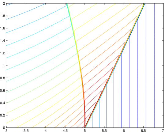
Refer to caption
Figure 4.8: Example 4.5: The contour of the rest energy density logarithm within the spacetime domain [3,7]×[t0,t0+2]37subscript𝑡0subscript𝑡02[3,7]\times[t_{0},t_{0}+2].

Fig. 4.8 gives the contour of the rest energy density logarithm within the spacetime domain [3,7]×[t0,t0+2]37subscript𝑡0subscript𝑡02[3,7]\times[t_{0},t_{0}+2]. Two relativistic shock waves are initially formed, and the stronger and straight moves to the right (the TOV region) while the weaker and curved propagates in the FRW-1 region. A expanding pocket of higher density is produced and then interacting with both FRW-1 and TOV metrics.
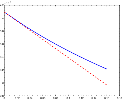
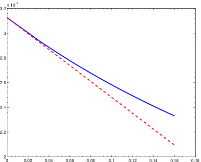
Refer to caption
Refer to caption
Figure 4.9: Example 4.5: Comparison of the reference (solid lines) and GRP solver based solutions (dash lines). The left and right are the first and the second components of 𝑼(t0+τ,r0)𝑼subscript𝑡0𝜏subscript𝑟0\mbox{\boldmath\small$U$}(t_{0}+\tau,r_{0}), respectively. The horizontal axis is the simulation time τ𝜏\tau.

Since this problem itself is GRP, it may be used to validate the accuracy of our GRP solver presented in Section 3.2.3. Fig. 4.9 gives a comparison of the GRP solver based solutions at the interface

𝑼GRP(t0+τ,r0)=𝑼RP+(𝑼t)GRPτ,superscript𝑼GRPsubscript𝑡0𝜏subscript𝑟0superscript𝑼RPsuperscript𝑼𝑡GRP𝜏{\mbox{\boldmath\small$U$}^{\mbox{\tiny GRP}}}({t_{0}}+\tau,r_{0})={\mbox{\boldmath\small$U$}^{\mbox{\tiny RP}}}+{\left({\frac{{\partial\mbox{\boldmath\small$U$}}}{{\partial t}}}\right)^{\mbox{\tiny GRP}}}\tau,

with the reference numerical solutions denoted by 𝑼REF(t0+τ,r0)superscript𝑼REFsubscript𝑡0𝜏subscript𝑟0\mbox{\boldmath\small$U$}^{\mbox{\tiny REF}}({t_{0}}+\tau,r_{0}), where 𝑼RPsuperscript𝑼RP{\mbox{\boldmath\small$U$}^{\mbox{\tiny RP}}} is the exact solution to the (classical) RP (3.7) with A=A(t0,r0),B=B(t0,r0)formulae-sequencesubscript𝐴𝐴subscript𝑡0subscript𝑟0subscript𝐵𝐵subscript𝑡0subscript𝑟0A_{*}=A(t_{0},r_{0}),B_{*}=B(t_{0},r_{0}), and the initial data 𝑼Lsubscript𝑼𝐿\mbox{\boldmath\small$U$}_{L} and 𝑼Rsubscript𝑼𝑅\mbox{\boldmath\small$U$}_{R} given by the left- and right-side limits at r=r0𝑟subscript𝑟0r=r_{0} of the initial data (4.8), and (𝑼/t)GRPsuperscript𝑼𝑡GRP{\left({{{\partial\mbox{\boldmath\small$U$}}}/{{\partial t}}}\right)^{\mbox{\tiny GRP}}} is computed by resolving the GRP at r=r0𝑟subscript𝑟0r=r_{0}. The reference solutions 𝑼REF(t0+τ,r0)superscript𝑼REFsubscript𝑡0𝜏subscript𝑟0\mbox{\boldmath\small$U$}^{\mbox{\tiny REF}}({t_{0}}+\tau,r_{0}) are computed by a second-order accurate MUSCL method with the Godunov flux on a very fine uniform mesh with the spatial step-size of 106superscript10610^{-6}. Table 4.4 lists the errors approximately evaluated by

eGRP(τ)=𝑼GRP(t0+τ,r0)𝑼REF(t0+τ,r0)2,subscript𝑒GRP𝜏subscriptnormsuperscript𝑼GRPsubscript𝑡0𝜏subscript𝑟0superscript𝑼REFsubscript𝑡0𝜏subscript𝑟02e_{\mbox{\tiny GRP}}(\tau)=\left\|\mbox{\boldmath\small$U$}^{\mbox{\tiny GRP}}({t_{0}}+\tau,r_{0})-\mbox{\boldmath\small$U$}^{\mbox{\tiny REF}}({t_{0}}+\tau,r_{0})\right\|_{2},

and corresponding convergence rates of the GRP solver. The results show that the GRP solver has second-order accuracy with respect to τ𝜏\tau and thus the accuracy of the limiting values (𝑼/t)GRPsuperscript𝑼𝑡GRP{\left({{{\partial\mbox{\boldmath\small$U$}}}/{{\partial t}}}\right)^{\mbox{\tiny GRP}}} is validated.

Table 4.4: Example 4.5: Numerical errors and corresponding convergence rates of the GRP solver based solution.
τ𝜏\tau 0.16 0.14 0.12 0.1 0.08 0.06 0.04 0.02
eGRP(τ)subscript𝑒GRP𝜏e_{\mbox{\tiny GRP}}(\tau) 3.42e-4 2.70e-4 2.04e-4 1.46e-4 9.67e-5 5.62e-5 2.59e-5 6.70e-6
order 1.78 1.80 1.83 1.86 1.88 1.92 1.95
Example 4.6 (Time reversal model)

The example considers reversing time and running the matched spacetime given in Example 4.5. For this purpose, the setup of this problem is the same as that for Example 4.5 except that the sign of the time is changed from positive to negative. In other words, the initial time for this test is t0=r0(1+v02)2v0subscript𝑡0subscript𝑟01superscriptsubscript𝑣022subscript𝑣0t_{0}=-\frac{r_{0}(1+v_{0}^{2})}{2v_{0}}.

Refer to caption
Figure 4.10: Same as Fig. 4.8, except for Example 4.6.
Refer to caption
Refer to caption
Figure 4.11: Same as Fig. 4.3, except for Example 4.6.
Refer to caption
Refer to caption
Figure 4.12: Same as Fig. 4.3, except for Example 4.6 and t=t0+0.6𝑡subscript𝑡00.6t=t_{0}+0.6.
Refer to caption
Refer to caption
Figure 4.13: Same as Fig. 4.3, except for Example 4.6 and t=t0+1𝑡subscript𝑡01t=t_{0}+1.

Fig. 4.10 gives the contour of the rest energy density logarithm within the spacetime domain [3,7]×[t0,t0+2]37subscript𝑡0subscript𝑡02[3,7]\times[t_{0},t_{0}+2] given by the GRP scheme with 400 uniform cells. From the initial discontinuity, two relativistic rarefaction waves are formed: a stronger wave moving to the left and connecting the FRW and TOV regions while a weaker propagating in the TOV region. A pocket of lower density is produced between the two rarefaction waves. Those are different from the forward time case in Example 4.5, where two shock waves are surrounding a region of higher density. Figs. 4.34.5 show the numerical solutions of the fluid variables at t=t0+0.2,t0+0.6𝑡subscript𝑡00.2subscript𝑡00.6t=t_{0}+0.2,~{}t_{0}+0.6, and t0+1subscript𝑡01t_{0}+1 by using the Godunov and GRP schemes with 400 uniform cells, respectively. We see that the results agree well with the reference solutions and the GRP scheme exhibits better resolution than the Godunov scheme. As the time increases, both the rarefaction waves and the pocket are expanding. At the left of this pocket, there is a density spike, growing and moving in the FRW region, and more matter is falling into the center of the universe as the time increase. If the more long time simulation is done, a black hole will be eventually produced [31].
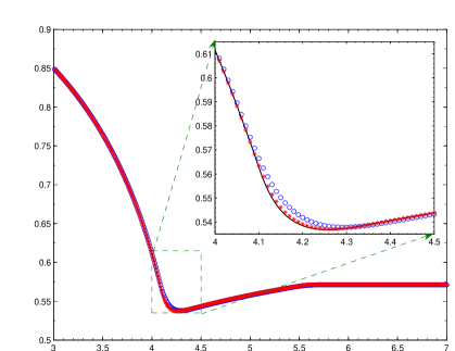
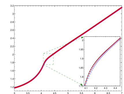
Refer to caption
Refer to caption
Figure 4.14: Same as Fig. 4.3, except for Example 4.6 and the metric functions A𝐴A (left) and B𝐵B (right) at t=t0+1𝑡subscript𝑡01t=t_{0}+1.
Refer to caption
Refer to caption
Figure 4.15: Same as Fig. 4.7, except for Example 4.6.

Figs. 4.14 and 4.15 display the numerical solutions and the corresponding errors in the metric functions A𝐴A and B𝐵B at t=t0+1𝑡subscript𝑡01t=t_{0}+1 by using the Godunov scheme and the GRP scheme with 400 uniform cells, respectively. These results show that the GRP scheme is much more accurate than the Godunov scheme, and the errors given by the GRP scheme is about ten percent of those computed by the Godunov scheme.
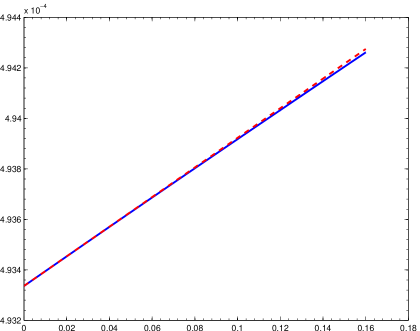
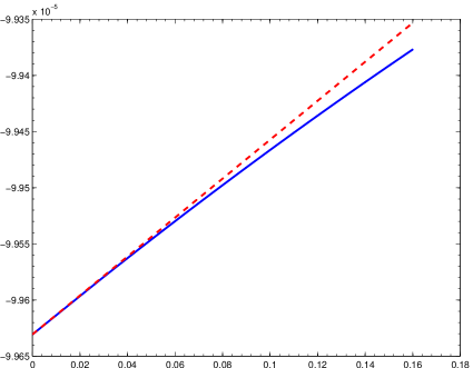
Refer to caption
Refer to caption
Figure 4.16: Same as Fig. 4.9, except for Example 4.6.
Table 4.5: Example 4.6: Numerical errors and corresponding convergence rates of the GRP solver based solution.
τ𝜏\tau 0.16 0.14 0.12 0.1 0.08 0.06 0.04
eGRP(τ)subscript𝑒GRP𝜏e_{\mbox{\tiny GRP}}(\tau) 2.74e-8 2.09e-8 1.53e-8 1.06e-8 6.75e-9 3.77e-9 1.66e-9
order 2.03 2.02 2.02 2.02 2.02 2.02

This reversing time problem is still a GRP. The GRP solver based solutions 𝑼GRP(t0+τ,r0)superscript𝑼GRPsubscript𝑡0𝜏subscript𝑟0\mbox{\boldmath\small$U$}^{\mbox{\tiny GRP}}({t_{0}}+\tau,r_{0}) are plotted in dash lines in Fig. 4.16 in comparison to the reference solutions given by a second-order accurate MUSCL method with the Godunov flux on a very fine uniform mesh with the spatial step-size of 106superscript10610^{-6}. The data in Table 4.5 show that second-order rates of convergence can be obtained for the proposed GRP solver and thus the accuracy of our GRP solver is validated.

5 Conclusions

The paper developed a second-order accurate direct Eulerian generalized Riemann problem (GRP) scheme for the spherically symmetric general relativistic hydrodynamical (RHD) equations and a second-order accurate discretization for the spherically symmetric Einstein (SSE) equations. Different from the resulting Godunov-type schemes based on exact or approximate Riemann solvers in general relativistic case, the GRP scheme could not be directly obtained by a local change of coordinates from the special relativistic case. In the GRP scheme, the Riemann invariants and the Runkine-Hugoniot jump conditions were directly used to analytically resolve the left and right nonlinear waves of the local GRP in the Eulerian formulation together with the local change of the metrics to obtain the limiting values of the time derivatives of the conservative variables along the cell interface and the numerical flux for the GRP scheme. Comparing to the GRP schemes for special RHDs [40], the derivation of the present GRP scheme is more technique. The energy-momentum tensor obtained in the GRP solver was utilized to evaluate the fluid variables in the SSE equations and the continuity of the metrics was constrained at the cell interfaces. Several numerical examples were presented to demonstrate the accuracy and effectiveness of the proposed GRP scheme, in comparison with the first-order accurate Godunov scheme.

Acknowledgements

This work was partially supported by the National Natural Science Foundation of China (Nos. 91330205 & 11421101).

Appendix A The Godunov scheme used in Section 4

Assume that the “initial” data at time tnsubscript𝑡𝑛t_{n} are

{𝑼h(tn,r)=𝑼jn,(Ah(tn,r)Bh(tn,r))=rj+12rΔr(Aj12nBj12n)+rrj12Δr(Aj+12nBj+12n),casessubscript𝑼subscript𝑡𝑛𝑟superscriptsubscript𝑼𝑗𝑛subscript𝐴subscript𝑡𝑛𝑟subscript𝐵subscript𝑡𝑛𝑟subscript𝑟𝑗12𝑟Δ𝑟superscriptsubscript𝐴𝑗12𝑛superscriptsubscript𝐵𝑗12𝑛𝑟subscript𝑟𝑗12Δ𝑟superscriptsubscript𝐴𝑗12𝑛superscriptsubscript𝐵𝑗12𝑛\left\{\begin{array}[]{l}\mbox{\boldmath\small$U$}_{h}(t_{n},r)=\mbox{\boldmath\small$U$}_{j}^{n},\\[8.53581pt] \left(\begin{array}[]{c}A_{h}(t_{n},r)\\ B_{h}(t_{n},r)\\ \end{array}\right)=\displaystyle{\frac{{r_{j+\frac{1}{2}}-r}}{{\Delta r}}}\left(\begin{array}[]{c}A_{j-\frac{1}{2}}^{n}\\ B_{j-\frac{1}{2}}^{n}\\ \end{array}\right)+\displaystyle{\frac{r-r_{j-\frac{1}{2}}}{\Delta r}}\left(\begin{array}[]{c}A_{j+\frac{1}{2}}^{n}\\ B_{j+\frac{1}{2}}^{n}\\ \end{array}\right),\end{array}\right.

for rIj𝑟subscript𝐼𝑗r\in I_{j}, where Ah(tn,r)subscript𝐴subscript𝑡𝑛𝑟A_{h}(t_{n},r) and Bh(tn,r)subscript𝐵subscript𝑡𝑛𝑟B_{h}(t_{n},r) are continuous at cell interface.

Step I. Evolve the solution 𝑼𝑼U at t=tn+1𝑡subscript𝑡𝑛1t=t_{n+1} of (2.7) by

𝑼jn+1=𝑼jnsuperscriptsubscript𝑼𝑗𝑛1superscriptsubscript𝑼𝑗𝑛\displaystyle\mbox{\boldmath\small$U$}_{j}^{n+1}=\mbox{\boldmath\small$U$}_{j}^{n} ΔtnΔr(Aj+12nBj+12n𝑭(𝑼j+12RP,n)Aj12nBj12n𝑭(𝑼j12RP,n))Δsubscript𝑡𝑛Δ𝑟superscriptsubscript𝐴𝑗12𝑛superscriptsubscript𝐵𝑗12𝑛𝑭superscriptsubscript𝑼𝑗12RP𝑛superscriptsubscript𝐴𝑗12𝑛superscriptsubscript𝐵𝑗12𝑛𝑭superscriptsubscript𝑼𝑗12RP𝑛\displaystyle-\displaystyle{\frac{{\Delta t_{n}}}{{\Delta r}}}\left({\sqrt{A_{j+\frac{1}{2}}^{n}B_{j+\frac{1}{2}}^{n}}\mbox{\boldmath\small$F$}\left(\mbox{\boldmath\small$U$}_{j+\frac{1}{2}}^{\mbox{\tiny RP},n}\right)-\sqrt{A_{j-\frac{1}{2}}^{n}B_{j-\frac{1}{2}}^{n}}\mbox{\boldmath\small$F$}\left(\mbox{\boldmath\small$U$}_{j-\frac{1}{2}}^{\mbox{\tiny RP},n}\right)}\right)
+Δtn𝑺(rj,Ajn,Bjn,𝑼jn),Δsubscript𝑡𝑛𝑺subscript𝑟𝑗superscriptsubscript𝐴𝑗𝑛superscriptsubscript𝐵𝑗𝑛superscriptsubscript𝑼𝑗𝑛\displaystyle+\Delta t_{n}\mbox{\boldmath\small$S$}\left({r_{j},A_{j}^{n},B_{j}^{n},\mbox{\boldmath\small$U$}_{j}^{n}}\right),

where Ajn:=12(Aj12n+Aj+12n),Bjn:=12(Bj12n+Bj+12n)formulae-sequenceassignsuperscriptsubscript𝐴𝑗𝑛12superscriptsubscript𝐴𝑗12𝑛superscriptsubscript𝐴𝑗12𝑛assignsuperscriptsubscript𝐵𝑗𝑛12superscriptsubscript𝐵𝑗12𝑛superscriptsubscript𝐵𝑗12𝑛A_{j}^{n}:=\frac{1}{2}\left(A_{j-\frac{1}{2}}^{n}+A_{j+\frac{1}{2}}^{n}\right),B_{j}^{n}:=\frac{1}{2}\left(B_{j-\frac{1}{2}}^{n}+B_{j+\frac{1}{2}}^{n}\right), and 𝑼j+12RP,nsuperscriptsubscript𝑼𝑗12RP𝑛\mbox{\boldmath\small$U$}_{j+\frac{1}{2}}^{\mbox{\tiny RP},n} is the value at r=rj+12𝑟subscript𝑟𝑗12r=r_{j+\frac{1}{2}} of the exact solution to the following RP

{𝑼t+Aj+12nBj+12n𝑭(𝑼)r=0,r>0,t>tn,𝑼(tn,r)={𝑼jn,r<rj+12,𝑼j+1n,r>rj+12,casesformulae-sequence𝑼𝑡superscriptsubscript𝐴𝑗12𝑛superscriptsubscript𝐵𝑗12𝑛𝑭𝑼𝑟0formulae-sequence𝑟0𝑡subscript𝑡𝑛otherwise𝑼subscript𝑡𝑛𝑟casessuperscriptsubscript𝑼𝑗𝑛𝑟subscript𝑟𝑗12superscriptsubscript𝑼𝑗1𝑛𝑟subscript𝑟𝑗12otherwise\begin{cases}\displaystyle{\frac{{\partial\mbox{\boldmath\small$U$}}}{{\partial t}}}+\sqrt{A_{j+\frac{1}{2}}^{n}B_{j+\frac{1}{2}}^{n}}\displaystyle{\frac{{\partial\mbox{\boldmath\small$F$}(\mbox{\boldmath\small$U$})}}{{\partial r}}}=0,\qquad r>0,~{}t>t_{n},\\[8.53581pt] \mbox{\boldmath\small$U$}(t_{n},r)=\begin{cases}\mbox{\boldmath\small$U$}_{j}^{n},&r<r_{j+\frac{1}{2}},\\ \mbox{\boldmath\small$U$}_{j+1}^{n},&r>r_{j+\frac{1}{2}},\end{cases}\end{cases}

Step II. Calculate Aj+12n+1superscriptsubscript𝐴𝑗12𝑛1A_{j+\frac{1}{2}}^{n+1} and Bj+12n+1superscriptsubscript𝐵𝑗12𝑛1B_{j+\frac{1}{2}}^{n+1}, following Step V of the GRP scheme in Section 3.1.

References

  • [1] M. Ben-Artzi and J. Falcovitz, A second-order Godunov-type scheme for compressible fluid dynamics, J. Comput. Phys., 55 (1984), 1-32.
  • [2] M. Ben-Artzi and J. Falcovitz, Generalized Riemann Problems in Computational Fluid Dynamics, Cambridge University Press, 2003.
  • [3] M. Ben-Artzi and J.Q. Li, Hyperbolic balance laws: Riemann invariants and the generalized Riemann problem, Numer. Math., 106 (2007), 369-425.
  • [4] M. Ben-Artzi, J.Q. Li, and G. Warnecke, A direct Eulerian GRP scheme for compressible fluid flows, J. Comput. Phys., 218 (2006), 19-43.
  • [5] J.A. Font, Numerical hydrodynamics and magnetohydrodynamics in general relativity, Living Rev. Relativity, 11 (2008), 7.
  • [6] E. Gourgoulhon, Simple equations for general relativistic hydrodynamics in spherical symmetry applied to neutron star collapse, Astron. Astrophys., 252 (1991), 651-663.
  • [7] J. Groah, J. Smoller, and B.Temple, Shock wave interactions in general relativity, Springer Monographs in Mathematics, Springer, New York, 2007.
  • [8] F.S. Guzmán, F.D. Lora-Clavijo, and M.D. Morales, Revisiting spherically symmetric relativistic hydrodynamics, Rev. Mex. Fis. E, 58 (2012), 84-98.
  • [9] E. Han, J.Q. Li, and H.Z. Tang, An adaptive GRP scheme for compressible fluid flows, J. Comput. Phys., 229 (2010), 1448-1466.
  • [10] E. Han, J.Q. Li, and H.Z. Tang, Accuracy of the adaptive GRP scheme and the simulation of 2-D Riemann problems for compressible Euler equations, Commun. Comput. Phys., 10 (2011), 577-606.
  • [11] L.D. Landau and E.M. Lifschitz, Fluid Meshanics, Pergaman Press, 1987.
  • [12] J.Q. Li and G.X. Chen, The generalized Riemann problem method for the shallow water equations with bottom topography, Int. J. Numer. Meth. in Eng., 65 (2006), 834-862.
  • [13] J.Q. Li, Q.B. Li, and K. Xu, Comparisons of the generalized Riemann solver and the gas-kinetic scheme for inviscid compressible flow simulations, J. Comput. Phys., 230 (2011), 5080-5099.
  • [14] J.Q. Li, T.G. Liu, and Z.F. Sun, Implementation of the GRP scheme for computing radially symmetric compressible fluid flows, J. Comput. Phys., 228 (2009), 5867-5887.
  • [15] T. Li and W.C. Yu, Boundary Value Problem for Quasilinear Hyperbolic Systems, Mathematics Department, Duke University, 1985.
  • [16] J.Q. Li and Y.J. Zhang, The adaptive GRP scheme for compressible fluid flows over unstructured meshes, J. Comput. Phys., 242 (2013), 367-386.
  • [17] M. Liebendöerfer, S. Rosswog, and F.-K. Thielemann, An adaptive grid, implicit code for spherically symmetric, general relativistic hydrodynamics in comoving coordinates, Astrophys. J. Suppl., 141 (2002), 229-246.
  • [18] M. Liebendörfer, O.E.B. Messer, A. Mezzacappa, S.W. Bruenn, C.Y. Cardall, and F.K. Thielemann, A Finite difference representation of neutrino radiation hydrodynamics for spherically symmetric general relativistic supernova simulations, Astrophys. J. Suppl., 150 (2004), 263-316.
  • [19] J.M. Martí and E. Müller, Numerical hydrodynamics in special relativity, Living Rev. Relativity, 6 (2003), 7.
  • [20] M.M. May and R.H. White, Hydrodynamic calculations of general relativistic collapse, Phys. Rev. D, 141 (1996), 1232-1241.
  • [21] M.M. May and R.H. White, Stellar dynamics and gravitational collapse, Methods Comput. Phys., 7 (1967), 219-258.
  • [22] E. O’Connor and C.D. Ott, A new open-source code for spherically symmetric stellar collapse to neutron stars and black holes, Class. Quantum Grav., 27 (2010), 114103.
  • [23] D.H. Park, I. Cho, G. Kang, and H.M. Lee, A fully general relativistic numerical simulation code for spherically symmetric matter, J. Korean Phys. Soc., 62 (2013), 393-405.
  • [24] J.A. Pons, J.A. Font, J.M. Ibáñez, J.M. Martí, and J.A. Miralles, General relativistic hydrodynamics with special relativistic Riemann solvers, Astron. Astrophys., 339 (1998), 638-642.
  • [25] J.Z. Qian, J.Q. Li, and S.H. Wang, The generalized Riemann problems for compressible fluid flows: Towards high order, J. Comput. Phys., 259 (2014), 358-389.
  • [26] D. Radice and L. Rezzolla, Discontinuous Galerkin methods for general-relativistic hydrodynamics: Formulation and application to spherically symmetric spacetimes, Phys. Rev. D., 84 (2011), 024010.
  • [27] J.V. Romero, J.M. Ibáñez, J.M. Martí, andJ.A. Miralles, A new spherically symmetric general relativistic hydrodynamical code, Astrophys. J, 46 (1996), 839-854.
  • [28] J. Smoller and B. Temple, Global solutions of the relativistic Euler equations, Comm. Math. Phys., 157 (1993), 67-99.
  • [29] H.Z. Tang and T. Tang, Adaptive mesh methods for one- and two-dimensional hyperbolic conservation laws, SIAM J. Numer. Anal., 41 (2003), 487-515.
  • [30] B. Temple and J. Smoller, Expanding wave solutions of the Einstein equations that induce an anomalous acceleration into the Standard Model of Cosmology, Proc. Natl Acad. Sci., 106 (2009), 14213-14218.
  • [31] Z. Vogler, The numerical simulation of general relativistic shock waves by a locally inertial Godunov method featuring dynamic time dilation, Ph.D. thesis, University of California, 2010.
  • [32] Z. Vogler and B. Temple, Simulation of general relativistic shock wave interactions by a locally inertial Godunov method featuring dynamical time dilation, Proc. R. Soc. A, 468 (2012), 1865-1883.
  • [33] J.R. Wilson, Numerical study of fluid flow in a Kerr space, Astrophys. J., 173 (1972), 431-438.
  • [34] J.R. Wilson and G.J. Mathews, Relativistic Numerical Hydrodynamics, Cambridge University Press, 2003.
  • [35] K.L. Wu and H.Z. Tang, Finite volume local evolution galerkin method for two-dimensional relativistic hydrodynamics, J. Comput. Phys., 256 (2014), 277-307.
  • [36] K.L. Wu and H.Z. Tang, High-order accurate physical-constraints-preserving finite difference WENO schemes for special relativistic hydrodynamics, J. Comput. Phys., 298 (2015), 539-564.
  • [37] K.L. Wu, Z.C. Yang, and H.Z. Tang, A third-order accurate direct Eulerian GRP scheme for the Euler equations in gas dynamics, J. Comput. Phys., 264 (2014), 177-208.
  • [38] K.L. Wu, Z.C. Yang, and H.Z. Tang, A third-order accurate direct Eulerian GRP scheme for one-dimensional relativistic hydrodynamics, East Asian J. Appl. Math., 4 (2014), 95-131.
  • [39] S. Yamada, An implicit Lagrangian code for spherically symmetric general relativistic hydrodynamics with an approximate Riemann solver, Astrophys. J., 475 (1997), 720-739.
  • [40] Z.C. Yang, P. He, and H.Z. Tang, A direct Eulerian GRP scheme for relativistic hydrodynamics: One-dimensional case, J. Comput. Phys., 230 (2011), 7964-7987.
  • [41] Z.C. Yang and H.Z. Tang, A direct Eulerian GRP scheme for relativistic hydrodynamics: Two-dimensional case, J. Comput. Phys., 231 (2012), 2116-2139.