Distant IE by Bootstrapping Using Lists and Document Structure
Abstract
Distant labeling for information extraction (IE) suffers from noisy training data. We describe a way of reducing the noise associated with distant IE by identifying coupling constraints between potential instance labels. As one example of coupling, items in a list are likely to have the same label. A second example of coupling comes from analysis of document structure: in some corpora, sections can be identified such that items in the same section are likely to have the same label. Such sections do not exist in all corpora, but we show that augmenting a large corpus with coupling constraints from even a small, well-structured corpus can improve performance substantially, doubling F1 on one task.
Introduction
In distantly-supervised information extraction (IE), a knowledge base (KB) of relation or concept instances is used to train an IE system. For instance, a set of facts like adverseEffectOf(meloxicam, stomachBleeding), interactsWith(meloxicam, ibuprofen), might be matched against a corpus, and the matching sentences then used to generate training data consisting of labeled entity mentions. For instance, matching the KB above might lead to labeling passage 1 from Table 1 as support for the fact adverseEffectOf(meloxicam, stomachBleeding).
A weakness of distant supervision is that it produces noisy training data, when matching errors occur. E.g., consider using distant learning to classify noun phrases (NPs) into types, like drug or symptom; matching a polysemous term like weakness could lead to incorrectly-labeled mention examples. Hence distant supervision is often coupled with learning methods that allow for this sort of noise by introducing latent variables for each entity mention (e.g., (?; ?; ?)); by carefully selecting the entity mentions from contexts likely to include specific KB facts (?); or by careful filtering of the KB strings used as seeds (?).
-
1.
“Avoid drinking alcohol. It may increase your risk of stomach bleeding.”
-
2.
“Get emergency medical help if you have chest pain, weakness, shortness of breath, slurred speech, or problems with vision or balance.”
-
3.
“Check the label to see if a medicine contains an NSAID (non-steroidal anti-inflammatory drug) such as aspirin, ibuprofen, ketoprofen, or naproxen.”
We describe a way of reducing the noise associated with distant IE by identifying coupling constraints between potential instance labels. As one example of coupling, NPs in a conjunctive list are likely to have the same category, a fact used in prior work (?) to propagate NP categories from unambiguous NPs (such as chest pain in passage 2) to ambiguous ones (e.g., the mention weakness in the same passage). Bing et al. used propagation methods (?; ?) to exploit this intuition, by propagating the low-confidence labels associated with distance supervision matches through an appropriate graph.

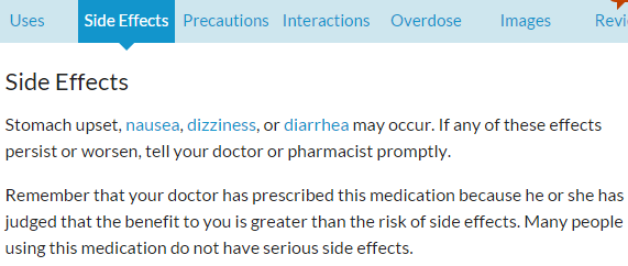
In this paper we adapt this coupling to extracting relations, rather than NP categories. We also explore additional types of coupling, derived from analysis of document structure. In particular, in some corpora, sections can be identified that correspond fairly accurately to relation arguments. For example, Figure 1 shows part of a small but well-structured corpus (discussed below) which contains sections labeled “Side Effects”. This document structure cannot be used to directly derive training data (there are many NPs of many types, such as “doctor” or “physicial”, even in a “Side Effects” section), nevertheless, we will show that coupling schemes can be derived and used to improve distantly-supervised IE, even when the test corpus does not contain well-structured sections.
DIEBOLDS: Distant IE by BOotstrapping using List and Document Structure
Here we describe a pipelined system called DIEBOLDS. DIEBOLDS parses two corpora: a large target corpus and a smaller structured corpus, and also perfoms some document analysis on the structured corpus. It then extracts NP chunks, together with features that describe each NP mention, as well as coupling information of various types. In particular, DIEBOLDS derives edges that define list coupling, section coupling, and neighbor coupling. DIEBOLDS then creates an appropriate graph, and uses distant supervision, in combination with a label-propagation method, to find mentions that can be confidently labeled. From this pseudo-labeled data, it uses ordinary classifier learners to classify NP mentions by relation types, where the relation indicates the relationship of an NP mention to the entity that is the subject of the document containing the mention. Extensive experiments are conducted on two corpora, for diseases and drugs, and the results show that this approach significantly improves over a classical distant-supervision approach. The architecture of the system is shown in Figure 2.
Knowledge Base and Corpora
Distantly-supervised IE is often used to extend an incomplete KB. Even large curated KBs are often incomplete: e.g., a recent work showed that more than 57% of the nine commonly used attribute/relation values are missing for the top 100k most frequent PERSON entities in Freebase (?). We consider extending the coverage of Freebase in the medical domain, which is currently fairly limited: e.g., a Freebase snapshot from April 2014 has (after filtering noise with simple rules such as length greater than 60 characters and containing comma) only 4,605 instances in “Disease or Medical Condition“ type and 4,383 instances in “Drug” type, whereas dailymed.nlm.nih.gov contains data on over 74k drugs, and malacards.org lists nearly 10k diseases.
We focus on extracting instances for 8 relations, defined in Freebase, of drugs and diseases. The targeted drug relations include used_to_treat, conditions_this_may_prevent, and side_effects. The targeted disease relations include treatments, symptoms, risk_factors, causes, and prevention_factors.
Our target drug corpus, called DailyMed, is downloaded from dailymed.nlm.nih.gov which contains 28,590 XML documents, each of which describes a drug that can be legally prescribed in the United States. Our target disease corpus, called WikiDisease, is extracted from a Wikipedia dump of May 2015 and it contains 8,596 disease articles. Large amount of this information in our corpora is in free text. DailyMed includes information about treated diseases, adverse effects, drug ingredients, etc. WikiDisease includes information about causes, treatments, symptoms, etc.
Our corpora are “entity centric”, i.e., each document discusses a single drug or disease. Relation extraction is to predict the type of an entity mention and its relation with the document subject. For instance, the mention chest pain is an instance of side_effects of the drug meloxicam in Table 1.
The structured drug corpus, called WebMD, is collected from www.webmd.com, and each drug page has 7 sections, such as Uses, Side Effects, Precautions, etc. WebMD contains 2,096 pages. The structured disease corpus, called MayoClinic, is collected from www.mayoclinic.org. The sections of MayoClinic pages include Symptoms, Causes, Risk Factors, Treatments and Drugs, Prevention, etc. MayoClinic contains 1,117 pages. These sections discuss the important aspects of drugs and diseases, and Freebase has corresponding relations to capture such aspects.
Propagation Graph
List Extraction and Graph with List Edges
We use the GDep parser (?), a dependency parser trained on the GENIA Treebank, to parse the corpora. We use a simple POS-tag based noun-phrase (NP) chunker, and extract a list for each coordinating conjunction that modifies a nominal. For each NP we extract features (described below); and for each identified coordinate-term list, we extract its items.
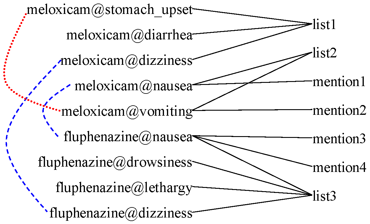
The extracted lists and their items, as well as entity mentions and their corresponding NPs, are used to create bipartite graph. One set of vertices correspond to entity mentions, where each mention is encoded as a pair, consisting of the subject entity for the document, paired with the string corresponding to the NP itself. The other set of vertex identifiers are for the lists. A mention not inside a list is regarded as a singleton list that contains only one item. If an NP is contained by a list, an edge between the NP vertex and the list vertex is included in the graph. We refer to such edges as list edges (L-edges for short). An example bipartite graph is given in Figure 3 (ignore for now the dashed and dotted links). There are 9 instances of side_effects relations from three lists and four mentions extracted from two drugs.
Section Edges
For each subject entity, there are only a few pages (typically one) that discuss that entity. Hence a graph containing only list edges is not well-connected: generally the edges only link vertices from a single document. To improve the connectivity, we augment the graph of a target corpus with a graph derived from the structured corpus, thus building an augmented graph.
Firstly, a bipartite graph for a structured corpus is constructed. In addition to lists, we employ the section information of the structured documents: specifically, edges are added between the drug-NP pairs (or disease-NP pairs) as exemplified by the dotted and dashed links in Figure 3. We add a dashed blue edge for two drug-NP pairs if their NP strings match and the two NPs come from the same section of two documents. In Figure 3, two such edges are added because of the same section “Side Effects” in two drug documents, i.e., meloxicam and fluphenazine. The intuition is that if an NP appears in the same section of different documents, the occurrences are very likely to have the same relation with the corresponding document subjects. Also, if two NPs appear in the same section of a document, they might have the same relation with the document subject. For instance, both “vomiting” and “stomach_upset” appear in “Side Effects” section of meloxicam, it is reasonable to infer they might have the same relation label. We refer to those edges as section edges (S-edges).
Our target corpora have thousands of different section titles, many of which are not related in any way to the relations being extracted, so we do not add S-edges for their sections. Now we augment the bipartite graph of a target corpus with the graph for a corresponding structured corpus.
Neighbor Edges
We might want to further link the drug-NP (or disease-NP) pairs of a target corpus and a structured corpus with similarity-based edges. We add a weighted edge for two drug-NP pairs if their NP mentions are similar, where the weight is in and calculated with TFIDF-weighted BOW of contexts for the NPs. The context contains all words, excluding NP itself, from sentences containing the NP. We weight these edges with the cosine similarity of the two BOW objects, after TFIDF weighting. (Note that that the weight of other edges is 1.) Such weighted edges capture the intuition that if two NPs have similar contexts, they are very likely to have the same relation label. We refer to such edge as near-neighbor edges (N-edges).
Obviously, if both drug names and NP strings in two drug-NP pairs match, they are merged as the same node in the augmented graph. For NP string and drug/disease name matching, we employ SecondString with SoftTFIDF as distance metric (?) and the match threshold is 0.8. It is also used for all baselines compared in the Experiments section.
Label Propagation
Considering the nature of those added edges, it seems plausible to use label propagation on the above graph to propagate relation types from seed drug-NP (disease-NP) pairs with known relation types, e.g., those matching the triples in KB, to more pairs and lists across the graph.
This can be viewed as semi-supervised learning (SSL) of the pairs that may denote a relation (e.g., “used_to_treat” or “side_effects”). We adopt an existing multi-class label propagation method, namely, MultiRankWalk (MRW) (?), to handle our task, which is a graph-based SSL related to personalized PageRank (PPR) (?) (aka random walk with restart (?)). Given a graph represented by matrix , a vector probability distribution over the nodes is found that satisfies the equation
where , is the column-stochastic transition matrix of the graph; and , the seed vector, is a uniform distribution over the labeled training instances of each class (here the facts from KB); and is the restart probability. (In the experiments we use .) The vector can be interpreted as the probability distribution of a random walk on the graph, where at each step there is a probability to “teleport” to a random node with distribution . MRW performs one such computation of a vector for each class , then assigns each instance to the class with highest score, i.e. it predicts for the label .
MRW can be viewed as simply computing one personalized PageRank vector for each class, where each vector is computed using a personalization vector that is uniform over the seeds, and finally assigning to each node the class associated with its highest-scoring vector. MRW’s final scores depend on centrality of nodes, as well as proximity to the seeds, and in this respect MRW differs from other label propagation methods (e.g., (?)): in particular, it will not assign identical scores to all seed examples. Hence MRW will weight up seeds that are well-connected to other seeds, and weight down seeds that are in“outlying” sections of the graph. The MRW implementation we use is based on ProPPR (?).
Classification
One could imagine using the output of MRW to extend a KB directly. However, the process described above cannot be used conveniently to label new documents as they appear. Since this is also frequently a goal, we use the MRW output to train a classifier, which can be then used to classify the entity mentions (singleton lists) and coordinate lists in any new document, as well as those not reached ones in the above graph.
We use the same feature generator for both mentions and lists. Shallow features include: tokens in the NPs, and character prefixes/suffixes of these tokens; tokens from the sentence containing the NP; and tokens and bigrams from a window around the NPs. From the dependency parsing, we also find the verb which is the closest ancestor of the head of the NP, all modifiers of this verb, and the path to this verb. For a list, the dependency features are computed relative to the head of the list.
We used an SVM classifier (?) and discard singleton features, and also the most frequent 5% of all features (as a stop-wording variant). We train a binary classifier on the top N lists (including mentions and coordinate lists) of each relation, as scored by MRW. A linear kernel and defaults for all other parameters are used. If a new list or mention is not classified as positive by all binary classifiers, it is predicted as “other”.
Parameter Tuning
Two important parameters in DIEBOLDS are the seed number for label propagation with MRW and the top N number for generating training examples of SVM. Here we describe our method for tuning them. The evaluation data is generated with a validating set of facts. Specifically, these facts are used as seeds for MRW and the top 200 lists (singleton and coordinate lists) of each relation, as scored by MRW, are collected. We regard these lists as pseudo-labeled examples to test the performance of trained classifiers in DIEBOLDS. Their feature vectors are generated in the same way as above. We refer to total available seeds for DIEBOLDS as development set, no overlapping with the validating set here.
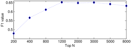
The effect of top N number when using 100% of development seeds is given in Figure 4. As we expected, too few examples or too many examples are not effective for training an accurate classifier. The reason is that, if the examples are too few, they are not adequate to train a classifier with good generalization capability. One the other hand, if N is too large, the quality of the involved examples cannot be guaranteed, which also degrades the accuracy of the trained classifier. A good aspect can be observed from Figure 4 is that the classifier’s performance is quite stable in a large N range, from 1,200 to 5,000. It indicates that DIEBOLDS is quite robust and its classification performance is not very sensitive to this parameter.
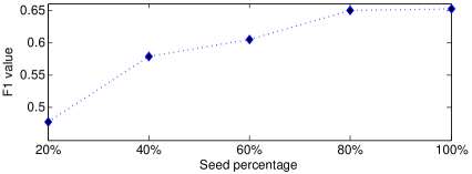
We also try different ratios of the development set as seeds of label propagation in DIEBOLDS. The results are given in Figure 5. When the seed number is mall, say 20%, the trained classifier is not effective. As the seed number increasing, F1 value gets improved. The values of 80% and 100% are quite similar, and it shows a certain number of seeds will almost achieve the best result, and the marginal improvement with more seeds is limited. It is because the label propagation with MRW helps collect sufficiently good training examples with less number of seeds, (i.e. 80%).
Experiments
Evaluation Datasets 111We released some data at http://www.wcohen.com.
For the first dataset, we manually labeled 10 pages from WikiDisease corpus and 10 pages from DailyMed corpus. The annotated text fragments are those NPs that are object values of those 8 relations, with the drug or disease described by the corresponding document as the relation subject. In total, we collected 436 triple facts for disease domain and 320 triples facts for drug domain. A pipeline’s task is to extract the objects of the relations in a given document.
For the second dataset, we employ questions in the training dataset of BioASQ3-Task B 222http://participants-area.bioasq.org/general_information/Task3b/ to examine the ability of DIEBOLDS output on answering those questions. This dataset contains four types of questions: yes/no questions, factoid questions, list questions, and summary questions (?). We focus on factoid and list questions because these questions require a particular entity name (e.g., of a disease, drug, or gene), or a list of them as an answer. We only keep the questions that are related to the relations in this paper, and finally we get 58 questions, including 37 factoid questions and 21 list questions. Each natural language question is translated to a structured database query, which can be evaluated on any KB. For instance, the answer of query(treatsDisease, daonil, Y) is expected to be a disease name, i.e. “diabetes mellitus”.
Baselines
The first two baselines are distant-supervision-based. A DS baseline attempts to classify each NP in its input corpus into one of the interested relation types or “other” with the training seeds as distance supervision. Each sentence in the corpus is processed with the same preprocessing pipeline to detect NPs. Then, these NPs are labeled with the training seeds. The features are defined and extracted in the same way as we did for DIEBOLDS, and binary classifiers are trained with the same method. The first DS baseline only generates labeled examples from the target corpus, and it is named DS1. While the second DS baseline uses both target corpus and structured corpus, and it is named DS2. The third baseline applies list structure into DS1, and it first preforms label propagation with MRW on the bipartite graph of target corpus. Then binary classifiers are trained with the top N lists scored by MRW in the same way. This baseline is named DS+L.
Variants of DIEBOLDS
We also investigate different variants of DIEBOLDS. The first variant removes S-edges and N-edges from the graph of DIEBOLDS when propagating labels, and it is named DIEBOLDS-SN. By removing S-edges and N-edgess respectively, we have two more variants, named DIEBOLDS-S and DIEBOLDS-N. We use the same way to tune the parameters for these variants and also the baseline DS+L. Specifically, all baselines and variants employ 100% of the training seeds, and top N values are determined as the ones achieved the best performance on the tuning examples.
Experimental Settings
We extracted triples of these 8 target relations from Freebase. Specifically, if the subject of a triple matches with a drug or disease name in our target corpora and its object value also appear in that document, it is extracted as a seed. For disease domain, we get 1,524, 1,976, 593, 674, and 99 triples for treatments, symptoms, risk_factors, causes, and prevention_factors, respectively. For drug domain, we get 2,973, 229, and 243 triples for used_to_treat, conditions_his_may_prevent, and side_effects, respectively. These triples are split into development set and validating set in the ratio of 9:1. The development set is used as seed of MRW, and the validating set is used to validate different parameters.
Note that we did not use the seeds that only match with the structured corpora, because we aim at examining the effect of using structured corpora on the extraction of target corpus and excluding such seeds will avoid the bias because of more seeds. We report the average performance of 3 runs, and each run has its own randomly generated development set and validating set to avoid the bias of seed sampling,
Results on Labeled Pages
DS+L and DIEBOLDS variants can classify both NPs and coordinate lists. After that, lists are broken into items, i.e. NPs, for evaluation. We evaluate the performance of different pipelines from IR perspective, with a subject (i.e., document name) and a relation together as a query, and extracted NPs as retrieval results. Thus, we have 50 and 30 queries for disease domain and drug domain, respectively. The predicted probability by the binary classifiers serves as the ranking score inside each query.
| Disease | Drug | |||||
| P | R | F1 | P | R | F1 | |
| DS1 | 0.117 | 0.350 | 0.175 | 0.020 | 0.268 | 0.037 |
| DS2 | 0.115 | 0.361 | 0.174 | 0.018 | 0.254 | 0.034 |
| DS+L | 0.122 | 0.380 | 0.184 | 0.031 | 0.432 | 0.057 |
| Freebase | 0.202 | 0.037 | 0.062 | 0.318 | 0.022 | 0.041 |
| DIEBOLDS-SN | 0.128 | 0.374 | 0.191 | 0.045 | 0.451 | 0.082 |
| DIEBOLDS-S | 0.136 | 0.382 | 0.198 | 0.048 | 0.480 | 0.088 |
| DIEBOLDS-N | 0.131 | 0.372 | 0.194 | 0.047 | 0.419 | 0.085 |
| DIEBOLDS | 0.143 | 0.372 | 0.209 | 0.050 | 0.435 | 0.090 |
The results evaluated by precision, recall and F1 measure are given in Table 2. DIEBOLDS and its variants outperform the baselines in all metrics. DIEBOLDS is the most effective pipeline in both domains, and its improvement over DS1, pure distant supervision, on F1 is about 20% in disease domain, and more than 100% in drug domain.
The precision of DIEBOLDS is consistently better than its variants. Presumably, this is true because as more linking information is added into the graph, the top-scored lists or NPs in MRW are becoming less noisy. DIEBOLDS-S achieves the best recall values in both domains. By removing the S-edges from DIEBOLDS, N-edges become more important in the graph and MRW walks to more diverse NPs and lists. Thus, the trained classifier has better generalization capability and achieves better recall values. On the other hand, its precision is affected. DIEBOLDS-SN outperforms DS+L under most metrics in both domains. Both of them explore list information in label propagation, but the difference is that DIEBOLDS-SN employs a merged graph of target corpus and structured corpus. Thus, the lists from structured corpus enhances the transduction capability of the graph.
The performance order of different pipelines is very stable. The more information of list and document structure is used, the better the performance is. It shows that these types of information are all value-added and combining them is a workable way to get better results. Without using the structured corpus, DS+L still achieves encouraging improvements over DS1 list is a useful resource by itself. One interesting observation is that although DS2 also uses the distantly labeled examples in the structured corpus, its performance is similar or even worse than DS1. It shows that simply adding some examples from another corpus is not an effective approach to upgrade the performance. The results in drug domain are much lower than those of disease domain. The main reason is that documents of DailyMed are usually quite long, and too much description of different aspects of a drug overwhelms the targeted facts.
We also employ Freebase as a comparison system, and use its facts as the system output. It is not unexpected to observe very low recall values in both domains, since the coverage of Freebase on specific domains such as biomedical domain is limited. Specifically, Freebase only contains 16 disease triples and 7 drug triples of those annotated ones. However, the precision values are also not quite high, especially for disease domain. The reason is two-fold. First, our labeled pages do not contain all facts of those relations, but Freebase does contain some facts of those missing ones from the labeled pages. The second reason is that Freebase is not noise-free, and some facts in it are actually wrong.
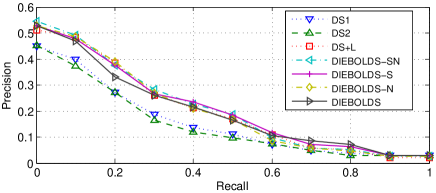
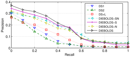
The precision-recall curves are given in Figures 6 and 7. We adopt the 11-point curve which is a graph plotting the interpolated precision of an IR system at 11 standard recall levels (?). In general, the top ranked results are of reasonable accuracy. For the top results, the average precision values of DIEBOLDS are about 0.5 and 0.35. DIEBOLDS and its variants are better than the baselines.
Results on BioASQ Questions
To answer some queries in BioASQ dataset, the facts from different relations need to
be combined. For example, to answer query(treatsDiseaseWithSideEffect, X , epilepsy,
spina_bifida), the triples of used_to_treat and side_effect_of are combined in:
query(treatsDiseaseWithSideEffect, Drug, Disease, Effect)
:- used_to_treat(Drug, Disease), side_effect_of(Effect, Drug)
We define such rules together with the triples as input of ProPPR 333https://github.com/TeamCohen/ProPPR,
to answer these queries.
We compare the triples of Freebase and DIEBOLDS pipeline. (Output of DIEBOLDS only comes from the target corpora.) The evaluation metrics are Mean Average Precision (MAP) and Mean Reciprocal Rank (MRR), commonly used for question answering, as well as Recall. The results are given in Table 3. of Freebase. It shows the higher scored triples from DIEBOLDS have reasonably good accuracy. On the other hand, Freebase does not have The recall value of DIEBOLDS is about 80% higher than that of Freebase. It shows that DIEBOLDS returns richer knowledge.
| MRR | MAP | Recall | |
|---|---|---|---|
| DIEBOLDS | 0.094 | 0.092 | 0.195 |
| Freebase | 0.025 | 0.025 | 0.109 |
Related Work
Distant supervision was initially employed by ? (?) in the biomedical domain under a different terminology, i.e. weakly labeled data. Then, it attracted attentions from the IE community. ? (?) employed Freebase to label sentences containing a pair of entities that participate in a known Freebase relation, and aggregated the features from different sentences for this relation. ? (?; ?) also proposed an entity-centric corpus oriented method, and employed infoboxes to label their corresponding Wikipedia articles. DIEBOLDS employs Freebase to label entity-centric documents of particular domains.
To tolerate the noise in distantly-labeled examples, ? (?) assumed that at least one of the relation mentions in each “bag” of mentions sharing a pair of argument entities which bears a relation, expresses the target relation, instead of taking all of them as correct examples. MultiR (?) and Multi-Instance Multi-Label Learning (MIML) (?) further improve it to support multiple relations expressed by different sentences in a bag. Different from them, before feeding the noisy examples into a learner, DIEBOLDS improves the quality of training data with a bootstrapping step, which propagates the labels in an appropriate graph. The benefit of this step is two-fold. First, it distills the distantly-labeled examples by propagating labels through those coupling edges, and downweights the noisy ones. Second, the propagation will walk to other good examples that are not distantly labeled with the seeds. In the classic bootstrapping learning (?; ?; ?), small number of seed instances are used to extract, from a large corpus, new patterns, which are used to extract more instances. Then new instances are used to extract more patterns, in an iterative fashion. DIEBOLDS departs from earlier bootstrapping uses in combining label propagation with a standard classification learner, so that it can improve the quality of distant examples and collect new examples simultaneously.
Conclusions and Future Work
We explored an alternative approach to distant supervision by detection of lists in text and utilization of document structure to overcome the weakness of distant supervision becaseu of noisy training data. It uses distant supervision and label propagation to find mentions that can be confidently labeled, and uses them to train classifiers to label more entity mentions. The experimental results show that this approach consistently and significantly outperforms naive distant-supervision approaches.
For future work, one direction is to build more comprehensive graph by integrating corpora from highly related domains. Another worthwhile direction is to suppress the false positives, which will significantly upgrade the overall performance. Another approach that might be able to upgrade the performance is to use an annotated validating page set, instead of using 10% Freebase seeds to automatically generate testing examples, for tuning parameters. DIEBOLDS-SN outperforms DS+L by using the additional list information from the structured corpus. This reminds us that using more list information of other corpora, which could be general corpora and much larger than the target corpus, might be a worthwhile approach to try for enhancing the extraction on the target corpus. One might want to directly classify the drug-NP pairs on the left side of the graph, instead of lists and mentions. This approach aggregates different mention occurrences of the same NP, falling in the macro-reading paradigm (?), and it might also be a good direction to explore.
Acknowledgments
This work was funded by a grant from Baidu USA and by the NSF under research grant IIS-1250956.
References
- [Agichtein and Gravano 2000] Agichtein, E., and Gravano, L. 2000. Snowball: Extracting relations from large plain-text collections. In Proceedings of the Fifth ACM International Conference on Digital Libraries, 85–94.
- [Bing et al. 2015] Bing, L.; Chaudhari, S.; Wang C, R.; and Cohen, W. W. 2015. Improving distant supervision for information extraction using label propagation through lists. In EMNLP, 524–529.
- [Bunescu and Mooney 2007] Bunescu, R. C., and Mooney, R. J. 2007. Learning to extract relations from the web using minimal supervision. In ACL.
- [Chang and Lin 2001] Chang, C.-C., and Lin, C.-J. 2001. LIBSVM: a library for support vector machines. Software available at http://www.csie.ntu.edu.tw/~cjlin/libsvm.
- [Cohen, Ravikumar, and Fienberg 2003] Cohen, W. W.; Ravikumar, P.; and Fienberg, S. E. 2003. A comparison of string distance metrics for name-matching tasks. In IIWeb-03.
- [Craven and Kumlien 1999] Craven, M., and Kumlien, J. 1999. Constructing biological knowledge bases by extracting information from text sources. In ISMB-99, 77–86.
- [Haveliwala et al. 2003] Haveliwala, T.; Kamvar, S.; Kamvar, A.; and Jeh, G. 2003. An analytical comparison of approaches to personalizing pagerank. Technical report, Stanford University.
- [Hoffmann et al. 2011] Hoffmann, R.; Zhang, C.; Ling, X.; Zettlemoyer, L.; and Weld, D. S. 2011. Knowledge-based weak supervision for information extraction of overlapping relations. In ACL, 541–550.
- [Lin and Cohen 2010] Lin, F., and Cohen, W. W. 2010. Semi-supervised classification of network data using very few labels. In ASONAM, 192–199.
- [Manning, Raghavan, and Schütze 2008] Manning, C. D.; Raghavan, P.; and Schütze, H. 2008. Introduction to information retrieval, volume 1. Cambridge university press.
- [Mintz et al. 2009] Mintz, M.; Bills, S.; Snow, R.; and Jurafsky, D. 2009. Distant supervision for relation extraction without labeled data. In ACL, 1003–1011.
- [Mitchell et al. 2009] Mitchell, T. M.; Betteridge, J.; Carlson, A.; Hruschka, E.; and Wang, R. 2009. Populating the semantic web by macro-reading internet text. In ISWC, 998–1002.
- [Movshovitz-Attias and Cohen 2012] Movshovitz-Attias, D., and Cohen, W. W. 2012. Bootstrapping biomedical ontologies for scientific text using nell. In BioNLP, 11–19.
- [Riedel, Yao, and McCallum 2010] Riedel, S.; Yao, L.; and McCallum, A. 2010. Modeling relations and their mentions without labeled text. In ECML PKDD. 148–163.
- [Riloff and Jones 1999] Riloff, E., and Jones, R. 1999. Learning Dictionaries for Information Extraction by Multi-level Boot-strapping. In AAAI/IAAI, 1044–1049.
- [Sagae and Tsujii 2007] Sagae, K., and Tsujii, J. 2007. Dependency parsing and domain adaptation with lr models and parser ensembles. In EMNLP-CoNLL, 1044–1050.
- [Surdeanu et al. 2012] Surdeanu, M.; Tibshirani, J.; Nallapati, R.; and Manning, C. D. 2012. Multi-instance multi-label learning for relation extraction. In EMNLP-CoNLL, 455–465.
- [Tong, Faloutsos, and Pan 2006] Tong, H.; Faloutsos, C.; and Pan, J.-Y. 2006. Fast random walk with restart and its applications. In ICDM, 613–622.
- [Tsatsaronis et al. 2015] Tsatsaronis, G.; Balikas, G.; Malakasiotis, P.; Partalas, I.; Zschunke, M.; Alvers, M.; Weissenborn, D.; Krithara, A.; Petridis, S.; Polychronopoulos, D.; Almirantis, Y.; Pavlopoulos, J.; Baskiotis, N.; Gallinari, P.; Artières, T.; Ngomo, A.-C.; Heino, N.; Gaussier, E.; Barrio-Alvers, L.; Schroeder, M.; Androutsopoulos, I.; and Paliouras, G. 2015. An overview of the bioasq large-scale biomedical semantic indexing and question answering competition. BMC Bioinformatics 16(1).
- [Wang, Mazaitis, and Cohen 2013] Wang, W. Y.; Mazaitis, K.; and Cohen, W. W. 2013. Programming with personalized pagerank: a locally groundable first-order probabilistic logic. In CIKM, 2129–2138.
- [West et al. 2014] West, R.; Gabrilovich, E.; Murphy, K.; Sun, S.; Gupta, R.; and Lin, D. 2014. Knowledge base completion via search-based question answering. In WWW, 515–526.
- [Wu and Weld 2007] Wu, F., and Weld, D. S. 2007. Autonomously semantifying wikipedia. In CIKM, 41–50.
- [Wu and Weld 2010] Wu, F., and Weld, D. S. 2010. Open information extraction using wikipedia. In ACL, 118–127.
- [Zhu, Ghahramani, and Lafferty 2003] Zhu, X.; Ghahramani, Z.; and Lafferty, J. 2003. Semi-supervised learning using Gaussian fields and harmonic functions. In ICML-03.