Nonparametric Maximum Entropy Estimation on Information Diagrams

Abstract

Maximum entropy estimation is of broad interest for inferring properties of systems across many different disciplines. In this work, we significantly extend a technique we previously introduced for estimating the maximum entropy of a set of random discrete variables when conditioning on bivariate mutual informations and univariate entropies. Specifically, we show how to apply the concept to continuous random variables and vastly expand the types of information-theoretic quantities one can condition on. This allows us to establish a number of significant advantages of our approach over existing ones. Not only does our method perform favorably in the undersampled regime, where existing methods fail, but it also can be dramatically less computationally expensive as the cardinality of the variables increases. In addition, we propose a nonparametric formulation of connected informations and give an illustrative example showing how this agrees with the existing parametric formulation in cases of interest. We further demonstrate the applicability and advantages of our method to real world systems for the case of resting-state human brain networks. Finally, we show how our method can be used to estimate the structural network connectivity between interacting units from observed activity and establish the advantages over other approaches for the case of phase oscillator networks as a generic example.

I Introduction

Statistical mechanics is based on the assumption that the most probable state of a system is the one with maximal entropy. This was later shown by Jaynes Jaynes1957::PRa to be a general property of statistical inference — the least biased estimate must have the maximum entropy possible given the constraints, otherwise you are implicitly or explicitly assuming extra constraints. This has resulted in maximum entropy methods being applied widely outside of traditional statistical physics.

Uses of maximum entropy methods can now be found in such diverse settings as neuroscience Schneidman2006::Nat , genetics Lezon2006::PNAS , and inferring multidrug interactions Wood2012::PNAS . These methods typically condition on quantities such as cross-correlations, which are not capable of detecting nonlinear relationships. Alternatively, one could condition on the probability distributions of subsets of variables Schneidman2003::PRL ; Stephens2010::PRE , but these can be hard to estimate accurately. In either case, the computational costs quickly become prohibitive as the number of discrete states the random variables can take on increases (i.e. the cardinality of the variables increases).

In order to overcome these difficulties we propose conditioning on information-theoretic quantities, such as entropies and mutual informations. For example, the bivariate mutual information can detect arbitrary interactions between two variables, and is only zero when the variables are pairwise independent Cover2006 . At the same time these measures can often be accurately estimated at samples sizes too small to accurately estimate their underlying probability distributions Nemenman2011::Ent .

In theory, conditioning on information-theoretic quantities can be accomplished using Lagrange multipliers. However, while this results in relatively simple equations when conditioning on moments of distributions, conditioning on information-theoretic quantities results in transcendental equations — making them much harder to solve. The absence of techniques to efficiently calculate the maximum entropy in these cases is conspicuous; conditioning on the univariate entropies alone is equivalent to assuming the variables are independent, a widely used result, but a generalisation to a wider array of information-theoretic terms has not been forthcoming to the best of our knowledge. In Martin2015::PRL we introduced a method to address this issue using the set-theoretic formulation of information theory, but only when conditioning on bivariate mutual informations and univariate entropies for discrete random variables.

Here, we significantly extend this technique and provide relevant mathematical proofs. Specifically, we show how to apply the concept to continuous random variables and vastly expand the types of information-theoretic quantities one can condition on. To establish the practical relevance of our maximum entropy method, we show that it can successfully be applied in the undersampled regime, and that the computation time does not increase with the cardinality of the variables — in fact we show our method can be computed much faster than other techniques for cardinalities greater than 2. These are two issues that severely limit current maximum entropy methods as noted in Yeh2010::Ent . Inspired by this, we construct a noparametric estimate of connected informations introduced in Schneidman2003::PRL , which are used to estimate the relevance of higher-order interactions in sets of variables. Previous techniques to estimate connected informations can also be hampered by insufficient sampling, as well as become computationally intractable for larger cardinality variables.

We are also able to use our method to help resolve an outstanding issue of applying maximum entropy models to functional magnetic resonance imaging (fMRI) data, where past methods showed that pairwise measurements were a good representation of the data only when it was discretized to two states Watanabe2013::NatCom . Here we show that discretizing to larger cardinalities does not appreciably affect results from our method, though it does for methods only conditioning on the first two moments of the variables. This indicates that nonlinear relationships are important for reconstructing this data.

As a final application we show how our method can be used to infer structural network connections. Inferring networks from dynamical time series has seen much attention Timme2014 , with applications in such diverse fields as neuroscience Eguiluz2005::PRL , genetics Margolin2006::BMCbioinfo , and the climate Runge2015::NC , as well as for generic coupled oscillators Tirabassi2015::SR . Our maximum entropy estimate allows for the inference of the conditional mutual information between every pair of variables conditioned on all remaining considered variables. This has previously been used in Frenzel2007::PRL to detect causal connections with some success, though it becomes increasingly hard to estimate as the number of variables and their cardinality go up — due to the exponentially increasing phase space. It has also been noted that there are fundamental issues in the implementation of reconstructing the underlying time graphs Runge2015 . Our method can help overcome the sampling issue by not estimating the conditional mutual informations directly, but by finding the values of the conditional mutual information consistent with the measured pairwise mutual informations and univariate entropies when the joint entropy is maximized.

The outline of our paper is as follows. In Sec. II we show how one can vastly increase the types of information-theoretic quantities that one can condition on using the method we introduced in Martin2015::PRL , as well as extend the method to continuous variables. Next, in Sec. III we prove various properties relevant to the method. Finally, in Sec. IV we illustrate pertinent features of our method, and discuss various applications.

II Method

The set-theoretic formulation of information theory maps information-theoretic quantities to regions of an information diagram Yeung2008information , which is a variation of a Venn diagram. The information diagram for three variables is shown in Fig. 1 with the associated information-theoretic quantities labeled : entropy, $H(X)=\sum p(x)\log(p(x))$; conditional entropy, $H(X|Y,Z)=\sum p(x,y,z)\log(p(x|y,z))$; mutual information, $I(X,Y)=\sum p(x,y)\log(p(x,y)/(p(x)p(y)))$; conditional mutual information, $I(X;Y|Z)=\sum p(x,y,z)\log\left(p(x;y|z)/[p(x|z)p(y|z)]\right)$; multivariate mutual information, $I(X;Y;Z)=I(X;Y)-I(X;Y|Z)$. In general the region where exactly $n$ variables intersect corresponds to the $n$-variate mutual information between those $n$ variables conditioned on the remaining variables.

Figure 1: (Color online) The information diagram for three variables. It contains 7 regions corresponding to the possible combinations of 3 variables, with their corresponding information-theoretic quantities defined in the text. The univariate entropy $H(X)$ is the sum of all the regions in the red circle, and the mutual information $I(Y;Z)$ is the sum of all the regions in the blue oval.

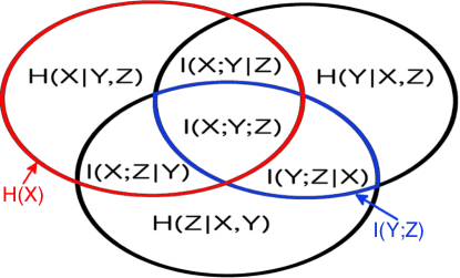
Many information-theoretic quantities of interest can be written as a sum of the ‘atoms’ of information diagrams — their smallest subunits. For example, all entropies, mutual informations, and their conditioned variants can be expressed in this way. Given constraints of this form we can calculate the maximum entropy using linear optimization.

Our methods works by constructing the information diagram with the largest entropy given the constraints, which intuitively corresponds to creating the maximally disjoint diagram. For example, conditioning on the univariate entropies alone results in the diagram being completely disjoint, i.e., the maximum entropy is the sum of the univariate entropies — a well known result. However, when conditioning on other terms, such as mutual informations, calculating the maximum entropy is no longer straightforward.

Mutual informations and entropies correspond to regions of the information diagram and can be written as the sum of the atoms in their region. In general, a system of $N$ variables, $\{X\}_{N}$, will have $2^{N}-1$ atoms corresponding to all possible possible combinations of the variables, excluding the empty set. To illustrate this, for the three variable case shown in Fig. 1 we can see the decompositions

$$I(Y;Z) = I(Y;Z|X)+I(X;Y;Z)$$ (1)

$$H(X) = H(X|Y,Z)+I(X;Y|Z)$$ (2)

$$+I(X;Z|Y)+I(X;Y;Z).$$

Any set of information-theoretic quantities can be used as constraints with our method — as long as they can be written as a linear function of the atoms of the information diagram and they bound the total entropy. This includes all $k$-variate conditional entropies and $k$-variate conditional mutual informations. The $k$-variate entropy of a set of variables $\{X\}_{k}$ conditioned on a set of variables $\{X\}_{n}$ will be the sum of the atoms in the set $\{X\}_{k}$ excluding those also in $\{X\}_{n}$, e.g., $H(X,Y|Z)=H(X|Y,Z)+H(Y|X,Z)+I(X;Y|Z)$, Fig. 1. Similarly, the $k$-variate mutual information between a set of variables $\{X\}_{k}$ conditioned on a set of variables $\{X\}_{n}$ will be the sum of the atoms that are in the intersection of all $k$ variables, but not in any atoms corresponding to $\{X\}_{n}$. If these are all the variables in the diagram this will be a single atom e.g., $I(X;Y|Z)$ in Fig. 1. We illustrate this further in Sec. IV.3 where we condition on $n$-variate entropies.

In addition to any constraints one chooses, for discrete variables, the information diagram must satisfy all the Shannon inequalities to be valid, i.e. for there to exist a probability distribution with those information-theoretic quantities. All Shannon inequalities can be constructed from elemental inequalities of the following two forms:

$$H(X_{i}|\{X\}_{N}-X_{i})\geq 0$$ (3)

and

$$I(X_{i},X_{j}|\{X\}_{K})\geq 0,$$ (4)

where $i\neq j$, and $\{X\}_{K}\subseteq\{X\}_{N}-\{X_{i},X_{j}\}$. For continuous random variables entropies can be negative, so inequalities of the form Eq. (3) are not applicable, though those of the form Eq. (4) still are. This is a minimal set of inequalities as no inequality is implied by a combination of the others. Each of these inequalities can also be written as the sum of atoms in their region. This is trivial for inequalities like Eq. (3) since all $H(X_{i}|\{X\}_{N}-X_{i})$ are themselves atoms. There will also be ${N\choose 2}$ inequalities like Eq. (4) that are atoms of the diagram. For four variables a nontrivial decomposition into atoms of an Eq. (4) inequality is

$$I(X_{1};X_{2}|X_{3})=I(X_{1};X_{2}|X_{3},X_{4})+I(X_{1};X_{2};X_{4}|X_{3})\geq 0.$$ (5)

There also exists so called non-Shannon inequalities for $N\geq 4$, which are not deducible from the Shannon inequalities Yeung2008information . While it is possible, in principle, to include these in our maximization they have not yet been fully enumerated. Therefore, we restrict the set of inequalities we use to the Shannon inequalities. As the diagram may violate a non-Shannon equality, there may be no probability distribution that satisfies it. However, the diagram would still represent an upper bound on the possible entropy.

For a large class of diagrams we do know our bound is achievable. We prove in Sec. III.1 that whenever all the atoms of the diagram are non-negative it is possible to construct a set of variables that satisfy it. It is easy to see from this proof that there will in fact be an infinite number of distributions satisfying the diagram in these cases. There will of course also be many diagrams with negative regions that are also satisfiable, but our constructive proof can not verify this.

We have now shown that the task of finding the maximum entropy, conditioned on the information-theoretic quantities discussed here, as well as the elemental Shannon inequalities, can be solved using linear optimization. Each constraint will take the form of a linear equality or inequality, as in Eq. (1) and (5), and we maximize the N-variate entropy by maximizing the sum over all $A$ atoms of the information diagram.

Our method is free of distributional assumptions, finding the maximum entropy possible for variables of any cardinality given only information-theoretic constraints. This can result in the maximum entropy diagram being unconstructable for low cardinality variables, even though it is achievable for higher cardinality ones. However this does not seem to be a large issue in practice, as can be seen in our results in Martin2015::PRL .

Given information-theoretic constraints of the type we have been discussing, it is just as easy to use linear optimization to find the minimum possible entropy as it is to find the maximum. The minimum entropy diagram is much more likely to have negative regions though, so our constructive proof of existence is not likely to hold in these cases. Analogous to the maximum entropy diagram, the minimum diagram will still represent a lower bound on the possible entropy. We focus on the maximum case because of its use in statistical physics, and more generally in statistical inference.

III Proofs

III.1 If an information diagram has only non-negative regions it can always be constructed

Given an information diagram for a set of $N$ variables, $\{X\}_{N}$, with atoms $\{A\}$, and all $A_{j}=a_{j}\geq 0$, we can always construct a probability distribution of $N$ variables that would have this diagram. We introduce a set of variables $\{Y\}$ which we define to be independent and have entropies $H(Y_{j})=a_{j}$; every region $A_{j}=a_{j}$ is associated with an independent random variable with entropy $a_{j}$. Each variable $X_{i}$ is now defined to be the set of $Y_{j}$ that have regions which lie in $H(X_{i})$.

The set of variables, $\{X\}_{N}$, will satisfy all the information regions of the diagram. We will prove this by showing that $\{X\}_{N}$ will reproduce all $H(\{X\}_{n})$, where $\{X\}_{n}$ is an $n$-variate subset of $\{X\}_{N}$. All the regions of the information diagram can be calculated from the set of $H(\{X\}_{n})$, so if $\{X\}_{N}$ reproduces this set it will reproduce the entire diagram.

The set $\{X\}_{n}$ will be the set of all $Y_{j}$ with a region associated with any of the $n$ variables in $\{X\}_{n}$. Of course some $Y_{j}$ will be included more than once, but this will not affect the entropy since $H(Y_{j},Y_{j},\{Y\}_{l})=H(Y_{j},\{Y\}_{l})$. The entropy $H(\{X\}_{n})$ would then be the sum of all the associated entropies $H(Y_{j})$, since all $Y_{j}$ are independent by definition. The sum of the entropies of $H(Y_{j})=a_{j}$ is the same as the sum of all the regions in the information diagram associated with $H(\{X\}_{n})$, and hence $\{X\}_{n}$ will satisfy all such entropies.

III.2 Analytical Maximum for $N=3$

When conditioning on bivariate mutual informations and univariate entropies we have an analytical solution for the maximum entropy when $N=3$. For three variables we can write the joint entropy as

$$H=\sum_{i}H(X_{i})-\sum_{i>j}I(X_{i};X_{j})+I(X_{1};X_{2};X_{3}).$$ (6)

We can see why Eq. (6) is true by imagining the information diagram, and realizing the total entropy must be the sum of all its elements. By adding all the univariate entropies all the conditional entropies in the information diagram are added once, but all the regions of overlap are added multiple times. These multiple counts are then removed when we remove all the mutual informations, but now we remove regions where more then 2 variables overlap too many times. For three variables we then need to add back the triplet region once. It was added three times by the entropies and removed three times by the mutual informations.

Since we are conditioning on the univariate entropies and mutual informations, the only free parameter is

$$I(X_{1};X_{2};X_{3})=I(X_{1};X_{2})-I(X_{1};X_{2}|X_{3}).$$ (7)

This means that the maximum of Eq. (6) will occur when Eq. (7) is maximal. Both $I(X_{1};X_{2})$ and $I(X_{1};X_{2}|X_{3})$ must be positive, so Eq. (7) can be no greater than the minimum mutual information between $X_{1}$, $X_{2}$, and $X_{3}$.

We now show that we can always construct this diagram when the variables are discrete since it will only have non-negative regions. Without loss of generality we can define the minimal mutual information to be $I(X_{1};X_{2})$. This results in the information diagram in Fig. 2. By inspection we can see that this diagram satisfies the constraints on the univariate entropies and mutual informations. Since $I(X_{1};X_{2})$ is the minimal mutual information, and all the mutual informations are non-negative, all the regions where multiple variables overlap in the diagram are non-negative. Now we must show that all the conditional entropies in the diagram are non-negative. The mutual information between two discrete variables can not be greater than their univariate entropies, therefore $H(X_{1}|X_{2},X_{3})\geq 0$ and $H(X_{2}|X_{1},X_{3})\geq 0$.

Figure 2: The maximum entropy diagram for three variables if the minimum mutual information between the variables is $I(X_{1};X_{2})$.

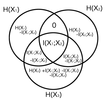
The final part now is to prove that $H(X_{3}|X_{1},X_{2})\geq 0$, which we show is true provided that the constraints are satisfiable. We now look solely at the regions inside $H(X_{3})$, and look at the affect of adding $\epsilon$ to the $I(X_{1};X_{2};X_{3})$ region. To conserve the univariate entropy and mutual informations associated with $X_{3}$, we must make the following changes

$$I(X_{1};X_{3}|X_{2})\rightarrow I(X_{1};X_{3}|X_{2})-\epsilon$$ (8)

$$I(X_{2};X_{3}|X_{1})\rightarrow I(X_{2};X_{3}|X_{1})-\epsilon$$ (9)

$$H(X_{3}|X_{1},X_{2})\rightarrow H(X_{3}|X_{1},X_{2})+\epsilon.$$ (10)

We see from this that changing one region in $H(X_{3})$ necessitates changing all the regions in $H(X_{3})$. We also see that changing $I(X_{1};X_{2};X_{3})$ changes $H(X_{3}|X_{1},X_{2})$ by the same amount. This means that the largest $H(X_{3}|X_{1},X_{2})$ can be is when $I(X_{1};X_{2};X_{3})$ is also maximal – as in our maximal construction, Fig. 2. Therefore if our constructed case resulted in $H(X_{3}|X_{1},X_{2})<0$ the constraints are unsatisfiable since this is the largest that $H(X_{3}|X_{1},X_{2})$ can be made.

Figure 2 shows that the maximum entropy, conditioned on bivariate mutual informations and univariate entropies, corresponds to the pair of variables with the smallest mutual information being conditionally independent. This is notable, as it is essentially what is done in Margolin2006::BMCbioinfo , where they attempt to infer interactions between genes; for every triplet of genes they consider the pair with the smallest mutual information to be independent. While they justify this using the data processing inequality Cover2006 , our proof here lends this procedure further credibility.

III.3 Proof that conditioning on the first two moments is equivalent to conditioning on bivariate distributions for binary variables

Maximizing the joint entropy of a set of binary variables, conditioned on their first two moments, is the same as conditioning on the joint probability distributions. The univariate distributions can be reconstructed from the first moments

$$E[X] = x_{0}p(x_{0})+x_{1}(1-p(x_{0}))$$ (11)

$$p(x_{0}) = \frac{E[X]-x_{1}}{x_{0}-x_{1}}.$$ (12)

This information plus the covariances exactly specify the bivariate distributions. For the bivariate distributions we have

$$p(x_{0},y_{0})+p(x_{1},y_{0})=p(y_{0})$$ (13)

$$p(x_{0}|y_{0})p(y_{0})+p(x_{1}|y_{0})p(y_{0})=p(y_{0})$$ (14)

$$p(x_{0}|y_{0})+p(x_{1}|y_{0})=1$$ (15)

$$p(x_{0}|y_{0})+\frac{p(x_{1})-p(x_{1}|y_{1})p(y_{1})}{p(y_{0})}=1$$ (16)

$$p(x_{0}|y_{1})+p(x_{1}|y_{1})=1$$ (17)

Therefore, for the 2-variable conditional probabilities there is only one degree of freedom when the marginal probabilities are known, which is equivalent to the covariance

$$C[X,Y] = x_{0}y_{0}p(x_{0},y_{0})+x_{0}y_{1}p(x_{0},y_{1})+x_{1}y_{0}p(x_{1},y_{0})$$

$$+x_{1}y_{1}p(x_{1},y_{1})$$

$$p(x_{0}|y_{0}) = [C[X,Y]-x_{0}y_{1}p(x_{0})-x_{1}y_{0}p(y_{0})$$

$$+x_{1}y_{1}(p(y_{0})-p(x_{1}))]$$

$$\times\left[p(y_{0})(x_{0}y_{0}-x_{1}y_{0}-x_{0}y_{1}+x_{1}y_{1})\right]^{-1}.$$

Therefore, maximizing the entropy conditioned on the first two moments of a set of binary variables is equivalent to maximizing the entropy conditioned on their bivariate probability distributions.

IV Applications

IV.1 Undersampled Regime

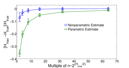
Possibly one of the most exciting applications of our method is in the undersampled regime. It is possible to estimate the entropy of a set of discrete variables with $n\sim 2^{H/2}$ samples (where $H$ is measured in bits) Nemenman2011::Ent . This means it is possible to make maximum entropy estimates even when the marginal probability distributions have not been sufficiently sampled, as needed to calculate the connected informations in Schneidman2003::PRL .

As an example, consider an Ising type model with probability distribution,

$$P(\mathbf{X})=\frac{1}{Z}\exp\left(\sum_{i=1}^{N}h_{i}x_{i}+\sum_{i>j}J_{i,j}x_{i}x_{j}\right),$$ (18)

where $Z$ is a normalization constant. These distributions often arises in the context of establishing the importance of pairwise interactions, because they describe the maximum entropy distribution consistent with the first two moments of a set of variables Martin2015::PRL ; Timme2014 . Therefore, we would expect the difference between the entropy of the true distribution and the maximum entropy conditioned on the bivariate distributions to be zero.

At small sample sizes however, the maximum entropy is severely underestimated when conditioning on naively estimated bivariate distributions. On the other hand, a much more accurate estimate of the maximum entropy is obtained when estimating the univariate and bivariate entropies using the estimator in Nemenman2011::Ent , and using these as constraints in our nonparametric method. This is shown in Fig. 3.

Figure 3: (Color online) The fractional difference between the maximum entropy estimate and the true entropy using our nonparametric maximum calculated from the univariate and bivariate entropies, as well as estimating the maximum parametrically from the estimated bivariate probability distributions. One hundred distributions of three variables of the form Eq. (18) were generated with the parameters $h_{i}$ and $J_{i,j}$ drawn from normal distributions with zero mean and standard deviation $0.1$, with each variable having a cardinality of 5. The minimum number of samples needed, $n\sim 2^{H/2}$, ranged from 4 to 12. The error bars are given by the $25\%$ and $75\%$ quantiles.

IV.2 Computation Time

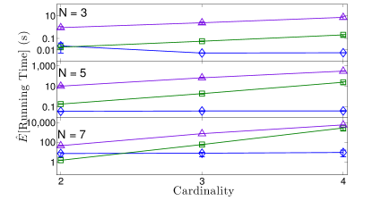
To illustrate the potential computational speedups possible using our methods, we consider Ising type distributions, Eq. (18), again. Specifically, we investigate the dependence on different numbers of random variables, $N$, and variable cardinality. In each case the parameters $h_{i}$ and $J_{i,j}$ are drawn from a normal distribution with mean zero and variance $0.1$.

Figure 4 compares the runtime of our algorithm with that using iterative proportional fitting Darroch1972::AnMatStat , where we show both conditioning on the bivariate distributions and conditioning on the first two moments of the distributions. Since our method only uses information-theoretic quantities as inputs it is not affected by the cardinality of the variables, i.e., if the variables have a cardinality of two or 100 it will have no bearing on how long our method takes to run, as long as the information-theoretic quantities conditioned on are the same. As the other methods do depend on the cardinality of the variables we expect that at ‘some’ cardinality our method will certainly outperform them. In fact, as Fig. 4 shows, only when the variables have a cardinality of two are the runtimes comparable, with our method running orders of magnitude faster at all measured higher cardinalities.

Figure 4: (Color online) The expected running time for different methods at different variable cardinalities, and number of variables, $N$. The three methods are: our linear optimization method conditioned on mutual informations and univariate entropies (blue diamonds); iterative fitting conditioned on the bivariate distributions (green squares); iterative fitting conditioned on the first two moments (purple triangles). For each cardinality and $N$, the distributions and error calculations are the same as for Fig. 3.

IV.3 Estimating connected informations

Next we show how our method can be used to nonparametrically estimate connected informations Schneidman2003::PRL , which are useful for estimating the relevance of higher-order interactions in sets of variables. However, as the number of variables and their cardinality increases, estimating these values from the probabilities directly can suffer from lack of samples do to the exponentially increasing phase space, as well as quickly become computationally intractable.

In order to estimate connected informations using our method we condition on $n$-variate entropies. This lets us answer the question of what the maximum possible $N$-variate entropy is given any set of entropies. Let $a_{\{X\}_{k}}$ be the set of all atoms that lie in the joint entropy $H(\{X\}_{k})$. The univariate entropy $H(X_{i})$ is the sum of all atoms $a_{X_{i}}$. Similarly, the bivariate entropy $H(X_{i},X_{j})$ is the sum of all atoms $a_{\{X_{i},X_{j}\}}$. This is easily generalized to the $n$-variate entropy $H(\{X\}_{n})$, which is the sum of all atoms $a_{\{X\}_{n}}$. Therefore, we can use any $n$-variate entropy as a constraint in the linear optimization problem.

The connected information of order $k$ is,

$$I_{C}^{(k)}(\{X\}_{N})=H[\widetilde{P}^{(k-1)}(\{X\}_{N})]-H[\widetilde{P}^{(k)}(\{X\}_{N})],$$ (19)

where $\widetilde{P}^{(k)}(\{X\}_{N})$ is the maximum entropy distribution consistent with all $k$-variate marginal distributions. Instead of this we propose an alternate expression

$$I_{C}^{(k)}=\widetilde{H}^{(k-1)}-\widetilde{H}^{(k)},$$ (20)

where $\widetilde{H}^{(k)}$ is the maximum entropy consistent with all the one through $k$-variate entropies.

This formulation has three advantages: 1) estimating the $k$-variate marginal distributions can be problematic do to insufficient data, whereas much better estimates of the $k$-variate entropies may be available such as Nemenman2011::Ent , as we showed in Sec. IV.1; 2) this equation is easily estimated using our maximum entropy estimation, which can offer significant computational speedups over existing techniques, as we showed in Sec. IV.2; 3) this can be estimated given just the information-theoretic quantities independent of any specific knowledge of the underlying distributions.

It is important to realize though that Eqs. (19) and (20) differ in that the latter does not constrain the cardinality of the variables and could violate the non-Shannon inequalities as discussed in Section II. Therefore, it will always be the case that $\widetilde{H}^{(k-1)}\geq H[\widetilde{P}^{(k-1)}(\{X\}_{N})]$. In the examples we have looked at before Martin2015::PRL , as well as in the illustrative example we give next, this does not seem to appreciably affect the results however.

IV.3.1 Illustrative Example

The quintessential example of an entirely 3-variate interaction is the Exclusive OR (XOR) gate when the inputs are chosen uniformly and independently, the truth table of which is given in Table 1. Any pair of variables taken alone appear to be independent, though given the state of two the state of the third is uniquely determined. This can be generalized to an $N$-variate relationship by taking $N-1$ independently generated random variables uniformly drawn from the set $\{0,1\}$, and the $N$th their sum modulo two. We can also generalize to arbitrary cardinalities, $C$, by drawing the $N-1$ variables independently and uniformly from the set $\{0,..,C-1\}$, and the $N$th is now their sum modulo $C$.

$X$	$Y$	$Z$
0	0	0
1	0	1
0	1	1
1	1	0.

Table 1: Truth table for an Exclusive OR (XOR) gate, where the inputs are $X$ and $Y$, and the output is $Z$.

We now show that in these cases our nonparametric connected information, Eq. (20), will return the same result as the parametric one, Eq. (19). Given a set of $N$ variables with cardinality $C$, and an $N$-variate interaction of the type discussed above, the joint entropy of any set of $k<N$ variables will be the sum of the univariate entropies, $H(\{X\}_{k})=\sum H(X_{i})$. This means for both Eq. (20) and 19, $I_{c}^{(k)}=0$ for $k<N$. For $k=N$, both $\widetilde{H}^{(k)}$ and $H[\widetilde{P}^{(k)}(\{X\}_{N})]$ are the true $N$-variate entropies, and $I_{c}^{(k)}=H(X_{i})$ in both cases. We can see from this that both methods will also return the same result for a system of $N$ variables that is composed of independent sets of $n$ variables with $n$-variate relationships, where $n$ is allowed to differ between sets, e.g. two XOR gates, where $N=6$ and $n=3$ for both sets.

IV.4 Resting-State Human Brain Networks

To illustrate the applicability of the described methodology in real-world data situations, we apply it to neuroimaging data, in a similar context as in the recent study by Watanabe et al Watanabe2013::NatCom . In particular, we want to assess to what extent the multivariate activity distribution is determined by purely bivariate dependence patterns. This is of relevance because the use of bivariate dependence matrices, particularly of pairwise correlations, is currently a prominent method of characterizing the brain interaction structure. If pairwise relationships are sufficient to describe the interaction structure of the brain this would tremendously simplify the task of uncovering this structure. If this were not the case, it would mean that higher-order relationships, as discussed in Sec. IV.3, would need to be analyzed. As the phase space of the problem grows exponentially as we probe ever higher-order interactions, this would result in us rapidly running out of sufficient data to sample these spaces, and measure the corresponding interactions.

The used data consist of time series of functional magnetic resonance imaging signal from 96 healthy volunteers measured using a 3T Siemens Magnetom Trio scanner in IKEM (Institute for Clinical and Experimental Medicine) in Prague, Czech Republic. Average signals from 9 regions of the well-known default mode network, and 12 regions of the fronto-parietal network were extracted using a brain atlas Shirer2011 . Standard preprocessing and data denoising was carried out using processing steps described in a previous neuroimaging study Hlinka2011Neuroimage . The data were temporally concatenated across subjects to provide a sufficient sample of $T=36480$ timepoints. Each variable was further discretized to 2 or 3 levels using equiquantal binning. Entropies were then estimated using the estimator in Nemenman2011::Ent . We tested that we could estimate the full joint entropy by estimating it for increasing sample sizes, and checking that the estimate stabilized for the largest available sample sizes. Moving to larger cardinalities was not possible due to insufficient data available to estimate the full joint entropy of the resting-state networks.

Our analysis of the default mode network resulted in $I_{m}/I_{N}=1$ and $0.90$ for the 2-level and 3-level discretizations respectively, when conditioning on the first two moments, and $0.86$ and $0.90$ when using our technique conditioned on bivariate mutual informations and univariate entropies. Similarly, for the fronto-parietal network, conditioning on the moments resulted in $I_{m}/I_{N}=1$ and $0.73$ for the 2-level and 3-level discretizations, and $0.77$ for both discretizations when using our method. In both cases we can see that conditioning on the first two moments resulted in a substantial decrease in $I_{m}/I_{N}$ as the discretization was increased, while the results using our method appear stable to the discretization. The effect of discretization on both these methods is in accord with the results for nonlinear model systems in Martin2015::PRL .

Overall, our findings are consistent with the observations reported in Watanabe2013::NatCom for the 2-level and 3-level discretization of the default mode network and the fronto-parietal network, where they conditioned on the first two moments only. For 2-level discretization, they found $I_{m}/I_{N}=0.85$ and $0.96$ for the default mode and fronto-parietal networks respectively. For the 3-level discretization, the ratio dropped to $I_{m}/I_{N}\approx 0.55$ for both networks. The variation between their specific values and ours — especially for the 3-level discretization — is likely a result of the different regions used to represent both networks in combination with statistical variations starting from different data sets to begin with. In conclusion, both their and our findings indicate that nonlinear relationships play an important role in the structure of fMRI data.

IV.5 Network inference

In the process of finding a maximum entropy estimate, the linear optimization computes all the atoms of the information diagram. This includes the conditional mutual information (CMI) between every variable pair, conditioned on every other variable. This can be interpreted as the level of direct pairwise interaction between components of a dynamical system and thus be used as a novel method for inferring structural connectivity, provided that the interactions are predominately pairwise in the first place. In the following section we show how using our entropy maximization conditioned on mutual informations and univariate entropies outperforms other techniques; in particular relevance networks as defined in butte2000mutual , which work by picking a threshold for a statistical similarity measure (in our case the mutual information), and interpreting every pair of variables that cross this threshold as directly interacting. To benchmark our method’s performance we analyze the Kuramoto model as a paradigmatic dynamical system with non-linear coupling.

IV.5.1 The model

The Kuramoto model was introduced in kuramoto1975self and consists of $N$ phase oscillators that are coupled in a particular topology. The $i$th oscillator’s frequency is given by $\theta_{i}$ and its dynamics are described by

$$\frac{\partial\theta_{i}}{\partial t}=\omega_{i}+\frac{K}{N}\sum_{j=1}^{N}\sigma_{ij}\sin(\theta_{j}-\theta_{i})+\eta_{i}(t).$$ (21)

Here $\omega_{i}$ is the natural frequency of the oscillator, and $\eta_{i}(t)$ a random noise term drawn from a Gaussian distribution with correlation function $<\eta_{i}(t),\eta_{j}(t^{\prime})>=G\delta_{ij}\delta(t-t^{\prime})$, where G determines the amplitude of the noise. $K$ represents a uniform coupling strength between interacting nodes, and $\sigma_{ij}\in\{0,1\}$ represents the adjacency matrix of the network, where $\sigma_{i,j}=1$ for connected nodes. The interactions are always taken to be bidirectional, i.e. $\sigma_{ij}=\sigma_{ji}$. In the following, we focus on the case when the adjacency matrix is an Erdös-Rènyi random graph Erdos1960 of density $p$, with a fixed number of links. The inference problem is then to reconstruct $\bm{\sigma}$ from the measured time series $\theta_{i}$.

The time series are generated using the Euler-Maruyama method with a step size $dt=2^{-6}$ and noise amplitude $G=0.05$. The data gets resampled such that only every 8th time step is used, and a transient of $T_{trans}=50$ is removed. Unless stated otherwise the network size is $N=12$, the integration time $T=50,000$, the coupling strength $K=0.5$, the number of links in the network $12$ (which corresponds to each node having an average of 2 neighbors and $p\approx 0.18$).

The data is discretized using equiquantal binning into $n=3$ states. Numerical tests (using $n=5$ and $n=7$) have indicated that larger cardinalities can improve the performance, given that the used time series is long enough. Otherwise sampling issues may arise (i.e. empty or almost empty bins) and degrade the quality of the entropy estimation. The intrinsic frequencies are drawn from a uniform distribution on the interval $[\Omega,3\Omega]$ with $\Omega=20\cdot\frac{p}{N}$. For higher values of $p$ synchronization effects would be expected at lower coupling strengths. To counteract this, the frequency scale increases with $p$. The distribution is shifted away from zero to sample through the phase space more quickly, i.e. avoid oscillators that stay in just one bin throughout the system’s time evolution.

IV.5.2 The method

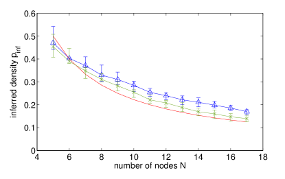
The presented maximum entropy estimator calculates CMI between each pair of oscillators conditioned on every other oscillator from supplied constraints on the estimated mutual information and univariate entropies. A link is inferred if the CMI between the two oscillators is nonzero. However, we find, for a given system size, the average inferred density doesn’t depend much on the actual density of the network. Figure 5 shows the maximum density for varying network sizes. If a network of higher density is analyzed, the method can still be expected to infer existing links, however it will fail to identify a significant number of true links. This is a result of the method having at least one zero conditional information for all subsets of variables greater than two, so for example this method will not infer any triangles, see Sec. III.2. If in contrast a network is analyzed that is sparser than the average density inferred by the method, our findings necessitates the use of a threshold to reduce the detection of spurious links.

To speed up the optimization we use a strictly stronger set of inequalities here, where it is assumed that every atom is non-negative. This provides a lower bound for the maximum entropy. If interactions are truly described by bivariate interactions only, then negative atoms are expected to be negligible, as they would indicate higher-order interactions. This approximation should only be employed if pairwise interactions have already been established as a good model, which we tested for the Kuramoto model in Martin2015::PRL . Numerical comparisons at smaller system sizes have indicated that this is indeed a viable approximation. To that end 100 realization with a length of $T=10,000$ were evaluated at a system size of $N=9$ using both the exact constraints and the approximate ones. The biggest relative error of the approximate maximum entropy estimate was $0.087\%$.

Figure 5: (Color online) Average inferred link densities $p_{inf}$ as a function of network size, if our maximum entropy method is applied using unthresholded estimated mutual informations. The actual network densities are $p=0.1$ (blue triangles), and $p=1$ (green crosses). The red curve is the density of a network in which every node interacts with two neighbors on average, and given for comparison. The inferred density is calculated as the number of inferred links over the number of possible links, ${N\choose 2}$. Each curve is generated from 100 realizations of natural frequencies and adjacency matrices with given density $p$. The error bars are given by the $25\%$ and $75\%$ quantiles.

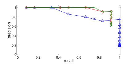
For global thresholding there are two obvious options: either threshold the mutual informations and then apply our maximization procedure, or apply our maximum entropy method first and then threshold the CMI matrix. Our assessment of the method’s performance is based on the precision (ratio of correctly inferred links to all the inferred links) and the recall (ratio of correctly inferred links over existing links) (see for example rijsbergen1979information ). As shown in Fig. 6, using these valuation metrics neither approach seems to be superior over the other. Both ways generally improve the performance of merely thresholding the mutual information without using any maximum entropy method at all.

Figure 6: (Color online) Representative precision/recall curves: Thresholding of MI matrix alone, and not using any maximum entropy method (blue triangles); thresholding of CMI matrix obtained using our maximum entropy method on the (unthresholded) mutual informations (green crosses); thresholding of mutual informations, and then using the maximum entropy method (red diamonds).

To make this observation more quantitative, it is useful to have a single real number valuation metric to compare performances. We have chosen the $F_{1}$-score rijsbergen1979information , defined as $F_{1}=2\cdot\frac{precision\cdot recall}{precision+recall}$, because it treats precision and recall symmetrically and it is not clear that either measure should be preferred in a general context. From Fig. 7 it is apparent that the best performance is achieved at $K\approx 0.5$. Considering the coupling is given as $\frac{K}{N}=\frac{0.5}{12}\approx 0.042$ which is of the same order of magnitude as the noise $G=0.05$, this indicates that our method performs particularly well in the weak coupling regime where no oscillators are synchronized.

Figure 7: (Color online) For different thresholding methods the global threshold has been picked that leads to the highest $F_{1}$-score (left). The precision corresponding to that threshold is also plotted for comparison (right). The symbols are the same as in Fig. 6. The process has been applied to an ensemble of 100 realizations and the averages are shown. Error bars are given by the $25\%$ and $75\%$ quantiles.

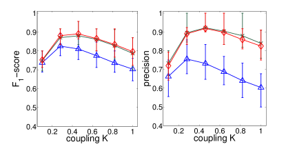
Figure 7 also shows that a generally higher precision and $F_{1}$-score can be achieved using our method as an additional step after the mutual information thresholding, only partially compromising the recall. The problem of finding a suitable global threshold that actually achieves that performance remains open. In the following section we outline a surrogate based method of finding a non-global threshold that displays a performance comparable to the global thresholding discussed above.

IV.5.3 Finding significance thresholds

A problem for the method’s performance on the Kuramoto model is posed by the fact that two disconnected nodes can have a high estimated mutual information in a finite time series, if their effective frequencies are close to each other. To account for this we generate surrogates that preserve these effective frequencies as well as the oscillator’s autocorrelations. First the effective frequencies are removed from the time series, subtracting from each oscillator the linear function that interpolates between the initial and final value of their unwrapped phase. That way each oscillator’s time series begins and ends at the same value. In the next step, the Iterative Amplitude Adapted Fourier Transform Algorithm (IAAFT) Schreiber1996::PRL is applied to the trend-removed time series. As a last step, the trends are added back in and for each oscillator a random number uniformly drawn from $0$ to $2\pi$ is added to every value of the time series. This corresponds to randomizing the initial conditions. The mutual informations between the so obtained time series are estimated in the same way as before. This provides an estimate for the mutual information for each pair of oscillators that is not due to their coupling.

To obtain a (local) threshold, a statistical significance level has to be chosen. Since higher significance levels require more surrogate series, the problem can become computationally very expensive. In Margolin2006::BMCbioinfo they suggest that good performance can be expected in the regime of $q\approx 98.5\%$, because there are $12\choose{2}$ $=66$ possible links in our system and $\frac{1}{66}\approx 1.5\%$. The rational behind this is pick $q$ so that we expect to keep on average one false link with this threshold.

Figure 8: (Color online) A single typical realization of a precision/recall curve for only thresholding the mutual information (blue triangles) and the maximum entropy method being applied to thresholded mutual informations (red diamonds), similar to Fig. 6. The blue square filled green shows the performance of applying local thresholds to the MI matrix and the red circle filled green the performance of applying the method to the locally thresholded mutual informations. The thresholds are determined by the surrogate method discussed in the main text using the $q=98.5$ percentile. 700 surrogates were generated.

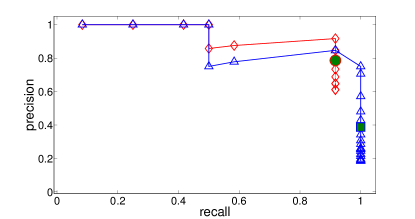
As Fig. 8 indicates, the surrogate-based local thresholding method achieves good performance after our maximum entropy method is applied. This claim is substantiated by statistics as shown in Table 2, clearly establishing the benefit of our maximum entropy method.

	precision	recall	$F_{1}$-score
mutual informations only	0.369	0.997	0.534
with maximum entropy method	0.772	0.834	0.789

Table 2: Performance of local thresholding averaged over 100 realizations with $T=10,000$ and $q=90\%$ using 100 surrogates each. The CMI achieved a higher $F_{1}$-score in all but 3 cases. The average difference in performance was $\Delta F_{1}=0.255(+0.079,-0.045)$ with $25\%$ and $75\%$ quantiles given.

V Discussion & Conclusions

In this paper we extended the method we introduced in Martin2015::PRL to compute the maximum entropy conditioned on a wide range of information-theoretic quantities — beyond the bivariate mutual informations and univariate entropies — using linear optimization. We have also shown how to implement our method with continuous variables, no longer limiting it to discrete ones, making our technique applicable to a much broader range of problems. While there are pathological linear optimization problems whose running time will scale exponentially with the number of variables, $N$, there will always be a slightly perturbed problem such that our method will scale polynomially Vershynin2009::SJC .

Our method is nonparametric in that it does not generate a corresponding probability distribution. This may result in a diagram for which no probability distribution can be constructed (since it may violate a non-Shannon inequality). However, we proved in Sec. III.1 that in the common case where the maximum diagram has only non-negative regions it will indeed be satisfiable.

Since our methods do not require the direct estimate of any probability distribution, we can apply them in the undersampled regime. We demonstrated in Sec. IV.1 that in this regime our method offers a much more accurate estimate of the maximum entropy. Additionally, in Sec. IV.2 we demonstrated that our method offers computational speedups over competing techniques when the variables have cardinality greater than 2. This makes our techniques perfectly positioned to analyze systems of larger cardinality variables where the size of the phase space can make both computation time and accurate sampling prohibitive.

Motivated by our new ability to easily compute the maximum entropy given information-theoretic constraints, we introduced a nonparametric formulation of connected informations, Sec. IV.3. This can be computed directly using our linearly optimized maximum entropy, and hence has its computational and sampling advantages. For paradigmatic examples of higher-order relationships — which connected informations attempt to detect — we demonstrated that our nonparametric method will give the same result as the standard one, Sec. IV.3.1.

We have also expanded on our work in Martin2015::PRL , where we have now analyzed two resting-state human brain networks. It is highly desirable to know if these networks can be accurately described with pairwise measurements, as it would tremendously simplify their analysis, and is common practice. Previous results indicated that this is the case, but only when the signal is binarized Watanabe2013::NatCom . In both networks analyzed we have shown that conditioning on the first two moments of the distributions exhibits a marked sensitivity to the number of states the system is discretized to, Sec. IV.4. On the other hand our method appears to be robust to the specific discretization, as was also seen in Martin2015::PRL for the case of the Kuramoto model. This indicates that pairwise measurements can still capture the vast majority of the complexity of these networks, but only when nonlinear relationships are taken into account.

Finally, we used our entropy maximization method to infer conditional mutual informations, and hence to infer the structural connectivity of a network, Sec. IV.5. We showed that our maximum entropy estimation can be used to improve on the performance of naively thresholding the mutual informations to infer networks of a dynamical system. For the Kuramoto model it was also evident that our method performs particularly well in the weak coupling regime, where other methods do struggle. For example, the main method proposed in Ref. Tirabassi2015::SR achieved its best results for the Kuramoto model in the strong coupling regime.

We also managed to demonstrate that our particular thresholding method achieves high precision, while also retaining higher recall than, for example, in Ref. Margolin2006::BMCbioinfo . There they used a method similar in spirit to ours, where they estimated the network based on the thresholded mutual information between all pairs of variables, as well as set the weakest mutual information between every triplet of variables to zero. While they justified this with the data processing inequality, we showed in Sec. III.2 that this also can justified as a result of maximum entropy estimation, giving further credence to their method. It must be noted however, that bigger system sizes and higher link densities were considered in Ref. Margolin2006::BMCbioinfo than can be treated with our presented method.

In conclusion, we have shown that our entropy maximization performs well in the undersampled regime, and for high cardinality variables. This helps resolve two outstanding problems with maximum entropy estimation, as noted in Yeh2010::Ent . We have also shown that this method can be applied to real world problems facing researchers, using fMRI data and network inference as examples. While we have given a few obvious applications for our method, given its broad nature it is our belief that many researchers will find uses for it that we have yet to anticipate.

This project was financially supported by NSERC (EM and JD) and by the Czech Science Foundation project GA13-23940S and the Czech Health Research Council project NV15-29835A (JH). AM was financially supported by the DAAD. All authors would like to thank the MPIPKS for its hospitality and hosting the international seminar program “Causality, Information Transfer and Dynamical Networks”, which stimulated some of the involved research. We also would like to thank P. Grassberger for many helpful discussions.

References

- (1) Edwin T Jaynes. Information theory and statistical mechanics. Phys. Rev., 106(4):620, 1957.
- (2) Elad Schneidman, Michael J Berry, Ronen Segev, and William Bialek. Weak pairwise correlations imply strongly correlated network states in a neural population. Nature, 440(7087):1007–1012, 2006.
- (3) Timothy R Lezon, Jayanth R Banavar, Marek Cieplak, Amos Maritan, and Nina V Fedoroff. Using the principle of entropy maximization to infer genetic interaction networks from gene expression patterns. Proc. Natl. Acad. Sci., 103(50):19033–19038, 2006.
- (4) K. Wood, S. Nishida, E. D. Sontag, and P. Cluzel. Mechanism-independent method for predicting response to multidrug combinations in bacteria. Proc. Natl. Acad. Sci., 109(30):12254–12259, 2012.
- (5) Elad Schneidman, Susanne Still, Michael J Berry, William Bialek, et al. Network information and connected correlations. Phys. Rev. Lett., 91(23):238701, 2003.
- (6) G. J. Stephens and W. Bialek. Statistical mechanics of letters in words. Phys. Rev. E, 81:066119, Jun 2010.
- (7) T. M. Cover and J. A. Thomas. Elements of information theory. John Wiley & Sons, 2006.
- (8) Ilya Nemenman. Coincidences and estimation of entropies of random variables with large cardinalities. Entropy, 13(12):2013–2023, 2011.
- (9) E. A. Martin, J. Hlinka, and J. Davidsen. Pairwise network information and nonlinear correlations. Submitted to Phys. Rev. Lett.
- (10) F. C. Yeh, A. Tang, J. P. Hobbs, P. Hottowy, W. Dabrowski, A. Sher, A. Litke, and J. M. Beggs. Maximum entropy approaches to living neural networks. Entropy, 12(1):89–106, 2010.
- (11) T. Watanabe, S. Hirose, H. Wada, Y. Imai, T. Machida, I. Shirouzu, S. Konishi, Y. Miyashita, and N. Masuda. A pairwise maximum entropy model accurately describes resting-state human brain networks. Nat. Commun., 4:1370, 2013.
- (12) M. Timme and J. Casadiego. Revealing networks from dynamics: an introduction. J. Phys. A Math. Theor., 47(34):343001, 2014.
- (13) V. M. Eguiluz, D. R. Chialvo, G. A Cecchi, M. Baliki, and A. V. Apkarian. Scale-free brain functional networks. Phys. Rev. Lett., 94(1):018102, 2005.
- (14) A. A. Margolin, I. Nemenman, K. Basso, C. Wiggins, G. Stolovitzky, R. D Favera, and A. Califano. Aracne: an algorithm for the reconstruction of gene regulatory networks in a mammalian cellular context. BMC Bioinformatics, 7(Suppl 1):S7, 2006.
- (15) J. Runge, V. Petoukhov, J. F. Donges, J. Hlinka, N. Jajcay, M. Vejmelka, D. Hartman, N. Marwan, M. Paluš, and J. Kurths. Identifying causal gateways and mediators in complex spatio-temporal systems. Nat. Commun., 6, 2015.
- (16) G. Tirabassi, R. Sevilla-Escoboza, J. M Buldú, and C. Masoller. Inferring the connectivity of coupled oscillators from time-series statistical similarity analysis. Sci. Rep., 5, 2015.
- (17) S. Frenzel and B. Pompe. Partial mutual information for coupling analysis of multivariate time series. Phys. Rev. Lett., 99(20):204101, 2007.
- (18) J. Runge and J. Davidsen. Continuous random variables and time graphs. In Preperation.
- (19) Raymond W Yeung. Information theory and network coding. Springer, 2008.
- (20) J. N. Darroch and D. Ratcliff. Generalized iterative scaling for log-linear models. Ann. Math. Stat., 43(5):1470–1480, 1972.
- (21) W. R. Shirer, S. Ryali, E. Rykhlevskaia, V. Menon, and M. D. Greicius. Decoding subject-driven cognitive states with whole-brain connectivity patterns. Cereb. Cortex, 2011.
- (22) J. Hlinka, Milan Paluš, M. Vejmelka, D. Mantini, and M. Corbetta. Functional connectivity in resting-state fMRI: Is linear correlation sufficient? NeuroImage, 54:2218–2225, 2011.
- (23) A. J. Butte and I. S. Kohane. Mutual information relevance networks: functional genomic clustering using pairwise entropy measurements. In Pac. Symp. Biocomput., volume 5, pages 418–429. World Scientific, 2000.
- (24) Y. Kuramoto. Self-entrainment of a population of coupled non-linear oscillators. In International symposium on mathematical problems in theoretical physics, pages 420–422. Springer, 1975.
- (25) P. Erdös and A. Rényi. On the evolution of random graphs. Publ. Math. Inst. Hung. Acad. Sci, 5:17–61, 1960.
- (26) C. J. Rijsbergen. Information retrieval. online book http://www.dcs.gla.ac.uk/Keith/Chapter.7/Ch.7.html. Butterworth-Heinemann, 1979.
- (27) T. Schreiber and A. Schmitz. Improved surrogate data for nonlinearity tests. Phys. Rev. Lett., 77(4):635, 1996.
- (28) R. Vershynin. Beyond hirsch conjecture: Walks on random polytopes and smoothed complexity of the simplex method. SIAM J. Comput., 39(2):646–678, 2009.