Polymers with nearest- and next nearest-neighbor interactions on the Husimi lattice

Tiago J. Oliveira111On leave at Ames Laboratory - USDOE and Department of Physics & Astronomy, Iowa State University, Ames, Iowa 50011, United States tiago@ufv.br Departamento de Física, Universidade Federal de Viçosa, 36570-900, Viçosa, MG, Brazil
Abstract

The exact grand-canonical solution of a generalized interacting self-avoid walk (ISAW) model, placed on a Husimi lattice built with squares, is presented. In this model, beyond the traditional interaction ω1=eϵ1/kBTsubscript𝜔1superscript𝑒subscriptitalic-ϵ1subscript𝑘𝐵𝑇\omega_{1}=e^{\epsilon_{1}/k_{B}T} between (nonconsecutive) monomers on nearest-neighbor (NN) sites, an additional energy ϵ2subscriptitalic-ϵ2\epsilon_{2} is associated to next-NN (NNN) monomers. Three definitions of NNN sites/interactions are considered, where each monomer can have, effectively, at most 2, 4 or 6 NNN monomers on the Husimi lattice. The phase diagrams found in all cases have (qualitatively) the same thermodynamic properties: a non-polymerized (NP) and a polymerized (P) phase separated by a critical and a coexistence surface that meet at a tricritical (θ𝜃\theta-) line. This θ𝜃\theta-line is found even when one of the interactions is repulsive, existing for ω1subscript𝜔1\omega_{1} in the range [0,)0[0,\infty), i. e., for ϵ1/kBTsubscriptitalic-ϵ1subscript𝑘𝐵𝑇\epsilon_{1}/k_{B}T in the range [,)[-\infty,\infty). Counterintuitively, a θ𝜃\theta-point exists even for an infinite repulsion between NN monomers (ω1=0subscript𝜔10\omega_{1}=0), being associated to a coil-“soft globule” transition. In the limit of an infinite repulsive force between NNN monomers, however, the coil-globule transition disappears and only a NP-P continuous transition is observed. This particular case, with ω2=0subscript𝜔20\omega_{2}=0, is also solved exactly on the square lattice, using a transfer matrix calculation, where a discontinuous NP-P transition is found. For attractive and repulsive forces between NN and NNN monomers, respectively, the model becomes quite similar to the semiflexible-ISAW one, whose crystalline phase is not observed here, as a consequence of the frustration due to competing NN and NNN forces. The mapping of the phase diagrams in canonical ones is discussed and compared with recent results from Monte Carlo simulations.

I Introduction

A polymer in solution, usually, may exist in three different conformations depending on temperature T𝑇T or solvent quality: i) extended: coil-like chains (high T𝑇T and/or good solvents); ii) collapsed: the chains have globule-like shapes (low T𝑇T and/or poor solvents); and iii) θ𝜃\theta: this point marks the (continuous/tricritical DeGennes1 ; DeGennes2 ) transition between the coil and globule phases (occurring at Tθsubscript𝑇𝜃T_{\theta} and in a “θ𝜃\theta-solvent”) Flory1 ; Flory2 . The differences among these phases can be characterized, for example, through the metric exponent ν𝜈\nu - from the scaling of the gyration radio Rgsubscript𝑅𝑔R_{g} with the number N𝑁N of monomers, RgNνsimilar-tosubscript𝑅𝑔superscript𝑁𝜈R_{g}\sim N^{\nu} -, being νcoil>νθ>νglobulesubscript𝜈𝑐𝑜𝑖𝑙subscript𝜈𝜃subscript𝜈𝑔𝑙𝑜𝑏𝑢𝑙𝑒\nu_{coil}>\nu_{\theta}>\nu_{globule}.

For linear polymers, the coil phase can be modeled by self-avoiding walks (SAWs), where the excluded volume is the only interaction present (athermal system). Generalizing this model, by including self-attraction in the chain, the globule phase as well as a coil-globule transition arise. When the polymer is placed on a lattice, the standard interacting SAW (ISAW) model consists in assigning an energy ϵitalic-ϵ\epsilon (yielding an attractive force) between monomers on nearest-neighbor (NN) sites nonconsecutive in the walk Carlo ; Flory2 ; DeGennes2 . Coil and globule phases, separated by a tricritical (θ𝜃\theta)-point, are indeed observed in this model. In two-dimensions, the exponents νcoil=3/4subscript𝜈𝑐𝑜𝑖𝑙34\nu_{coil}=3/4, νθ=4/7subscript𝜈𝜃47\nu_{\theta}=4/7 and νglobule=1/2subscript𝜈𝑔𝑙𝑜𝑏𝑢𝑙𝑒12\nu_{globule}=1/2 are exactly known Flory1 ; DupSaleur ; Carlo . The more general case of semiflexible polymers has been modeled by introducing a bending energy ϵbsubscriptitalic-ϵ𝑏\epsilon_{b} in the ISAW model (see for instance Refs. jurgenSF1 ; Lise ; pretti ; Zhou2 ). In this semiflexible-ISAW (sISAW) model, a stable crystalline (solid-like) phase also exists in the system (for low T𝑇T and large ϵbsubscriptitalic-ϵ𝑏\epsilon_{b}), in addition to the coil and globule ones.

Lee et al. Lee1 ; Lee2 have proposed another interesting generalization of the ISAW model by associating different energies ϵ1subscriptitalic-ϵ1\epsilon_{1} and ϵ2subscriptitalic-ϵ2\epsilon_{2} to monomers on NN and next-NN (NNN) sites, respectively. From exact enumeration of walks with up to 38 monomers on the square lattice, a line of θ𝜃\theta-points (a θ𝜃\theta-line) separating the coil and globule phases was found. Similar results were also observed in recent Monte Carlo simulations of this model on the square and cubic lattices Nathann . Interestingly, this last study showed that the θ𝜃\theta-line exists even for competing interactions between monomers (ϵ1<0subscriptitalic-ϵ10\epsilon_{1}<0 and ϵ2>0subscriptitalic-ϵ20\epsilon_{2}>0 or ϵ1>0subscriptitalic-ϵ10\epsilon_{1}>0 and ϵ2<0subscriptitalic-ϵ20\epsilon_{2}<0). Actually, a θ𝜃\theta-line and the absence of other phases (beyond the coil and globule ones) is quite expected when both forces are attractive (ϵ1>0subscriptitalic-ϵ10\epsilon_{1}>0 and ϵ2>0subscriptitalic-ϵ20\epsilon_{2}>0), but for competing interactions this is not necessarily the case, due to the frustration arising from such competition, which might change the critical properties of the system. As a classical example of this, one may cite the Ising model on the square lattice with competing NN and NNN interactions, where different ordered phases, transitions and universality classes are observed (for a recent survey see Sandvik ). In polymers, competing (on-site) interactions in the multiple monomer per site (MMS) model by Krawczyk et al. Krawczyk is known to change the coil-globule transition in a certain region of its phase diagram, but the order of transition still remain unclear Tiago .

Another interesting feature of the ISAW model when the force between NNN monomers is repulsive is its semiflexibility, because ϵ2<0subscriptitalic-ϵ20\epsilon_{2}<0 acts as a bending energy, though it also repels NNN monomers that are not part of a bend. Anyway, for large enough ϵ1>0subscriptitalic-ϵ10\epsilon_{1}>0 and ϵ2<0subscriptitalic-ϵ20\epsilon_{2}<0, a crystalline phase could be expected in this model. However, at least in the range of energies analyzed in Ref. Nathann , this crystalline phase was not observed.

In order to analyze in more detail whether competing forces between monomers can change or not the coil-globule transition, as well as whether it yields or not an ordered (crystalline) phase in the ISAW with NNN interactions, here, we solve this model on a Husimi lattice built with squares. Different definitions of next nearest-neighbors (and interactions between them) on this lattice are analyzed, but in all cases the same qualitative results are obtained: no crystalline phase is found and the θ𝜃\theta-line extends over the whole phase diagram, for ϵ1subscriptitalic-ϵ1\epsilon_{1} in the range [,)[-\infty,\infty), which includes the regions of competing interactions. Only in the extremal case of an infinite repulsive force between NNN monomers there is a breakdown of the coil-globule transition, which is quite expected since in this case the chains are straight.

The rest of this work is organized as follows. In Sec. II the model is defined on a Husimi lattice built with squares and solved in terms of recursion relations. The thermodynamic properties of the model are presented in Sec. III. In Sec. IV our final discussions and conclusions are summarized. The calculations of the free energy and of the θ𝜃\theta-lines are demonstrated in appendices A and B, respectively.

II Definition of the model and its solution in terms of recursion relations
Refer to caption
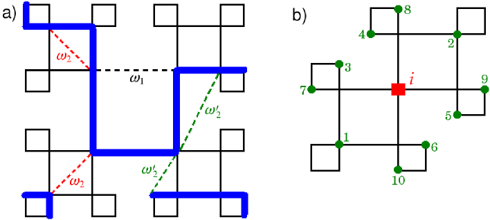
Figure 1: (Color online) a) Example of contribution to the partition function of the model on a Husimi tree with three generations. The polymer chains are represented by full thick (blue) lines and the dashed lines gives examples of each type of monomer interaction. The weight of this configuration is z18ω12ω28ω24superscript𝑧18superscriptsubscript𝜔12superscriptsubscript𝜔28superscriptsubscript𝜔24z^{18}\omega_{1}^{2}\omega_{2}^{8}\omega_{2}^{\prime 4}. b) Definition of the second neighbor (circles) - by the chemical distance - of the site i𝑖i (square).

We investigate interacting self- and mutually avoiding walks on a Husimi lattice - the core of a Cayley tree b82 - built with squares (see Fig.1). The endpoints of the walks are placed on the surface of the tree. In our grand-canonical solution, the thermodynamic variables of interest are the monomer fugacity z𝑧z and the Boltzmann weights ω1=exp(ϵ1/kBT)subscript𝜔1subscriptitalic-ϵ1subscript𝑘𝐵𝑇\omega_{1}=\exp(\epsilon_{1}/k_{B}T) and ω2=exp(ϵ2/kBT)subscript𝜔2subscriptitalic-ϵ2subscript𝑘𝐵𝑇\omega_{2}=\exp(\epsilon_{2}/k_{B}T) associated to each pair of nonconsecutive monomers on nearest-neighbor (NN) sites and pairs of monomers on next-NN (NNN) sites on the lattice, respectively. Hereafter, we will refer to them as NN and NNN monomers. Then, the grand-canonical partition function of the model is given by

Y=zMω1MNNω2MNNN,𝑌superscript𝑧𝑀superscriptsubscript𝜔1subscript𝑀𝑁𝑁superscriptsubscript𝜔2subscript𝑀𝑁𝑁𝑁Y=\sum z^{M}\omega_{1}^{M_{NN}}\omega_{2}^{M_{NNN}}, (1)

where the sum runs over all configurations of the walks on the tree, and M𝑀M, MNNsubscript𝑀𝑁𝑁M_{NN} and MNNNsubscript𝑀𝑁𝑁𝑁M_{NNN} are respectively the total number of monomers and the number of NN and NNN monomers. At this point, one notices that on the Husimi lattice there exists an ambiguity in definition of NNN sites:

a) the neighborhood of a given site, let us say i𝑖i, can be defined according to the chemical distance (associated to the number of steps along the lattice edges to reach a site j𝑗j starting at i𝑖i). So, at first, any site would have ten second neighbors, as shown in Fig. 1b. However, four of these sites (7-10 in Fig. 1b) would correspond to third neighbors on the square lattice. Since our aim is to compare the Husimi solution with results for the ordinary lattice, it is more reasonable to define only six NNN sites (the 1-6 ones in Fig. 1b).

b) Another option is to state that second neighbors are the sites in opposite vertices of an elementary square (sites 1-i𝑖i and 2-i𝑖i, in Fig. 1b). Then, each site will have two NNN ones.

Since definition a (b) - hereafter called approach A (C) - overestimates (underestimates) the number of second neighbors on square lattice - which is four -, both approaches will be analyzed in the following. It is easy to see in Fig. 1b that the overestimate in case A comes from the “out-square” sites 3-6, because in the ordinary lattice 3 and 4 (and also 5 and 6) would be a single site. So, this “excess” of second neighbors can be compensated by assigning only half of NNN energy (ϵ2/2subscriptitalic-ϵ22\epsilon_{2}/2) for “out-square” NNN monomers. In this way, the contribution to the partition function of the possible six NNN monomers will be effectively the same of four NNN ones (i.e., ω24superscriptsubscript𝜔24\omega_{2}^{4}). This case will be referred to as approach B. In order to consider all these cases in a general way, one may assign a weight ω2subscript𝜔2\omega_{2} for “in-square” NNN monomers and a weight ω2superscriptsubscript𝜔2\omega_{2}^{\prime} for the “out-square” NNN monomers (see Fig. 1a). Thence, the approaches A, B and C are recovered by making ω2=ω2superscriptsubscript𝜔2subscript𝜔2\omega_{2}^{\prime}=\omega_{2}, ω2=ω2superscriptsubscript𝜔2subscript𝜔2\omega_{2}^{\prime}=\sqrt{\omega_{2}} and ω2=1superscriptsubscript𝜔21\omega_{2}^{\prime}=1, respectively.

Refer to caption
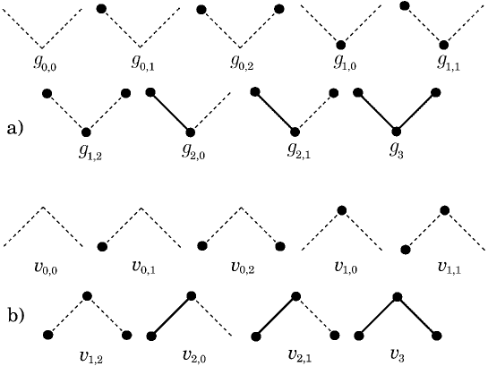
Figure 2: Definition of a) the root sites for each partial partition function and b) the types of possible vertices. Circles indicate the presence of monomers in the vertex and their bonds are represented by full lines.

A subtree with generation M+1𝑀1M+1 can be obtained by attaching 3 subtrees (each one with M𝑀M generations) in 3 vertices of an elementary square. The remaining vertex is usually called the “root site” and, associated to it, a partial partition function (ppf) gisubscript𝑔𝑖g_{i} is defined. Nine root sites and, thus, nine ppf’s are required to correctly account for the NNN interactions (see Fig. 2a). The ppf gisubscript𝑔𝑖g_{i} in generation M+1𝑀1M+1 is determined counting all possible configurations produced by attaching 3 subtrees (each one with M𝑀M generations) in a square with root site of type i𝑖i. Instead of do this directly, it is convenient to determine first the contribution coming from each type of vertex of the elementary square (depicted in Fig. 2b), being

v0,0=g0,0+2g0,1+g0,2,subscript𝑣00subscript𝑔002subscript𝑔01subscript𝑔02v_{0,0}=g_{0,0}+2g_{0,1}+g_{0,2}, (2a)
v0,1=g0,0+(1+ω2)g0,1+ω2g0,2,subscript𝑣01subscript𝑔001superscriptsubscript𝜔2subscript𝑔01superscriptsubscript𝜔2subscript𝑔02v_{0,1}=g_{0,0}+(1+\omega_{2}^{\prime})g_{0,1}+\omega_{2}^{\prime}g_{0,2}, (2b)
v0,2=g0,0+2ω2g0,1+ω22g0,2,subscript𝑣02subscript𝑔002superscriptsubscript𝜔2subscript𝑔01superscriptsubscript𝜔22subscript𝑔02v_{0,2}=g_{0,0}+2\omega_{2}^{\prime}g_{0,1}+\omega_{2}^{\prime 2}g_{0,2}, (2c)
v1,0=zg3,subscript𝑣10𝑧subscript𝑔3v_{1,0}=zg_{3}, (2d)
v1,1=zω2g3,subscript𝑣11𝑧superscriptsubscript𝜔2subscript𝑔3v_{1,1}=z\omega_{2}^{\prime}g_{3}, (2e)
v1,2=zω22g3,subscript𝑣12𝑧superscriptsubscript𝜔22subscript𝑔3v_{1,2}=z\omega_{2}^{\prime 2}g_{3}, (2f)
v2,0=z[(1+ω2)g2,0+2ω2g2,1],subscript𝑣20𝑧delimited-[]1superscriptsubscript𝜔2subscript𝑔202superscriptsubscript𝜔2subscript𝑔21v_{2,0}=z[(1+\omega_{2}^{\prime})g_{2,0}+2\omega_{2}^{\prime}g_{2,1}], (2g)
v2,1=2z(ω2g2,0+ω22g2,1),subscript𝑣212𝑧superscriptsubscript𝜔2subscript𝑔20superscriptsubscript𝜔22subscript𝑔21v_{2,1}=2z(\omega_{2}^{\prime}g_{2,0}+\omega_{2}^{\prime 2}g_{2,1}), (2h)
v3=z(g1,0+2ω2g1,1+ω22g1,2).subscript𝑣3𝑧subscript𝑔102superscriptsubscript𝜔2subscript𝑔11superscriptsubscript𝜔22subscript𝑔12v_{3}=z(g_{1,0}+2\omega_{2}^{\prime}g_{1,1}+\omega_{2}^{\prime 2}g_{1,2}). (2i)

In terms of these expressions, it is quite simple to determine the recursion relations for the ppf’s of the model, given by

g0,0=v0,03+v0,12v1,0,superscriptsubscript𝑔00superscriptsubscript𝑣003superscriptsubscript𝑣012subscript𝑣10g_{0,0}^{\prime}=v_{0,0}^{3}+v_{0,1}^{2}v_{1,0}, (3a)
g0,1=v0,0v0,1v1,0+ω1v0,1v1,12+v0,1v2,02,superscriptsubscript𝑔01subscript𝑣00subscript𝑣01subscript𝑣10subscript𝜔1subscript𝑣01superscriptsubscript𝑣112subscript𝑣01superscriptsubscript𝑣202g_{0,1}^{\prime}=v_{0,0}v_{0,1}v_{1,0}+\omega_{1}v_{0,1}v_{1,1}^{2}+v_{0,1}v_{2,0}^{2}, (3b)
g0,2=ω2[v0,2v1,02+ω12v1,12v1,2+2ω1v1,1v2,0v2,1+v2,02v3],superscriptsubscript𝑔02subscript𝜔2delimited-[]subscript𝑣02superscriptsubscript𝑣102superscriptsubscript𝜔12superscriptsubscript𝑣112subscript𝑣122subscript𝜔1subscript𝑣11subscript𝑣20subscript𝑣21superscriptsubscript𝑣202subscript𝑣3g_{0,2}^{\prime}=\omega_{2}[v_{0,2}v_{1,0}^{2}+\omega_{1}^{2}v_{1,1}^{2}v_{1,2}+2\omega_{1}v_{1,1}v_{2,0}v_{2,1}+v_{2,0}^{2}v_{3}], (3c)
g1,0=v0,0v0,12+ω2v0,22v1,0,superscriptsubscript𝑔10subscript𝑣00superscriptsubscript𝑣012subscript𝜔2superscriptsubscript𝑣022subscript𝑣10g_{1,0}^{\prime}=v_{0,0}v_{0,1}^{2}+\omega_{2}v_{0,2}^{2}v_{1,0}, (3d)
g1,1=ω1[v0,12v1,1+ω1ω2v0,2v1,1v1,2+ω2v0,2v2,0v2,1],superscriptsubscript𝑔11subscript𝜔1delimited-[]superscriptsubscript𝑣012subscript𝑣11subscript𝜔1subscript𝜔2subscript𝑣02subscript𝑣11subscript𝑣12subscript𝜔2subscript𝑣02subscript𝑣20subscript𝑣21g_{1,1}^{\prime}=\omega_{1}[v_{0,1}^{2}v_{1,1}+\omega_{1}\omega_{2}v_{0,2}v_{1,1}v_{1,2}+\omega_{2}v_{0,2}v_{2,0}v_{2,1}], (3e)
g1,2=ω12ω2[v0,2v1,12+ω12ω2v1,23+2ω1ω2v1,2v2,12+ω2v2,12v3],superscriptsubscript𝑔12superscriptsubscript𝜔12subscript𝜔2delimited-[]subscript𝑣02superscriptsubscript𝑣112superscriptsubscript𝜔12subscript𝜔2superscriptsubscript𝑣1232subscript𝜔1subscript𝜔2subscript𝑣12superscriptsubscript𝑣212subscript𝜔2superscriptsubscript𝑣212subscript𝑣3g_{1,2}^{\prime}=\omega_{1}^{2}\omega_{2}[v_{0,2}v_{1,1}^{2}+\omega_{1}^{2}\omega_{2}v_{1,2}^{3}+2\omega_{1}\omega_{2}v_{1,2}v_{2,1}^{2}+\omega_{2}v_{2,1}^{2}v_{3}], (3f)
g2,0=v0,12v2,0+ω1ω2v0,2v1,1v2,1+ω2v0,2v2,0v3,superscriptsubscript𝑔20superscriptsubscript𝑣012subscript𝑣20subscript𝜔1subscript𝜔2subscript𝑣02subscript𝑣11subscript𝑣21subscript𝜔2subscript𝑣02subscript𝑣20subscript𝑣3g_{2,0}^{\prime}=v_{0,1}^{2}v_{2,0}+\omega_{1}\omega_{2}v_{0,2}v_{1,1}v_{2,1}+\omega_{2}v_{0,2}v_{2,0}v_{3}, (3g)
g2,1=ω1ω2[v0,2v1,1v2,0+ω12ω2v1,22v2,1+ω1ω2(v2,13+v1,2v2,1v3)+ω2v2,1v32],superscriptsubscript𝑔21subscript𝜔1subscript𝜔2delimited-[]subscript𝑣02subscript𝑣11subscript𝑣20superscriptsubscript𝜔12subscript𝜔2superscriptsubscript𝑣122subscript𝑣21subscript𝜔1subscript𝜔2superscriptsubscript𝑣213subscript𝑣12subscript𝑣21subscript𝑣3subscript𝜔2subscript𝑣21superscriptsubscript𝑣32g_{2,1}^{\prime}=\omega_{1}\omega_{2}[v_{0,2}v_{1,1}v_{2,0}+\omega_{1}^{2}\omega_{2}v_{1,2}^{2}v_{2,1}+\omega_{1}\omega_{2}(v_{2,1}^{3}+v_{1,2}v_{2,1}v_{3})+\omega_{2}v_{2,1}v_{3}^{2}], (3h)
g3=ω2[v0,2v2,02+ω12ω2v1,2v2,12+2ω1ω2v2,12v3],superscriptsubscript𝑔3subscript𝜔2delimited-[]subscript𝑣02superscriptsubscript𝑣202superscriptsubscript𝜔12subscript𝜔2subscript𝑣12superscriptsubscript𝑣2122subscript𝜔1subscript𝜔2superscriptsubscript𝑣212subscript𝑣3g_{3}^{\prime}=\omega_{2}[v_{0,2}v_{2,0}^{2}+\omega_{1}^{2}\omega_{2}v_{1,2}v_{2,1}^{2}+2\omega_{1}\omega_{2}v_{2,1}^{2}v_{3}], (3i)

where gisubscript𝑔𝑖g_{i} and gisuperscriptsubscript𝑔𝑖g_{i}^{\prime} are in generations M𝑀M and M+1𝑀1M+1, respectively.

In a similar way, the partition function of the model on the Cayley tree can be find by attaching four subtrees in a central square, which yields

Y𝑌\displaystyle Y =\displaystyle= v0,04+4v0,0v0,12v1,0+4ω1v0,12v1,12+2ω2v0,22v1,02+4ω12ω2v0,2v1,12v1,2+ω14ω22v1,24+4v0,12v2,02superscriptsubscript𝑣0044subscript𝑣00superscriptsubscript𝑣012subscript𝑣104subscript𝜔1superscriptsubscript𝑣012superscriptsubscript𝑣1122subscript𝜔2superscriptsubscript𝑣022superscriptsubscript𝑣1024superscriptsubscript𝜔12subscript𝜔2subscript𝑣02superscriptsubscript𝑣112subscript𝑣12superscriptsubscript𝜔14superscriptsubscript𝜔22superscriptsubscript𝑣1244superscriptsubscript𝑣012superscriptsubscript𝑣202\displaystyle v_{0,0}^{4}+4v_{0,0}v_{0,1}^{2}v_{1,0}+4\omega_{1}v_{0,1}^{2}v_{1,1}^{2}+2\omega_{2}v_{0,2}^{2}v_{1,0}^{2}+4\omega_{1}^{2}\omega_{2}v_{0,2}v_{1,1}^{2}v_{1,2}+\omega_{1}^{4}\omega_{2}^{2}v_{1,2}^{4}+4v_{0,1}^{2}v_{2,0}^{2}
+\displaystyle+ 8ω1ω2v0,2v1,1v2,0v2,1+4ω2v0,2v2,02v3+4ω13ω22v1,22v2,12+2ω12ω22(v2,14+2v1,2v2,12v3)+4ω1ω22v2,12v32.8subscript𝜔1subscript𝜔2subscript𝑣02subscript𝑣11subscript𝑣20subscript𝑣214subscript𝜔2subscript𝑣02superscriptsubscript𝑣202subscript𝑣34superscriptsubscript𝜔13superscriptsubscript𝜔22superscriptsubscript𝑣122superscriptsubscript𝑣2122superscriptsubscript𝜔12superscriptsubscript𝜔22superscriptsubscript𝑣2142subscript𝑣12superscriptsubscript𝑣212subscript𝑣34subscript𝜔1superscriptsubscript𝜔22superscriptsubscript𝑣212superscriptsubscript𝑣32\displaystyle 8\omega_{1}\omega_{2}v_{0,2}v_{1,1}v_{2,0}v_{2,1}+4\omega_{2}v_{0,2}v_{2,0}^{2}v_{3}+4\omega_{1}^{3}\omega_{2}^{2}v_{1,2}^{2}v_{2,1}^{2}+2\omega_{1}^{2}\omega_{2}^{2}(v_{2,1}^{4}+2v_{1,2}v_{2,1}^{2}v_{3})+4\omega_{1}\omega_{2}^{2}v_{2,1}^{2}v_{3}^{2}.

Then, the densities of monomers (ρ𝜌\rho), of NN (ρNNsubscript𝜌𝑁𝑁\rho_{NN}) and NNN (ρNNNsubscript𝜌𝑁𝑁𝑁\rho_{NNN}) monomers are

ρ=z4Y(Yz),ρNN=ω14Y(Yω1)andρNNN=ω2SY(Yω2),formulae-sequence𝜌𝑧4𝑌𝑌𝑧formulae-sequencesubscript𝜌𝑁𝑁subscript𝜔14𝑌𝑌subscript𝜔1andsubscript𝜌𝑁𝑁𝑁subscript𝜔2𝑆𝑌𝑌subscript𝜔2\rho=\frac{z}{4Y}\left(\frac{\partial Y}{\partial z}\right),\quad\quad\rho_{NN}=\frac{\omega_{1}}{4Y}\left(\frac{\partial Y}{\partial\omega_{1}}\right)\quad\quad\text{and}\quad\quad\rho_{NNN}=\frac{\omega_{2}}{SY}\left(\frac{\partial Y}{\partial\omega_{2}}\right), (5)

where S=10𝑆10S=10, 666 and 222 are used in approaches A, B and C, respectively, to make the maximum value of ρNNNsubscript𝜌𝑁𝑁𝑁\rho_{NNN} equal 1 in all cases.

In the thermodynamic limit, when the number of generations of the tree and, consequently, the length of the polymers tend to infinity, the ppf’s diverge, so, we will work with ratios of them, defined as R1=g0,1/g0,0subscript𝑅1subscript𝑔01subscript𝑔00R_{1}=g_{0,1}/g_{0,0}, R2=g0,2/g0,0subscript𝑅2subscript𝑔02subscript𝑔00R_{2}=g_{0,2}/g_{0,0}, R3=g1,0/g0,0subscript𝑅3subscript𝑔10subscript𝑔00R_{3}=g_{1,0}/g_{0,0}, R4=g1,1/g0,0subscript𝑅4subscript𝑔11subscript𝑔00R_{4}=g_{1,1}/g_{0,0}, R5=g1,2/g0,0subscript𝑅5subscript𝑔12subscript𝑔00R_{5}=g_{1,2}/g_{0,0}, R6=g2,0/g0,0subscript𝑅6subscript𝑔20subscript𝑔00R_{6}=g_{2,0}/g_{0,0}, R7=g2,1/g0,0subscript𝑅7subscript𝑔21subscript𝑔00R_{7}=g_{2,1}/g_{0,0} and R8=g3/g0,0subscript𝑅8subscript𝑔3subscript𝑔00R_{8}=g_{3}/g_{0,0}. This leads to the recursion relations (RR’s):

R1=(zABR8+z2ω1ω22αBR82+z2BD2)/R0,superscriptsubscript𝑅1𝑧𝐴𝐵subscript𝑅8superscript𝑧2subscript𝜔1superscriptsubscript𝜔22𝛼𝐵superscriptsubscript𝑅82superscript𝑧2𝐵superscript𝐷2subscript𝑅0R_{1}^{\prime}=(zABR_{8}+z^{2}\omega_{1}\omega_{2}^{2\alpha}BR_{8}^{2}+z^{2}BD^{2})/R_{0}, (6a)
R2=ω2(z2CR82+z3ω12ω24αR83+4z3ω1ω2αDER8+z3D2F)/R0,subscriptsuperscript𝑅2subscript𝜔2superscript𝑧2𝐶superscriptsubscript𝑅82superscript𝑧3superscriptsubscript𝜔12superscriptsubscript𝜔24𝛼superscriptsubscript𝑅834superscript𝑧3subscript𝜔1superscriptsubscript𝜔2𝛼𝐷𝐸subscript𝑅8superscript𝑧3superscript𝐷2𝐹subscript𝑅0R^{\prime}_{2}=\omega_{2}(z^{2}CR_{8}^{2}+z^{3}\omega_{1}^{2}\omega_{2}^{4\alpha}R_{8}^{3}+4z^{3}\omega_{1}\omega_{2}^{\alpha}DER_{8}+z^{3}D^{2}F)/R_{0}, (6b)
R3=(AB2+zω2C2R8)/R0,subscriptsuperscript𝑅3𝐴superscript𝐵2𝑧subscript𝜔2superscript𝐶2subscript𝑅8subscript𝑅0\displaystyle R^{\prime}_{3}=(AB^{2}+z\omega_{2}C^{2}R_{8})/R_{0},
R4=ω1(zω2αB2R8+z2ω1ω23α+1CR82+2z2ω2CDE)/R0,subscriptsuperscript𝑅4subscript𝜔1𝑧superscriptsubscript𝜔2𝛼superscript𝐵2subscript𝑅8superscript𝑧2subscript𝜔1superscriptsubscript𝜔23𝛼1𝐶superscriptsubscript𝑅822superscript𝑧2subscript𝜔2𝐶𝐷𝐸subscript𝑅0R^{\prime}_{4}=\omega_{1}(z\omega_{2}^{\alpha}B^{2}R_{8}+z^{2}\omega_{1}\omega_{2}^{3\alpha+1}CR_{8}^{2}+2z^{2}\omega_{2}CDE)/R_{0}, (6c)
R5=ω12ω2(z2ω22αCR82+z3ω12ω26α+1R83+8z3ω1ω22α+1E2R8+4z3ω2E2F)/R0,subscriptsuperscript𝑅5superscriptsubscript𝜔12subscript𝜔2superscript𝑧2superscriptsubscript𝜔22𝛼𝐶superscriptsubscript𝑅82superscript𝑧3superscriptsubscript𝜔12superscriptsubscript𝜔26𝛼1superscriptsubscript𝑅838superscript𝑧3subscript𝜔1superscriptsubscript𝜔22𝛼1superscript𝐸2subscript𝑅84superscript𝑧3subscript𝜔2superscript𝐸2𝐹subscript𝑅0R^{\prime}_{5}=\omega_{1}^{2}\omega_{2}(z^{2}\omega_{2}^{2\alpha}CR_{8}^{2}+z^{3}\omega_{1}^{2}\omega_{2}^{6\alpha+1}R_{8}^{3}+8z^{3}\omega_{1}\omega_{2}^{2\alpha+1}E^{2}R_{8}+4z^{3}\omega_{2}E^{2}F)/R_{0}, (6d)
R6=(zB2D+2z2ω1ω2α+1CER8+z2ω2CDF)/R0,subscriptsuperscript𝑅6𝑧superscript𝐵2𝐷2superscript𝑧2subscript𝜔1superscriptsubscript𝜔2𝛼1𝐶𝐸subscript𝑅8superscript𝑧2subscript𝜔2𝐶𝐷𝐹subscript𝑅0R^{\prime}_{6}=(zB^{2}D+2z^{2}\omega_{1}\omega_{2}^{\alpha+1}CER_{8}+z^{2}\omega_{2}CDF)/R_{0}, (6e)
R7=ω1ω2[z2ω2αCDR8+2z3ω12ω24α+1ER82+ω1ω2(8z3E3+2z3ω22αEFR8)+2z3ω2EF2]/R0,subscriptsuperscript𝑅7subscript𝜔1subscript𝜔2delimited-[]superscript𝑧2superscriptsubscript𝜔2𝛼𝐶𝐷subscript𝑅82superscript𝑧3superscriptsubscript𝜔12superscriptsubscript𝜔24𝛼1𝐸superscriptsubscript𝑅82subscript𝜔1subscript𝜔28superscript𝑧3superscript𝐸32superscript𝑧3superscriptsubscript𝜔22𝛼𝐸𝐹subscript𝑅82superscript𝑧3subscript𝜔2𝐸superscript𝐹2subscript𝑅0R^{\prime}_{7}=\omega_{1}\omega_{2}[z^{2}\omega_{2}^{\alpha}CDR_{8}+2z^{3}\omega_{1}^{2}\omega_{2}^{4\alpha+1}ER_{8}^{2}+\omega_{1}\omega_{2}(8z^{3}E^{3}+2z^{3}\omega_{2}^{2\alpha}EFR_{8})+2z^{3}\omega_{2}EF^{2}]/R_{0}, (6f)
R8=ω2(z2CD2+4z3ω12ω22α+1E2R8+8z3ω1ω2E2F)/R0,subscriptsuperscript𝑅8subscript𝜔2superscript𝑧2𝐶superscript𝐷24superscript𝑧3superscriptsubscript𝜔12superscriptsubscript𝜔22𝛼1superscript𝐸2subscript𝑅88superscript𝑧3subscript𝜔1subscript𝜔2superscript𝐸2𝐹subscript𝑅0R^{\prime}_{8}=\omega_{2}(z^{2}CD^{2}+4z^{3}\omega_{1}^{2}\omega_{2}^{2\alpha+1}E^{2}R_{8}+8z^{3}\omega_{1}\omega_{2}E^{2}F)/R_{0}, (6g)
with
R0=(1+2R1+R2)3+z[1+(1+ω2α)R1+ω2αR2]2R8,subscript𝑅0superscript12subscript𝑅1subscript𝑅23𝑧superscriptdelimited-[]11superscriptsubscript𝜔2𝛼subscript𝑅1superscriptsubscript𝜔2𝛼subscript𝑅22subscript𝑅8R_{0}=(1+2R_{1}+R_{2})^{3}+z[1+(1+\omega_{2}^{\alpha})R_{1}+\omega_{2}^{\alpha}R_{2}]^{2}R_{8}, (6h)
A=1+2R1+R2,𝐴12subscript𝑅1subscript𝑅2A=1+2R_{1}+R_{2}, (6i)
B=1+(1+ω2α)R1+ω2αR2,𝐵11superscriptsubscript𝜔2𝛼subscript𝑅1superscriptsubscript𝜔2𝛼subscript𝑅2B=1+(1+\omega_{2}^{\alpha})R_{1}+\omega_{2}^{\alpha}R_{2}, (6j)
C=1+2ω2αR1+ω22αR2,𝐶12superscriptsubscript𝜔2𝛼subscript𝑅1superscriptsubscript𝜔22𝛼subscript𝑅2C=1+2\omega_{2}^{\alpha}R_{1}+\omega_{2}^{2\alpha}R_{2}, (6k)
D=(1+ω2α)R6+2ω2αR7,𝐷1superscriptsubscript𝜔2𝛼subscript𝑅62superscriptsubscript𝜔2𝛼subscript𝑅7D=(1+\omega_{2}^{\alpha})R_{6}+2\omega_{2}^{\alpha}R_{7}, (6l)
E=ω2αR6+ω22αR7,𝐸superscriptsubscript𝜔2𝛼subscript𝑅6superscriptsubscript𝜔22𝛼subscript𝑅7E=\omega_{2}^{\alpha}R_{6}+\omega_{2}^{2\alpha}R_{7}, (6m)
F=R3+2ω2αR4+ω22αR5,𝐹subscript𝑅32superscriptsubscript𝜔2𝛼subscript𝑅4superscriptsubscript𝜔22𝛼subscript𝑅5F=R_{3}+2\omega_{2}^{\alpha}R_{4}+\omega_{2}^{2\alpha}R_{5}, (6n)

where α=1𝛼1\alpha=1, 1/2121/2 and 00 in cases A, B and C, respectively. In the case C (ω2=1superscriptsubscript𝜔21\omega_{2}^{\prime}=1), it is easy to see that v0,0=v0,1=v0,2=(g0,0+2g0,1+g0,2)subscript𝑣00subscript𝑣01subscript𝑣02subscript𝑔002subscript𝑔01subscript𝑔02v_{0,0}=v_{0,1}=v_{0,2}=(g_{0,0}+2g_{0,1}+g_{0,2}), v1,0=v1,1=v1,2=zg3subscript𝑣10subscript𝑣11subscript𝑣12𝑧subscript𝑔3v_{1,0}=v_{1,1}=v_{1,2}=zg_{3}, v2,0=v2,1=2z(g2,0+g2,1)subscript𝑣20subscript𝑣212𝑧subscript𝑔20subscript𝑔21v_{2,0}=v_{2,1}=2z(g_{2,0}+g_{2,1}) and v3=z(g1,0+2g1,1+g1,2)subscript𝑣3𝑧subscript𝑔102subscript𝑔11subscript𝑔12v_{3}=z(g_{1,0}+2g_{1,1}+g_{1,2}) and, thus, only the combinations g0(g0,0+2g0,1+g0,2)subscript𝑔0subscript𝑔002subscript𝑔01subscript𝑔02g_{0}\equiv(g_{0,0}+2g_{0,1}+g_{0,2}), g1(g1,0+2g1,1+g1,2)subscript𝑔1subscript𝑔102subscript𝑔11subscript𝑔12g_{1}\equiv(g_{1,0}+2g_{1,1}+g_{1,2}) and g2(g2,0+g2,1)subscript𝑔2subscript𝑔20subscript𝑔21g_{2}\equiv(g_{2,0}+g_{2,1}) will appear in the recursion relations. Thus, one may work with simplified ratios of ppf’s, defined as R1=g1/g0subscript𝑅1subscript𝑔1subscript𝑔0R_{1}=g_{1}/g_{0}, R2=g2/g0subscript𝑅2subscript𝑔2subscript𝑔0R_{2}=g_{2}/g_{0} and R3=g3/g0subscript𝑅3subscript𝑔3subscript𝑔0R_{3}=g_{3}/g_{0}, yielding

R1=[1+z(2ω1+ω2)R3+3z2ω12ω2R32+z3ω14ω22R33+8z2ω1ω2R22+8z3ω13ω22R22R3+4z3ω12ω22R1R22]/R0,superscriptsubscript𝑅1delimited-[]1𝑧2subscript𝜔1subscript𝜔2subscript𝑅33superscript𝑧2superscriptsubscript𝜔12subscript𝜔2superscriptsubscript𝑅32superscript𝑧3superscriptsubscript𝜔14superscriptsubscript𝜔22superscriptsubscript𝑅338superscript𝑧2subscript𝜔1subscript𝜔2superscriptsubscript𝑅228superscript𝑧3superscriptsubscript𝜔13superscriptsubscript𝜔22superscriptsubscript𝑅22subscript𝑅34superscript𝑧3superscriptsubscript𝜔12superscriptsubscript𝜔22subscript𝑅1superscriptsubscript𝑅22subscript𝑅0R_{1}^{\prime}=[1+z(2\omega_{1}+\omega_{2})R_{3}+3z^{2}\omega_{1}^{2}\omega_{2}R_{3}^{2}+z^{3}\omega_{1}^{4}\omega_{2}^{2}R_{3}^{3}+8z^{2}\omega_{1}\omega_{2}R_{2}^{2}+8z^{3}\omega_{1}^{3}\omega_{2}^{2}R_{2}^{2}R_{3}+4z^{3}\omega_{1}^{2}\omega_{2}^{2}R_{1}R_{2}^{2}]/R_{0}, (7a)
R2=2zR2(1+2zω1ω2R3+z2ω13ω22R32+4z2ω12ω22R22+zω2R1+z2ω12ω22R1R3+z2ω1ω22R12)/R0,superscriptsubscript𝑅22𝑧subscript𝑅212𝑧subscript𝜔1subscript𝜔2subscript𝑅3superscript𝑧2superscriptsubscript𝜔13superscriptsubscript𝜔22superscriptsubscript𝑅324superscript𝑧2superscriptsubscript𝜔12superscriptsubscript𝜔22superscriptsubscript𝑅22𝑧subscript𝜔2subscript𝑅1superscript𝑧2superscriptsubscript𝜔12superscriptsubscript𝜔22subscript𝑅1subscript𝑅3superscript𝑧2subscript𝜔1superscriptsubscript𝜔22superscriptsubscript𝑅12subscript𝑅0R_{2}^{\prime}=2zR_{2}(1+2z\omega_{1}\omega_{2}R_{3}+z^{2}\omega_{1}^{3}\omega_{2}^{2}R_{3}^{2}+4z^{2}\omega_{1}^{2}\omega_{2}^{2}R_{2}^{2}+z\omega_{2}R_{1}+z^{2}\omega_{1}^{2}\omega_{2}^{2}R_{1}R_{3}+z^{2}\omega_{1}\omega_{2}^{2}R_{1}^{2})/R_{0}, (7b)
R3=4z2R22ω2(1+zω12ω2R3+2zω1ω2R1)/R0,superscriptsubscript𝑅34superscript𝑧2superscriptsubscript𝑅22subscript𝜔21𝑧superscriptsubscript𝜔12subscript𝜔2subscript𝑅32𝑧subscript𝜔1subscript𝜔2subscript𝑅1subscript𝑅0R_{3}^{\prime}=4z^{2}R_{2}^{2}\omega_{2}(1+z\omega_{1}^{2}\omega_{2}R_{3}+2z\omega_{1}\omega_{2}R_{1})/R_{0}, (7c)
with
R0=1+3zR3+z2(2ω1+ω2)R32+z3ω12ω2R33+8z2R22+8z3ω1ω2R22R3+4z3ω2R1R22subscript𝑅013𝑧subscript𝑅3superscript𝑧22subscript𝜔1subscript𝜔2superscriptsubscript𝑅32superscript𝑧3superscriptsubscript𝜔12subscript𝜔2superscriptsubscript𝑅338superscript𝑧2superscriptsubscript𝑅228superscript𝑧3subscript𝜔1subscript𝜔2superscriptsubscript𝑅22subscript𝑅34superscript𝑧3subscript𝜔2subscript𝑅1superscriptsubscript𝑅22R_{0}=1+3zR_{3}+z^{2}(2\omega_{1}+\omega_{2})R_{3}^{2}+z^{3}\omega_{1}^{2}\omega_{2}R_{3}^{3}+8z^{2}R_{2}^{2}+8z^{3}\omega_{1}\omega_{2}R_{2}^{2}R_{3}+4z^{3}\omega_{2}R_{1}R_{2}^{2} (7d)

It is worth noting that the partition functions (Eq. II) for approach X𝑋X, with X=𝑋absentX=A, B or C, can be written as YX=g0,04yXsubscript𝑌𝑋superscriptsubscript𝑔004subscript𝑦𝑋Y_{X}=g_{0,0}^{4}y_{X}, where yXsubscript𝑦𝑋y_{X} is finite (since is depends only on the ratios Risubscript𝑅𝑖R_{i}, beyond z𝑧z, ω1subscript𝜔1\omega_{1} and ω2subscript𝜔2\omega_{2}), while YXsubscript𝑌𝑋Y_{X} diverges as g0,04superscriptsubscript𝑔004g_{0,0}^{4}, in the thermodynamic limit. Notwithstanding, the densities (Eq. 5) remain finite because they are in fact functions of yXsubscript𝑦𝑋y_{X}, instead of YXsubscript𝑌𝑋Y_{X}.

III Thermodynamic properties of model

The thermodynamic phases of the model on the Husimi lattice are given by the real and positive fixed points of the recursion relations (RR’s - Eqs. 6). Similarly to the classical ISAW model (ω2=1subscript𝜔21\omega_{2}=1), the grand-canonical phase diagram for general ω2subscript𝜔2\omega_{2} presents only two phases: i) a non-polymerized (NP) phase, where R3=1subscript𝑅31R_{3}=1 and Ri=0subscript𝑅𝑖0R_{i}=0 otherwise; and ii) a polymerized (P) phase, with Ri0subscript𝑅𝑖0R_{i}\neq 0 for i=1,,8𝑖18i=1,\ldots,8. In the former, the density of monomers vanishes (ρ=0𝜌0\rho=0) and, consequently, ρNN=ρNNN=0subscript𝜌𝑁𝑁subscript𝜌𝑁𝑁𝑁0\rho_{NN}=\rho_{NNN}=0. On the other hand, in P phase these densities are, in general, non-null and depend on the parameters z𝑧z, ω1subscript𝜔1\omega_{1} and ω2subscript𝜔2\omega_{2}. Obviously, working with the reduced set of RR’s (Eqs. 7) in approach C, one finds a similar behavior, with R1=1subscript𝑅11R_{1}=1, R2=R3=0subscript𝑅2subscript𝑅30R_{2}=R_{3}=0 in NP phase, and Ri0subscript𝑅𝑖0R_{i}\neq 0 in P one.

Each phase is stable in the region of the parameter space (z,ω1,ω2𝑧subscript𝜔1subscript𝜔2z,\omega_{1},\omega_{2}) where the largest eigenvalue λ𝜆\lambda of its Jacobian matrix (Ji,j=RiRj)subscript𝐽𝑖𝑗subscriptsuperscript𝑅𝑖subscript𝑅𝑗\left(J_{i,j}=\frac{\partial R^{\prime}_{i}}{\partial R_{j}}\right) is smaller than one. The condition λ=1𝜆1\lambda=1 gives the thermodynamic stability limit (the spinodal) of the respective phase, which is easy to calculate in NP phase, being

ω1=12z3ω22(α+1)(1+z+zω2α+z2ω2+z2ω2α+11z+zω2αz2ω2+z2ω2α+1),subscript𝜔112superscript𝑧3superscriptsubscript𝜔22𝛼11𝑧𝑧superscriptsubscript𝜔2𝛼superscript𝑧2subscript𝜔2superscript𝑧2superscriptsubscript𝜔2𝛼11𝑧𝑧superscriptsubscript𝜔2𝛼superscript𝑧2subscript𝜔2superscript𝑧2superscriptsubscript𝜔2𝛼1\omega_{1}=\frac{1}{2z^{3}\omega_{2}^{2(\alpha+1)}}\left(\frac{-1+z+z\omega_{2}^{\alpha}+z^{2}\omega_{2}+z^{2}\omega_{2}^{\alpha+1}}{-1-z+z\omega_{2}^{\alpha}-z^{2}\omega_{2}+z^{2}\omega_{2}^{\alpha+1}}\right), (8)

recalling that α=1𝛼1\alpha=1, 1/2121/2 and 00 in approaches A, B and C, respectively. For the polymerized phase, the stability limit is determined numerically. In a certain region of the phase diagram, the NP and P spinodals are coincident, forming a critical surface.

There exists also a coexistence region in the phase diagram - where the spinodals do not match and both phases are stable - with a coexistence surface separating the NP and P phases there. A simple way to determine this surface is through the free energy of the model, which can be calculated using Gujrati’s prescription Gujrati . The derivation of this free energy for the Husimi lattice built with squares is presented in appendix A, leading to

ϕb=12(2lnR0,XlnyX)subscriptitalic-ϕ𝑏122subscript𝑅0𝑋subscript𝑦𝑋\phi_{b}=-\dfrac{1}{2}\left(2\ln R_{0,X}-\ln y_{X}\right) (9)

with X=𝑋absentX=A, B or C, and R0,Xsubscript𝑅0𝑋R_{0,X} and yXsubscript𝑦𝑋y_{X} defined as above and calculated at the fixed point. In NP phase, R0,X=yX=1subscript𝑅0𝑋subscript𝑦𝑋1R_{0,X}=y_{X}=1, so that ϕbNP=0superscriptsubscriptitalic-ϕ𝑏𝑁𝑃0\phi_{b}^{NP}=0 and, then, the coexistence surface - where the free energies of both phases are equal - is given by ϕbP=ϕbNP=0superscriptsubscriptitalic-ϕ𝑏𝑃superscriptsubscriptitalic-ϕ𝑏𝑁𝑃0\phi_{b}^{P}=\phi_{b}^{NP}=0.

These critical and coexistence surfaces meet (tangentially) at a tricritical (TC) line, which was calculated exactly by locating the points along the spinodal of NP phase where the solution of the RR’s is triply degenerate. This is demonstrated in detail in appendix B.
Refer to caption
Refer to caption
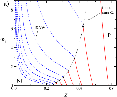
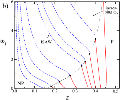
Figure 3: (Color online) Phase diagrams in the variables ω1subscript𝜔1\omega_{1} versus z𝑧z for approaches a) A and b) C. In a) diagrams for ω2subscript𝜔2\omega_{2} varying by 0.20.20.2 in the range [0.4,2.2]0.42.2[0.4,2.2] ω2=0.4,0.6,0.8,1.0,1.6,2.2,2.8,3.4subscript𝜔20.40.60.81.01.62.22.83.4\omega_{2}=0.4,0.6,0.8,1.0,1.6,2.2,2.8,3.4 and 4.04.04.0 are shown, while in b) they are for ω2=0.2,0.4,0.6,0.8,1.0,2.0,4.0,8.0subscript𝜔20.20.40.60.81.02.04.08.0\omega_{2}=0.2,0.4,0.6,0.8,1.0,2.0,4.0,8.0 and 16.016.016.0. The full (red) and dashed (blue) lines are the critical and coexistence lines, respectively. The black dots indicate the θ𝜃\theta points and the θ𝜃\theta line is given by the dotted (black) line.

Let us first discuss the thermodynamic behavior for approach A. Figure 3a shows phase diagrams for several values of (fixed) ω2subscript𝜔2\omega_{2} in the range [0.4,2.2]0.42.2[0.4,2.2]. For any ω2<1.9217692subscript𝜔21.9217692\omega_{2}<1.9217692, the same properties of the classical ISAW model (ω2=1subscript𝜔21\omega_{2}=1) are found: there is a continuous NP-P transition at small ω1subscript𝜔1\omega_{1} that becomes discontinuous at a tricritical (θ𝜃\theta) point. The location of the θ𝜃\theta point, however, strongly depends on ω2subscript𝜔2\omega_{2}, forming a continuous θ𝜃\theta-line.

In general, a decrease in the coordinates (zθ,ω1θsuperscript𝑧𝜃superscriptsubscript𝜔1𝜃z^{\theta},\omega_{1}^{\theta}) of the tricritical point is observed as ω2subscript𝜔2\omega_{2} increases. In fact, for attractive forces between NN and NNN monomers, this is quite expected, since βϵ2>0𝛽subscriptitalic-ϵ20\beta\epsilon_{2}>0 will facilitate the collapse and, thus, βϵ1𝛽subscriptitalic-ϵ1\beta\epsilon_{1} becomes smaller. When ω2=1.1553956subscript𝜔21.1553956\omega_{2}=1.1553956, the NN energy is null, i.e., ω1θ=1superscriptsubscript𝜔1𝜃1\omega_{1}^{\theta}=1 (and zθ=0.3085453superscript𝑧𝜃0.3085453z^{\theta}=0.3085453), so that the collapse transition happens due solely to the NNN interaction. For larger ω2subscript𝜔2\omega_{2}, the θ𝜃\theta-line still exists, but for ω1θ<1superscriptsubscript𝜔1𝜃1\omega_{1}^{\theta}<1, meaning that NN monomers repel each other. The value of ω1θsuperscriptsubscript𝜔1𝜃\omega_{1}^{\theta} decreases, for increasing ω2subscript𝜔2\omega_{2}, until reaches the zero at ω2=1.9217692subscript𝜔21.9217692\omega_{2}=1.9217692. Therefore, even for an infinite repulsive force between NN monomers a coil-globule transition exists for a finite (attractive) interaction between NNN ones. This will be discussed in more detail in the following. For ω2>1.9217692subscript𝜔21.9217692\omega_{2}>1.9217692, only a NP-P coexistence surface is found.

The θ𝜃\theta-line extends also to the region of repulsive NNN interactions (ω2<1subscript𝜔21\omega_{2}<1), where, again, increasing zθsuperscript𝑧𝜃z^{\theta} and ω1θsuperscriptsubscript𝜔1𝜃\omega_{1}^{\theta} are observed as ω2subscript𝜔2\omega_{2} decreases. When ω2subscript𝜔2\omega_{2} approaches the zero, one finds ω1θsuperscriptsubscript𝜔1𝜃\omega_{1}^{\theta}\rightarrow\infty and zθ1superscript𝑧𝜃1z^{\theta}\rightarrow 1. This is quite reasonable, since ω21much-less-thansubscript𝜔21\omega_{2}\ll 1 will prevent the formation of bends in the walks and, consequently, of a globular phase. Notwithstanding, if ω11much-greater-thansubscript𝜔11\omega_{1}\gg 1 the attractive NN force can overcome the NNN repulsion yielding this phase.

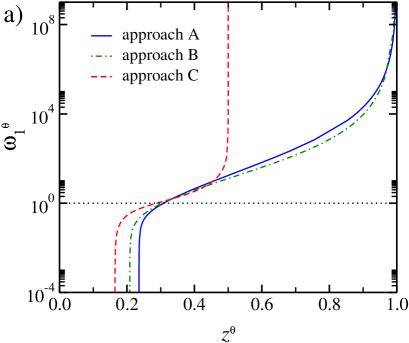
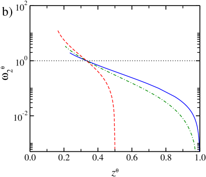
The phase diagram for approach C is presented in Fig. 3b, where the same qualitative behavior of A is observed, with θ𝜃\theta-lines extending also over the whole phase diagrams since ω1=0subscript𝜔10\omega_{1}=0 until ω1subscript𝜔1\omega_{1}\rightarrow\infty. An analogous phase diagram is also found for the intermediate approach B (not shown). These similarities are more evident in the comparison of the θ𝜃\theta-lines, for all approaches, which is presented in Fig. 4. In case A (B), the θ𝜃\theta-line starts at zθ=0.235592superscript𝑧𝜃0.235592z^{\theta}=0.235592 (0.2083040.2083040.208304) - where ω1θ=0superscriptsubscript𝜔1𝜃0\omega_{1}^{\theta}=0 and ω2θ=1.921769superscriptsubscript𝜔2𝜃1.921769\omega_{2}^{\theta}=1.921769 (3.3455813.3455813.345581) - and ends at zθ1superscript𝑧𝜃1z^{\theta}\rightarrow 1 - where ω1θsuperscriptsubscript𝜔1𝜃\omega_{1}^{\theta}\rightarrow\infty and ω2θ0superscriptsubscript𝜔2𝜃0\omega_{2}^{\theta}\rightarrow 0. On the other hand, in case C a quite different z𝑧z-range is found for the θ𝜃\theta-line, which starts at zθ=0.16447819superscript𝑧𝜃0.16447819z^{\theta}=0.16447819 - where ω1θ=0superscriptsubscript𝜔1𝜃0\omega_{1}^{\theta}=0 and ω2θ=12.4023526superscriptsubscript𝜔2𝜃12.4023526\omega_{2}^{\theta}=12.4023526 - and ends at zθ1/2superscript𝑧𝜃12z^{\theta}\rightarrow 1/2 - where ω1θsuperscriptsubscript𝜔1𝜃\omega_{1}^{\theta}\rightarrow\infty and ω2θ0superscriptsubscript𝜔2𝜃0\omega_{2}^{\theta}\rightarrow 0. Notice that ω2θ(C)>ω2θ(B)>ω2θ(A)superscriptsubscript𝜔2𝜃Csuperscriptsubscript𝜔2𝜃Bsuperscriptsubscript𝜔2𝜃A\omega_{2}^{\theta}(\text{C})>\omega_{2}^{\theta}(\text{B})>\omega_{2}^{\theta}(\text{A}) for attractive NNN interactions and ω2θ(C)<ω2θ(B)<ω2θ(A)superscriptsubscript𝜔2𝜃Csuperscriptsubscript𝜔2𝜃Bsuperscriptsubscript𝜔2𝜃A\omega_{2}^{\theta}(\text{C})<\omega_{2}^{\theta}(\text{B})<\omega_{2}^{\theta}(\text{A}) for repulsive ones is quite expected, since the effective number of possible NNN monomers decreases from A to C.

We notice that in approach C a repulsive (attractive) NNN interaction introduces energetic penalties (advantages) whenever the polymer bending within an elementary square, but do not when it bends in the opposite direction. This unrealistic feature of the Husimi lattice in case C certainly explains why zθ1superscript𝑧𝜃1z^{\theta}\rightarrow 1 (in cases A and B) and zθ1/2superscript𝑧𝜃12z^{\theta}\rightarrow 1/2 (in C), when ω2θ0superscriptsubscript𝜔2𝜃0\omega_{2}^{\theta}\rightarrow 0 (with ω1θsuperscriptsubscript𝜔1𝜃\omega_{1}^{\theta}\rightarrow\infty).

Refer to caption
Refer to caption
Figure 4: (Color online) Values of a) ω1θsuperscriptsubscript𝜔1𝜃\omega_{1}^{\theta} and b) ω2θsuperscriptsubscript𝜔2𝜃\omega_{2}^{\theta} against zθsuperscript𝑧𝜃z^{\theta}, for all approaches. The horizontal (dotted, black) line separates the regions where interactions are attractive and repulsive.

It is important to remark that, when NNN monomers repel each other, the polymer is semiflexible and, thus, an anisotropic/crystalline phase could be expected in the phase diagrams, for large enough ω1subscript𝜔1\omega_{1}. However, we have exhaustively looked for any new stable phase in this region and did not find any. One recalls that the crystalline phase is dense (ρ1𝜌1\rho\approx 1) - it is a quasi-Hamiltonian walk - featured by straight parallel chains, maximizing the number of NN monomers and minimizing the bending. Therefore, to correctly analyze this phase - with chains aligned in one direction of the lattice -, at first, more general RR’s are required, defining the root sites (and ppf’s) to account for the directional anisotropy (as done for the sISAW in pretti , for example). In the homogeneous solution, analyzed here, both directions are treated as equivalent (in the same ppf) and, thus, the symmetry-breaking of the phase cannot arise. In any case, however, a dense phase should appear as a diverging fixed point of the RR’s, because they were defined as Ri=gi/g0,0subscript𝑅𝑖subscript𝑔𝑖subscript𝑔00R_{i}=g_{i}/g_{0,0} and configurations of type g0,0subscript𝑔00g_{0,0} (see Fig. 2) do not exist in a fully occupied lattice. Thus, although we are analyzing only the homogeneous case, the absence of a divergence in the RR’s strongly suggests that there is no crystalline phase in the model on the Husimi lattice. In fact, in contrast to the bending energy in the sISAW model, in our case the (repulsive) force acts on NNN monomers regardless they are part of a bending and, thus, in such crystalline phase the (repulsive) NNN interaction would be also maximized, together with the (attractive) NN one. This frustration in the system is certainly responsible for the absence of the order.

III.1 Infinite repulsion between NN monomers (ω1=0subscript𝜔10\omega_{1}=0)

Now, we consider the case where NN monomers are forbidden (ω1=0subscript𝜔10\omega_{1}=0). As pointed above, phase diagrams similar to the ones for finite NN interaction are found also in this limit. Indeed, from equation 8, the NP spinodal can be written as

z=1ω2α+1+2ω2α+ω22α+4ω2+4ω2α+12(ω2+ω2α+1).𝑧1superscriptsubscript𝜔2𝛼12superscriptsubscript𝜔2𝛼superscriptsubscript𝜔22𝛼4subscript𝜔24superscriptsubscript𝜔2𝛼12subscript𝜔2superscriptsubscript𝜔2𝛼1z=\frac{-1-\omega_{2}^{\alpha}+\sqrt{1+2\omega_{2}^{\alpha}+\omega_{2}^{2\alpha}+4\omega_{2}+4\omega_{2}^{\alpha+1}}}{2(\omega_{2}+\omega_{2}^{\alpha+1})}. (10)

For ω2<ω2θsubscript𝜔2superscriptsubscript𝜔2𝜃\omega_{2}<\omega_{2}^{\theta}, this expression defines also the critical line. Once more, α=1𝛼1\alpha=1 (in case A), α=1/2𝛼12\alpha=1/2 (in B) and α=0𝛼0\alpha=0 (in C). From the analysis in appendix B, the values of ω2θsuperscriptsubscript𝜔2𝜃\omega_{2}^{\theta} are given by the real positive root of the polynomial

77\displaystyle 7 +29ω2+26ω2α2ω22+74ω2α+1+33ω22α6ω22(α+1)+12ω23α7ω24α6ω25αω26α29subscript𝜔226superscriptsubscript𝜔2𝛼2superscriptsubscript𝜔2274superscriptsubscript𝜔2𝛼133superscriptsubscript𝜔22𝛼6superscriptsubscript𝜔22𝛼112superscriptsubscript𝜔23𝛼7superscriptsubscript𝜔24𝛼6superscriptsubscript𝜔25𝛼superscriptsubscript𝜔26𝛼\displaystyle+29\omega_{2}+26\omega_{2}^{\alpha}-2\omega_{2}^{2}+74\omega_{2}^{\alpha+1}+33\omega_{2}^{2\alpha}-6\omega_{2}^{2(\alpha+1)}+12\omega_{2}^{3\alpha}-7\omega_{2}^{4\alpha}-6\omega_{2}^{5\alpha}-\omega_{2}^{6\alpha}
+\displaystyle+ 46ω22α+12ω23α+22ω25α+116ω23α+119ω24α+16ω2α+2+b(ω25α+ω24α+ω2+1\displaystyle 46\omega_{2}^{2\alpha+1}-2\omega_{2}^{3\alpha+2}-2\omega_{2}^{5\alpha+1}-16\omega_{2}^{3\alpha+1}-19\omega_{2}^{4\alpha+1}-6\omega_{2}^{\alpha+2}+b(\omega_{2}^{5\alpha}+\omega_{2}^{4\alpha}+\omega_{2}+1
\displaystyle- 2ω23α+3ω2α+12ω22α+ω2α+ω23α+1+3ω22α+1)=0,\displaystyle 2\omega_{2}^{3\alpha}+3\omega_{2}^{\alpha+1}-2\omega_{2}^{2\alpha}+\omega_{2}^{\alpha}+\omega_{2}^{3\alpha+1}+3\omega_{2}^{2\alpha+1})=0,

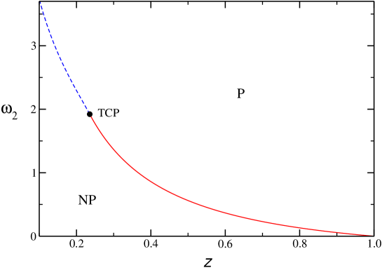
with b=1+2ω2α+ω22α+4ω2+4ω2α+1𝑏12superscriptsubscript𝜔2𝛼superscriptsubscript𝜔22𝛼4subscript𝜔24superscriptsubscript𝜔2𝛼1b=\sqrt{1+2\omega_{2}^{\alpha}+\omega_{2}^{2\alpha}+4\omega_{2}+4\omega_{2}^{\alpha+1}}. Actually, in each approach, there are two of such roots, but one of them leads to inconsistent values of z𝑧z, being ω2θ=1.9217693superscriptsubscript𝜔2𝜃1.9217693\omega_{2}^{\theta}=1.9217693 (A), ω2θ=3.3455816superscriptsubscript𝜔2𝜃3.3455816\omega_{2}^{\theta}=3.3455816 (B) and ω2θ=12.4023526superscriptsubscript𝜔2𝜃12.4023526\omega_{2}^{\theta}=12.4023526 (C) the physical ones. Inserting these values in Eq. 10 one readily finds zθ=0.2355927superscript𝑧𝜃0.2355927z^{\theta}=0.2355927 (A), zθ=0.2083038superscript𝑧𝜃0.2083038z^{\theta}=0.2083038 (B) and zθ=0.1644782superscript𝑧𝜃0.1644782z^{\theta}=0.1644782 (C). In the region z<zθ𝑧superscript𝑧𝜃z<z^{\theta} (where ω2>ω2θsubscript𝜔2superscriptsubscript𝜔2𝜃\omega_{2}>\omega_{2}^{\theta}) both phases coexist. One example of this phase behavior is presented in Fig. 5 for case A and analogous ones are obtained in other approaches (not shown).
Refer to caption
Figure 5: (Color online) Phase diagram for approach A and ω1=0subscript𝜔10\omega_{1}=0. The full (red) and dashed (blue) lines are the critical and coexistence lines, respectively. The black dot indicate the tricritical point.

Although a coil-globule transition is present in this case, the globule phase is different from the one for ω1>0subscript𝜔10\omega_{1}>0, since ω1=0subscript𝜔10\omega_{1}=0 forbids the presence of NN monomers in the system (i.e., ρNN=0subscript𝜌𝑁𝑁0\rho_{NN}=0). For instance, from the expressions for the densities of monomers ρ𝜌\rho and NNN monomers ρNNNsubscript𝜌𝑁𝑁𝑁\rho_{NNN} (not shown explicitly here), it is possible to demonstrate that ρ1𝜌1\rho\rightarrow 1 and ρNNN1subscript𝜌𝑁𝑁𝑁1\rho_{NNN}\rightarrow 1, in the limit ω2subscript𝜔2\omega_{2}\rightarrow\infty, for any approach when ω1>0subscript𝜔10\omega_{1}>0. However, for ω1=0subscript𝜔10\omega_{1}=0, a diverging ω2subscript𝜔2\omega_{2} leads to ρ3/4𝜌34\rho\rightarrow 3/4 and ρNNN7/10subscript𝜌𝑁𝑁𝑁710\rho_{NNN}\rightarrow 7/10 (in case A), ρ3/4𝜌34\rho\rightarrow 3/4 and ρNNN2/3subscript𝜌𝑁𝑁𝑁23\rho_{NNN}\rightarrow 2/3 (in B), and ρ2/3𝜌23\rho\rightarrow 2/3 and ρNNN1/2subscript𝜌𝑁𝑁𝑁12\rho_{NNN}\rightarrow 1/2 (in C), which corresponds to “soft” polymerized phases (and respective “soft globules”), since the maximal occupation of the lattice is smaller than one. In a canonical situation (of polymers with fixed size), this “soft” phase (for ω1=0subscript𝜔10\omega_{1}=0) shall occupy a volume larger than the “regular” globule phase (for ω1>0subscript𝜔10\omega_{1}>0).

We claim that this “soft” globule phase is not a feature of the Husimi lattice, but it might exist also in the square (and other regular) lattices. In fact, although NN monomers are forbidden, the attractive force between NNN monomers that are not part of a bending can acts to collapse the chains, in a similar way as the NN one in the ordinary ISAW model. Moreover, the NNN interaction enhances the formation of bends and, consequently, the formation of globules. Anyhow, more studies are necessary to confirm this.

III.2 Infinite repulsion between NNN monomers (ω2=0subscript𝜔20\omega_{2}=0)

Now, we turn our attention for the case of forbidden NNN monomers. Making ω2=0subscript𝜔20\omega_{2}=0 in the RR’s (Eqs. 6), their solution for the polymerized phase can also be found exactly, being R2=R4=R5=R7=R8=0subscript𝑅2subscript𝑅4subscript𝑅5subscript𝑅7subscript𝑅80R_{2}=R_{4}=R_{5}=R_{7}=R_{8}=0, and R1=a/24+(z+z2/24)/a+z/241/2subscript𝑅1𝑎24𝑧superscript𝑧224𝑎𝑧2412R_{1}=a/24+(z+z^{2}/24)/a+z/24-1/2, with a(36z2+216z+z3+243z3+81z2)1/3𝑎superscript36superscript𝑧2216𝑧superscript𝑧3243superscript𝑧381superscript𝑧213a\equiv\left(36z^{2}+216z+z^{3}+24\sqrt{3z^{3}+81z^{2}}\right)^{1/3}, R3=(1+2R1)/zsubscript𝑅312subscript𝑅1𝑧R_{3}=(1+2R_{1})/z and R6=R1(1+R1)/zsubscript𝑅6subscript𝑅11subscript𝑅1𝑧R_{6}=\sqrt{R_{1}(1+R_{1})/z}, in approaches A and B. In case C, one finds R1=z1/2subscript𝑅1𝑧12R_{1}=z-1/2, R3=1subscript𝑅31R_{3}=1, R6=4z2/2subscript𝑅64𝑧22R_{6}=\sqrt{4z-2}/2 and Ri=0subscript𝑅𝑖0R_{i}=0 otherwise. Noteworthy, this fixed point is independent of ω1subscript𝜔1\omega_{1}, indicating that the thermodynamic properties of the model will not depend on this parameter, as expected.

In approaches A and B, the only non-null eigenvalue of the Jacobian matrix in NP phase is λ=z𝜆𝑧\lambda=z, so, this phase is stable for z1𝑧1z\leq 1 and its spinodal is at z=1𝑧1z=1. The fixed point above for the P phase is physical (and stable) for z1𝑧1z\geq 1 and its stability limit is at z=1𝑧1z=1. Therefore, the phase diagrams in both approaches present only a critical line at z=1𝑧1z=1 separating the NP and P phases, which is consistent with a θ𝜃\theta-point located at zθ=1superscript𝑧𝜃1z^{\theta}=1 and ω1θsuperscriptsubscript𝜔1𝜃\omega_{1}^{\theta}\rightarrow\infty, as already discussed. In case C, we have the same scenario, but the critical line is at z=1/2𝑧12z=1/2.

Notice that ω2=0subscript𝜔20\omega_{2}=0 leads to ρNNN=0subscript𝜌𝑁𝑁𝑁0\rho_{NNN}=0, so that all polymer chains are straight in cases A and B. As already noticed, in case C, the chains are not necessarily straight, since they can bend out the elementary squares and still have ρNNN=0subscript𝜌𝑁𝑁𝑁0\rho_{NNN}=0. In all cases, ρNN=0subscript𝜌𝑁𝑁0\rho_{NN}=0 is also found, as expected, since the infinite repulsion between NNN monomers also forbids NN ones. The density of monomers ρ𝜌\rho is a monotonic increasing function of z𝑧z, being ρ=(2z1)/(4z1)𝜌2𝑧14𝑧1\rho=(2z-1)/(4z-1) in approach C. In the other approaches the expressions are too long to be given here, but one also finds ρ=0𝜌0\rho=0 at z=1𝑧1z=1 and ρ1/2𝜌12\rho\rightarrow 1/2 for z𝑧z\rightarrow\infty. On the square lattice this shall corresponds to a “soft crystalline” phase, where half of the rows (or columns) of the lattice are occupied by straight, parallel and alternating chains. Indeed, placing such aligned (repulsive) polymer chains on a square lattice is analogous to the athermal problem of place infinite rigid rods with NNN exclusion. We remark that athermal lattice gases with exclusion of neighbors have been considered in literature for several ranges of exclusion (or particle sizes) heitor ; nath as well as mixtures of them TiagoGRM . Furthermore, isotropic-nematic transitions in rigid rods is a problem largely studied (see e. g. jurgenLC ; jurgenLC2 for recent surveys). However, for the best of our knowledge, rigid rods with neighbor exclusion has been considered only in the case of dimers with NN exclusion dickman only.

Anyhow, the case of infinite rods with NNN exclusion can be solved on the square lattice, for example, following the recent transfer matrix (TM) calculation by Stilck and Rajesh jurgenLC2 . Considering the limit of infinite rods, without neighbor exclusion, on a roted square lattice yielding a diagonal TM, those authors showed that the (degenerated) spectrum of eigenvalues of the TM is given by Λk=zmsubscriptΛ𝑘superscript𝑧𝑚\Lambda_{k}=z^{m}, with m=0,1,,L𝑚01𝐿m=0,1,\ldots,L or Λk=0subscriptΛ𝑘0\Lambda_{k}=0 jurgenLC2 . This result is for an infinite stripe (in vertical) with width L𝐿L and periodic boundary conditions in horizontal (for more details see jurgenLC2 ). One notices that all rods are parallel in this limiting case and that an eigenvalue of type zmsuperscript𝑧𝑚z^{m} is associated to a state of the system with m𝑚m parallel rods in horizontal direction. So, it is easy to particularize these results for the case with infinite NNN repulsion, by noting that two rods can not occupy adjacent columns (or rows) of the lattice. This will simply reduce the number of states of the TM and, consequently, the spectrum of eigenvalues, which shall be Λk=zmsubscriptΛ𝑘superscript𝑧𝑚\Lambda_{k}=z^{m}, with m=0,1,,L/2𝑚01𝐿2m=0,1,\ldots,L/2 or Λk=0subscriptΛ𝑘0\Lambda_{k}=0, since on a stripe of (even) width L𝐿L it is possible to exist at most L/2𝐿2L/2 parallel rods/chains, due to exclusion. Thence, the largest eigenvalue ΛlsubscriptΛ𝑙\Lambda_{l} and, consequently, the free energy f=1LlnΛl𝑓1𝐿subscriptΛ𝑙f=\frac{1}{L}\ln\Lambda_{l} and the density of monomers ρ=z(fz)𝜌𝑧𝑓𝑧\rho=z\left(\frac{\partial f}{\partial z}\right) are: Λl=1subscriptΛ𝑙1\Lambda_{l}=1, f=0𝑓0f=0 and ρ=0𝜌0\rho=0, for z1𝑧1z\leq 1; and Λl=zL/2subscriptΛ𝑙superscript𝑧𝐿2\Lambda_{l}=z^{L/2}, f=12lnz𝑓12𝑧f=\frac{1}{2}\ln z and ρ=1/2𝜌12\rho=1/2, for z>1𝑧1z>1. Namely, the system undergoes a discontinuous transition at z=1𝑧1z=1 from an empty lattice (the NP phase - for z1𝑧1z\leq 1) to a low density nematic phase (the “soft crystalline” polymer phase - for z>1𝑧1z>1).

Although the Husimi solution yields the correct transition point z=1𝑧1z=1 (at least in the more realistic A and B approaches), the continuous transition found is more a feature of the hierarchical lattice. At first, it is unexpected to find a continuous transition in a mean-field calculation, while the real transition is discontinuous. One recall, notwithstanding, that similar inversions have been observed in other models for θ𝜃\theta-polymers, with discontinuous transitions observed in simulations and continuous ones in exact solutions on hierarchical lattices Tiago ; Tiago2 .

IV Final Discussions and conclusions

In summary, we have studied a generalized ISAW model - where different forces exist between nearest-neighbor (NN) and next-nearest-neighbor (NNN) monomers - on a Husimi lattice built with squares. Three definitions of second neighbors - or interactions between them - have been considered, which effectively overestimate, match or underestimate the number of NNN monomers, compared with square lattice. Since all approaches leads to analogous thermodynamic behaviors, this suggests that a similar scenario can exists also on the regular lattice.
Refer to caption
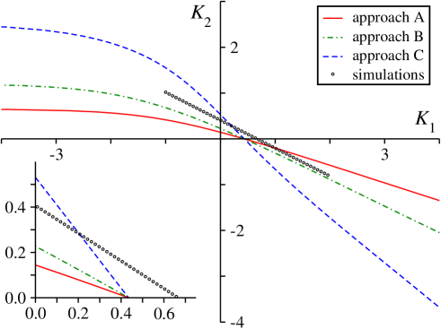
Figure 6: (Color online) Canonical phase diagrams, in variables K2=lnω2subscript𝐾2subscript𝜔2K_{2}=\ln\omega_{2} against K1=lnω1subscript𝐾1subscript𝜔1K_{1}=\ln\omega_{1}, for approaches A (full, blue) and B (dashed, red) and simulational (dash-dotted, black line) results from Ref. Nathann . The inset shows the same data in the region of attractive interactions.

Indeed, our findings are in good agreement with the ones from Monte Carlo simulations on square and cubic lattices Nathann , where only a θ𝜃\theta-line was observed, as well as with previous results from exact enumerations Lee2 . Interestingly, approximately linear θ𝜃\theta-lines were found in the canonical phase diagrams reported in these works, around the region of positive energies. Figure 6 shows the mapping of our grand-canonical phase diagrams in the canonical variables K2ϵ2/kbT(=lnω2)subscript𝐾2annotatedsubscriptitalic-ϵ2subscript𝑘𝑏𝑇absentsubscript𝜔2K_{2}\equiv\epsilon_{2}/k_{b}T(=\ln\omega_{2}) versus K1ϵ1/kbT(=lnω1)subscript𝐾1annotatedsubscriptitalic-ϵ1subscript𝑘𝑏𝑇absentsubscript𝜔1K_{1}\equiv\epsilon_{1}/k_{b}T(=\ln\omega_{1}) and, indeed, almost linear behaviors are found around the first quadrant of the diagrams, but the whole θ𝜃\theta-lines are curved. For comparison, the θ𝜃\theta-line found in simulations of the model on square lattice, K20.6099K1+0.4066similar-to-or-equalssubscript𝐾20.6099subscript𝐾10.4066K_{2}\simeq-0.6099K_{1}+0.4066 Nathann , is also shown in Fig. 6. In the region corresponding to attractive interactions (highlighted in the inset), the θ𝜃\theta-line from approaches A and B are always below the one from simulations, which is expected, since mean-field results generally underestimate the (tri)critical points. A similar behavior is found for small K2subscript𝐾2K_{2} in approach C, but as this parameter increases its θ𝜃\theta-line crosses the one from simulations, which is simply due to the underestimate in the number of NNN sites/monomers in this approach. Linear fits of the θ𝜃\theta-lines in the attractive region return the slopes 0.3330.333-0.333 (in case A), 0.5220.522-0.522 (in B) and 1.2211.221-1.221 (in C), which are approximately 55%, 86% and 200% of the value found in simulations. These behaviors are physically reasonable, because in a collapsing chain each monomer can have at most 2 NN monomers, while in approaches A, B and C it can have effectively a maximum of 6, 4 and 2 NNN monomers, respectively, which is consistent with K2K1/3similar-tosubscript𝐾2subscript𝐾13K_{2}\sim-K_{1}/3 (in A), K2K1/2similar-tosubscript𝐾2subscript𝐾12K_{2}\sim-K_{1}/2 (in B) and K2K1similar-tosubscript𝐾2subscript𝐾1K_{2}\sim-K_{1} (in C).

Acknowledgements.
This work was supported by CNPq and FAPEMIG (brazilian agencies). The author thanks JF Stilck for a critical reading of this manuscript and the kind hospitality of the group of Prof. James Evans at Iowa State University, where part of this work was done.

Appendix A Free Energy

The grand-canonical free energy of the model on the Cayley tree with M𝑀M generations is Φ~M=kBTlnYMsubscript~Φ𝑀subscript𝑘𝐵𝑇subscript𝑌𝑀{\tilde{\Phi}_{M}}=-k_{B}T\ln Y_{M} and one may, conveniently, define the adimensional free energy as ΦM=Φ~M/kBTsubscriptΦ𝑀subscript~Φ𝑀subscript𝑘𝐵𝑇\Phi_{M}={\tilde{\Phi}_{M}}/k_{B}T. Assuming that each surface site has a free energy ϕssubscriptitalic-ϕ𝑠\phi_{s}, while the ones in bulk has ϕbsubscriptitalic-ϕ𝑏\phi_{b} Gujrati , it reads

ΦM=NsMϕs+NbMϕb,subscriptΦ𝑀superscriptsubscript𝑁𝑠𝑀subscriptitalic-ϕ𝑠superscriptsubscript𝑁𝑏𝑀subscriptitalic-ϕ𝑏\Phi_{M}=N_{s}^{M}\phi_{s}+N_{b}^{M}\phi_{b}, (12)

where NsMsuperscriptsubscript𝑁𝑠𝑀N_{s}^{M} and NbMsuperscriptsubscript𝑁𝑏𝑀N_{b}^{M} are the number of sites at surface and bulk, respectively, in generation M𝑀M. Considering a Cayley tree built with squares and ramification σ𝜎\sigma (coordination number q=2(σ+1)𝑞2𝜎1q=2(\sigma+1)), these numbers are

NsM=4(3σ)M1andNbM=4(3σ)M113σ1.formulae-sequencesuperscriptsubscript𝑁𝑠𝑀4superscript3𝜎𝑀1andsuperscriptsubscript𝑁𝑏𝑀4superscript3𝜎𝑀113𝜎1N_{s}^{M}=4(3\sigma)^{M-1}\quad\quad\text{and}\quad\quad N_{b}^{M}=4\dfrac{(3\sigma)^{M-1}-1}{3\sigma-1}. (13)

From these equations, one finds

ϕb=14[ΦM+13σΦM]=14ln[YM+1YM3σ],subscriptitalic-ϕ𝑏14delimited-[]subscriptΦ𝑀13𝜎subscriptΦ𝑀14subscript𝑌𝑀1superscriptsubscript𝑌𝑀3𝜎\phi_{b}=\dfrac{1}{4}\left[\Phi_{M+1}-3\sigma\Phi_{M}\right]=-\dfrac{1}{4}\ln\left[\dfrac{Y_{M+1}}{Y_{M}^{3\sigma}}\right], (14)

which is the reduced free energy in the bulk of the Cayley tree built with squares, i. e., the Husimi lattice.

As discussed in Sec. II, in general, one may write YM=(g0M)4σysubscript𝑌𝑀superscriptsuperscriptsubscript𝑔0𝑀4𝜎𝑦Y_{M}=(g_{0}^{M})^{4\sigma}y and so YM+1=(g0M+1)4σysubscript𝑌𝑀1superscriptsuperscriptsubscript𝑔0𝑀14𝜎𝑦Y_{M+1}=(g_{0}^{M+1})^{4\sigma}y (where y=yA𝑦subscript𝑦𝐴y=y_{A} or y=yB𝑦subscript𝑦𝐵y=y_{B} depending on the approach). In addition, it is easy to see that g0M+1=(g0M)3σR0superscriptsubscript𝑔0𝑀1superscriptsuperscriptsubscript𝑔0𝑀3𝜎subscript𝑅0g_{0}^{M+1}=(g_{0}^{M})^{3\sigma}R_{0}, then

limMYM+1YM3σ=R04σy3σ1,subscript𝑀subscript𝑌𝑀1superscriptsubscript𝑌𝑀3𝜎superscriptsubscript𝑅04𝜎superscript𝑦3𝜎1\lim_{M\to\infty}\frac{Y_{M+1}}{Y_{M}^{3\sigma}}=\frac{R_{0}^{4\sigma}}{y^{3\sigma-1}}, (15)

leading finally to

ϕb=14[4σlnR0(3σ1)lny].subscriptitalic-ϕ𝑏14delimited-[]4𝜎subscript𝑅03𝜎1𝑦\phi_{b}=-\frac{1}{4}[4\sigma\ln R_{0}-(3\sigma-1)\ln y]. (16)

For the case σ=1𝜎1\sigma=1, considered in this work, the expressions for R0subscript𝑅0R_{0} are given in Eq. 6h, while yY/g004𝑦𝑌superscriptsubscript𝑔004y\equiv Y/g_{00}^{4} can be easily calculated from Eq. II, setting α=1𝛼1\alpha=1 (in approach A), α=1/2𝛼12\alpha=1/2 (in B) or α=0𝛼0\alpha=0 (in C).

Appendix B Tricritical lines

At the tricritical condition the solution of the recursion relations (RR’s - Eqs. 6 and 7) must be triply degenerated. Then, one may find the points at the parameter space where this happens, bearing in mind that they shall be on the NP spinodal.

In NP phase Ri=1subscript𝑅𝑖1R_{i}=1 for i=3𝑖3i=3 and Ri=0subscript𝑅𝑖0R_{i}=0 otherwise, so, near the critical surface (and the tricritical line), one may expand the RR’s around, for example, R6subscript𝑅6R_{6} keeping only the terms up to third order. A simple inspection of the RR’s (Eq. 6) shows that RiaiR62similar-to-or-equalssubscript𝑅𝑖subscript𝑎𝑖superscriptsubscript𝑅62R_{i}\simeq a_{i}R_{6}^{2} for i=1,2,4,5𝑖1245i=1,2,4,5 and 888, R31+a3R62similar-to-or-equalssubscript𝑅31subscript𝑎3superscriptsubscript𝑅62R_{3}\simeq 1+a_{3}R_{6}^{2} and R7a7,1R+a7,2R63similar-to-or-equalssubscript𝑅7subscript𝑎71𝑅subscript𝑎72superscriptsubscript𝑅63R_{7}\simeq a_{7,1}R+a_{7,2}R_{6}^{3}. Inserting this in the RR’s and expanding them up to order R63superscriptsubscript𝑅63R_{6}^{3}, one finds

D𝐷\displaystyle D \displaystyle\approx 1+C0R621subscript𝐶0superscriptsubscript𝑅62\displaystyle 1+C_{0}R_{6}^{2} (17a)
Da1R62𝐷subscript𝑎1superscriptsubscript𝑅62\displaystyle Da_{1}R_{6}^{2} \displaystyle\approx C1R62subscript𝐶1superscriptsubscript𝑅62\displaystyle C_{1}R_{6}^{2} (17b)
Da2R62𝐷subscript𝑎2superscriptsubscript𝑅62\displaystyle Da_{2}R_{6}^{2} \displaystyle\approx C2R62subscript𝐶2superscriptsubscript𝑅62\displaystyle C_{2}R_{6}^{2} (17c)
D(1+a3R62)𝐷1subscript𝑎3superscriptsubscript𝑅62\displaystyle D(1+a_{3}R_{6}^{2}) \displaystyle\approx 1+C3R621subscript𝐶3superscriptsubscript𝑅62\displaystyle 1+C_{3}R_{6}^{2} (17d)
Da4R62𝐷subscript𝑎4superscriptsubscript𝑅62\displaystyle Da_{4}R_{6}^{2} \displaystyle\approx C4R62subscript𝐶4superscriptsubscript𝑅62\displaystyle C_{4}R_{6}^{2} (17e)
Da5R62𝐷subscript𝑎5superscriptsubscript𝑅62\displaystyle Da_{5}R_{6}^{2} \displaystyle\approx C5R62subscript𝐶5superscriptsubscript𝑅62\displaystyle C_{5}R_{6}^{2} (17f)
DR6𝐷subscript𝑅6\displaystyle DR_{6} \displaystyle\approx C6,1R6+C6,2R63subscript𝐶61subscript𝑅6subscript𝐶62superscriptsubscript𝑅63\displaystyle C_{6,1}R_{6}+C_{6,2}R_{6}^{3} (17g)
D(a7,1R6+a7,2R63)𝐷subscript𝑎71subscript𝑅6subscript𝑎72superscriptsubscript𝑅63\displaystyle D(a_{7,1}R_{6}+a_{7,2}R_{6}^{3}) \displaystyle\approx C7,1R6+C7,2R63subscript𝐶71subscript𝑅6subscript𝐶72superscriptsubscript𝑅63\displaystyle C_{7,1}R_{6}+C_{7,2}R_{6}^{3} (17h)
Da8R62𝐷subscript𝑎8superscriptsubscript𝑅62\displaystyle Da_{8}R_{6}^{2} \displaystyle\approx C8R62subscript𝐶8superscriptsubscript𝑅62\displaystyle C_{8}R_{6}^{2} (17i)

where

C0subscript𝐶0\displaystyle C_{0} =\displaystyle= 6a1+3a2+za86subscript𝑎13subscript𝑎2𝑧subscript𝑎8\displaystyle 6a_{1}+3a_{2}+za_{8} (18a)
C1subscript𝐶1\displaystyle C_{1} =\displaystyle= za8+z2b2𝑧subscript𝑎8superscript𝑧2superscript𝑏2\displaystyle za_{8}+z^{2}b^{2} (18b)
C2subscript𝐶2\displaystyle C_{2} =\displaystyle= z3ω2b2superscript𝑧3subscript𝜔2superscript𝑏2\displaystyle z^{3}\omega_{2}b^{2} (18c)
C3subscript𝐶3\displaystyle C_{3} =\displaystyle= 2(1+ω2α)a1+2ω2αa2+2a1+a2+zω2a821superscriptsubscript𝜔2𝛼subscript𝑎12superscriptsubscript𝜔2𝛼subscript𝑎22subscript𝑎1subscript𝑎2𝑧subscript𝜔2subscript𝑎8\displaystyle 2(1+\omega_{2}^{\alpha})a_{1}+2\omega_{2}^{\alpha}a_{2}+2a_{1}+a_{2}+z\omega_{2}a_{8} (18d)
C4subscript𝐶4\displaystyle C_{4} =\displaystyle= ω1[zω2αa8+2ω2z2b(ω2α+ω22αa7,1)]subscript𝜔1delimited-[]𝑧superscriptsubscript𝜔2𝛼subscript𝑎82subscript𝜔2superscript𝑧2𝑏superscriptsubscript𝜔2𝛼superscriptsubscript𝜔22𝛼subscript𝑎71\displaystyle\omega_{1}[z\omega_{2}^{\alpha}a_{8}+2\omega_{2}z^{2}b(\omega_{2}^{\alpha}+\omega_{2}^{2\alpha}a_{7,1})] (18e)
C5subscript𝐶5\displaystyle C_{5} =\displaystyle= 4ω12ω22z3(ω2α+ω22αa7,1)24superscriptsubscript𝜔12superscriptsubscript𝜔22superscript𝑧3superscriptsuperscriptsubscript𝜔2𝛼superscriptsubscript𝜔22𝛼subscript𝑎712\displaystyle 4\omega_{1}^{2}\omega_{2}^{2}z^{3}(\omega_{2}^{\alpha}+\omega_{2}^{2\alpha}a_{7,1})^{2} (18f)
C6,1subscript𝐶61\displaystyle C_{6,1} =\displaystyle= zb+ω2z2b𝑧𝑏subscript𝜔2superscript𝑧2𝑏\displaystyle zb+\omega_{2}z^{2}b (18g)
C6.2subscript𝐶6.2\displaystyle C_{6.2} =\displaystyle= ω2z2b(a3+2ω2αa4+ω22αa5)+2ω2α+1z2a7,2+ω2(2ω2αa1+ω22αa2)z2bsubscript𝜔2superscript𝑧2𝑏subscript𝑎32superscriptsubscript𝜔2𝛼subscript𝑎4superscriptsubscript𝜔22𝛼subscript𝑎52superscriptsubscript𝜔2𝛼1superscript𝑧2subscript𝑎72subscript𝜔22superscriptsubscript𝜔2𝛼subscript𝑎1superscriptsubscript𝜔22𝛼subscript𝑎2superscript𝑧2𝑏\displaystyle\omega_{2}z^{2}b(a_{3}+2\omega_{2}^{\alpha}a_{4}+\omega_{2}^{2\alpha}a_{5})+2\omega_{2}^{\alpha+1}z^{2}a_{7,2}+\omega_{2}(2\omega_{2}^{\alpha}a_{1}+\omega_{2}^{2\alpha}a_{2})z^{2}b
+\displaystyle+ 2ω1z2ω2α+1a8(ω2α+ω22αa7,1)+2zω2αa7,2+[(2(1+ω2α))a1+2ω2αa2]zb2subscript𝜔1superscript𝑧2superscriptsubscript𝜔2𝛼1subscript𝑎8superscriptsubscript𝜔2𝛼superscriptsubscript𝜔22𝛼subscript𝑎712𝑧superscriptsubscript𝜔2𝛼subscript𝑎72delimited-[]21superscriptsubscript𝜔2𝛼subscript𝑎12superscriptsubscript𝜔2𝛼subscript𝑎2𝑧𝑏\displaystyle 2\omega_{1}z^{2}\omega_{2}^{\alpha+1}a_{8}(\omega_{2}^{\alpha}+\omega_{2}^{2\alpha}a_{7,1})+2z\omega_{2}^{\alpha}a_{7,2}+[(2(1+\omega_{2}^{\alpha}))a_{1}+2\omega_{2}^{\alpha}a_{2}]zb
C7,1subscript𝐶71\displaystyle C_{7,1} =\displaystyle= 2ω1ω22z3(ω2α+ω22αa7,1)2subscript𝜔1superscriptsubscript𝜔22superscript𝑧3superscriptsubscript𝜔2𝛼superscriptsubscript𝜔22𝛼subscript𝑎71\displaystyle 2\omega_{1}\omega_{2}^{2}z^{3}(\omega_{2}^{\alpha}+\omega_{2}^{2\alpha}a_{7,1}) (18i)
C7,2subscript𝐶72\displaystyle C_{7,2} =\displaystyle= ω1ω2[ω2αz2a8b+2ω2z3(ω2α+ω22αa7,1)(2a3+4ω2αa4+2ω22αa5)+2ω22α+1z3a7,2\displaystyle\omega_{1}\omega_{2}[\omega_{2}^{\alpha}z^{2}a_{8}b+2\omega_{2}z^{3}(\omega_{2}^{\alpha}+\omega_{2}^{2\alpha}a_{7,1})(2a_{3}+4\omega_{2}^{\alpha}a_{4}+2\omega_{2}^{2\alpha}a_{5})+2\omega_{2}^{2\alpha+1}z^{3}a_{7,2}
+\displaystyle+ ω1ω2(8z3(ω2α+ω22αa7,1)3+2z3ω22αa8(ω2α+ω22αa7,1))]\displaystyle\omega_{1}\omega_{2}(8z^{3}(\omega_{2}^{\alpha}+\omega_{2}^{2\alpha}a_{7,1})^{3}+2z^{3}\omega_{2}^{2\alpha}a_{8}(\omega_{2}^{\alpha}+\omega_{2}^{2\alpha}a_{7,1}))]
C8subscript𝐶8\displaystyle C_{8} =\displaystyle= ω2[z2b2+8ω1z3ω2(ω2α+ω22αa7,1)2]subscript𝜔2delimited-[]superscript𝑧2superscript𝑏28subscript𝜔1superscript𝑧3subscript𝜔2superscriptsuperscriptsubscript𝜔2𝛼superscriptsubscript𝜔22𝛼subscript𝑎712\displaystyle\omega_{2}[z^{2}b^{2}+8\omega_{1}z^{3}\omega_{2}(\omega_{2}^{\alpha}+\omega_{2}^{2\alpha}a_{7,1})^{2}] (18k)

with b1+ω2α+2ω2αa7,1𝑏1superscriptsubscript𝜔2𝛼2superscriptsubscript𝜔2𝛼subscript𝑎71b\equiv 1+\omega_{2}^{\alpha}+2\omega_{2}^{\alpha}a_{7,1} and α=1𝛼1\alpha=1 (in case A), α=1/2𝛼12\alpha=1/2 (in B) or α=0𝛼0\alpha=0 (in C).

Equating the terms of same order in Eqs. (17a)-(17i), the relations ai=Cisubscript𝑎𝑖subscript𝐶𝑖a_{i}=C_{i} for i=1,2,4,5,8𝑖12458i=1,2,4,5,8 and a3+C0=C3subscript𝑎3subscript𝐶0subscript𝐶3a_{3}+C_{0}=C_{3}, a7,1=C7,1subscript𝑎71subscript𝐶71a_{7,1}=C_{7,1} and a7,2+a7,1C0=C7,2subscript𝑎72subscript𝑎71subscript𝐶0subscript𝐶72a_{7,2}+a_{7,1}C_{0}=C_{7,2} are obtained, allowing us to determine all aisubscript𝑎𝑖a_{i}’s as functions of z𝑧z, ω1subscript𝜔1\omega_{1} and ω2subscript𝜔2\omega_{2}. Using these functions in the two additional equations C6,1=1subscript𝐶611C_{6,1}=1 - which leads to the same expression for the stability limit of the NP phase (Eq. 8) - and C6,2=C0subscript𝐶62subscript𝐶0C_{6,2}=C_{0}, the tricritical line is found. Although we do not find a closed expression for this line, it can be easily calculated with the help of an algebra software.

References

  • (1) P. G. de Gennes, J. Phys. (Paris), Lett. 36 L55 (1975).
  • (2) P. G. de Gennes, Scaling Concepts in Polymer Physics (Cornell Univ. Press, Ithaca, NY, 1979).
  • (3) P. J. Flory, J. Chem. Phys. 17, 303 (1949).
  • (4) P. J. Flory, Principles of Polymer Chemistry (Cornell Univ. Press, Ithaca, NY, 1966).
  • (5) C. Vanderzande, Lattice models of polymers (Cambridge Univ. Press, Cambridge, UK, 1998).
  • (6) B. Duplantier, and H. Saleur, Phys. Rev. Lett. 59, 539 (1987); ibid 60, 1204 (1988); ibid 62, 1368 (1989).
  • (7) E. Botelho, and J. F. Stilck, Phys. Rev. E 48, 723 (1993).
  • (8) S. Lise, A. Maritan, and A. Pelizzola, Phys. Rev. E 58 R5241 (1998).
  • (9) M. Pretti, Phys. Rev. E 66, 061802 (2002).
  • (10) Jie Zhou, Zhong-Can Ou-Yang, and Haijun Zhou, J. Chem. Phys. 128, 124905 (2008).
  • (11) J. H. Lee, S.-Y. Kim, and J. Lee, J. Chem. Phys. 135, 204102 (2011).
  • (12) J. H. Lee, S.-Y. Kim, and J. Lee, Phys. Rev. E 87, 052601 (2013)
  • (13) N. T. Rodrigues, and T. J. Oliveira, J. Phys. A 47, 405002 (2014).
  • (14) S. Jin, A. Sen, W. Guo, and A. W. Sandvik, Phys. Rev. B 87, 144406 (2013).
  • (15) J. Krawczyk, T. Prellberg, A. L. Owczarek, and A. Rechnitzer, Phys. Rev. Lett. 96, 240603 (2006).
  • (16) T. J. Oliveira, J. F. Stilck, and P. Serra, Phys. Rev. E 80, 041804 (2009); T. J. Oliveira and J. F. Stilck, J. Stat. Mech. 2011, P01026 (2011).
  • (17) R. J. Baxter, Exactly Solved Models in Statistical Mechanics, Academic, London (1982).
  • (18) P. D. Gujrati, Phys. Rev. Lett. 74, 809 (1995).
  • (19) H. C. M. Fernandes, J. J. Arenzon, and Y. Levin, J. Chem. Phys. 126, 114508 (2007), and references therein.
  • (20) T. Nath and R. Rajesh, Phys. Rev. E 90, 012120 (2014), and references therein.
  • (21) T. J. Oliveira, and J. F. Stilck, J. Chem. Phys. 135, 184502 (2011); Phys. Rev. E 92, 032101 (2015).
  • (22) J. Kundu, R. Rajesh, D. Dhar, and J. F. Stilck, Phys. Rev. E 87, 032103 (2013).
  • (23) R. Dickman, J. Chem. Phys. 136, 174105 (2012).
  • (24) J. F. Stilck, and R. Rajesh, Phys. Rev. E 91, 012106 (2015).
  • (25) T. J. Oliveira, and J. F. Stilck, arXiv:1510.07360.