Newtonian kinematical backreaction in cosmological
-body simulations with Delaunay Tesselation:
“zero test” and scale dependence
Abstract
The backreaction of inhomogeneities describes the effect of inhomogeneous structure on average properties of the Universe. We investigate this approach by testing the consistency of cosmological -body simulations as non-linear structure evolves. Using the Delaunay Tessellation Field Estimator (DTFE), we calculate the kinematical backreaction from simulations on different scales in order to measure how much -body simulations should be corrected for this effect. This is the first step towards creating fully relativistic and inhomogeneous -body simulations. In this paper we compare the interpolation techniques available in DTFE and illustrate the statistical dependence of as a function of length scale.
keywords:
large–scale structure, statistics, N-body simulations, interpolation techniques1 Introduction
Inhomogeneous structure of the Universe at scales below is an undeniable fact. The standard approach to model it (i.e., in the standard CDM model approach) is to perturb the homogeneous solution of the Einstein equations, i.e. the Friedmann–Lemaítre–Robertson–Walker (FLRW) metric. However, there are strong suggestions that this approach may not be the best one especially for the late times (i.e. small redshifts ) of the Universe evolution (e.g., Ref. \refcitedeLappGH86).
Another approach, scalar averaging using general relativity (GR), introduces kinematical and curvature backreaction of the inhomogeneous structure of the Universe, in principle without assuming a homogeneous background. Here we focus only on the Newtonian version of this approach [2, 3] since current -body simulations are Newtonian (within the expanding FLRW background, which is rigid in comoving coordinates). Our motivation is to investigate whether the effect, namely kinematical backreaction , described in Ref. \refciteBKS00, exists in -body simulations as the model predicts, and check how big this effect is compared to that expected analytically.
2 Method
In the Newtonian approach there is only the kinematical backreaction111Curvature backreaction is obviously zero because of the flat Euclidean spatial section. which occurs in the generalised acceleration law:[3, 2]
| (1) |
where
| (2) |
The volume-weighted average is defined as a volume integral normalised by the volume of the domain for which averaging is performed. The quantities , and are respectively the expansion rate and the rates of vorticity and shear, defined in the standard way as elements of the decomposition of the velocity gradient tensor in three parts: the trace , the symmetric part and the antisymmetric part . Equation 2 can be rewritten in terms of the tensor invariants:
| (3) |
where
| (4a) | ||||
| (4b) | ||||
and .
2.1 Interpolating and averaging fields from -body simulations
In order to calculate from -body simulations for a given domain one needs to interpolate the velocity field (and its gradient) from a discrete set of points, since in -body simulations all information about fields is encoded in particles. There are several methods for interpolating fields from a set of points (e.g. SPH, CIC). We chose the Delaunay Tessellation Field Estimator222 The code is free-licensed and available at: http://www.astro.rug.nl/~voronoi/DTFE/dtfe.html. DTFE uses CGAL—the Computational Geometry Algorithms Library, also free-licensed (http://www.cgal.org/). (DTFE) [4] method, which is based on Delaunay Triangulation (DT).[5] The advantage of this choice is that it interpolates the velocity field and its gradients in a very natural way, i.e. by linear interpolation inside every Delaunay cell (a tetrahedron in the 3D case).[6] Cells are constructed from a discrete set of points (particles) in such a way that every tetrahedron constructed from 4 particles fulfills the requirement that there is no other particle inside a sphere circumscribed on that tetrahedron.
2.2 “” test for periodic boundary condition
From (2) and (1) it is clear that the backreaction in the Newtonian approach is purely of a kinematical origin. Moreover, because of the way in which it is defined, it will always be zero if there is no boundary, e.g. if the “boundaries” are periodically identified, as is the case for cosmological numerical simulations.333The problem of boundaries in cosmological simulations is “solved” by setting up a topology of the simulation box, i.e. periodic translation of the fields through the opposite faces of the simulation box.. This is due to the fact that, by using Gauss’ theorem, in comoving coordinates can be expressed as an integral over the surface (see eq. (10) of [2]). This gives the possibility to test existing simulations for consistency if they preserve ( denotes the whole simulation domain with topology, “periodic boundary conditions”). If one divides the whole simulation box domain onto smaller cubes (or domains of another shape) of equal volume , then the following equation will be valid:
| (5) |
for .
3 Results
For calculations we used Einstein–de Sitter () -body simulations: (i) a Virgo Consortium (VC) simulation from [7] (simulation SCDM1, hereafter VC EdS) and (ii) our own simulation performed with Gadget-2 (hereafter, Gadget-2 EdS) with the same box size and number of particles and cosmological parameters as in VC EdS (simulation box size: , particles, ).
We tested vanishing with periodic boundary conditions (the “” test) with . For any , this sets up the grid resolution which corresponds to sub-box domains of a fixed size (); and probes all ranges of scales from to for a simulation with a box side length . The velocity gradient was calculated using DTFE with the default volume averaging method, i.e. Monte Carlo sampling over DT cells with approximately 100 samples444The number of samples depends on the ratio between the DT cell volume and the chosen grid cell volume. per each grid cell for a given estimate.
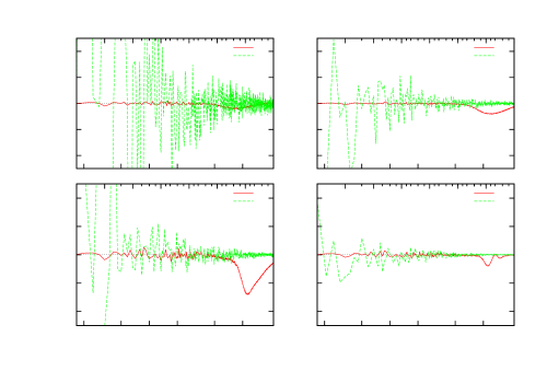
Figure 1 shows as a function of the size of sub-domains (eq. 5), or equivalently, as a function of .
does not stay close to zero for every , particularly for ranging from 128 to 512, where is negative for both the VC EdS and Gadget-2 EdS simulations (top panels of fig.1). This corresponds to . Moreover fig. 1 shows (middle panels) and (bottom panels) from which—with respect to the — was calculated. It is clear that negative values of comes from . Equation (4b) shows that this significant deviation from zero values comes either from overestimation of or underestimation of and/or , since the square of the former provides a negative contribution and square of the latter two positive input to (see eq. 4b).
For a regular grid such as the one used here, DTFE has two built-in methods of interpolating fields to a grid location followed by a local averaging procedure (hereafter, “averaged interpolation”): (i) sampling randomly over Delaunay cells (hereafter, the DT method; as in fig. 1); or (ii) sampling (randomly or not) within the grid cell (hereafter, the grid method). We have performed the same test for both averaged interpolation methods, and varied the numbers of random samples.
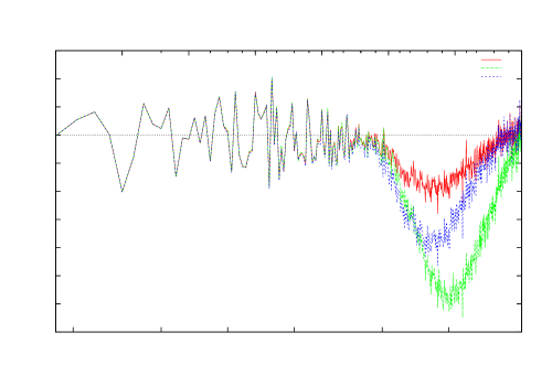
Figure 2 compares these two methods for the “” test with the VC EdS simulation.

The DT method (solid red line) is less noisy in general, but produces strong negative values for . Grid sampling (dashed green line) is more noisy (especially for high ) but does not produce this feature for , even though the sample size per grid cell (by default, 20 random samples) is lower than for the DT method. When is high, the number of particles per grid cell is low, so that Delaunay cells will be large compared to a grid cell; thus, a systematic error in volume-weighted averaging of the velocity gradient could occur by sampling within the local Delaunay cells rather than within the grid cell. This may explain the DT-method high- negative values, in which case increasing the sample size should weaken the negative —figure 4 supports this.
3.1 Statistics of —early results
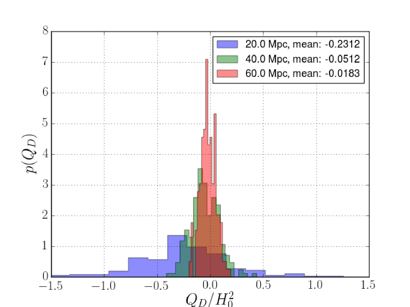
Motivated by the analysis, the DT method, with random sample size increased to 300 and grid size , was used to estimate probability density functions (PDF) of for the VC EdS simulation at redshift . Figure 4 shows PDFs for three different domain sizes, ; in each case, 200 domains were chosen randomly. There is clear evidence of statistical scale dependence for : the smaller the domain , the more negative tends to be (fig. 4). More detailed calculations will be published soon.


4 Summary
Using DTFE to perform the “ test” for the VC EdS and Gadget-2 EdS simulations suggests that the DT method (sampling over DT cells) introduces artificial behaviour for small grid cells, i.e. when the number of grid cells is comparable to the number of particles in simulation. At early epochs, the magnitude of the effect is comparable to that of the noise of the grid-sampling averaged interpolation method for big grid cells (low numbers of grid cells). This systematic error can be reduced by increasing the number of random samples used for averaged interpolations within Delaunay tetrahedra (fig. 4), at the cost of slowing the calculation. The code could be improved by implementing an exact calculation of volume-weighted averages in each grid cell (i.e. averaging the interpolation without random sampling). The PDFs of show statistical scale dependence (fig. 4).
Acknowledgments
TK thanks the National Science Centre, Poland for partial support from an ETIUDA-2 grant as well as to J.J. Ostrowski, B.F. Roukema and T. Buchert for useful comments. Some of this work was done under the National Science Centre, Poland grant 2014/13/B/ST9/00845.
References
- [1] V. de Lapparent, M. J. Geller and J. P. Huchra, A slice of the universe, ApJ 302, L1 (March 1986).
- [2] T. Buchert, M. Kerscher and C. Sicka, Back reaction of inhomogeneities on the expansion: The evolution of cosmological parameters, Phys. Rev. D 62, p. 043525 (August 2000), arXiv:astro-ph/9912347.
- [3] T. Buchert and J. Ehlers, Averaging inhomogeneous Newtonian cosmologies., A&A 320, 1 (April 1997).
- [4] W. E. Schaap and R. van de Weygaert, Continuous fields and discrete samples: reconstruction through Delaunay tessellations, A&A 363, L29 (November 2000), arXiv:astro-ph/0011007.
- [5] B. Delaunay, Sur la sphère vide. A la mémoire de Georges Voronoï, Bull. Acad. Sci. URSS: Classe sci. math. et nat. 6, 739 (1934), http://mi.mathnet.ru/eng/izv4937.
- [6] F. Bernardeau and R. van de Weygaert, A new method for accurate estimation of velocity field statistics, MNRAS 279, p. 693 (March 1996).
- [7] A. Jenkins, C. S. Frenk, F. R. Pearce, P. A. Thomas, J. M. Colberg, S. D. M. White, H. M. P. Couchman, J. A. Peacock, G. Efstathiou and A. H. Nelson, Evolution of Structure in Cold Dark Matter Universes, ApJ 499, p. 20 (May 1998), arXiv:astro-ph/9709010.