Depletion-Induced Forces and Crowding in Polymer-Nanoparticle Mixtures:
Role of Polymer Shape Fluctuations and Penetrability

Abstract

Depletion forces and macromolecular crowding govern the structure and function of biopolymers in biological cells and the properties of polymer nanocomposite materials. To isolate and analyze the influence of polymer shape fluctuations and penetrability on depletion-induced interactions and crowding by nanoparticles, we model polymers as effective penetrable ellipsoids, whose shapes fluctuate according to the probability distributions of the eigenvalues of the gyration tensor of an ideal random walk. Within this model, we apply Monte Carlo simulation methods to compute the depletion-induced potential of mean force between hard nanospheres and crowding-induced shape distributions of polymers in the protein limit, in which polymer coils can be easily penetrated by smaller nanospheres. By comparing depletion potentials from simulations of ellipsoidal and spherical polymer models with predictions of polymer field theory and free-volume theory, we show that polymer depletion-induced interactions and crowding depend sensitively on polymer shapes and penetrability, with important implications for bulk thermodynamic phase behavior.

I Introduction

Depletion forces can profoundly influence the properties of soft materials, e.g., colloid-polymer mixtures Lekkerkerker and Tuinier (2011) and polymer nanocomposites Balazs et al. (2006); Mackay et al. (2006), whose multiple species intermingle and exclude volume to one another. The exclusion of polymers, or other flexible macromolecules, from a layer surrounding rigid colloidal particles creates an imbalance in osmotic pressure that can induce an effective interparticle pair attraction. This depletion mechanism, recognized by Asakura and Oosawa over 60 years ago Asakura and Oosawa (1954), is physically reasonable and well established in the “colloid limit”, in which the particle radius exceeds the average polymer radius of gyration. In the opposite “protein limit”, in which nanoparticles (e.g., globular proteins) can penetrate much larger polymer coils, the concept of a depletion layer around a particle must be replaced by that of a segment-segment correlation length (blob radius) of the polymer coil de Gennes (1979).

Depending on the relative strengths of competing intermolecular interactions Israelachvili (1992), including steric, electrostatic, and van der Waals interactions, depletion-induced attraction can drive aggregation and thermodynamic phase separation, leading, for example, to coexistence of polymer-rich and polymer-poor bulk phases Vrij (1976); Pusey (1991); Jones (2002); Fuchs and Schweizer (2002); Fleer and Tuinier (2008). In soft materials, where effective interactions Denton (2007) between macromolecules are typically comparable in magnitude to thermal energies, and self-assembly often depends on a delicate balance between energy and entropy, depletion can crucially affect phase stability. The ability to control depletion forces has great practical value for stabilizing foods Tolstoguzov (1991); de Kruif and Tuinier (2001) and pharmaceuticals against coagulation, purifying water by flocculation and sedimentation of colloidal particles Norde (2011), guiding the self-assembly of virus particles Dogic et al. (2004); Li et al. (2013), and promoting or inhibiting aggregation of proteins Kulkarni and Zukoski (2001), with relevance for deciphering protein structure via scattering measurements on crystalline samples and treating diseases, such as cataracts Stradner et al. (2007).

An intrinsic complement to depletion is the phenomenon of macromolecular crowding, in which polymers, or other flexible macromolecules, deform in both size and shape in response to confinement by other species or bounding surfaces Minton (1981, 2000, 2001); Richter et al. (2007, 2008); Elcock (2010); Hancock (2012). Kuhn’s prescient insight Kuhn (1934) that a polymer coil in solution fluctuates in shape, being well-approximated by an elongated, flattened ellipsoid (in its principal-axis frame of reference), has inspired numerous mathematical and statistical mechanical analyses of the shapes of random walks Fixman (1962); Flory and Fisk (1966); Flory (1969); Yamakawa (1970); Fujita and Norisuye (1970); Šolc (1971, 1973); Theodorou and Suter (1985); Rudnick and Gaspari (1986, 1987); Bishop and Saltiel (1988); Sciutto (1996); Schäfer (1999); Murat and Kremer (1998); Eurich and Maass (2001). In biology, conformational changes of biopolymers, such as RNA, DNA, and unfolded proteins are important for cellular processes in the crowded environment of the nucleus Ellis (2001a, b); van der Maarel (2008); Phillips et al. (2009); Cheung (2013); Denton (2013), packaging of DNA in viral capsids Ali et al. (2006), and translocation of biopolymers through narrow pores Polson et al. (2013).

Depletion forces, polymer crowding, and phase behavior in colloid-polymer mixtures and polymer-nanoparticle composite materials have been probed by a diverse array of experimental methods, including neutron scattering Ye et al. (1996); Nakatani et al. (2001); Kramer et al. (2005a, b, c); Le Coeur et al. (2009, 2010); Nusser et al. (2010), atomic force microscopy Milling and Biggs (1995), total internal reflection microscopy Rudhardt et al. (1998), optical trapping Verma et al. (1998); Lin et al. (2001); Hilitski et al. (2015), and turbidity measurements Hennequin et al. (2005); Zhang and van Duijneveldt (2006); Mutch et al. (2007). Related modeling approaches have been based on mean-field and scaling theories de Gennes (1979); Joanny et al. (1979); Sear (1997, 2001, 2002), free-volume theories Minton (2005); Denton and Schmidt (2002); Lu and Denton (2011); Lim and Denton (2014), force-balance theory Walz and Sharma (1994), perturbation theory Mao et al. (1995, 1997), polymer field theory Eisenriegler et al. (1996); Hanke et al. (1999); Eisenriegler et al. (2003); Odijk (2000); Woodward and Forsman (2010, 2012); Wang et al. (2014), integral-equation theory Chatterjee and Schweizer (1998); Ramakrishnan et al. (2002); Moncho-Jordá et al. (2003), density-functional theory Bechinger et al. (1999); Schmidt and Fuchs (2002); Goel et al. (2004); Woodward and Forsman (2008); Forsman and Woodward (2009), adsorption theory Tuinier et al. (2000); Tuinier and Lekkerkerker (2001); Tuinier and Petukhov (2002), and simulation of both molecular Meijer and Frenkel (1991, 1994); Dickman and Yethiraj (1994); Bolhuis et al. (2002); Louis et al. (2002); Bolhuis et al. (2003); Doxastakis et al. (2004, 2005); Goldenberg (2003); Dima and Thirumalai (2004); Cheung et al. (2005); Denesyuk and Thirumalai (2011, 2013a); Camargo and Likos (2010); Linhananta et al. (2012); Chen et al. (2012); Cheung (2013) and coarse-grained Hoppe and Yuan (2011); Denesyuk and Thirumalai (2013b); Lu and Denton (2011); Lim and Denton (2014) polymer models.

Previous studies have explored the nature of depletion interactions induced by aspherical depletants of fixed size and shape Mao et al. (1997); Triantafillou and Kamien (1999); Piech and Walz (2000); Lin et al. (2001) and the impact of crowding on polymer size Kramer et al. (2005a, b, c); Le Coeur et al. (2009, 2010); Nusser et al. (2010); Minton (2005); Goldenberg (2003); Dima and Thirumalai (2004); Cheung et al. (2005); Denesyuk and Thirumalai (2011, 2013a). In recent work, we reported on preliminary studies of polymer crowding in models of polymer-nanoparticle mixtures with polymers modeled as fluctuating, penetrable spheres Lu and Denton (2011) or ellipsoids Lim and Denton (2014). In this paper, using a refined model of polymer-nanoparticle penetration, we directly analyze the complex relationships between polymer depletion-induced interactions, nanoparticle crowding, and polymer shape fluctuations. By comparing results with theoretical predictions, we validate the polymer model and demonstrate the significance of shape fluctuations in depletion and crowding phenomena. Our model and computational methods are sufficiently general as to be easily adapted and applied to other soft materials.

The remainder of the paper is assembled as follows. In Sec. II, we review the model of polymers as fluctuating penetrable ellipsoids and the field theory model for the free energy cost of penetrating a polymer by a hard nanosphere. In Sec. III, we outline our simulation methods for computing polymer depletion-induced interactions between nanospheres and crowding-induced deformations in polymer shape. Numerical results are presented in Sec. III and compared with predictions of field theories and free-volume theory. Finally, in Sec. III, we conclude with suggestions for future work.

II Models

II.1 Ellipsoidal Polymer Model

Figure 1: Model of a polymer-nanoparticle mixture with polymers represented as ellipsoids that can fluctuate in size and shape. Nanoparticles are hard spheres of fixed size that are mutually impenetrable, but able to penetrate the polymers. Penetration is defined as the intersection of the surfaces of an ellipsoid and a sphere. For example, the dark nanosphere is just on the verge of penetrating a polymer.

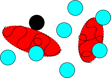
Our model extends the classic Asakura-Oosawa-Vrij (AOV) model of colloid-polymer mixtures Asakura and Oosawa (1954); Vrij (1976). The AOV model represents nonadsorbing polymer coils, in a coarse-grained approximation, as effective spheres of fixed size that are mutually noninteracting, but impenetrable to the colloidal particles. The spherical polymer approximation ignores fluctuations in conformation, while the impenetrable polymer assumption is justified only in the colloid limit, where the polymers are smaller than the particles. As in our previous studies Lim and Denton (2014, 2015), we refine the AOV model by representing the polymers as soft ellipsoids that fluctuate in size and shape and that can be penetrated by smaller nanoparticles.

For simplicity, we focus on linear homopolymers, although the analysis can be generalized to other polymer architectures, such as block copolymers Eurich et al. (2007). A coil of $N$ identical, connected segments has a size and shape characterized by the gyration tensor ${\bf T}$ with components

$$T_{ij}=\frac{1}{N}\sum_{k=1}^{N}r_{ki}r_{kj}~{},$$ (1)

where $r_{ki}$ is $i^{\rm th}$ component of the position vector ${\bf r}_{k}$ of the $k^{\rm th}$ segment relative to the center of mass. The familiar moment of inertia tensor ${\bf I}$ of rigid body dynamics relates to the gyration tensor via ${\bf I}=R_{p}^{2}{\bf 1}-{\bf T}$, where ${\bf 1}$ is the unit tensor and

$$R_{p}=\left(\frac{1}{N}\sum_{i=1}^{N}r_{i}^{2}\right)^{1/2}=(\Lambda_{1}+\Lambda_{2}+\Lambda_{3})^{1/2}$$ (2)

is the radius of gyration of a given conformation of the coil expressed in terms of the eigenvalues $\Lambda_{i}$ ($i=1,2,3$ in three dimensions) of ${\bf T}$. The experimentally measurable root-mean-square (rms) radius of gyration is given by

$$R_{g}=\sqrt{\left\langle R_{p}^{2}\right\rangle}=\sqrt{\left\langle\Lambda_{1}+\Lambda_{2}+\Lambda_{3}\right\rangle}~{},$$ (3)

where the angular brackets represent an ensemble average over polymer conformations.

If the ensemble average in Eq. (3) is evaluated in a reference frame tied to the principal axes of the coil, and the coordinate axes are labelled to preserve the order of the eigenvalues by magnitude ($\Lambda_{1}>\Lambda_{2}>\Lambda_{3}$), then the average tensor is asymmetric and describes an anisotropic object Rudnick and Gaspari (1986, 1987). Averaging in a fixed (laboratory) frame yields, in contrast, a symmetric average tensor that has equal eigenvalues and thus describes a sphere. Simply stated, a fluctuating random walk has an average shape that is spherical when viewed from the laboratory frame, but significantly aspherical – elongated, flattened, bean-shaped – when viewed from the principal-axis frame Kuhn (1934); Šolc (1971, 1973). The general ellipsoid that best fits the shape of the polymer coil – roughly corresponding to the tertiary structure of a biopolymer – has principal radii proportional to the square-roots of the respective eigenvalues of the gyration tensor. In Cartesian $(x,y,z)$ coordinates, the surface is described by

$$\frac{x^{2}}{\Lambda_{1}}+\frac{y^{2}}{\Lambda_{2}}+\frac{z^{2}}{\Lambda_{3}}=3~{}.$$ (4)

The probability distribution for the shape of a freely-jointed polymer coil of $N$ segments of length $l$, modeled as a soft ellipsoid Murat and Kremer (1998), is accurately approximated by the analytical form Eurich and Maass (2001)

$$P_{0}(\lambda_{1},\lambda_{2},\lambda_{3})=P_{1}(\lambda_{1})P_{2}(\lambda_{2})P_{3}(\lambda_{3})~{},$$ (5)

where $\lambda_{i}\equiv\Lambda_{i}/(Nl^{2})$ are scaled (dimensionless) eigenvalues and

$$P_{i}(\lambda_{i})=\frac{(a_{i}d_{i})^{n_{i}-1}\lambda_{i}^{-n_{i}}}{2K_{i}}\exp\left(-\frac{\lambda_{i}}{a_{i}}-d_{i}^{2}\frac{a_{i}}{\lambda_{i}}\right)~{},$$ (6)

with fitting parameters $K_{1}=0.094551$, $K_{2}=0.0144146$, $K_{3}=0.0052767$, $a_{1}=0.08065$, $a_{2}=0.01813$, $a_{3}=0.006031$, $d_{1}=1.096$, $d_{2}=1.998$, $d_{3}=2.684$, $n_{1}=1/2$, $n_{2}=5/2$, and $n_{3}=4$. Although the factorization ansatz of Eq. (5) is not exact, since extensions of a random walk in orthogonal directions are not independent, conformations that seriously violate the ansatz are rare for sufficiently long random walks. It is important to note that the eigenvalue distributions [Eq. (6)] are derived from random-walk segment statistics Murat and Kremer (1998); Eurich and Maass (2001), reflect considerable fluctuations in size and shape of a free polymer, and will be modified by confinement, e.g., for polymers in the presence of nanoparticle crowders.

II.2 Polymer-Nanoparticle Mixtures

A mixture of hard nanospheres and nonadsorbing polymers is characterized by the number densities of the two species, $n_{n}$ and $n_{p}$, the nanosphere radius $R_{n}$, and the rms radius of gyration $R_{g}$ of free (uncrowded) polymer. In the colloid limit ($R_{g}<R_{n}$), in which the polymer coils are impenetrable to particles, the effective polymer size must be calibrated in order to consistently and accurately account for the polymer excluded volume Lim and Denton (2015). In the protein limit ($R_{g}\gg R_{n}$), in which polymer penetration supplants excluded volume, it is instead the penetration energy that must be calibrated, as explained below (Sec. II.3). Thus, we simply take the polymer radius equal to $R_{g}$ and define the polymer-to-nanosphere size ratio as $q\equiv R_{g}/R_{n}$. The volume fractions of the two species are $\phi_{n}\equiv(4\pi/3)n_{n}R_{n}^{3}$ and $\phi_{p}\equiv(4\pi/3)n_{p}R_{g}^{3}$. It should be noted that the actual fraction of volume occupied by polymer coils will differ from $\phi_{p}$ due to the aspherical shapes and interpenetration of the coils.

In terms of the scaled eigenvalues, deviations of a polymer’s average shape from spherical can be quantified by an asphericity parameter Rudnick and Gaspari (1986, 1987)

$$A(\phi_{n})=1-3\frac{\left\langle\lambda_{1}\lambda_{2}+\lambda_{1}\lambda_{3}+\lambda_{2}\lambda_{3}\right\rangle}{\left\langle(\lambda_{1}+\lambda_{2}+\lambda_{3})^{2}\right\rangle}~{}.$$ (7)

A spherical object with all three eigenvalues equal has $A=0$, while a greatly elongated object, with one eigenvalue much larger than the other two, has $A\simeq 1$. The ratio of the rms radius of gyration [Eq. (3)] of a polymer coil crowded by nanoparticles, $R_{g}(\phi_{n})$, to that of an uncrowded coil, $R_{g}(0)=l\sqrt{N/6}$, can be expressed as

$$\frac{R_{g}(\phi_{n})}{R_{g}(0)}=\sqrt{6\left\langle\lambda_{1}+\lambda_{2}+\lambda_{3}\right\rangle}~{},$$ (8)

while the principal radii of the representative ellipsoid are given by

$$R_{i}(\phi_{n})=R_{g}(0)\sqrt{18\lambda_{i}}~{},\quad i=1,2,3~{}.$$ (9)

II.3 Polymer-Nanoparticle Penetration

In the protein limit ($q\gg 1$), a nanoparticle may penetrate a polymer coil, with a free energy cost associated with the reduction in conformational entropy of the coil. The average free energy cost $f$ to insert a hard sphere into an ideal polymer solution at temperature $T$ is predicted by polymer field theory Eisenriegler et al. (1996); Hanke et al. (1999); Eisenriegler et al. (2003):

$$f=k_{B}T~{}\frac{4\pi n_{p}R_{p}^{3}}{q}\left(1+\frac{2}{\sqrt{\pi}q}+\frac{1}{3q^{2}}\right)~{},$$ (10)

which is valid for all $q$ (Eq. (3.11) of ref. Eisenriegler et al. (1996)).

The simplest model of the pair interaction between a polymer and a nanoparticle, proposed by Schmidt and Fuchs Schmidt and Fuchs (2002) in modeling phase behavior of polymer-nanoparticle mixtures, treats the penetration energy profile as a step function, equal to a constant $\varepsilon$ in the case of penetration and zero otherwise. For a polymer of average volume $v_{p}$, this model predicts an average insertion free energy $n_{p}v_{p}\varepsilon$. Equating $n_{p}v_{p}\varepsilon$ to $f$ in Eq. (10) yields

$$\beta\varepsilon=\frac{4\pi R_{p}^{3}}{v_{p}q}\left(1+\frac{2}{\sqrt{\pi}q}+\frac{1}{3q^{2}}\right)~{},$$ (11)

where $\beta\equiv 1/(k_{B}T)$. If the polymer were approximated as a sphere of radius $R_{p}$, then Eq. (11) would yield

$$\beta\varepsilon=\frac{3}{q}\left(1+\frac{2}{\sqrt{\pi}q}+\frac{1}{3q^{2}}\right)~{},$$ (12)

or $\beta\varepsilon\simeq 3/q$ for $q\gg 1$. Schmidt and Fuchs Schmidt and Fuchs (2002) applied the latter approximation in their study of demixing, as did we in our previous studies of crowding Lu and Denton (2011); Lim and Denton (2014). Here we apply, however, a more consistent and accurate calibration, which evaluates the average volume of the ellipsoidal polymer from the true shape distribution. For an uncrowded polymer, Eqs. (5) and (6) yield

$$v_{p}=\frac{4\pi}{3}\int d\lambda\,P_{0}(\lambda)R_{1}R_{2}R_{3}=1.8365~{}R_{p}^{3}~{},$$ (13)

with $\lambda\equiv(\lambda_{1},\lambda_{2},\lambda_{3})$. Substituting this polymer volume into Eq. (11) then leads to

$$\beta\varepsilon=\frac{6.8426}{q}\left(1+\frac{2}{\sqrt{\pi}q}+\frac{1}{3q^{2}}\right)~{}.$$ (14)

For a crowded polymer, amidst nanoparticles of volume fraction $\phi_{n}$, whose shape distribution we denote as $P(\lambda;\phi_{n})$ with factors $P_{i}(\lambda_{i};\phi_{n})$, Eq. (13) must be modified accordingly:

$$v_{p}(\phi_{n})=\frac{4\pi}{3}\int d\lambda\,P(\lambda;\phi_{n})R_{1}R_{2}R_{3}~{}.$$ (15)

In the simulations described below, we computed the polymer-nanosphere penetration free energy from Eq. (11), with $v_{p}$ consistently determined from Eq. (15).

III Methods

III.1 Monte Carlo Simulations

For the models described in Sec. II, we developed simulation methods to compute the potential of mean force (PMF) between hard nanospheres induced by larger polymers that fluctuate in shape according to Eq. (6) and the shape distributions of crowded polymers immersed in nanosphere dispersions. The present analysis significantly extends our previous work in which we computed the PMF in the colloid limit Lim and Denton (2015) and crowding effects in the protein limit with a cruder penetration model Lim and Denton (2014).

We first summarize the Metropolis Monte Carlo (MC) simulation algorithm in the canonical ensemble. In a simulation cell shaped as either a cube or a rectangular parallelepiped (right rectangular prism) of fixed volume with periodic boundary conditions, containing a fixed number of particles at constant temperature, we performed trial moves comprising displacements of hard nanospheres and displacements, rotations, and shape deformations of penetrable ellipsoidal polymers. With the exception of polymer shape changes, the trial moves were accepted with probability Frenkel and Smit (2001); Binder and Heermann (2010)

$${\cal P}_{\rm config}({\rm old}\to{\rm new})=\min\left\{e^{-\beta\Delta F},~{}1\right\}~{},$$ (16)

where $\Delta F$ is the associated change in free energy. While nanosphere-nanosphere overlaps are rejected outright, polymer-nanosphere overlaps are accepted with probability ${\cal P}_{\rm config}$ using the penetration free energy of Eq. (14). For a move that creates/eliminates an overlap, $\Delta F=\pm\varepsilon$. Intersection of polymer-nanosphere pairs is diagnosed using an essentially exact overlap algorithm that computes the shortest distance between the surfaces of a sphere and an ellipsoid Hart (1994). Defining the orientation of a polymer coil by a unit vector ${\bf u}$, aligned with the long axis of the ellipsoid, trial rotations are executed by generating a new (trial) direction ${\bf u}^{\prime}$ via

$${\bf u}^{\prime}=\frac{{\bf u}+\tau{\bf v}}{|{\bf u}+\tau{\bf v}|}~{},$$ (17)

where ${\bf v}$ is a randomly oriented unit vector and the tolerance $\tau$ determines the magnitude of the rotation Frenkel and Smit (2001). A trial change in shape of an ellipsoidal polymer coil from gyration tensor eigenvalues $\lambda$ to new eigenvalues $\lambda^{\prime}$ is accepted with probability

$${\cal P}_{\rm shape}(\lambda\to\lambda^{\prime})=\min\left\{\frac{P_{0}(\lambda^{\prime})}{P_{0}(\lambda)}e^{-\beta\Delta F},~{}1\right\}~{},$$ (18)

where $P_{0}(\lambda)$ is the shape distribution of the uncrowded polymer [Eqs. (5) and (6) for ideal polymers]. Trial changes in eigenvalues allow the polymers to evolve toward a new equilibrium shape distribution, modified by the presence of nanosphere crowders. Although we focus here on ideal polymers, it is important to note that our simulation method can be easily extended to nonideal polymers with excluded-volume interactions by substituting the appropriate shape distribution into Eq. (18).

III.2 Potential of Mean Force Algorithm

For two nanospheres in thermal and chemical equilibrium with a reservoir of nonadsorbing polymers of bulk density $n_{p}$ at constant $T$, the potential of mean force (PMF) is defined as the change in grand potential $\Omega(r)$ upon bringing the nanospheres from infinite to finite (center-to-center) separation $r$:

$$v_{\rm mf}(r)=\Omega(r)-\Omega(\infty)~{},$$ (19)

where we use the fact that in an isotropic fluid the pair potential depends on only the radial coordinate. The change in grand potential arises from mechanical ($pV$) work performed by the nanoparticles in pushing against the osmotic pressure of the polymers: $\Pi_{p}=n_{p}k_{B}T$ for ideal polymers. In the spherical polymer (AOV) model, this work is easily evaluated:

$$v_{\rm mf}(r)=-\Pi_{p}\int_{\infty}^{r}dr^{\prime}\,A_{\rm ov}(r^{\prime})=-\Pi_{p}V_{\rm ov}(r)~{},$$ (20)

where $A_{\rm ov}(r)$ and $V_{\rm ov}(r)$ are the cross-sectional area and volume, respectively, of the overlap region of the two excluded-volume shells and we choose $\Omega(\infty)=0$. The convex-lens-shaped overlap region has volume

$$V_{\rm ov}(r)=\frac{\displaystyle 4\pi}{\displaystyle 3}\left[\left(R_{n}+R_{p}\right)^{3}-\frac{\displaystyle 3r}{\displaystyle 4}(R_{n}+R_{p})^{2}+\frac{\displaystyle r^{3}}{\displaystyle 16}\right]~{},$$ (21)

for $2R_{n}<r<2(R_{n}+R_{p})$ (zero otherwise). This simple geometric approach fails, however, for the fluctuating ellipsoidal polymer model, for which calculating $V_{\rm ov}(r)$ requires averaging over polymer shapes and orientations. As an alternative approach, we derive below a more general expression for the PMF, which we evaluate numerically via MC simulation using a variation of the Widom particle insertion method Widom (1963).

The particle insertion method exploits the connection between the grand potential $\Xi$ and the grand canonical partition function: $\Omega=-k_{B}T\ln\Xi$. For a polymer solution containing two nanospheres – one fixed at the origin, the other fixed at a distance $r$ from the origin – the partition function is proportional to a configurational integral of the Boltzmann factor for the internal potential energy:

$$\Xi(r)\propto\left\langle\exp[-\beta U(r)]\right\rangle~{},$$ (22)

where $U(r)$ is the potential energy of the system with two nanospheres at separation $r$ and $\left\langle~{}\right\rangle$ still represents an ensemble average over polymer conformations. From Eqs. (19) and (22),

$$\beta v_{\rm mf}(r)=-\ln\left(\frac{\left\langle\exp[-\beta U(r)]\right\rangle}{\left\langle\exp[-\beta U(\infty)]\right\rangle}\right)~{},$$ (23)

which, in the dilute limit ($\phi_{n}\to 0$), wherein $v_{\rm mf}(r)$ becomes simply proportional to $\phi_{n}$, reduces to

$$\beta v_{\rm mf}(r)=\left\langle\exp[-\beta U(\infty)]\right\rangle-\left\langle\exp[-\beta U(r)]\right\rangle~{}.$$ (24)

In practice, we computed the PMF induced by ideal polymers as follows. Fixing a single nanoparticle at the origin, we inserted a polymer of random shape and orientation at a random position in the box, computed the resultant overlap potential energy $U_{0}$, and accumulated the average of $\exp(-\beta U_{0})$ over many insertions. This average, equal to the mean free-volume fraction of the polymer, can be expressed as $\left\langle\exp(-\beta U_{0})\right\rangle=1-c(r)\phi_{n}$, where $c(r)$ is independent of $\phi_{n}$. It follows that

$$\left\langle\exp[-\beta U(\infty)]\right\rangle=1-2c(r)\phi_{n}=2\left\langle\exp(-\beta U_{0})\right\rangle-1~{}.$$ (25)

Note that, because ideal polymers are independent, we need only insert a single polymer at a time. Repeating for two nanoparticles fixed at separation $r$, we calculated the overlap potential energy $U(r)$ upon insertion of a polymer and accumulated the average of $\exp[-\beta U(r)]$ over many insertions to obtain $\left\langle\exp[-\beta U(r)]\right\rangle$ and finally $v_{\rm mf}(r)$ from Eqs. (24) and (25).

As a consistency check, in the AOV model, the PMF can be derived exactly. In the presence of a single nanoparticle, the average fraction of the total volume $V$ available to a polymer is

$$\left\langle\exp(-\beta U_{0})\right\rangle=\frac{V-\frac{4\pi}{3}(R_{n}+R_{p})^{3}}{V}=1-\phi_{n}(1+q)^{3}~{}.$$ (26)

Substituting into Eq. (25) yields

$$\left\langle\exp[-\beta U(\infty)]\right\rangle=1-2\phi_{n}(1+q)^{3}~{}.$$ (27)

In the presence of two nanoparticles, the average polymer free-volume fraction is

$$\left\langle\exp[-\beta U(r)]\right\rangle=\frac{V-\frac{8\pi}{3}(R_{n}+R_{p})^{3}+V_{\rm ov}(r)}{V}~{}.$$ (28)

Substituting for $V_{\rm ov}(r)$ from Eq. (21) then yields

$$\left\langle\exp[-\beta U(r)]\right\rangle=1-\phi_{n}\left[(1+q)^{3}+\frac{3}{4}x(1+q)^{2}-\frac{x^{3}}{16}\right]~{},$$ (29)

with $x\equiv r/\sigma_{n}$. The difference of Eqs. (29) and (27) yields finally the AOV expression for the PMF induced by a single polymer [Eqs. (20 and (21)]. Comparing analytical and simulation results for the AOV model provides a test of our numerical algorithm (see Sec. IV).

III.3 Theoretical Approaches

We now summarize theoretical approaches with whose predictions we compare our simulation results in Sec. IV. The polymer-induced potential of mean force between nanoparticles is predicted by polymer field theories. Within a continuum chain model of monodisperse homopolymers, Eisenriegler et al. Eisenriegler et al. (1996); Hanke et al. (1999); Eisenriegler et al. (2003) solved a diffusion equation for the partition function of an ideal (non-self-avoiding) chain in the presence of impenetrable mesoscopic particles, thus obtaining the first terms in a small-particle ($1/q$) series expansion for the average free energy of immersing both a single hard nanosphere [Eq. (10)] and a pair of nanospheres in an ideal polymer solution. Including the leading and next-to-leading contributions, which should suffice in the protein limit ($q\gg 1$), their result for the PMF can be expressed as (see Eqs. (2.64) and (2.65) of ref. Eisenriegler et al. (2003))

$$\beta v_{\rm mf}(r)=-12\phi_{p}\left[\frac{h(x/q)}{qx}+\frac{g(x/q)}{q^{2}x}-\frac{h(2x/q)}{2qx^{2}}\right]~{},$$ (30)

where

$$g(x)\equiv\frac{e^{-x^{2}}}{\sqrt{\pi}}-x+x{\rm Erf}(x)$$ (31)

and

$$h(x)\equiv\frac{1}{4}\left[-\frac{2}{\sqrt{\pi}}xe^{-x^{2}}+(1+2x^{2}){\rm Erfc}(x)\right]~{},$$ (32)

with ${\rm Erf(x)}$ and ${\rm Erfc(x)}$ being the error function and complementary error function, respectively.

In related work, Woodward and Forsman Woodward and Forsman (2010, 2012) and Wang et al. Wang et al. (2014) developed a general field theory, also within the continuum chain model, for the interaction between nanospheres immersed in a fluid of polydisperse ideal homopolymers. By solving a Schrödinger-like equation for the end-end segment distribution function, these workers derived an exact expansion in spherical harmonics for the PMF induced by polymers with molecular weight following the Schulz-Flory distribution:

$$p^{(n)}(s)=\frac{(n+1)^{n+1}}{\Gamma(n+1)}\frac{s^{n}}{{\bar{s}}^{n+1}}\exp[-(n+1)s/{\bar{s}}]~{},$$ (33)

with $s$ the degree of polymerization and ${\bar{s}}$ its mean value. Their prediction for the PMF reduces to that of Eisenriegler et al. Eisenriegler et al. (2003) in the monodisperse ($n\to\infty$) limit and readily yields to numerical solution in the case $n=0$. Although several other approaches to modeling depletion potentials have been proposed (cited in Sec. I), we focus here on polymer field theories, since their predictions can be directly compared with our simulation results.

To model polymer crowding, we recently developed a free-volume theory, which we applied to calculate polymer shape distributions in polymer-nanosphere mixtures Denton (2013); Lim and Denton (2014). In this approach, the shape distribution of crowded polymers is given by

$$P(\lambda;\phi_{n})=P_{0}(\lambda)\frac{\alpha(\lambda;\phi_{n})}{\alpha_{\rm eff}(\phi_{n})}~{},$$ (34)

where $\alpha(\lambda;\phi_{n})$ is the free-volume fraction of a polymer of shape $\lambda$ amidst nanoparticles of volume fraction $\phi_{n}$ and

$$\alpha_{\rm eff}(\phi_{n})\equiv\int_{0}^{\infty}{\rm d}\lambda\,P_{0}(\lambda)\alpha(\lambda;\phi_{n})$$ (35)

is an effective polymer free-volume fraction, defined as an average of $\alpha(\lambda;\phi_{n})$ over uncrowded polymer shapes. In the dilute nanoparticle concentration limit ($\phi_{n}\to 0$), we have $\alpha(\lambda;0)=1$ and the shape distribution reduces to that of the uncrowded polymer: $P(\lambda;0)=P_{0}(\lambda)$.

The essential input to the theory is the polymer free-volume fraction, which is well approximated by the geometry-based theory of Oversteegen and Roth Oversteegen and Roth (2005). By separating thermodynamic properties of the nanosphere crowders from geometric properties of the polymer depletants, using fundamental-measures density-functional theory Rosenfeld (1989); Rosenfeld et al. (1997); Schmidt et al. (2000), this approach generalizes scaled-particle theory Lebowitz et al. (1964) from spheres to arbitrary shapes, yielding

$$\alpha(\lambda;\phi_{n})=(1-\phi_{n}^{\prime})\exp[-\beta(pv_{p}+\gamma a_{p}+\kappa c_{p})]~{},$$ (36)

where $\phi_{n}^{\prime}\equiv\phi_{n}(1-e^{-\beta\varepsilon})$ and $p$, $\gamma$, and $\kappa$ are the bulk pressure, surface tension at a planar hard wall, and bending rigidity of the nanoparticles, while $v_{p}$, $a_{p}$, and $c_{p}$ are the volume, surface area, and integrated mean curvature of a polymer. For a general ellipsoidal polymer, $v_{p}=(4\pi/3)R_{1}R_{2}R_{3}$, with the principal-radii $R_{i}$ given by Eq. (9), while $a_{p}$ and $c_{p}$ are numerically evaluated from the principal radii. The thermodynamic properties of hard nanospheres are accurately approximated by the Carnahan-Starling expressions Oversteegen and Roth (2005); Hansen and McDonald (2006):

$$\beta p = \frac{3\phi_{n}}{4\pi R_{n}^{3}}\frac{1+\phi_{n}+\phi_{n}^{2}-\phi_{n}^{3}}{(1-\phi_{n})^{3}}$$

$$\beta\gamma = \frac{3}{4\pi R_{n}^{2}}\left[\frac{\phi_{n}(2-\phi_{n})}{(1-\phi_{n})^{2}}+\ln(1-\phi_{n})\right]$$

$$\beta\kappa = \frac{3\phi_{n}}{R_{n}(1-\phi_{n})}~{}.$$ (37)

IV Results and Discussion

To test the accuracy of the ellipsoidal polymer model in describing polymer depletion-induced interactions between nanoparticles and nanoparticle-induced crowding of polymers, as well as to validate our MC algorithms, we performed two series of simulations in the protein limit. In one series, we computed the PMF between pairs of hard nanospheres; in the second series, we computed the shape distributions of polymers crowded by many nanospheres. In this section, we compare our results for the depletion potential and polymer crowding with predictions of polymer field theory and free-volume theory, respectively.

In the first series of simulations, we computed the PMF over a range of nanosphere separations, using the polymer trial insertion method outlined in Sec. III.2. The dimensions of the rectangular parallelepiped simulation cell were set to maximize the acceptance ratio, while avoiding interaction of polymers with periodic images of the nanospheres. Tolerances for polymer trial moves were fixed at $\tau=0.001$ for rotations and $\Delta\lambda_{1}=0.01$, $\Delta\lambda_{2}=0.003$, $\Delta\lambda_{3}=0.001$ for shape changes. Each run comprised $2\times 10^{7}$ independent polymer insertions. We determined statistical uncertainties (error bars) by computing standard deviations from five independent runs. As a test, we first simulated the original AOV model of spherical polymers, fixed in size and impenetrable to nanospheres, and confirmed that our algorithm reproduces the exact PMF of Eqs. (20) and (21) to within statistical uncertainties. Next, we simulated the penetrable ellipsoidal polymer model (Sec. II.3), with penetration free energy given by Eq. (14). For comparison, we also simulated a modified AOV model of spherical polymers, fixed in size but penetrable to the nanospheres, with the penetration free energy given by Eq. (12).

Figure 2: Potential of mean force (units of $n_{p}R_{g}^{3}k_{B}T$) induced by ideal polymers between hard nanospheres for polymer-to-nanosphere size ratio (a) $q=5$ and (b) $q=10$. Our simulation data for ellipsoidal polymers (squares) and spherical polymers (circles) are compared with predictions of polymer field theory for monodisperse coils Eisenriegler et al. (2003) ($n=\infty$, solid curves) and polydisperse coils Wang et al. (2014) ($n=0$, dashed curves). Error bars are smaller than symbol sizes.

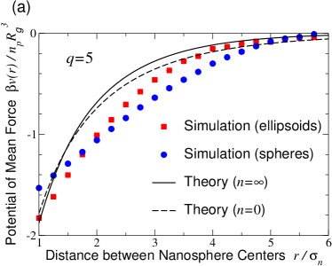
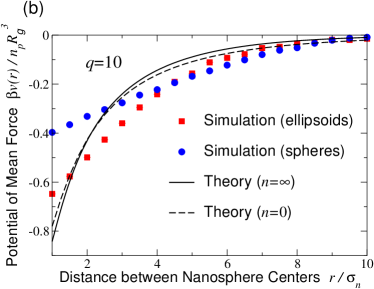
Figure 2 presents direct comparisons of our simulation data with predictions of two polymer field theories Eisenriegler et al. (2003); Wang et al. (2014) for size ratios $q=5$ and $q=10$. The two theories make slightly different predictions, since one Eisenriegler et al. (2003) describes monodisperse coils [$n=\infty$ in Eq. (33)] and the other Wang et al. (2014) polydisperse coils ($n=0$). (When replotted in Fig. 2, the pair potentials from ref. Wang et al. (2014) have been corrected for a missing scale factor Forsman (2015).) With no fitting parameters, the ellipsoidal polymer model yields a PMF in good agreement with field theories, although with somewhat less curvature. In contrast, the penetrable spherical polymer model, with penetration free energy given by Eq. (12), produces a PMF with a shallower attractive well and a qualitatively different shape. For reference, the AOV model of impenetrable spherical polymer greatly overestimates the depth of the attraction, yielding contact values of $\beta v_{\rm mf}(\sigma_{n})/(n_{p}R_{g}^{3})=5.4$ for $q=5$ and 4.8 for $q=10$ – hardly surprising in the protein limit, where polymers are far from impenetrable. Quantitative discrepancies between simulation and theory, especially at intermediate distances, may originate from the step-function approximation for the polymer-nanoparticle penetration energy profile.

Evidently, polymer shape fluctuations and penetrability both play vital roles in depletion-induced interactions. In passing, we note that using $\beta\varepsilon=3/q$ as the penetration energy for the ellipsoidal polymer model leads to a much weaker pair attraction. Close agreement between polymer field theory predictions and the potentials output by our simulations, which use as input the penetration free energy predicted by the same theory, not only validates the ellipsoidal polymer model, but also confirms the self-consistency of the field theories. We emphasize, however, that our approach, unlike the field theories, can be applied also in the colloid limit Lim and Denton (2015).

Figure 3: Snapshot from simulation of polymer-nanoparticle mixture for computing shape distribution of ellipsoidal polymer immersed in a concentrated dispersion of nanospheres.

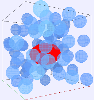
In the second series of simulations, using the eigenvalue distributions of an uncrowded polymer [Eqs. (5) and (6)], we computed the shape distributions of polymers immersed in bulk dispersions of nanospheres of various concentrations (Fig. 3). For both polymers and nanospheres, the tolerance for trial displacements was fixed at 0.1 $\sigma_{n}$. Extending our preliminary study of crowding Lim and Denton (2014), we implemented an exact polymer-nanosphere overlap algorithm Hart (1994) and used a more realistic penetration free energy $\varepsilon$ [Eqs. (11) and (15)]. Since $\varepsilon$ depends, at each nanosphere volume fraction $\phi_{n}$, on the average volume of the crowded polymer $v_{p}(\phi_{n})$, which itself depends on $\varepsilon$, we input the $v_{p}(\phi_{n})$ predicted by free-volume theory and subsequently checked for self-consistency.

In each of the five independent runs, we accumulated configurational data over $10^{7}$ steps, following an equilibration stage of $5\times 10^{4}$ MC steps, and calculated the polymer gyration tensor eigenvalue distributions, asphericity, and rms radius of gyration by averaging over $10^{4}$ independent configurations, spaced by intervals of $10^{3}$ steps to minimize correlations. We typically chose $N_{n}=216$, but performed runs with up to 1728 nanospheres to ensure statistical independence of system size. In the process, we confirmed that our previous approximation Lim and Denton (2014) for the shape of the intersection region as a “stretched” ellipsoid – an ellipsoid whose principal radii are lengthened by $R_{n}$ – is quite reasonable in the protein limit and gives qualitatively consistent results. Results reported below are compared with predictions of free-volume theory. To our knowledge, no corresponding data from simulations of explicit polymer models are yet available for direct comparison.

Figure 4: Probability distributions for the eigenvalues of the gyration tensor of a crowded polymer, modeled as an ideal, freely-jointed chain: (a) $\lambda_{1}$, (b) $\lambda_{2}$, (c) $\lambda_{3}$. Our simulation data (symbols) are compared with predictions of free-volume theory (solid curves) for a single ellipsoidal polymer, with uncrowded rms radius of gyration equal to five times the nanoparticle radius ($q=5$), amidst $N_{n}=216$ hard nanospheres with volume fraction $\phi_{n}=0.1$ (triangles), 0.2 (squares), and 0.3 (circles). Dashed curves show uncrowded distributions ($\phi_{n}=0$) from Eqs. (5) and (6).

Figure 5: Same as Fig. 4, but for larger polymer-to-nanosphere size ratio ($q=10$). Notice the changes in scale.

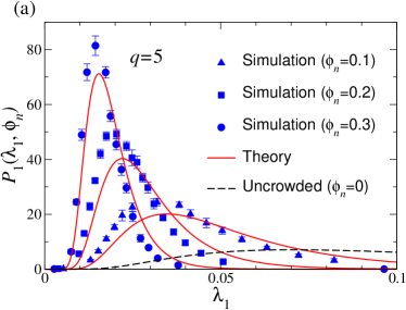
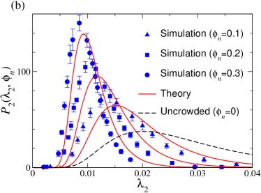
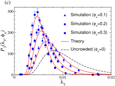
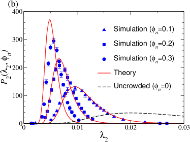
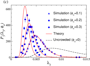
For a polymer immersed in a nanosphere dispersion, with uncrowded rms radius of gyration equal to five times the nanosphere radius ($q=5$), Fig. 4 presents the probability distributions for the eigenvalues of the gyration tensor, representing the distribution of shapes of the ellipsoid that best fits the polymer coil. A comparison of the scales of the distributions for the three eigenvalues reveals that the typical shape of the polymer is that of an elongated, flattened ellipsoid. With increasing crowding, i.e., nanosphere concentration, all three eigenvalue distributions steadily shift toward smaller ranges, reflecting contraction of the polymer along all three principle axes. Also shown in Fig. 4 are predictions of free-volume theory (Sec. III.3). At lower nanosphere concentrations, simulation and theory agree closely. With increasing crowding, however, small deviations emerge, especially notable for the largest eigenvalue $\lambda_{1}$.

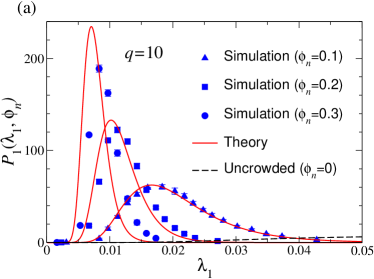
Figure 5 shows the probability distributions for a polymer doubled in size ($q=10$). Compared with the smaller polymer, for the same nanosphere concentration, the shifts in the eigenvalue distributions are significantly larger relative to the uncrowded distributions. As discussed in ref. Lim and Denton (2014), this trend can be understood by noting that the average overlap free energy increases roughly with the square of the size ratio. Also apparent is that the free-volume theory is less accurate for this larger size ratio, somewhat overpredicting the polymer compression, especially at the highest volume fraction.

Figure 6: (a) Asphericity [Eq. (7)], (b) rms radius of gyration [Eq. (8)], and (c) average volume [Eq. (15)] of a fluctuating ellipsoidal polymer vs. nanosphere volume fraction $\phi_{n}$. Our simulation data are shown for uncrowded polymer-to-nanosphere size ratio $q=5$ (circles) and $q=10$ (squares) and compared with predictions of free-volume theory (curves). Error bars are smaller than symbols. As crowding increases, the polymer becomes more compact (smaller and less aspherical). Inset to panel (b): Comparison with scaling prediction Odijk (2000), $R_{g}\sim\phi_{n}^{-1/4}$, on a log-log scale.

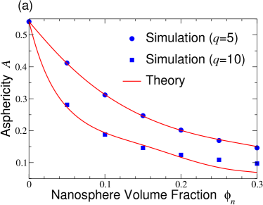
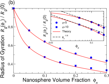
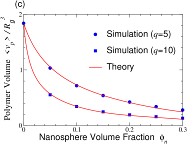
From the eigenvalue distributions, we computed the asphericity [Eq. (7)], rms radius of gyration [Eq. (8)], and average volume [Eq. (15)] of a crowded polymer over a range of nanosphere concentrations. As Fig. 6 demonstrates, a polymer responds to progressive crowding not only by contracting, but also by becoming more spherical, as reflected by the decrease in $A$, $R_{g}$, and $v_{p}$ with increasing $\phi_{n}$. These trends are amplified upon increasing the size ratio from $q=5$ to $q=10$, the larger polymer being relatively more compactified. Moreover, the crowding effect is much stronger here, where we computed $\varepsilon$ from Eqs. (11) and (15), than in our previous study Lim and Denton (2014), where we used lower penetration free energies. Nevertheless, a model of spherical, compressible polymers gives yet greater contraction Lu and Denton (2011); Lim and Denton (2014), which is attributable to the lack of freedom of a spherical polymer to distort its shape.

Figure 6 also shows a comparison of our simulation data with predictions of free-volume theory. As with the eigenvalue distributions, the theory faithfully captures the trends in shape, size, and volume. The inset to panel (b) shows a further comparison with the scaling prediction of Odijk Odijk (2000) for the radius of gyration, $R_{g}\sim\phi_{n}^{-1/4}$, which is seen to be fairly consistent with our data over a significant range of nanosphere concentrations. Here the close agreement between the input (theory) and output (simulation) values of $v_{p}$ serves as a consistency check on our approximation for the penetration free energy. In the coarse-grained polymer model, for the size ratios studied here, neither simulation nor theory indicates a sudden collapse of an ideal coil up to volume fractions $\phi_{n}\simeq 0.4$.

V Conclusions

In summary, to investigate influences of polymer shape and penetrability on mixtures of hard nanospheres and nonadsorbing homopolymers, modeled as penetrable ellipsoids with fluctuating shapes, we developed a Monte Carlo simulation method based on polymer insertion and geometric overlap algorithms. We applied our method to compute depletion-induced potentials of mean force between nanospheres and crowding-induced shape deformations of ideal polymers in the protein limit. Our simulation data for pair interactions are in good agreement with predictions of polymer field theories, further validating the ellipsoidal polymer model and demonstrating the importance of polymer shape fluctuations and penetrability for depletion interactions. Our results for shape distributions of crowded polymers, including asphericity and rms radius of gyration, agree closely with predictions of free-volume theory, differing quantitatively only in highly concentrated nanosphere dispersions. Extending our previous study Lim and Denton (2014), we consistently incorporated the dependence of the penetration free energy on the polymer shape and nanoparticle concentration. Furthermore, our predictions for polymer shape deformations can be tested against molecular simulations or density-functional theory calculations for explicit segmented-chain polymers, which may guide refinement of the step-function approximation assumed for the penetration energy profile.

The methods and results presented here lay a foundation for simulating more realistic models of polymer-nanoparticle mixtures, as well as models of polymers in quenched disordered media  Edwards and Muthukumar (1988); Cates and Ball (1988); Goldschmidt (2000). Future work will focus on generalizing the model from ideal polymers to nonideal polymers in good solvents with excluded-volume interactions Bolhuis et al. (2003); Doxastakis et al. (2004, 2005) characterized by shape distributions of self-avoiding random walks Sciutto (1996); Schäfer (1999), analyzing crowding of real biopolymers Goldenberg (2003); Dima and Thirumalai (2004); Cheung et al. (2005); Denesyuk and Thirumalai (2011, 2013a) (e.g., specific proteins and RNA), and exploring influences of polymer shape fluctuations on thermodynamic stability and phase behavior (e.g., demixing) of bulk polymer-nanoparticle mixtures.

References

- Lekkerkerker and Tuinier (2011) H. N. W. Lekkerkerker and R. Tuinier, Colloids and the Depletion Interaction (Springer, Heidelberg, 2011).
- Balazs et al. (2006) A. C. Balazs, T. Emrick, and T. P. Russell, Science 314, 1107 (2006).
- Mackay et al. (2006) M. E. Mackay, A. Tuteja, P. M. Duxbury, C. J. Hawker, B. Van Horn, Z. Guan, G. Chen, and R. S. Krishnan, Science 311, 1740 (2006).
- Asakura and Oosawa (1954) S. Asakura and F. Oosawa, J. Chem. Phys. 22, 1255 (1954).
- de Gennes (1979) P. G. de Gennes, Scaling Concepts in Polymer Physics (Cornell, Ithaca, 1979).
- Israelachvili (1992) J. Israelachvili, Intermolecular and Surface Forces (Academic, London, 1992).
- Vrij (1976) A. Vrij, Pure & Appl. Chem. 48, 471 (1976).
- Pusey (1991) P. N. Pusey, “Colloidal Suspensions,” in Liquids, Freezing and Glass Transition, Les Houches session 51, Vol. 2, edited by J.-P. Hansen, D. Levesque, and J. Zinn-Justin (North-Holland, Amsterdam, 1991) pp. 763–931.
- Jones (2002) R. A. L. Jones, Soft Condensed Matter (Oxford, Oxford, 2002).
- Fuchs and Schweizer (2002) M. Fuchs and K. S. Schweizer, J. Phys.: Condens. Matter 14, R239 (2002).
- Fleer and Tuinier (2008) G. J. Fleer and R. Tuinier, Adv. Coll. Interface Sci. 143, 1 (2008).
- Denton (2007) A. R. Denton, “Effective Interactions in Soft Materials,” in Nanostructured Soft Matter: Experiment, Theory, Simulation and Perspectives, edited by A. V. Zvelindovsky (Springer, Dordrecht, 2007) pp. 395–433.
- Tolstoguzov (1991) V. B. Tolstoguzov, Food Hydrocolloids 4, 429 (1991).
- de Kruif and Tuinier (2001) C. de Kruif and R. Tuinier, Food Hydrocolloids 15, 555 (2001).
- Norde (2011) W. Norde, Colloids and Interfaces in Life Sciences and Bionanotechnology, 2nd ed. (CRC, Boca Raton, 2011).
- Dogic et al. (2004) Z. Dogic, K. R. Purdy, E. Grelet, M. Adams, and S. Fraden, Phys. Rev. E 69, 051702 (2004).
- Li et al. (2013) T. Li, X. Zan, Y. Sun, X. Zuo, X. Li, A. Senesi, R. E. Winans, Q. Wang, and B. Lee, Langmuir 29, 12777 (2013).
- Kulkarni and Zukoski (2001) A. Kulkarni and C. Zukoski, J. Crystal Growth 232, 156 (2001).
- Stradner et al. (2007) A. Stradner, G. Foffi, N. Dorsaz, G. Thurston, and P. Schurtenberger, Phys. Rev. Lett. 99, 198103 (2007).
- Minton (1981) A. P. Minton, Biopolymers 20, 2093 (1981).
- Minton (2000) A. P. Minton, Biophys. J. 78, 101 (2000).
- Minton (2001) A. P. Minton, J. Biol. Chem. 276, 10577 (2001).
- Richter et al. (2007) K. Richter, M. Nessling, and P. Lichter, J. Cell Sci. 120, 1673 (2007).
- Richter et al. (2008) K. Richter, M. Nessling, and P. Lichter, Biochim. Biophys. Acta 1783, 2100 (2008).
- Elcock (2010) A. H. Elcock, Current Opin. Struct. Biol. 20, 1 (2010).
- Hancock (2012) R. Hancock, in Genome Organization and Function in the Cell Nucleus, edited by K. Rippe (Wiley-VCH, Weinheim, 2012) pp. 169–184.
- Kuhn (1934) W. Kuhn, Kolloid-Zeitschrift 68, 2 (1934).
- Fixman (1962) M. Fixman, J. Chem. Phys. 36, 306 (1962).
- Flory and Fisk (1966) P. J. Flory and S. Fisk, J. Chem. Phys. 44, 2243 (1966).
- Flory (1969) P. J. Flory, Statistical Mechanics of Chain Molecules (Wiley, New York, 1969).
- Yamakawa (1970) H. Yamakawa, Modern Theory of Polymer Solutions (Harper & Row, New York, 1970).
- Fujita and Norisuye (1970) H. Fujita and T. Norisuye, J. Chem. Phys. 52, 1115 (1970).
- Šolc (1971) K. Šolc, J. Chem. Phys. 55, 335 (1971).
- Šolc (1973) K. Šolc, Macromol. 6, 378 (1973).
- Theodorou and Suter (1985) D. N. Theodorou and U. W. Suter, Macromol. 18, 1206 (1985).
- Rudnick and Gaspari (1986) J. Rudnick and G. Gaspari, J. Phys. A: Math. Gen. 19, L191 (1986).
- Rudnick and Gaspari (1987) J. Rudnick and G. Gaspari, Science 237, 384 (1987).
- Bishop and Saltiel (1988) M. Bishop and C. J. Saltiel, J. Chem. Phys. 88, 6594 (1988).
- Sciutto (1996) S. J. Sciutto, J. Phys. A: Math. Gen. 29, 5455 (1996).
- Schäfer (1999) L. Schäfer, Excluded Volume Effects in Polymer Solutions as Explained by the Renormalization Group (Springer, Berlin, 1999).
- Murat and Kremer (1998) M. Murat and K. Kremer, J. Chem. Phys. 108, 4340 (1998).
- Eurich and Maass (2001) F. Eurich and P. Maass, J. Chem. Phys. 114, 7655 (2001).
- Ellis (2001a) R. J. Ellis, Current Opin. Struct. Biol. 11, 114 (2001a).
- Ellis (2001b) R. J. Ellis, Trends in Biochem. Sci. 261, 597 (2001b).
- van der Maarel (2008) J. R. C. van der Maarel, Introduction to Biopolymer Physics (World Scientific, Singapore, 2008).
- Phillips et al. (2009) R. Phillips, J. Kondev, and J. Theriot, Physical Biology of the Cell (Garland Science, New York, 2009).
- Cheung (2013) M. S. Cheung, Current Opin. Struct. Biol 23, 1 (2013).
- Denton (2013) A. R. Denton, in New Models of the Cell Nucleus: Crowding and Entropic Forces and Phase Separation and Fractals, edited by R. Hancock and K. W. Jeon (Academic Press, UK, 2013) pp. 27–72.
- Ali et al. (2006) I. Ali, D. Marenduzzo, and J. M. Yeomans, Phys. Rev. Lett. 96, 208102 (2006).
- Polson et al. (2013) J. M. Polson, M. F. Hassanabad, and A. McCaffrey, J. Chem. Phys. 138, 024906 (2013).
- Ye et al. (1996) X. Ye, T. Narayanan, P. Tong, and J. S. Huang, Phys. Rev. Lett. 76, 4640 (1996).
- Nakatani et al. (2001) A. I. Nakatani, W. Chen, R. G. Schmidt, G. V. Gordon, and C. C. Han, Polymer 42, 3713 (2001).
- Kramer et al. (2005a) T. Kramer, R. Schweins, and K. Huber, J. Chem. Phys. 123, 014903 (2005a).
- Kramer et al. (2005b) T. Kramer, R. Schweins, and K. Huber, Macromol. 38, 151 (2005b).
- Kramer et al. (2005c) T. Kramer, R. Schweins, and K. Huber, Macromol. 38, 9783 (2005c).
- Le Coeur et al. (2009) C. Le Coeur, B. Demé, and S. Longeville, Phys. Rev. E 79, 031910 (2009).
- Le Coeur et al. (2010) C. Le Coeur, J. Teixeira, P. Busch, and S. Longeville, Phys. Rev. E 81, 061914 (2010).
- Nusser et al. (2010) K. Nusser, S. Neueder, G. J. Schneider, M. Meyer, W. Pyckhout-Hintzen, L. Willner, A. Radulescu, and D. Richter, Macromol. 43, 9837 (2010).
- Milling and Biggs (1995) A. Milling and S. Biggs, J. Colloid Interface Sci. 170, 604 (1995).
- Rudhardt et al. (1998) D. Rudhardt, C. Bechinger, and P. Leiderer, Phys. Rev. Lett. 81, 1330 (1998).
- Verma et al. (1998) R. Verma, J. C. Crocker, T. C. Lubensky, and A. G. Yodh, Phys. Rev. Lett. 81, 4004 (1998).
- Lin et al. (2001) K. H. Lin, J. C. Crocker, A. C. Zeri, and A. G. Yodh, Phys. Rev. Lett. 87, 088301 (2001).
- Hilitski et al. (2015) F. Hilitski, A. R. Ward, L. Cajamarca, M. F. Hagan, G. M. Grason, and Z. Dogic, Phys. Rev. Lett. 114, 138102 (2015).
- Hennequin et al. (2005) Y. Hennequin, M. Evens, C. M. Q. Angulo, and J. S. van Duijneveldt, J. Chem. Phys. 123, 054906 (2005).
- Zhang and van Duijneveldt (2006) Z. Zhang and J. S. van Duijneveldt, Langmuir 22, 63 (2006).
- Mutch et al. (2007) K. J. Mutch, J. S. van Duijneveldt, and J. Eastoe, Soft Matter 3, 155 (2007).
- Joanny et al. (1979) J. F. Joanny, L. Leibler, and P. G. de Gennes, J. Polymer Sci.: Polymer Phys. Ed. 17, 1073 (1979).
- Sear (1997) R. P. Sear, Phys. Rev. E 56, 4463 (1997).
- Sear (2001) R. P. Sear, Phys. Rev. Lett. 86, 4696 (2001).
- Sear (2002) R. P. Sear, Phys. Rev. E 66, 51401 (2002).
- Minton (2005) A. P. Minton, Biophys. J. 88, 971 (2005).
- Denton and Schmidt (2002) A. R. Denton and M. Schmidt, J. Phys.: Condens. Matter 14, 12051 (2002).
- Lu and Denton (2011) B. Lu and A. R. Denton, J. Phys.: Condens. Matter 23, 285102 (2011).
- Lim and Denton (2014) W. K. Lim and A. R. Denton, J. Chem. Phys. 141, 114909 (2014).
- Walz and Sharma (1994) J. Y. Walz and A. Sharma, J. Colloid Interface Sci. 168, 485 (1994).
- Mao et al. (1995) Y. Mao, M. E. Cates, and H. N. W. Lekkerkerker, Physica A 222, 10 (1995).
- Mao et al. (1997) Y. Mao, M. E. Cates, and H. N. W. Lekkerkerker, J. Chem. Phys. 106, 3721 (1997).
- Eisenriegler et al. (1996) E. Eisenriegler, A. Hanke, and S. Dietrich, Phys. Rev. E 54, 1134 (1996).
- Hanke et al. (1999) A. Hanke, E. Eisenriegler, and S. Dietrich, Phys. Rev. E 59, 6853 (1999).
- Eisenriegler et al. (2003) E. Eisenriegler, A. Bringer, and R. Maassen, J. Chem. Phys. 118, 8093 (2003).
- Odijk (2000) T. Odijk, Physica A 278, 347 (2000).
- Woodward and Forsman (2010) C. E. Woodward and J. Forsman, J. Chem. Phys. 133, 154902 (2010).
- Woodward and Forsman (2012) C. E. Woodward and J. Forsman, J. Chem. Phys. 136, 084903 (2012).
- Wang et al. (2014) H. Wang, C. E. Woodward, and J. Forsman, J. Chem. Phys. 140, 194903 (2014).
- Chatterjee and Schweizer (1998) A. P. Chatterjee and K. S. Schweizer, J. Chem. Phys. 109, 10464 (1998).
- Ramakrishnan et al. (2002) S. Ramakrishnan, M. Fuchs, K. S. Schweizer, and C. F. Zukoski, J. Chem. Phys. 116, 2201 (2002).
- Moncho-Jordá et al. (2003) A. Moncho-Jordá, A. A. Louis, P. G. Bolhuis, and R. Roth, J. Phys.: Condens. Matter 15, S3429 (2003).
- Bechinger et al. (1999) C. Bechinger, D. Rudhardt, P. Leiderer, R. Roth, and S. Dietrich, Phys. Rev. Lett. 83, 3960 (1999).
- Schmidt and Fuchs (2002) M. Schmidt and M. Fuchs, J. Chem. Phys. 117, 6308 (2002).
- Goel et al. (2004) T. Goel, C. N. Patra, S. K. Ghosh, and T. Mukherjee, J. Chem. Phys. 121, 4865 (2004).
- Woodward and Forsman (2008) C. E. Woodward and J. Forsman, Phys. Rev. Lett. 100, 098301 (2008).
- Forsman and Woodward (2009) J. Forsman and C. E. Woodward, J. Chem. Phys. 131, 044903 (2009).
- Tuinier et al. (2000) R. Tuinier, G. A. Vliegenthart, and H. N. W. Lekkerkerker, J. Chem. Phys. 113, 10768 (2000).
- Tuinier and Lekkerkerker (2001) R. Tuinier and H. N. W. Lekkerkerker, Eur. Phys. J. E 6, 129 (2001).
- Tuinier and Petukhov (2002) R. Tuinier and A. V. Petukhov, Macromol. Theory Simul. 11, 975 (2002).
- Meijer and Frenkel (1991) E. J. Meijer and D. Frenkel, Phys. Rev. Lett. 67, 1110 (1991).
- Meijer and Frenkel (1994) E. J. Meijer and D. Frenkel, J. Chem. Phys. 100, 6873 (1994).
- Dickman and Yethiraj (1994) R. Dickman and A. Yethiraj, J. Chem. Phys. 100, 4683 (1994).
- Bolhuis et al. (2002) P. G. Bolhuis, A. A. Louis, and J.-P. Hansen, Phys. Rev. Lett. 89, 128302 (2002).
- Louis et al. (2002) A. A. Louis, P. G. Bolhuis, E. J. Meijer, and J.-P. Hansen, J. Chem. Phys. 117, 1893 (2002).
- Bolhuis et al. (2003) P. G. Bolhuis, E. J. Meijer, and A. A. Louis, Phys. Rev. Lett. 90, 068304 (2003).
- Doxastakis et al. (2004) M. Doxastakis, Y. L. Chen, O. Guzmán, and J. J. de Pablo, J. Chem. Phys. 120, 9335 (2004).
- Doxastakis et al. (2005) M. Doxastakis, Y. L. Chen, and J. J. de Pablo, J. Chem. Phys. 123, 34901 (2005).
- Goldenberg (2003) D. P. Goldenberg, J. Mol. Biol. 326, 1615 (2003).
- Dima and Thirumalai (2004) R. I. Dima and D. Thirumalai, J. Phys. Chem. B 108, 6564 (2004).
- Cheung et al. (2005) M. Cheung, D. Klimov, and D. Thirumalai, Proc. Natl. Acad. Sci 102, 4753 (2005).
- Denesyuk and Thirumalai (2011) N. A. Denesyuk and D. Thirumalai, J. Am. Chem. Soc. 133, 11858 (2011).
- Denesyuk and Thirumalai (2013a) N. A. Denesyuk and D. Thirumalai, Biophys. Rev. 5, 225 (2013a).
- Camargo and Likos (2010) M. Camargo and C. N. Likos, Phys. Rev. Lett. 104, 078301 (2010).
- Linhananta et al. (2012) A. Linhananta, G. Amadei, and T. Miao, J. Phys.: Conf. Ser. 341, 012009 (2012).
- Chen et al. (2012) E. Chen, A. Christiansen, Q. Wang, M. S. Cheung, D. S. Kliger, and P. Wittung-Stafshede, Biochem. 51, 9836 (2012).
- Hoppe and Yuan (2011) T. Hoppe and J.-M. Yuan, J. Phys. Chem. B 115, 2006 (2011).
- Denesyuk and Thirumalai (2013b) N. A. Denesyuk and D. Thirumalai, J. Phys. Chem. B 117, 4901 (2013b).
- Triantafillou and Kamien (1999) M. Triantafillou and R. D. Kamien, Phys. Rev. E 59, 5621 (1999).
- Piech and Walz (2000) M. Piech and J. Y. Walz, J. Colloid Interface Sci. 232, 86 (2000).
- Lim and Denton (2015) W. K. Lim and A. R. Denton, Soft Matter (2015), 10.1039/C5SM02863A.
- Eurich et al. (2007) F. Eurich, A. Karatchentsev, J. Baschnagel, W. Dieterich, and P. Maass, J. Chem. Phys. 127, 134905 (2007).
- Frenkel and Smit (2001) D. Frenkel and B. Smit, Understanding Molecular Simulation, 2nd ed. (Academic, London, 2001).
- Binder and Heermann (2010) K. Binder and D. W. Heermann, Monte Carlo Simulation in Statistical Physics: An Introduction, 5th ed. (Springer, Berlin, 2010).
- Hart (1994) J. C. Hart, in Graphics Gems IV, edited by P. S. Heckbert (Academic, San Diego, 1994) pp. 113–119.
- Widom (1963) B. Widom, J. Chem. Phys. 39, 2808 (1963).
- Oversteegen and Roth (2005) S. M. Oversteegen and R. Roth, J. Chem. Phys. 122, 214502 (2005).
- Rosenfeld (1989) Y. Rosenfeld, Phys. Rev. Lett. 63, 980 (1989).
- Rosenfeld et al. (1997) Y. Rosenfeld, M. Schmidt, H. Löwen, and P. Tarazona, Phys. Rev. E 55, 4245 (1997).
- Schmidt et al. (2000) M. Schmidt, H. Löwen, J. M. Brader, and R. Evans, Phys. Rev. Lett 85, 1934 (2000).
- Lebowitz et al. (1964) J. L. Lebowitz, E. Helfand, and E. Praestgaard, J. Chem. Phys. 43, 774 (1964).
- Hansen and McDonald (2006) J.-P. Hansen and I. R. McDonald, Theory of Simple Liquids, 3rd ed. (Elsevier, London, 2006).
- Forsman (2015) J. Forsman, private communication (2015).
- Edwards and Muthukumar (1988) S. F. Edwards and M. Muthukumar, J. Chem. Phys. 89, 2435 (1988).
- Cates and Ball (1988) M. E. Cates and C. Ball, J. Phys. France 49, 2009 (1988).
- Goldschmidt (2000) Y. Y. Goldschmidt, Phys. Rev. E 61, 1729 (2000).