Computational Pathology: Challenges and Promises for Tissue Analysis
Abstract
The histological assessment of human tissue has emerged as the key challenge for detection and treatment of cancer. A plethora of different data sources ranging from tissue microarray data to gene expression, proteomics or metabolomics data provide a detailed overview of the health status of a patient. Medical doctors need to assess these information sources and they rely on data driven automatic analysis tools. Methods for classification, grouping and segmentation of heterogeneous data sources as well as regression of noisy dependencies and estimation of survival probabilities enter the processing workflow of a pathology diagnosis system at various stages. This paper reports on state-of-the-art of the design and effectiveness of computational pathology workflows and it discusses future research directions in this emergent field of medical informatics and diagnostic machine learning.
keywords:
Computational Pathology , Machine Learning , Medical Imaging , Survival Statistics , Cancer Research1 Computational Pathology: The systems view
Modern pathology studies of biopsy tissue encompass multiple stainings of histological material, genomics and proteomics analyses as well as comparative statistical analyses of patient data. Pathology lays not only a scientific foundation for clinical medicine but also serves as a bridge between the fundamental sciences in natural science, medicine and patient care. Therefore, it can be viewed as one of the key hubs for translational research in the health and life sciences, subsequently facilitating translational medicine. In particular, the abundance of heterogeneous data sources with a substantial amount of randomness and noise poses challenging problems for statistics and machine learning. Automatic processing of this wealth of data promises a standardized and hopefully more objective diagnosis of the disease state of a patient than manual inspection can provide today. An automatic computational pathology pipeline also enables the medical user to quantitatively benchmark the processing pipeline and to identify error sensitive processing steps which can substantially degrade the final prediction of survival times.
1.1 Definition
Computational Pathology as well as the medical discipline Pathology is a wide and diverse field which encompass scientific research as well as day-to-day work in medical clinics. The following definition is an attempt for a concise and practical description of this novel field:
Computational Pathology investigates a complete probabilistic treatment of scientific and clinical workflows in general pathology, i.e. it combines experimental design, statistical pattern recognition and survival analysis to an unified framework for answering scientific and clinical questions in pathology.
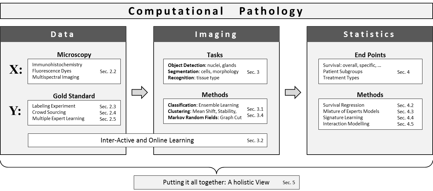
Figure 1 depicts a schematic overview of the field and the three major parts it consists of: data generation, image analysis and medical statistics.
2 Data: Tissue and Ground Truth
2.1 Clear Cell Renal Cell Carcinoma
Throughout this review we use Renal cell carcinoma (RCC) as a disease case to design and optimize a computational pathology framework because it exhibits a number of properties which are highly relevant for computational pathology.
Renal cell carcinoma figures as one of the ten most frequent malignancies in the statistics of Western societies [1]. The prognosis of renal cancer is poor since many patients suffer already from metastases at the time of first diagnosis. The identification of biomarkers for prediction of prognosis (prognostic marker) or response to therapy (predictive marker) is therefore of utmost importance to improve patient prognosis [2]. Various prognostic markers have been suggested in the past [3, 4], but estimates of conventional morphological parameters still provide most valuable information for therapeutical decisions.
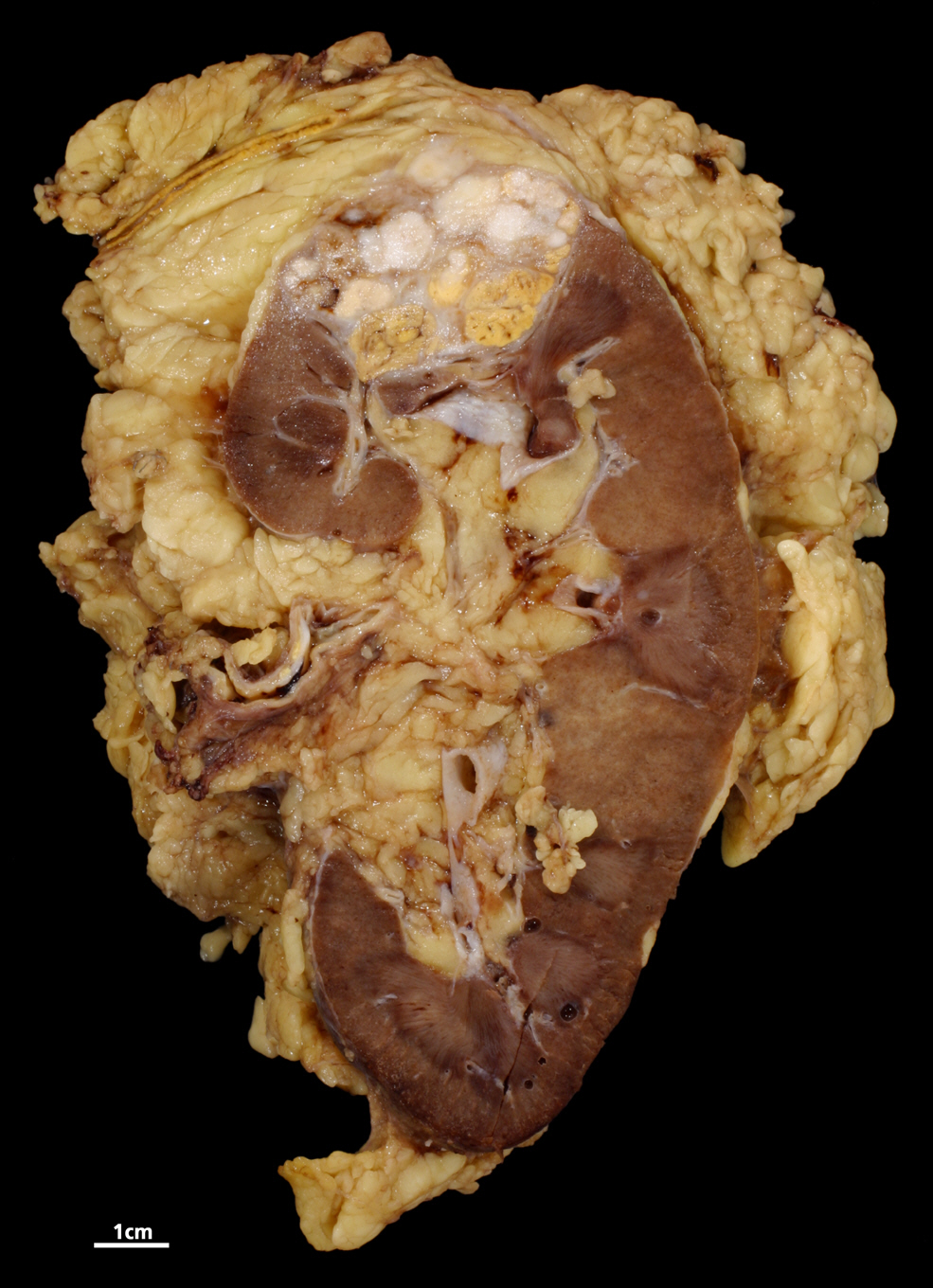
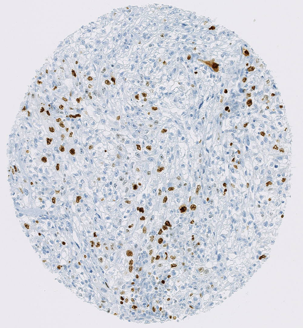
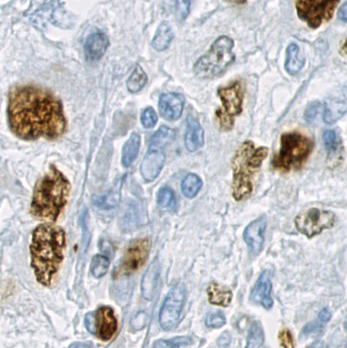
Clear cell RCC (ccRCC) emerged as the most common subtype of renal cancer and it is composed of cells with clear cytoplasm and typical vessel architecture. ccRCC exhibits an architecturally diverse histological structure, with solid, alveolar and acinar patterns. The carcinomas typically contain a regular network of small thin-walled blood vessels, a diagnostically helpful characteristic of this tumor. Most ccRCC show areas with hemorrhage or necrosis (Fig. 2d), whereas an inflammatory response is infrequently observed. Nuclei tend to be round and uniform with finely granular and evenly distributed chromatin. Depending upon the grade of malignancy, nucleoli may be inconspicuous and small, or large and prominent, with possibly very large nuclei or bizarre nuclei occurring [1].
The prognosis for patients with RCC depends mainly on the pathological stage and the grade of the tumor at the time of surgery. Other prognostic parameters include proliferation rate of tumor cells and different gene expression patterns. Tannapfel et al. [2] have shown that cellular proliferation potentially serves as another measure for predicting biological aggressiveness and, therefore, for estimating the prognosis. Immunohistochemical assessment of the MIB-1 (Ki-67) antigen indicates that MIB-1 immunostaining (Fig. 2d) is an additional prognostic parameter for patient outcome. TMAs were highly representative of proliferation index and histological grade using bladder cancer tissue [5].
The TNM staging system specifies the local extension of the primary tumour (T), the involvement of regional lymph nodes (N), and the presence of distant metastases (M) as indicators of the disease state. [6] focuses on reassessing the current TNM staging system for RCC and concludes that outcome prediction for RCC remains controversial. Although many parameters have been tested for prognostic significance, only a few have achieved general acceptance in clinical practice. An especially interesting observation of [6] is that multivariate Cox proportional hazards regression models including multiple clinical and pathologic covariates were more accurate in predicting patient outcome than the TNM staging system. On one hand this finding demonstrates the substantial difficulty of the task and on the other hand it is a motivation for research in computational pathology to develop robust machine learning frameworks for reliable and objective prediction of disease progression.
2.2 Tissue Microarrays
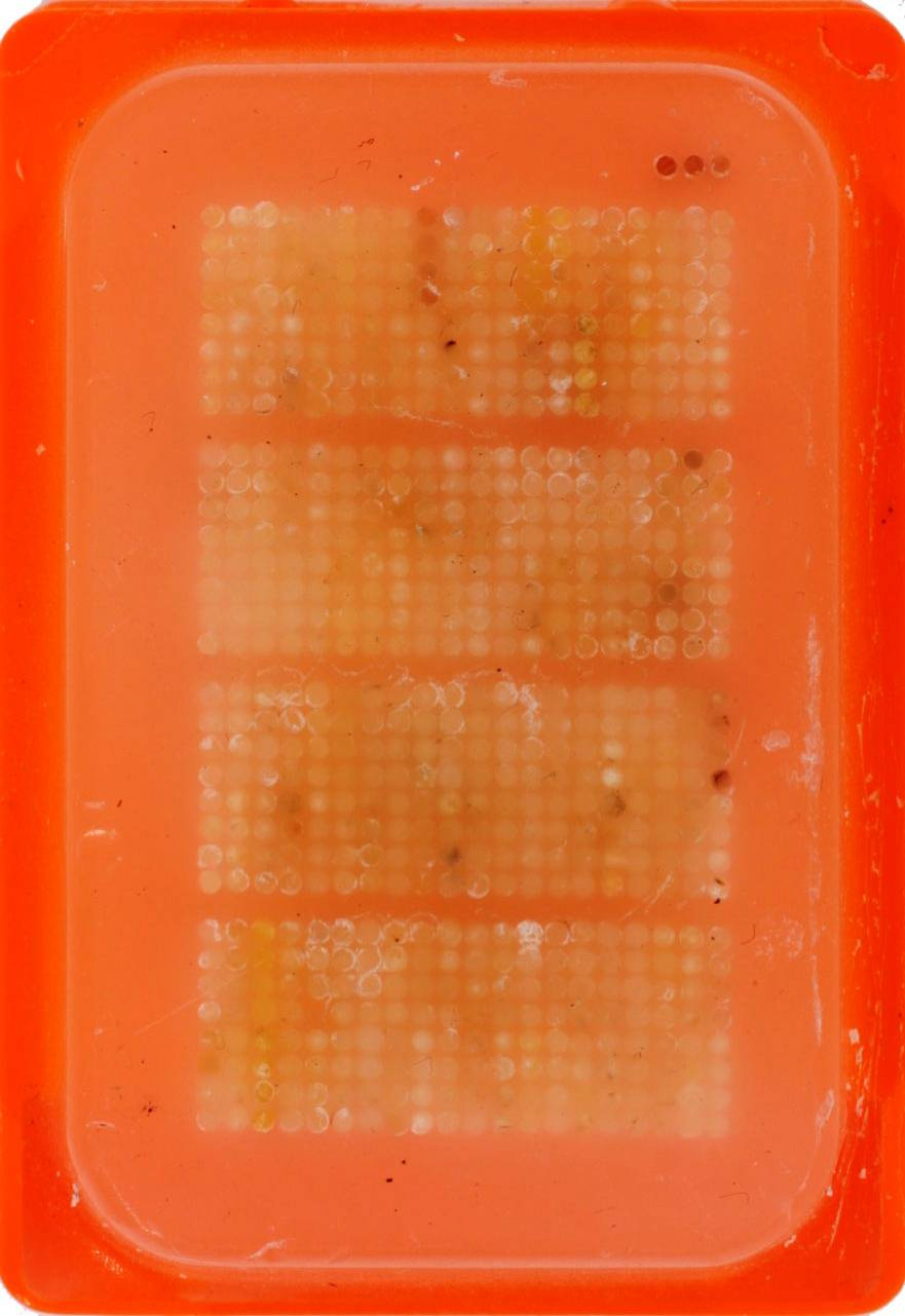
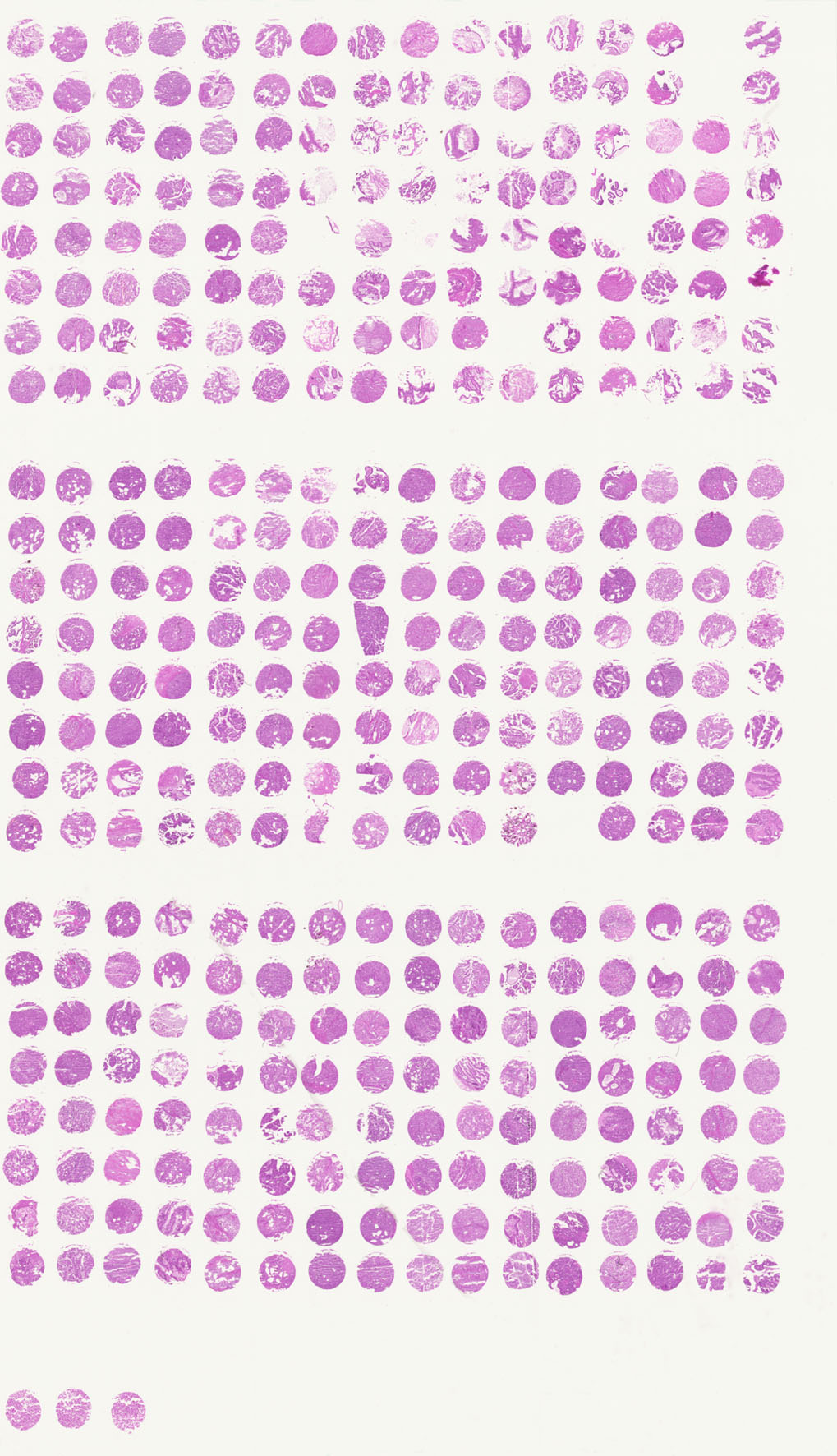
The tissue microarray (TMA) technology significantly accelerated studies seeking for associations between molecular changes and clinical endpoints [7]. In this technology, tissue cylinders are extracted from primary tumor material of hundreds of different patients and these cylinders are subsequently embedded into a recipient tissue block. Sections from such array blocks can then be used for simultaneous in situ analysis of hundreds or thousands of primary tumors on DNA, RNA, and protein level (cf. 2). These results can then be integrated with expression profile data which is expected to enhance the diagnosis and prognosis of ccRCC [8, 3, 9]. The high speed of arraying, the lack of a significant damage to donor blocks, and the regular arrangement of arrayed specimens substantially facilitates automated analysis.
 |
 |
 |
 |
 |
| (a) | (b) | (c) | (d) | (e) |
Although the production of tissue microarrays is an almost routine task for most laboratories, the evaluation of stained tissue microarray slides remains tedious human annotation work, it is time consuming and prone to error. Furthermore, the significant intratumoral heterogeneity of RCC results in high interobserver variability. The variable architecture of RCC also results in a difficult assessment of prognostic parameters. Current image analysis software requires extensive user interaction to properly identify cell populations, to select regions of interest for scoring, to optimize analysis parameters and to organize the resulting raw data. Because of these drawbacks in current software, pathologists typically collect tissue microarray data by manually assigning a composite staining score for each spot - often during multiple microscopy sessions over a period of days. Such manual scoring can result in serious inconsistencies between data collected during different microscopy sessions. Manual scoring also introduces a significant bottleneck that hinders the use of tissue microarrays in high-throughput analysis.
2.3 Analyzing Pathologists
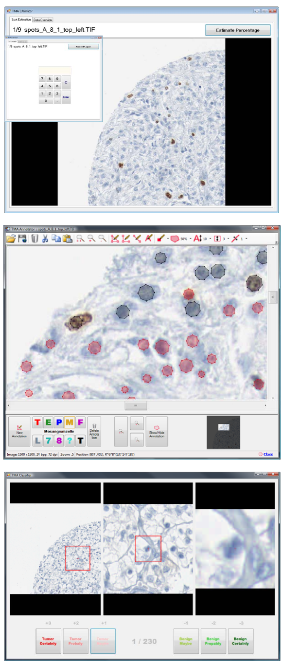
To assess the inter and intra variability of pathologists we designed three different labeling experiments for the major tasks involved in TMA analysis. To facilitate the labeling process for trained pathologists we developed software suite which allows the user to view single TMA spots and which provides zooming and scrolling capabilities. The expert can annotate the image with vectorial data in SVG (support vector graphics) format and he/she can mark cell nuclei, vessels and other biological structures. In addition each structure can be labeled with a class which is encoded by its color. To increase usability and the adoption in hospitals we specifically designed the software for tablet PC so that a pathologist can perform all operations with a pen alone in a simple and efficient manner. Figure 3 depicts the graphical user interfaces of the three applications.
 |
 |
| (a) | (b) |
 |
 |
| (c) | (d) |
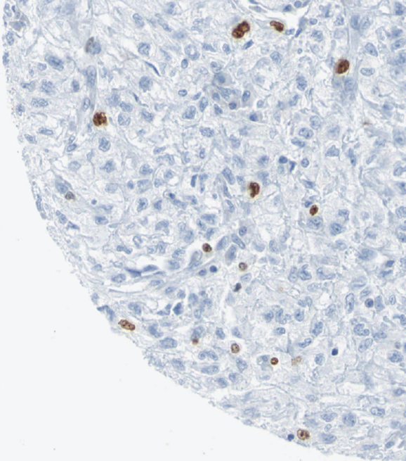
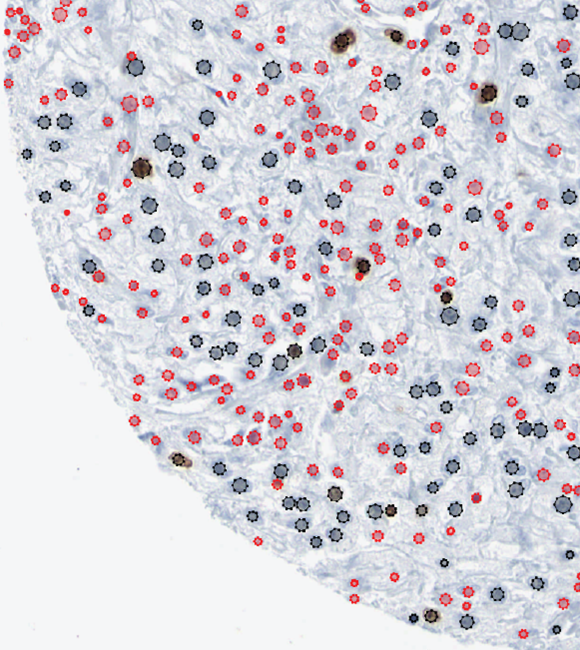
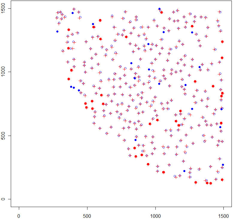
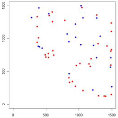
Nuclei Detection: The most tedious labeling task is the detection of cell nuclei. In this experiment two experts on renal cell carcinoma exhaustively labeled a quarter of each of the 9 spots from the previous experiment. Overall each expert independently marked the center, the approximate radius and the class of more than 2000 nuclei. Again a tablet PC was used so it was possible to split up the work into several sessions and the experts could use the machine at their convenience. The user detects nuclei by marking the location with the pen on the tablet and indicates the diameter by moving the pen. A circular semi-transparent polygon is then drawn to mark the nucleus. The final step consists of choosing a class for the nucleus. In this setting it was either black for cancerous nuclei or red for normal ones. This task has to be repeated for each nucleus on each spot. Finally it is possible to show and hide the annotation to gain an overview over the original tissue. Figure 4 depicts a quarter of one of the RCC TMA spots together with the annotation and the inter expert disagreement.
The average precision of one pathologist compared to the other is and the average recall amounts to . These performance numbers show that even detecting nuclei on an histological slide is by far not an easy or undisputed task.
Nuclei Classification: The third experiment was designed to evaluate the inter and intra pathologist variability for nuclei classification, i.e. determining if a nucleus is normal/benign or abnormal/malignant. This step crucially influences the final outcome due to the fact that the percentage of staining is only estimated on the subset of cancerous nuclei. In the experiment, randomly selected nuclei are sequentially presented in three different views of varying zoom stage. The query nucleus is indicated in each view with a red cross and the area which comprises the next zoom view is marked with a red bounding box (cf. Figure 3). During the setup phase the user can adjust these views to simulate his usual workflow as good as possible. During the experiment the expert has to select a class for each nucleus and rate his confidence. Thus, he has the choice between six buttons: tumor certainly, tumor probably, tumor maybe, benign certainly, benign probably and benign maybe. After classifying all nuclei, which have been classified as tumor, are displayed again and the pathologist has to estimate if the nucleus is stained or not. Again he has to rate his confidence in his own decision on a scale of three levels. To test the intra pathologist’s variability a subset of nuclei was queried twice but the images were flipped and rotated by 90 degree at the second display to hamper recognition.
 |
 |
 |
 |
| (a) | (b) | (c) | (d) |
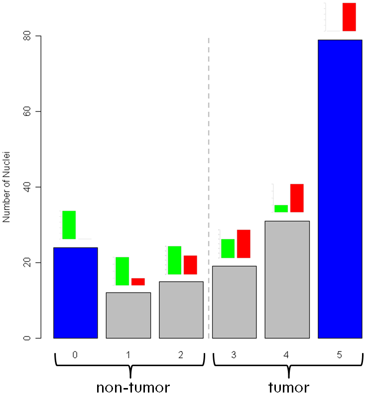
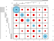
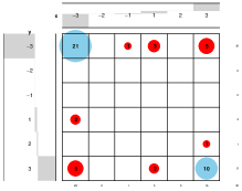
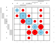
The results for inter-pathologist variability for the binary classification task are plotted in Figure 5a. Out of nuclei all five experts agreed on nuclei to be normal and nuclei to be ab-normal, respectively cancerous. For the other nuclei () the pathologists disagreed.
The analysis of the intra-pathologist error is shown in Figure 5b. The overall intra classification error is This means that every fifth nucleus was classified by an expert first as cancerous and the second time as normal or vice versa. The self-assessment of confidence allows us also to analyze single pathologists. For example Figure 5c shows the results of a very self-confident pathologist who is always very certain of his decisions but ends up with an error of in the replication experiment. Figure 5d on the other hand is the result of a very cautious expert who is rather unsure of his decision, but with a misclassification error of he performs significantly better than the previous one. The important lesson learned is, that self-assessment is not a reliable information to learn from. The intuitive notion, to use only training samples which were classified with high confidence by domain experts is not valid.
In defense of human pathologist it has to be mentioned that these experiments represent the most general way to conduct a TMA analysis and analogous studies in radiology report similar results [10, 11]. In practice, domain experts focus only on regions of TMA spots which are very well processed, which have no staining artifacts or which are not blurred. The nuclei analyzed in this experiment were randomly sampled from the whole set of detected nuclei to mimic the same precondition which an algorithm would encounter in routine work. Reducing the analysis to perfectly processes regions would most probably decrease the intra-pathologist error.
Staining Estimation: The most common task in manual TMA analysis requires to estimate the staining. To this end a domain expert views the spot of a patients for several seconds and estimates the number of stained abnormal cells without resorting to actual nuclei counting. This procedure is iterated for each spot on a TMA-slide to get an estimate for each patient in the study.
It is important to note that, due to the lack of competitive algorithms, the results of nearly all TMA studies are based on this kind of subjective estimations.
 |
 |
| (a) | (b) |
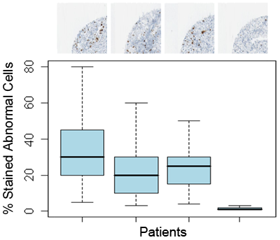
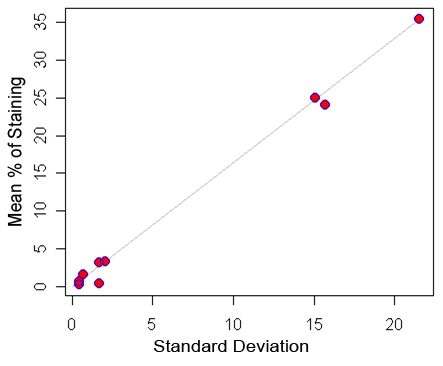
To investigate estimation consistency we presented 9 randomly selected TMA spots to 14 trained pathologists of the University Hospital Zurich.
The estimations of the experts varied by up to as shown in Figure 6b. As depicted in Figure 6b the standard deviation between the experts grows linearly with the average estimated amount of staining. The high variability demonstrates the subjectivity of the estimation process. This uncertainty is especially critical for types of cancer for which the clinician chooses the therapy based on the estimated staining percentage. This result not only motivates but emphasizes the need for more objective estimation procedures than current practice. Our research is stimulated by the hope, that computational pathology approaches do not only automated such estimation processes but also produce better reproduceable and more objective results than human judgment.
2.4 Expert Variability in Fluorescence Microscopy
Complementary to immunohistochemical TMA analysis, fluorescence microscopy is applied often for high-throughput screening of molecular phenotypes. A comprehensive study evaluating the performance of domain experts regarding the detection of lymphocytes is presented by [12]. In a best case, a medium-skilled expert needs on average one hour for analyzing a fluorescence micrograph. Each micrograph contains between 100 and 400 cells and is of size pixel. Four exemplary micrographs were blindly evaluated by five experts. To evaluate the inter-observer variability nattkemper et al. [12] define a gold standard comprising all cell positions in a micrograph that were detected by at least two experts.
Averaged over of CD3, CD4, CD7 and CD8 the sensitivity of the four biomedical experts is varying between and and the positive predictive value (PPV) between and . Thus the average detection error over all biomedical experts and micrographs is approximately . Although fluorescence images appear to be easier to analyze due to their homogeneous background, this high detection error indicates the difficulty of this analysis task. These results corroborates the findings in the ccRCC detection experiment described in Section 2.1.
2.5 Generating a Gold Standard
The main benefit of labeling experiments like the ones described before, is not to point out the high inter and intra variability between pathologists, but to generate a gold standard. In absence of an objective ground truth measurement process, a gold standard is crucial for the use of statistical learning, first for learning a classifier or regressor and second for validating the statistical model.
Section 5 shows an example how the information gathered in the experiments of Section 2.3 can be used to train a computational pathology system.
Besides labeling application which are developed for specific scenarios as the one described in Section 2.3 several other possibilities exist to acquire data in pathology in a structured manner. Although software for tablet PCs is the most convenient approach to gather information directly in the hospital it is limited by the low number of test subjects which can complete an experiment. To overcome this limitation the number of labelers can be extended significantly by the use of web-based technologies.
Crowd-sourcing services like Amazon Mechanical Turk can be used to gather large numbers of labels at a low cost. Applications in pathology suffer from the main problem, that the labelers are all non-experts. While crowd-sourcing works well for task based on natural images [13], it poses a considerable problems in pathology where for example the decision if a nucleus is normal or cancerous is based on complicated criteria [14] which require medical training and knowledge. Likewise the recognition of some supercellular morphological structures requires years of training and supervision. Nevertheless crowd-sourcing could be useful in simple detection tasks like finding nuclei in histological slides.
2.6 Multiple Expert Learning
In classical supervised learning, a set of training data is available which consists of objects and their corresponding labels . The task is to predict the label for a new test object . This approach is valid as long as the target variable denotes the ground truth of the application. If this condition is met, and can be used for classifier learning and evaluation.
Unfortunately, for a large number of real word application ground truth is either not available or very expensive to acquire. In practice, as a last resort, one would ask several domain experts for their opinion about each object in question to generate a gold standard as described in Section 2.5. Depending on the difficulty of the task and the experience of the experts this questioning often results in an ambiguous labeling due to disagreement between experts. In pathology, very challenging scenarios, like assessing the malignancy of a cell, not only the inter, but also the intra expert variability is quite large (cf. Section 2.3). Moreover, restricting the dataset to the subset of consistently labeled samples results in loss of the majority of data in these scenarios.
Consequently, such a data acquisition procedure poses a fundamental problem for supervised learning. Especially in computational pathology there is clearly a need for novel algorithms to address the labeling problem and to provide methods to validate models under such circumstances.
| (a) |  |
|---|---|
| (b) |  |
More formally, each is replaced by a dimensional vector , where represents the -th label of domain expert . To this end one is interested in learning a classifier from the design matrix and the labeling matrix . To date it is an open research question, how such classifier should be formulated.
Recently [15, 16] presented promising results based on expectation maximization where the hidden ground truth is estimated in turn with the confidence in the experts. Also along this lines [17] introduced a probabilistic model to simultaneously infer the label of images, the expertise of each labeler, and the difficulty of each image. An application for diabetes especially for detecting hard exudates in eye fundus images was published by [18].
Although a number of theoretical results exist [19, 20, 21], empirical evidence is still lacking to establish that these approaches are able to improve over simple majority voting [22, 23] in real world applications.
A further, promising line of research investigates the question if such a classifier can be learned in an on-line fashion, especially when the new labels come from a different domain expert. An affirmative answer would show a high impact in domains where specific models can be trained for years by a large number of experts, e.g. medical decision support.
In summary, extending supervised learning to handle domain expert variability is an exciting challenge and promises direct impact on applications not only in pathology but in a variety of computer vision tasks where generating a gold standard poses a highly non trivial challenge.
2.7 Public Datasets with Labeling Information
The available of public datasets with labeling information is crucial for the advance of an empirical science. Although a comprehensive archive like the UCI machine learning repository [24] does not exist for computational pathology, there are a number of datasets and initiatives which disseminate various kinds of data.
Immunohistochemistry: The most comprehensive database for antibodies and human tissue is by far the Human Protein Atlas [25, 26]. Comprising spots from tissue micro arrays of normal human tissue types, it contains anywhere from images for each protein in each tissue type. The images are roughly pixels in size, with each pixel approximately representing a region on the microscopy slide.
A segmentation benchmark for various tissue types in bioimaging was compiled by [27], including 58 histopathological H&E stained images of breast cancer. The dataset provides labels from a single expert for the tasks of segmentation and cell counting.
Cytology: Automation in cytology is the oldest and most
advanced branch in the field of image processing in pathology. Reason
therefore are that digital imaging is rather straightforward and that
single cells on a homogeneous background are more easily detected and
segmented than in tissue. As a result commercial solutions are
available since decades. Nevertheless especially the classification
of detected and segmented nuclei still poses large difficulties for
computational approaches. [28] published ten color
microscopic images from serous cytology with hand segmentation
labels.
For bronchial cytology [29] provide eight color
microscopic images. Ground truth information for three classes
(nucleus, cytoplasm, and background pixels) is also available for each
image. Pixels have a label specifying their classes (2: nucleus, 1:
cytoplasm, 0: background).
A dataset of cells has been
extracted from microscopical image (serous cytology) by
[30]. This database has been classified into cellular
categories by experts.
Fluorescence Microscopy: A hand-segmented set of 97 fluorescence microscopy images with a total of 4009 cells has been published by [31]. For fluorescence microscopy, the simulation of cell population images is an interesting addition to validation with manual labels of domain experts. [12, 32] present simulation frameworks for synthetically generated cell population images. The advantage of these techniques is the possibility to control parameters like cell density, illumination and the probability of cells clustering together. [32] supports also the simulation of various cell textures and different error sources. The obvious disadvantage are (i) that the model can only simulate what it knows and therefore can not represent the whole variability of biological cell images and (ii) that these methods can only simulate cell cultures without morphological structure. The later disadvantage also prevents their use in tissue analysis. Although the thought of simulated tissue images in light microscopy is appealing, currently there does not exist methods which could even remotely achieve that goal.
3 Imaging: From Classical Image Processing to Statistical Pattern Recognition
In recent years, a shift from rule based expert system towards learned statistical models could be observed in medical information systems. The substantial influence that machine learning had on the computer vision community is also reflecting more and more on medical imaging in general and histopathology in special. Classifiers for object detection and texture description in conjunction with various kinds of Markov random fields are continuously replacing traditional watershed based segmentation approaches and handcrafted rule-sets. Just recently [33] successfully demonstrated the use of pairwise Markov models for high-throughput detection of prostate cancer in histological sections. An excellent review of state-of-the-art histopathological image analysis methodology was compiled by [34].
As with most cutting edge technologies, commercial imaging solutions lag behind in development but the same trend is evident. [35] review commercial solutions for quantitative immunohistochemistry in the pathology daily practice.
Despite the general trend towards probabilistic models, very classical approaches like mathematical morphology [36] are still used with great success. Recently, [37] presented a framework for segmentation based on morphological clustering of bivariate color histograms and [38] devised an iterative morphological algorithm for nuclei segmentation.
Besides common computer vision tasks like object detection, segmentation and recognition, histopathological imaging poses domain specific problems such as estimating staining of nuclei conglomerates [39] and differentiation nuclei by their shape [40].
3.1 Preprocessing vs. Algorithmic Invariance
Brightfield microscopic imaging often produces large differences of illumination within single slides or TMA spots. These variations are caused by the varying thickness of the slide or by imperfect staining. Such problems can be overcome either by preprocessing the image data or by designing and integrating invariance into the algorithmic processing to compensate for these variations.
Inconsistencies in the preparation of histology slides render it difficult to perform a quantitative analysis on their results. An normalization approach based on optical density and SVD projection is proposed by [41] for overcoming some of the known inconsistencies in the staining process. Slides which were processed or stored under very different conditions are projected into a common, normalized space to enable improved quantitative analysis.
Preprocessing and normalization methods usually not only reduce noise induced differences between samples but often also eliminate the biological signal of interest. As an alternative to such an irreparable information loss during data acquisition, algorithms with illumination invariance or with compensation of staining artifacts are designed which are robust to these uncontrollable experimental variations.
Relational Detection Forests [42] provide one possibility to overcome this problem of information loss. Especially designed for detection of cell nuclei in histological slides, they are based on the concept of randomized trees [43]. The features, which are selected for this framework center around the idea that relation between features are more robust than thresholds on single features. A similar idea was applied by [44] to gene chip analysis where similar problems occur, due to the background noise of different labs. Contrary to the absolute values the relation between DNA expression is rather robust.
Object detection is commonly solved by training a classifier on patches centered at the objects of interest [45], e.g., the cell nuclei in medical image processing of histological slides. Considering only the relation between rectangles within these patches results in illumination invariant features which give the same response for high and low contrast patches as long as the shape of the object is preserved. It has to be noted, that due to the directionality of the relation they fail if the image is inverted. In general, illumination invariance speeds up the whole analysis process because neither image normalization nor histogram equalization are required.
The feature base proposed in [42] is defined as follows: The coordinates of two rectangles and are sampled uniformly within a predefined window size :
For each rectangle the intensities of the underlying gray scale image are summed up and normalized by the area of the rectangle. The feature evaluates to a boolean value by comparing these quantities:
| (1) |
where is the gray value intensity of pixel of sample and denote the number of samples in , respectively. From a general point of view this definition is similar to generalized Haar features but there are two main differences: (i) the quantity of interest is not the continuous difference between the rectangles but the boolean relation between them and hence (ii) it is not necessary to learn a threshold on the difference to binarize the feature.
For example, in the validation experiments a window size of
pixels was chosen. Taking into account that rectangles
are flipping invariant, this results in
possible
features.
Putting this into perspective, the restriction of the
detector to windows of size leads to
features which are significantly more than the Haar features
from classical object detection approaches [45].
For such huge feature spaces it is currently not possible to exhaustively evaluate all features while training a classifier. Approaches like AdaBoost [46] which yield very good results for up to hundreds of thousands of features are not applicable any more. These problems can be overcome by employing randomized algorithms [42, 47] where features are sampled randomly for learning classifiers on these random projections.
3.2 Inter-Active and Online Learning for Clinical Application
Day-to-day clinical application of computational pathology algorithms require adaptivity to a large variety of scenarios. Not only that staining protocols and slide scanners are constantly updated and changed but common algorithms like the quantification of proliferation factors have to work robustly on various tissue types. The detection of multiple objects like nuclei in noisy images without an explicit model is still one of the most challenging tasks in computer vision. Methods which can be applied in an plug-and-play manner are not available to date.
[48] present an inter-active ensemble learning algorithm based on randomized trees, which can be employed to learn an object detector in an inter-active fashion. In addition this learning method can cope with high dimensional feature spaces in an efficient manner and in contrast to classical approaches, subspaces are not split based on thresholds but by learning relations between features.
Incorporating the knowledge of domain experts into the process of learning statistical models poses one of the main challenges in machine learning [49] and computer vision. Data analysis applications in pathology share properties of online and active learning which can be termed inter-active learning. The domain expert interferes with the learning process by correcting falsely classified samples. Algorithm 1 sketches an overview of the inter-active learning process.
In recent years online learning has been of major interest to a large variety of scientific fields. From the viewpoint of machine learning [50] summarizes a comprehensive overview of existing methods and open challenges. In computer vision online boosting has been successfully applied to car detection [51], video surveillance [52] and visual tracking [53]. One of the first inter-active frameworks was developed by [54] and applied to pedestrian detection.
Ensemble methods like boosting [46] and random forests [55, 43] celebrated success in a large variety of tasks in statistical learning but in most cases they are only applied offline. Lately, online ensemble learning for boosting and bagging was investigated by [56] and [57]. The online random forest as proposed by [58] incrementally adopts new features. Updating decision trees with new samples was described by [59, 60] and extended by [61, 62]. Update schemes for pools of experts like the WINNOW and Weighted Majority Algorithm were introduced by [63, 64] and successfully employed since then.
In many, not only medical domains, accurate and robust object detection specifies a crucial step in data analysis pipelines. In pathology for example, the detection of cell nuclei on histological slides serves as the basis for a larger number of tasks such as immunohistochemical staining estimation and morphological grading. Results of medical interest such as survival prediction are sensitively influenced by the accuracy of the object detection algorithm. The diagnosis of the pathologist in turn leads to different treatment strategies and hence directly affects the patient. For most of these medical procedures the ground truth is not known (see Section 2) and for most problems biomedical science lacks orthogonal methods which could verify a considered hypotheses. Therefore, the subjective opinion of the medical doctor is the only gold standard available for training such decision support systems.
In such scenarios the subjective influence of a single human can be mitigated by combining the opinions of a larger number of experts. In practice consolidating expert judgments is a cumbersome and expensive process and often additional experts are not available at a given time. To overcome these problems online learning algorithms are capable of incorporating additional knowledge, so-called side-information, when it is available.
In an ideal clinical setting, a specialized algorithm for cell nuclei detection should be available for each subtype of cancer. By using and correcting the algorithm several domain experts as its users continuously train and update the method. Thereby, the combined knowledge of a large number of experts and repeated training over a longer period of time yields more accurate and more robust classifiers than batch learning techniques.
The described setting differs from the conventional views of online learning and active learning insofar that new samples are neither chosen at random nor proposed for labeling by the algorithm itself. In addition, the adversary is not considered malicious but also not completely trustworthy. The domain expert reacts to the classification of unlabeled data and corrects wrongly classified instances. These preconditions lead to the success or failure of different combination rules.
It has to be noted, that these kind of machine learning approaches are in sharp contrast to classical rule bases expert systems [65] which are still used by a number of commercial medical imaging companies. For these applications the user has to be an image processing experts who chooses dozens of features and thresholds by hand to create a rule set adapted to the data. Contrary to that strategy, in an inter-active learning framework the user has to be a domain expert, in our case a trained pathologists. Feature extraction and learning of statistical models is performed by the algorithms so that the expert can concentrate on the biomedical problem at hand. Inter-active learning frameworks like [51, 48] show promising results, but further research especially on long term learning and robustness is mandatory to estimate the reliability of these methods prior to an application in clinical practice.
3.3 Multispectral Imaging and Source Separation
Multispectral imaging [66, 67] for immunohistochemically stained tissue and brightfield microscopy seems to be a promising technology although a number of limitations have to be kept in mind.
To date, double- or triple-staining of tissue samples on a single slide in brightfield (non-fluorescence) microscopy poses still a major challenge. Traditionally, double staining relied on chromogens, which have been selected to provide maximum color contrast for observation with the unaided eye. For visually good color combinations, however, technically feasible choices always include at least one diffuse chromogen, due to the lack of appropriate chromogen colors. Additional problems arise from spatial overlapping and from unclear mixing of colors. Currently, these problem are addressed by cutting serial sections and by staining each one with a different antibody and a single colored label. Unfortunately, localized information on a cell-by-cell basis is lost with this approach. In the absence of larger structures like glands, registration of sequential slices proved to be highly unreliable and often not feasible at all. Multispectral imaging yield single-cell-level multiplexed imaging of standard Immunohistochemistry in the same cellular compartment. This technique even works in the presence of a counterstain and each label can be unmixed into separate channels without bleed-through.
Computational pathology algorithms would profit from multispectral imaging also is experiments with single stains, due to the possibility to accurately separate the specific label signals from the background counterstain.
Practical suggestions for immunoenzyme double staining procedures for frequently encountered antibody combinations like rabbit–mouse, goat–mouse, mouse–mouse, and rabbit–rabbit are discussed in [67]. The suggested protocols are all suitable for a classical red-brown color combination plus blue nuclear counterstain. Although the red and brown chromogens do not contrast very well visually, they both show a crisp localization and can be unmixed by spectral imaging.
Detection an segmentation of nuclei, glands or other structures constitute a crucial steps in various computational pathology frameworks. With the use of supervised machine learning techniques these tasks are often performed by trained classifiers which assign labels to single pixels. Naturally one can ask if MSI could improve this classification process and if the additional spectral bands contain additional information? A study conducted by [68] set out to answer this question in the scope of routine clinical histopathology imagery. They compared MSI stacks with RGB imagery with the use of several classifier ranging from linear discriminant analysis (LDA) to support vector machines (SVM). For H&E slide the results indicate performance differences of less than 1% using multispectral imagery as opposed to preprocessed RGB imagery. Using only single image bands for classification showed that the single best multispectral band (in the red portion of the spectrum) resulted in a performance increase of , compared to the performance of the single best RGB band (red). Principal components analysis (PCA) of the multispectral imagery indicated only two significant image bands, which is not surprising given the presence of two stains. The results of [68] indicate that MSI provides minimal additional spectral information than would standard RGB imagery for routine H&E stained histopathology.
Although the results of this study are convincing it has to be noted that only slides with two channels were analyzed. For triple and quadruple staining as described in [67] MSI could still encode additional information which should lead to a higher classification performance. Similar conclusions are drawn by [69], stating that MSI has significant potential to improve segmentation and classification accuracy either by incorporation of features computed across multiple wavelengths or by the addition of spectral unmixing algorithms.
Complementary to supervised learning as described before, [70] proposed unsupervised blind source separation for extracting the contributions of various histological stains to the overall spectral composition throughout a tissue sample. As a preprocessing step all images of the multispectral stack were registered to each other considering affine transformations. Subsequently it was shown that Non-negative Matrix Factorization (NMF) [71] and Independent Component Analysis (ICA) [72] compare favorable to Color Deconvolution [73]. Along the same lines [74] advocate principal component analysis (PCA) and blind source separation (BSS) to decompose hyperspectral images into spectrally homogeneous compounds.
In the domain of fluorescence imaging [75] give an overview of several source separation methods. The main difficulty stems from the significant overlap of the emission spectra even with the use of fluorescent dyes. To this end [76] conduct a study on more than 3500 images from the Human Protein Atlas [25, 26]. They concluded that subcellular locations can be determined with an accuracy of by the use of support vector machines and random forests [55, 43]. Due to the spread of Type-2 diabetes there is growing interest in pancreatic islet segmentation and cell counting of and -cells [77]. An approach which is based on the strategies described in Section 3.1 and Section 3.2 is described in [78].
It is an appealing idea to apply source separation techniques not only to multispectral imaging but also to standard RGB images. This approach could be useful for a global staining estimation of the separate channels or as a preprocessing step for training a classifier. Unfortunately, antigen-antibody reactions are not stoichiometric. Hence the intensity/darkness of a stain does not necessarily correlate with the amount of reaction products. With the exception of Feulgen staining also most histological stains are not stoichiometric. [67] also state that the brown DAB reaction product is not a true absorber of light, but a scatterer of light, and has a very broad, featureless spectrum. This optical behavior implies that DAB does not follow the Beer-Lambert law, which describes the linear relationship between the concentration of a compound and its absorbance, or optical density. As a consequence, darkly stained DAB has a different spectral shape than lightly stained DAB. Therefore attempting to quantify DAB intensity using source separation techniques is not advisable. Contrary to this observation, employing a non-linear convolution algorithm as preprocessing for a linear classifier, e.g. for segmentation could be of benefit.
Finally, multispectral imaging is not available for automated whole slide scanning which constrains its applicability. Imaging a TMA manually with a microscope and a MSI adapter is too tedious and time consuming.
3.4 Software Engineering Aspects
One of the earliest approaches for high performance computing in pathology used image matching algorithms based on decision trees to retrieve images from a database [79]. The approach was applied to Gleason grading in prostate cancer. Web-based data management frameworks for TMAs like [80] facilitate not only storage of image data but also storage of experimental and production parameters throughout the TMA workflow.
A crucial demand on software engineering is the ability to scale automated analysis to multiple spots on a TMA slide and even multiple whole microscopy slides. Besides cloud computing one possibility to achieve that goal is grid computing. [81] demonstrated the feasibility of such a system by using the caGrid infrastructure [82] for Grid-enabled deployment of an automated cancer tissue segmentation algorithm for TMAs.
A comprehensive list of open source and public domain software for image analysis in pathology is available at www.computational-pathology.org.
4 Statistics: Survival Analysis and Machine Learning in Medical Statistics
The main thrust of research in computational pathology is to build completely probabilistic models of the complete processing pipelines for histological and medical data. In medical research this nearly always also includes time to event data, where the event is either overall survival, specific survival, event free survival or recurrence free survival of patients. Statistics and machine learning within this scope is defined as Survival Analysis.
4.1 Censoring and Descriptive Statistics
Most difficulties in survival statistics arise from the fact, that nearly all clinical datasets contain patients with censored survival times. The most common form of censoring is right censored data which means that the death of the patient is not observer during the runtime of the study or that the patient withdrew from the study, e.g. because he moved to another location.
The nonparametric Kaplan-Meier estimator [83] is frequently used to estimate the survival function from right censored data. This procedure requires first toorder the survival times from the smallest to the largest such that , where is the th largest unique survival time. The Kaplan-Meier estimate of the survival function is then obtained as
| (2) |
where is the number of individuals at risk just before , and is the number of individuals who die at time .
To measure the goodness of separation between two or more groups, the log-rank test (Mantel-Haenszel test) [84] is employed to assesses the null hypothesis that there is no difference in the survival experience of the individuals in the different groups. The test statistic of the log-rank test (LRT) is distributed:
| (3) |
where is the number of deaths in the first group at and where is the total number of deaths at time , is the total number of individuals at risk at this time, and the number of individuals at risk in the first group. Figure 9 depicts Kaplan-Meier plots for two subgroups each and the LRT p-values. The associated data is described in detail in Section 5.
4.2 Survival Analysis
Survival Analysis as a branch of statistics is not restricted to medicine but analyses time to failure or event data and is also applicable to biology, engineering, economics etc. Particularly in the context of medical statistics, it is a powerful tool for understanding the effect of patient features on survival patterns within specific groups [85]. A parametric approach to such an analysis involves the estimation of parameters of a probability density function which models time.
In general the distribution of a random variable (representing time) is defined over the interval . Furthermore, a standard survival function is specified based on the cumulative distribution over as follows:
| (4) |
which models the probability of an individual surviving up to time . The hazard function , the instantaneous rate of failure at time , is defined as follows:
| (5) |
The model is further extended by considering the effect of covariates on time via a regression component. In medical statistics the most popular method for modeling such effects is Cox’s proportionality hazards model [86]:
| (6) |
where is the baseline hazard function, which is the chance of instant death given survival till time , is the vector of covariates and are the regression coefficients.
4.3 A Bayesian View of Survival Regression
Bayesian methods are gaining more and more popularity in machine learning in general and in medical statistics in special. A big advantage in survival analysis is the possibility to investigate the posterior distribution of a model. Especially in regularized survival regression models [87] it is possible to get a posterior distribution also on zero coefficients, i.e. for biomarkers which hence were not included in the model.
A common choice of distribution for modeling time is the Weibull distribution which is flexible in terms of being able to model a variety of survival functions and hazard rates. Apart from flexibility, it is also the only distribution which captures both the accelerated time model and the proportionality hazards model [88]. The Weibull distribution is defined as follows:
| (7) |
where and are the shape and scale parameters, respectively. Based on the above definition and assuming right-censored data [85], the likelihood assumes the form
| (8) |
where when the observation is censored and otherwise. Further, to model the effect of covariates on the distribution over time, Cox’s proportional hazards model can be applied. Under this model, the covariates are assumed to have a multiplicative effect on the hazard function.
4.4 Higher Order Interactions
A reoccurring question in biomedical research projects and especially in TMA analysis studies interactions of markers and their influence on the target. Two modern approaches within the scope of computational pathology try to solve this question from a frequentist [89] and a Bayesian [87] point of view.
The most frequent approach for modeling higher-order interactions (like pairs or triplets of features etc.) instead of modeling just the main effects (individual features) are polynomial expansions of features. For example the vector can be expanded up to order 2 as . Additional flexibility is built into this model by including a random effect in in the following manner:
| (9) |
To include the covariate effect the likelihood of Equation 8 is modified as follows:
These kind of models can be seen as enhancement of generalized linear models [90] and are called random-intercept models. For a full Bayesian treatment of the model, suitable priors have to be defined for the parameters of the model, namely , , and . Useful priors for this model are described in [87].
4.5 Mixtures of Survival Experts
Frequently, sub-groups of patients specified by characteristic survival times have to be identified together with the effects of covariates within each sub-group. Such information might hint at the disease mechanisms. Statistically this grouping is represented by a mixture model or specifically by a mixture of survival experts.
To this end, [91] define a finite mixture-of-experts model by maximizing the partial likelihood for the regression coefficients and by using some heuristics to resolve the number of experts in the model. More recently [92] use a maximum likelihood approach to infer the parameters of the model and the Akaike information criterion (AIC) to determine the number of mixture components.
A Bayesian version of the mixture model [93] analyzes the model with respect to time but does not capture the effect of covariates. On the other hand the work by [94] performs variable selection based on the covariates but ignores the clustering aspect of the modeling. Similarly, [95] defines an infinite mixture model but does not include a mixture of experts, hence implicitly assuming that all the covariates are generated by the same distribution with a common shape parameter for the Weibull distribution.
[87] unify the various important elements of this analysis into a Bayesian mixture-of-experts (MOE) framework to model survival time, while capturing the effect of covariates and also dealing with an unknown number of mixing components. To infer the number of experts a Dirichlet process prior on the mixing proportions is applied, which solves the issue of determining the number of mixture components beforehand [96]. Due to the lack of fixed-length sufficient statistics, the Weibull distribution is not part of the exponential family of distributions and hence the regression component, introduced via the proportionality hazards model, is non-standard. Furthermore, the framework of [87] includes sparsity constraints to the regression coefficients in order to determine the key explanatory factors (biomarkers) for each mixture component. Sparseness is achieved by utilizing a Bayesian version of the Group-Lasso [97, 98] which is a sparse constraint for grouped coefficients [99].
5 The Computational Pathology Pipeline: A holistic View
This chapter describes an genuine computational pathology project, which has been designed following the principles described in the previous sections. It is an ongoing project in kidney cancer research conducted at the University Hospital Zurich and ETH Zurich. Parts of it were published in [100] and [42], where also algorithmic details of the computational approach can be found.
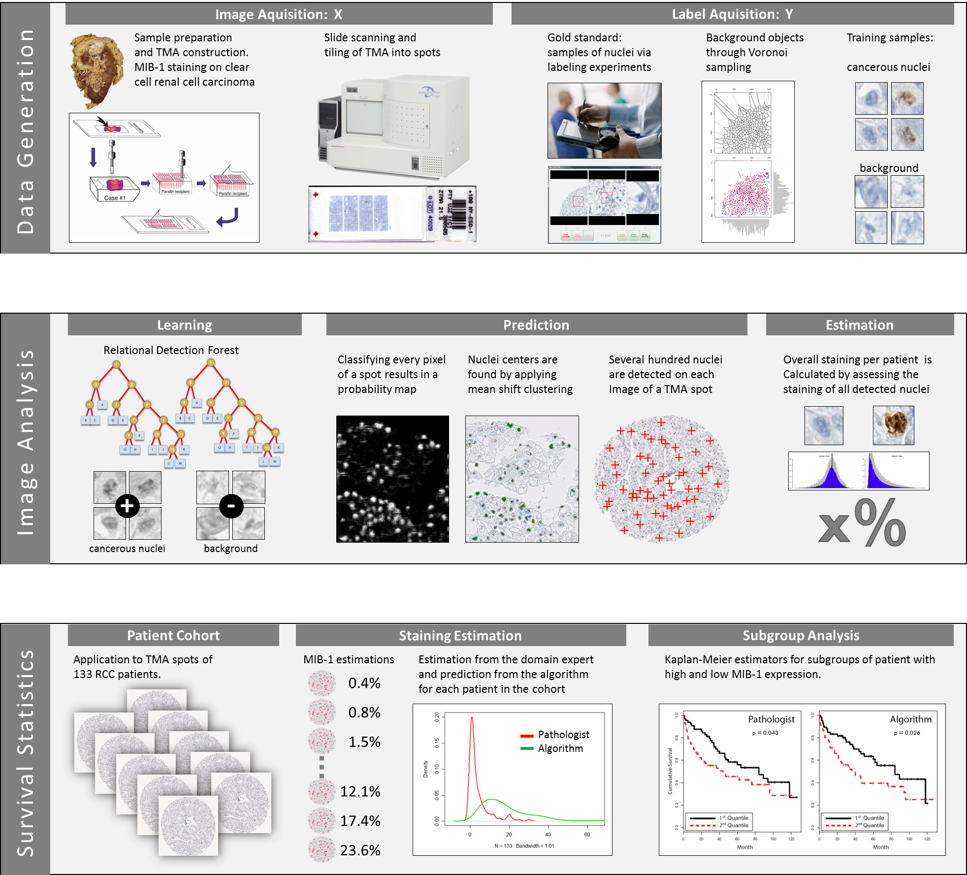
Figure 8 depicts a schematic overview of the project subdivided into the three main parts which are discussed in the following:
5.1 Data Generation
The data generation process consists of acquiring images of the TMA spots representing the covariates in the statistical model and the target variable which comprises detection and classification labels for nuclei.
The tissue microarray block was generated in a trial at the University Hospital Zurich. TMA slides were immunohistochemically stained with the MIB-1 (Ki-67) antigen and scanned on a Nanozoomer C9600 virtual slide light microscope scanner from HAMAMATSU. The magnification of resulted in a per pixel resolution of . The tissue microarry was tiled into single spots of size pixel, representing one patient each.
Various strategies can be devised to estimate the progression status of cancerous tissue: (i) we could first detect cell nuclei and then classify the detected nuclei as cancerous or benign [38]; (ii) the nucleus detection phase could be merged with the malignant/benign classification to simultaneously train a sliding window detector for cancerous nuclei only. To this end samples of cancerous nuclei were collected using the labeling experiments described in Section 2.3. Voronoi Sampling [42] was used to generate a set of negative background patches which are spatially well distributed in the training images. Hence a Voronoi tessellation is created based on the locations of the positive samples and background patches are sampled at the vertices of the Voronoi diagram. In contrast to uniform rejection sampling, using a tessellation has the advantage that the negative samples are concentrated on the area of tissue close to the nulei and few samples are spent on the homogeneous background. (The algorithm should not be confused with Lloyd’s algorithm [101] which is also known as Voronoi iteration.) The result of the data generation process is a labeled set of image patches of size pixel.
5.2 Image Analysis
The image analysis part of the pipeline consists of learning a relational detection forest [42] based on the samples extracted in the previous step. To guarantee illumination invariance, the feature basis described in Section 3.1 is used.
The strong class imbalance in the training set is accounted for by randomly subsampling the background class for each tree of the ensemble. The model parameters are adjusted by optimizing the out of bag (OOB) error [43] and they consist of the number of trees, the maximum tree depth and the number of features sampled at each node in a tree.
For prediction each pixel of a TMA spot is classified by the relation detection forest. This results in a probability map in the size of the image where the gray value at each position indicates the probability of being the location of a cancerous nucleus. Finally, weighted mean shift clustering is conducted with a circular box kernel based on the average radius of the nuclei in the training set. This process yields the final coordinates of the detected cancerous nuclei.
To differentiate a stained nucleus from a non-stained nucleus a simple color model is learned. Based on the labeled nuclei, color histograms are generated for both classes based on the pixels within a radius . A test nucleus is then classified based on the distance to the centroid histograms of both classes.
The final staining estimation per patient is achieved by calculating the percentage of stained cancerous nuclei.
5.3 Survival Statistics
The only objective endpoint in the majority of TMA studies is the prediction of the number of months a patient survived. The experiments described in Section 2.3 document the large disagreement between pathologists for the estimation of staining. Hence, fitting an algorithm to the estimates of a single pathologist or to a consensus voting of a commitee of pathologist is not desirable.
To this end the proposed computational pathology framework is validated against the right censored clinical survival data of the ccRCC patients. In addition these results were compared to the estimations of an expert pathologist specialized on renal cell carcinoma. He analyzed all spots in an exceptional thorough manner which required him more than two hours. This time consuming annotation exceeds the standard clinical practice significantly by a factor of and, therefore, the results can be viewed as an excellent human estimate for this dataset.
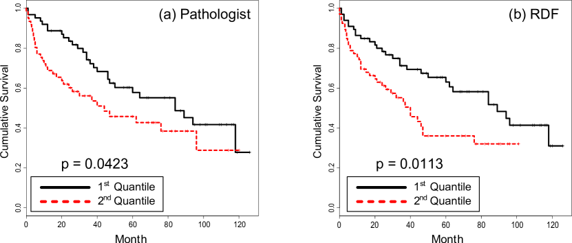
Figure 9 shows Kaplan-Meier plots of the estimated cumulative survival for the pathologist and the computational pathology framework. The farther the survival estimates of the two groups are separated the better the estimation. Quantifying this difference with a log-rank test shows that the proposed framework performs favorable () to the trained pathologist () and it can differentiate between the survival expectancy of the two groups of patients.
5.4 Project Conclusion
The presented computational pathology framework can be characterized by the following properties: (i) Simplicity: It can be used in a plug-and-play fashion to train object detectors in near real time for large variety of tasks. (ii) Novel Feature Basis: The introduced relational features are able to capture shape information, they are illumination invariant and extremely fast to evaluate. (iii) Randomization: The randomized tree induction algorithm is able to exploit the richness of the intractable large feature space and to take advantage of it by increasing diversity of the ensemble. (iv) Real World Applicability: The proposed algorithms perform well not only on renal cancer tissue but also in fluorescent imaging of pancreatic islets [78] and in quantifying staining in murine samples [102].
6 Future Directions
6.1 Histopathological Imaging
One promising research direction in medical image analysis points to online learning and interactive learning of computer vision models. Not only covers histopathology a broad and heterogeneous field but new biomarkers, antibodies and stainings are developed on a daily basis. To this end, real world applications have to quickly adapt to changing tissue types and staining modalities. Domain experts should be able to train these models in an interactive fashion to accustom novel data. For example, a classifier for object detection can be trained by clicking on novel objects or correcting for false detections.
A necessary prerequisite for research in computational pathology proved to be the scanning of whole slides and TMAs. [103] describe a fully digital pathology slide archive which has been assembled by high-volume tissue slide scanning. The Peta bytes of histological data which will be available in the near future pose also a number of software engineering challenges, including distributed processing of whole slides and TMAs in clusters or the cloud, multiprocessor and multicore implementations of analysis algorithms and facilitating real time image processing on GPUs.
6.2 Clinical Application and Decision Support
In today’s patient care we observe the interesting trend to integrate pathological diagnoses in web based patient files. Avatar based visualization proved to be useful not only for medical experts but also for a new generation of patients who are better informed and demand online updated and appropriately visualized informations about their own disease state and treatment procedures.
Furthermore this approach can be extended for decision support by statistical models which are able to utilize this unified view of patients incorporating data from a large variety of clinical sources, e.g. pathology, cytology, radiology, etc.
6.3 Pathology@home
Real-time, in vivo cancer detection on cellular level appears as a futuristic dream in patient care but could be a reality in a few years. [104] constructed a fiber-optic fluorescence microscope using a consumer-grade camera for in vivo cellular imaging. The fiber-optic fluorescence microscope includes an LED light, an objective lens, a fiber-optic bundle, and a consumer-grade DSLR. The system was used to image an oral cancer cell line, a human tissue specimen and the oral mucosa of a healthy human subject in vivo, following topical application of proflavine. The fiber-optic microscope resolved individual nuclei in all specimens and tissues imaged. This capability allowed qualitative and quantitative differences between normal and precancerous or cancerous tissues to be identified. In combination with a computational pathology framework, this technique would allow the real time classification of cancerous cells in epithelial tissues. Such a portable and inexpensive system is especially interesting for patient care in low-resource settings like the developing world.
Constructing a microscope for mobile phones defines the future of patient care in remote sites with centralized analysis support. [105] built a mobile phone-mounted light microscope and demonstrated its potential for clinical use by imaging sickle and P. falciparum-infected red blood cells in brightfield and M. tuberculosis-infected sputum samples in fluorescence with LED excitation. In all cases the resolution exceeded the critical level that is necessary to detect blood cell and microorganism morphology. This concept could provide an interesting tool for disease diagnosis and screening, especially in the developing world and rural areas where laboratory facilities are scarce but mobile phone infrastructure is available.
6.4 Standards and Exchange Formats
One of the major obstacles for wide spread use of computational pathology is the absence of generally agreed upon standards and exchange formats. This deficit not only handicaps slide processing management and whole slide digital imaging [106], but it also extends to statistical models and analysis software. Standardized exchange formats would support project specific combinations of object detectors, staining estimation algorithms and medical statistics. It would be very much desirable if at least the research community would agree on a few simple interfaces for data and model exchange.
6.5 Further Reading
All links and references presented in this review together with software, statistical models and a blog about the topic are available from www.computational-pathology.org.
Acknowledgments
The authors wish to thank Holger Moch and Peter Schraml for their help in conducting the RCC TMA project, Peter Wild and Peter Bode for annotating the medical data and Monika Bieri and Norbert Wey for scanning and tiling the TMA slides. Special thanks also to Volker Roth and Sudhir Raman for valuable discussions. We also acknowledge financial support from the FET program within the EU FP7, under the SIMBAD project (Contract 213250).
References
- [1] D. Grignon, J. Eble, S. Bonsib, H. Moch, Clear cell renal cell carcinoma, World Health Organization Classification of Tumours. Pathology and Genetics of Tumours of the Urinary System and Male Genital Organs. IARC Press.
- [2] A. Tannapfel, H. Hahn, A. Katalinic, R. Fietkau, R. Kuehn, C. Wittekind, Prognostic value of ploidy and proliferation markers in renal cell carcinoma., Cancer Jan 1;77(1) (1996) 164–71.
- [3] e. a. Moch H, Schraml P, High-throughput tissue microarray analysis to evaluate genes uncovered by cdna microarray screening in renal cell carcinoma., Am J Pathol. Apr;154(4) (1999) 981–6.
- [4] L. W. Sudarshan S, Genetic basis of cancer of the kidney, Semin Oncol. Oct;33(5) (2006) 544–51.
- [5] e. a. Nocito A, Bubendorf L, Microarrays of bladder cancer tissue are highly representative of proliferation index and histological grade., J Pathol. Jul;194(3): (2001) 349–57.
- [6] H. Moch, W. Artibani, B. Delahunt, V. Ficarra, R. Knuechel, F. Montorsi, J.-J. Patard, C. G. Stief, T. Sulser, P. J. Wild, Reassessing the current uicc/ajcc tnm staging for renal cell carcinoma, European Urology 56 (4) (2009) 636 – 643.
- [7] J. Kononen, L. Bubendorf, A. Kallionimeni, M. Barlund, P. Schraml, S. Leighton, J. Torhorst, M. J. Mihatsch, G. Sauter, O.-P. Kallionimeni, Tissue microarrays for high-throughput molecular profiling of tumor specimens, Nat Med 4 (7) (1998) 844–847.
- [8] e. a. Takahashi M, Rhodes DR, Gene expression profiling of clear cell renal cell carcinoma: gene identification and prognostic classification., in: Proc Natl Acad Sci U S A., Vol. Aug 14;98(17), 2001, pp. 9754–9.
- [9] e. a. Young AN, Amin MB, Expression profiling of renal epithelial neoplasms: a method for tumor classification and discovery of diagnostic molecular markers., Am J Pathol. May;158(5) (2001) 1639–51.
- [10] S. C. Saur, H. Alkadhi, L. Desbiolles, T. J. Fuchs, G. Szekely, P. C. Cattin, Guided review by frequent itemset mining: additional evidence for plaque detection., Int J Comput Assist Radiol Surg 4 (3) (2009) 263–271.
- [11] S. C. Saur, H. Alkadhi, P. Stolzmann, S. Baumueller, S. Leschka, H. Scheffel, L. Desbiolles, T. J. Fuchs, G. Szekely, P. C. Cattin, Effect of reader experience on variability, evaluation time and accuracy of coronary plaque detection with computed tomography coronary angiography., Eur Radiol 20 (7) (2010) 1599–1606.
- [12] T. W. Nattkemper, T. Twellmann, H. Ritter, W. Schubert, Human vs. machine: evaluation of fluorescence micrographs, Computers in Biology and Medicine 33 (1) (2003) 31 – 43.
- [13] P. Welinder, P. Perona, Online crowdsourcing: rating annotators and obtaining cost-effective labels, in: Workshop on Advancing Computer Vision with Humans in the Loop at CVPR’10, 2010.
- [14] J. N. Eble, G. Sauter, J. I. Epstein, I. A. Sesterhenn, Pathology and Genetics of Tumours of the Urinary System and Male Genital Organs, Vol. 7 of Classification of Tumours, World Health Organization, 2004.
- [15] P. Smyth, U. M. Fayyad, M. C. Burl, P. Perona, P. Baldi, Inferring ground truth from subjective labelling of venus images, in: NIPS, 1994, pp. 1085–1092.
- [16] V. C. Raykar, S. Yu, L. H. Zhao, A. Jerebko, C. Florin, G. H. Valadez, L. Bogoni, L. Moy, Supervised learning from multiple experts: whom to trust when everyone lies a bit, in: ICML ’09: Proceedings of the 26th Annual International Conference on Machine Learning, ACM, New York, NY, USA, 2009, pp. 889–896.
- [17] J. Whitehill, P. Ruvolo, T. fan Wu, J. Bergsma, J. Movellan, Whose vote should count more: Optimal integration of labels from labelers of unknown expertise, in: Y. Bengio, D. Schuurmans, J. Lafferty, C. K. I. Williams, A. Culotta (Eds.), Advances in Neural Information Processing Systems 22, 2009, pp. 2035–2043.
- [18] T. Kauppi, J.-K. Kamarainen, L. Lensu, V. Kalesnykiene, I. Sorri, H. Kälviäinen, H. Uusitalo, J. Pietilä, Fusion of multiple expert annotations and overall score selection for medical image diagnosis, in: SCIA ’09: Proceedings of the 16th Scandinavian Conference on Image Analysis, Springer-Verlag, Berlin, Heidelberg, 2009, pp. 760–769.
- [19] G. Lugosi, Learning with an unreliable teacher, Pattern Recogn. 25 (1) (1992) 79–87.
- [20] P. Smyth, Bounds on the mean classification error rate of multiple experts, Pattern Recognition Letters 17 (12) (1996) 1253 – 1257.
- [21] O. Dekel, O. Shamir, Vox populi: Collecting high-quality labels from a crowd, in: Proceedings of the 22nd Annual Conference on Learning Theory (COLT 2009), 2009.
- [22] G. Tullock, Problems of majority voting, The Journal of Political Economy 67 (6) (1959) 571–579.
- [23] A. Downs, Problems of majority voting: In defense of majority voting, The Journal of Political Economy 69 (2) (1961) 192–199.
-
[24]
A. Frank, A. Asuncion, UCI machine
learning repository (2010).
URL http://archive.ics.uci.edu/ml - [25] L. Berglund, E. Bjoerling, P. Oksvold, L. Fagerberg, A. Asplund, C. Al-Khalili Szigyarto, A. Persson, J. Ottosson, H. Wernerus, P. Nilsson, E. Lundberg, A. Sivertsson, S. Navani, K. Wester, C. Kampf, S. Hober, F. Ponten, M. Uhlen, A Genecentric Human Protein Atlas for Expression Profiles Based on Antibodies, Molecular & Cellular Proteomics 7 (10) (2008) 2019–2027.
- [26] F. Pontén, K. Jirström, M. Uhlen, The human protein atlas – a tool for pathology, The Journal of Pathology 216 (4) (2008) 387–393.
- [27] E. Drelie Gelasca, B. Obara, D. Fedorov, K. Kvilekval, B. Manjunath, A biosegmentation benchmark for evaluation of bioimage analysis methods, BMC Bioinformatics 10 (1) (2009) 368.
- [28] O. Lezoray, H. Cardot, Cooperation of color pixel classification schemes and color watershed: a study for microscopical images, IEEE transactions on Image Processing 11 (7) (2002) 783–789.
- [29] C. Meurie, O. Lezoray, C. Charrier, A. Elmoataz, Combination of multiple pixel classifiers for microscopic image segmentation, IJRA (IASTED International Journal of Robotics and Automation) 20 (2) (2005) 63–69, special issue on Colour Image Processing and Analysis for Machine Vision, ISSN 0826-8185.
- [30] O. Lezoray, A. Elmoataz, H. Cardot, A color object recognition scheme: application to cellular sorting, Machine Vision and Applications 14 (2003) 166–171.
- [31] L. P. Coelho, A. Shariff, R. F. Murphy, Nuclear segmentation in microscope cell images: a hand-segmented dataset and comparison of algorithms, in: ISBI’09: Proceedings of the Sixth IEEE international conference on Symposium on Biomedical Imaging, IEEE Press, Piscataway, NJ, USA, 2009, pp. 518–521.
- [32] A. Lehmussola, P. Ruusuvuori, J. Selinummi, H. Huttunen, O. Yli-Harja, Computational framework for simulating fluorescence microscope images with cell populations, Medical Imaging, IEEE Transactions on 26 (7) (2007) 1010 –1016.
- [33] J. P. Monaco, J. E. Tomaszewski, M. D. Feldman, I. Hagemann, M. Moradi, P. Mousavi, A. Boag, C. Davidson, P. Abolmaesumi, A. Madabhushi, High-throughput detection of prostate cancer in histological sections using probabilistic pairwise markov models, Medical Image Analysis 14 (4) (2010) 617 – 629.
- [34] M. Gurcan, L. Boucheron, A. Can, A. Madabhushi, N. Rajpoot, B. Yener, Histopathological image analysis: A review, Biomedical Engineering, IEEE Reviews in 2 (2009) 147 –171.
- [35] M. Rojo, G. Bueno, J. Slodkowska, Review of imaging solutions for integrated quantitative immunohistochemis try in the pathology daily practice, Folia Histochemica et Cytobiologica 47 (3) (2009) 349–354.
- [36] P. Soille, Morphological Image Analysis: Principles and Applications, Springer-Verlag New York, Inc., Secaucus, NJ, USA, 2003.
- [37] Color image segmentation using morphological clustering and fusion with automatic scale selection, Pattern Recognition Letters 30 (4) (2009) 397 – 406.
- [38] T. J. Fuchs, T. Lange, P. J. Wild, H. Moch, J. M. Buhmann, Weakly supervised cell nuclei detection and segmentation on tissue microarrays of renal cell carcinoma, in: Pattern Recognition. DAGM 2008, Vol. 5096 of Lecture Notes in Computer Science, Springer Berlin / Heidelberg, 2008, pp. 173–182.
- [39] N. Halama, I. Zoernig, A. Spille, K. Westphal, P. Schirmacher, D. Jaeger, N. Grabe, Estimation of immune cell densities in immune cell conglomerates: An approach for high-throughput quantification, PLoS ONE 4 (11) (2009) e7847.
- [40] M. Arif, N. Rajpoot, Classification of potential nuclei in histology images using shape manifold learning, in: Proceedings International Conference on Machine Vision (ICMV’2007), 2007.
- [41] M. Macenko, M. Niethammer, J. S. Marron, D. Borland, J. T. Woosley, X. Guan, C. Schmitt, N. E. Thomas, A method for normalizing histology slides for quantitative analysis, in: ISBI’09: Proceedings of the Sixth IEEE international conference on Symposium on Biomedical Imaging, IEEE Press, Piscataway, NJ, USA, 2009, pp. 1107–1110.
- [42] T. J. Fuchs, J. Haybaeck, P. J. Wild, M. Heikenwalder, H. Moch, A. Aguzzi, J. M. Buhmann, Randomized tree ensembles for object detection in computational pathology., in: ISVC (1), Vol. 5875 of Lecture Notes in Computer Science, Springer, 2009, pp. 367–378.
- [43] L. Breiman, Random forests., Machine Learning 45 (1) (2001) 5–32.
- [44] D. Geman, C. d’Avignon, D. Q. Naiman, R. L. Winslow, Classifying gene expression profiles from pairwise mrna comparisons, Statistical Applications in Genetics and Molecular Biology 3 (1) (2004) 19.
- [45] P. Viola, M. Jones, Rapid object detection using a boosted cascade of simple features, in: Proceedings of the 2001 IEEE Computer Society Conference on Computer Vision and Pattern Recognition. CVPR 2001, Vol. 1, IEEE Comput. Soc, Los Alamitos, CA, USA, 2001, pp. I–511–I–518.
- [46] Y. Freund, R. Schapire, Experiments with a new boosting algorithm, Machine Learning: Proceedings of the Thirteenth International Conference (1996) 148–156.
- [47] P. Geurts, D. Ernst, L. Wehenkel, Extremely randomized trees, Machine Learning 63 (1) (2006) 3–42.
- [48] T. J. Fuchs, J. M. Buhmann, Inter-active learning of randomized tree ensembles for object detection, in: ICCV Workshop on On-line Learning for Computer Vision, 2009, IEEE, 2009.
- [49] V. Vapnik, Statistical Learning Theory, Wiley, New York, 1998, forthcoming.
- [50] A. Blum, On-line algorithms in machine learning, in: Online Algorithms, 1996, pp. 306–325.
- [51] T. T. Nguyen, H. Grabner, H. Bischof, B. Gruber, On-line boosting for car detection from aerial images., in: RIVF, IEEE, 2007, pp. 87–95.
- [52] H. Celik, A. Hanjalic, E. Hendriks, S. Boughorbel, Online training of object detectors from unlabeled surveillance video, in: Computer Vision and Pattern Recognition Workshops, 2008. CVPRW ’08. IEEE Computer Society Conference on, 2008, pp. 1–7.
- [53] H. Grabner, C. Leistner, H. Bischof, Semi-supervised on-line boosting for robust tracking, in: ECCV (1), 2008, pp. 234–247.
- [54] P. M. Roth, H. Grabner, C. Leistner, M. Winter, H. Bischof, Interactive learning a person detector: Fewer clicks - less frustration, in: Proc. Workshop of the Austrian Association for Pattern Recognition, 2008.
- [55] Y. Amit, D. G. Y, Shape quantization and recognition with randomized trees, Neural Computation 9 (1997) 1545–1588.
- [56] N. C. Oza, Online ensemble learning, Ph.D. thesis, The University of California, Berkeley, CA (Sep 2001).
- [57] A. Fern, R. Givan, Online ensemble learning: An empirical study, Machine Learning 53 (1-2) (2003) 71–109.
- [58] O. H. Elgawi, Online random forests based on corrfs and corrbe, in: Computer Vision and Pattern Recognition Workshops, 2008. CVPRW ’08. IEEE Computer Society Conference on, 2008, pp. 1–7.
- [59] P. E. Utgoff, Incremental induction of decision trees, Machine Learning 4 (1989) 161–186.
- [60] P. E. Utgoff, An improved algorithm for incremental induction of decision trees, in: ICML, 1994, pp. 318–325.
- [61] D. Kalles, T. Morris, Efficient incremental induction of decision trees, Machine Learning 24 (3) (1996) 231–242.
- [62] B. Pfahringer, G. Holmes, R. Kirkby, New options for hoeffding trees., in: M. A. Orgun, J. Thornton (Eds.), Australian Conference on Artificial Intelligence, Vol. 4830 of Lecture Notes in Computer Science, Springer, 2007, pp. 90–99.
- [63] N. Littlestone, Learning quickly when irrelevant attributes abound: A new linear-threshold algorithm, in: Machine Learning, 1988, pp. 285–318.
- [64] N. Littlestone, M. K. Warmuth, The weighted majority algorithm, in: FOCS, 1989, pp. 256–261.
- [65] F. Hayes-Roth, D. A. Waterman, D. B. Lenat, Building expert systems, Addison-Wesley Longman Publishing Co., Inc., Boston, MA, USA, 1983.
- [66] R. M. Levenson, J. R. Mansfield, Multispectral imaging in biology and medicine: Slices of life, Cytometry Part A 69A (8) (2006) 748–758.
- [67] C. M. van der Loos, Multiple immunoenzyme staining: Methods and visualizations for the observation with spectral imaging, J. Histochem. Cytochem. 56 (4) (2008) 313–328.
- [68] L. Boucheron, Z. Bi, N. Harvey, B. Manjunath, D. Rimm, Utility of multispectral imaging for nuclear classification of routine clinical histopathology imagery, BMC Cell Biology 8 (Suppl 1) (2007) S8.
- [69] W. J. Cukierski, X. Qi, D. J. Foran, Moving beyond color: the case for multispectral imaging in brightfield pathology, in: ISBI’09: Proceedings of the Sixth IEEE international conference on Symposium on Biomedical Imaging, IEEE Press, Piscataway, NJ, USA, 2009, pp. 1111–1114.
- [70] A. Rabinovich, S. Agarwal, C. A. Laris, J. H. Price, S. Belongie, Unsupervised color decomposition of histologically stained tissue samples, in: in Advances in Neural Information Processing Systems, MIT Press, 2003.
- [71] D. D. Lee, H. S. Seung, Learning the parts of objects by non-negative matrix factorization, Nature 401 (6755) (1999) 788–791.
- [72] A. Hyvarinen, Independent component analysis, Neural Computing Surveys 2.
- [73] A. C. Ruifrok, D. A. Johnston, Quantification of histochemical staining by color deconvolution (2001).
- [74] G. Begelman, M. Zibulevsky, E. Rivlin, T. Kolatt, Blind decomposition of transmission light microscopic hyperspectral cube using sparse representation, Medical Imaging, IEEE Transactions on 28 (8) (2009) 1317 –1324.
- [75] T. Zimmermann, 2005, Ch. Spectral Imaging and Linear Unmixing in Light Microscopy, pp. 245–265.
- [76] J. Y. Newberg, J. Li, A. Rao, F. Pontén, M. Uhlén, E. Lundberg, R. F. Murphy, Automated analysis of human protein atlas immunofluorescence images, in: ISBI’09: Proceedings of the Sixth IEEE international conference on Symposium on Biomedical Imaging, IEEE Press, Piscataway, NJ, USA, 2009, pp. 1023–1026.
- [77] J. Herold, L. Zhou, S. Abouna, S. Pelengaris, D. Epstein, M. Khan, T. W. Nattkemper, Integrating semantic annotation and information visualization for the analysis of multichannel fluorescence micrographs from pancreatic tissue, Computerized Medical Imaging and Graphics In Press, Corrected Proof (2009) –.
- [78] X. E. Floros, T. J. Fuchs, M. P. Rechsteiner, G. Spinas, H. Moch, J. M. Buhmann, Graph-based pancreatic islet segmentation for early type 2 diabetes mellitus on histopathological tissue, in: MICCAI (1), 2009, pp. 633–640.
- [79] A. Wetzel, Computational aspects of pathology image classification and retrieval, J. Supercomput. 11 (3) (1997) 279–293.
- [80] G. Thallinger, K. Baumgartner, M. Pirklbauer, M. Uray, E. Pauritsch, G. Mehes, C. Buck, K. Zatloukal, Z. Trajanoski, Tamee: data management and analysis for tissue microarrays, BMC Bioinformatics 8 (1) (2007) 81.
- [81] D. J. Foran, L. Yang, O. Tuzel, W. Chen, J. Hu, T. M. Kurc, R. Ferreira, J. H. Saltz, A cagrid-enabled, learning based image segmentation method for histopathology specimens, in: ISBI’09: Proceedings of the Sixth IEEE international conference on Symposium on Biomedical Imaging, IEEE Press, Piscataway, NJ, USA, 2009, pp. 1306–1309.
- [82] S. Oster, S. Langella, S. Hastings, D. Ervin, R. Madduri, J. Phillips, T. Kurc, F. Siebenlist, P. Covitz, K. Shanbhag, I. Foster, J. Saltz, caGrid 1.0: An Enterprise Grid Infrastructure for Biomedical Research, Journal of the American Medical Informatics Association 15 (2) (2008) 138–149.
- [83] E. L. Kaplan, P. Meier, Nonparametric estimation from incomplete observations, Journal of the American Statistical Association 53 (282) 457–481.
- [84] N. Mantel, W. Haenszel, Statistical aspects of the analysis of data from retrospective studies of disease, J Natl Cancer Inst 4 (22) (1959) 719–748.
- [85] J. P. Klein, M. L. Moeschberger, Survival Analysis: Techniques for Censored and Truncated Data, Springer-Verlag:New York Inc, 1997.
- [86] D. R. Cox, Regression models and life-tables, Journal of the Royal Statistical Society. Series B (Methodological) 34 (2) 187–220.
- [87] V. Roth, T. J. Fuchs, S. Raman, P. Wild, E. Dahl, J. M. Buhmann, Full bayesian survival models for analyzing human breast tumors, in: NIPS Workshop: MLCP–Machine Learning in Computational Biology, 2008.
- [88] D. S. Joseph G.Ibrahim, Ming-Hui Chen, Bayesian Survival Analysis, Springer-Verlag:New York Inc, 2001.
- [89] C. Dahinden, B. Ingold, P. Wild, G. Boysen, V.-D. Luu, M. Montani, G. Kristiansen, T. Sulser, P. Buehlmann, H. Moch, P. Schraml, Mining Tissue Microarray Data to Uncover Combinations of Biomarker Expression Patterns that Improve Intermediate Staging and Grading of Clear Cell Renal Cell Cancer, Clinical Cancer Research 16 (1) (2010) 88–98.
- [90] P. McCullaghand, J. Nelder, Generalized Linear Models, Chapman & Hall, 1983.
- [91] O. Rosen, M. Tanner, Mixtures of proportional hazards regression models, Statistics in Medicine 18 (1999) 1119–1131.
- [92] T. Ando, S. Imoto, S. Miyano, Kernel mixture survival models for identifying cancer subtypes, predicting patient’s cancer types and survival probabilities (2004).
- [93] A. Kottas, Nonparametric Bayesian survival analysis using mixtures of Weibull distributions, Journal of Statistical Planning and Inference 136 (3) (2006) 578 – 596.
- [94] J. G. Ibrahim, M. hui Chen, S. N. Maceachern, Bayesian variable selection for proportional hazards models (1996).
- [95] M. D. Paserman, Bayesian inference for duration data with unobserved and unknown heterogeneity: Monte carlo evidence and an application, Iza discussion papers, Institute for the Study of Labor (IZA) (Jan. 2004).
- [96] C. E. Rasmussen, Z. Ghahramani, Infinite mixtures of gaussian process experts, in: In Advances in Neural Information Processing Systems 14, MIT Press, 2001, pp. 881–888.
- [97] S. Raman, T. J. Fuchs, P. J. Wild, E. Dahl, V. Roth, The bayesian group-lasso for analyzing contingency tables, in: ICML ’09: Proceedings of the 26th Annual International Conference on Machine Learning, ACM, New York, NY, USA, 2009, pp. 881–888.
- [98] S. Raman, V. Roth, Sparse bayesian regression for grouped variables in generalized linear models, in: Proceedings of the 31st DAGM Symposium on Pattern Recognition, 2009, pp. 242–251.
- [99] M. Yuan, Y. Lin, Model selection and estimation in regression with grouped variables, J. Roy. Stat. Soc. B (2006) 49–67.
- [100] T. J. Fuchs, P. J. Wild, H. Moch, J. M. Buhmann, Computational pathology analysis of tissue microarrays predicts survival of renal clear cell carcinoma patients, in: Medical Image Computing and Computer-Assisted Intervention. MICCAI 2008, Vol. 5242 of Lecture Notes in Computer Science, Springer Berlin / Heidelberg, 2008, pp. 1–8.
- [101] S. P. Lloyd, Least squares quantization in pcm, Information Theory, IEEE Transactions on 28 (2) (1982) 129–137.
- [102] K. Bettermann, M. Vucur, J. Haybaeck, C. Koppe, J. Janssen, F. Heymann, A. Weber, R. Weiskirchen, C. Liedtke, N. Gassler, M. Mueller, R. de Vos, M. J. Wolf, Y. Boege, G. M. Seleznik, N. Zeller, D. Erny, T. Fuchs, S. Zoller, S. Cairo, M.-A. Buendia, M. Prinz, S. Akira, F. Tacke, M. Heikenwalder, C. Trautwein, T. Luedde, Tak1 suppresses a nemo-dependent but nf-[kappa]b-independent pathway to liver cancer, Cancer Cell 17 (5) (2010) 481 – 496.
- [103] A. Huisman, A. Looijen, S. M. van den Brink, P. J. van Diest, Creation of a fully digital pathology slide archive by high-volume tissue slide scanning, Human Pathology 41 (5) (2010) 751 – 757.
- [104] D. Shin, M. C. Pierce, A. M. Gillenwater, M. D. Williams, R. R. Richards-Kortum, A fiber-optic fluorescence microscope using a consumer-grade digital camera for ¡italic¿in vivo¡/italic¿ cellular imaging, PLoS ONE 5 (6) (2010) e11218.
- [105] D. N. Breslauer, R. N. Maamari, N. A. Switz, W. A. Lam, D. A. Fletcher, Mobile phone based clinical microscopy for global health applications, PLoS ONE 4 (7) (2009) e6320.
- [106] C. Daniel, M. Garc?a Rojo, K. Bourquard, D. Henin, T. Schrader, V. D. Mea, J. Gilbertson, B. A. Beckwith, Standards to support information systems integration in anatomic pathology, Archives of Pathology & Laboratory Medicine 133 (11) (2009) 1841–1849.