Finite-size effects and switching times for Moran dynamics with mutation

Abstract

We consider the Moran process with two populations competing under an iterated Prisoners’ Dilemma in the presence of mutation, and concentrate on the case where there are multiple Evolutionarily Stable Strategies. We perform a complete bifurcation analysis of the deterministic system which arises in the infinite population size. We also study the Master equation and obtain asymptotics for the invariant distribution and metastable switching times for the stochastic process in the case of large but finite population. We also show that the stochastic system has asymmetries in the form of a skew for parameter values where the deterministic limit is symmetric.

1 Introduction

The mathematical study of models for evolution has a long history. The early work of Wright, Fisher, Moran, and Feller [Wri31, Fel51, Fis30, Mor58], where those authors studied of small population size on a model of neutral evolution (see [Cro10] for a nice overview of the early history of these studies). In parallel, the mathematical framework of game theory [vNM53] and evolutionary game theory [Smi82] has been used since to model and understand complexity in problems in evolution and ecology. A truly large volume of work has been developed in the last few decades using this approach [ML75, AH81, Axe84, NM92, Now06a, Axe97, Now06b, NS92, NS05, TFSN04, Wei97].

Most of the models mentioned above can be formulated as a Markov chain on a lattice, where the discrete points on the lattice correspond to integer sizes of the various subpopulations. In the limit of large population, this Markov chain undergoes smaller jumps (on the population scale), if this is coupled with an appropriate rescaling in time, we might expect a sensible limit to a continuum model. What is true is that if one does this rescaling properly, then in the limit of infinite population, the system does converge to an ODE. In the case of large but finite populations, the system is still stochastic, so it is of interest to study the invariant distributions of such a system, the rate and type of convergence to this equilibrium, and in particular switching processes between multiple equilibria. The first rigorous results in this direction were due to the pioneering work of Kurtz in the context of biochemical models [Kur72, Kur78], but have been followed up by a large number of analytic and numerical studies [Bre14, Bre10, VK92, VK82, DN08, Gar04, SW95, GG08].

The purpose of this paper is to apply the modern techniques of stochastic analysis to a particular model of evolutionary game theory. The model we consider is a version of a model described in [Now06a]; we consider a population consisting of organisms who can each play one of two strategies where the payoff matrix is of Prisoner’s Dilemma type, and the organisms evolve according to Moran dynamics, i.e. in each round of play, one organism is chosen to reproduce based on its fitness and one organism is killed at random, so that the population size remains constant. We also allow a positive probability for a mutation, i.e. there is a positive probability $\mu>0$ that an organism’s offspring is of the other type. We stress here that we consider a fully stochastic version of this model where all events are governed by a Markov process.

The infinite-population limit of this process (an ODE) is described in [Now06a], and it is shown there that for certain parameters the ODE supports two stable fixed points with disjoint basins of attraction, i.e. is multistable. We show that our Markov chain model limits on this ODE model as the population tends to infinity.

For population large but finite, however, the system is still noisy and can jump between the multiple attractors, although it will only do so on long timescales. Studying the timescale on which this jumping occurs is one of the main goals of this paper, and we give two different asymptotic descriptions of this timescale. Another interesting effect we show by considering the stochastic system (as compared to its deterministic limit) is we show that certain parameters that are indistinguishable in the limit give rise to biases for large but finite populations. For example, if we assume that the aggregate payoff is the same for both strategies (i.e. the sum of the payoffs against both friends and enemies is the same for both strategies), but one strategy plays better against enemies than it does against its friends, it will have an advantage for finite size populations, while being indistinguishable in the limit.

2 Model

2.1 Definition

In this paper, we consider a finite population of size $N$ consisting of two strategies, $A$ and $B$. We assume that payoffs from each individual game are awarded by a payoff matrix given by

$$\left[\begin{array}[]{c|cc}&A&B\\ \hline\cr A&a&b\\ B&c&d\end{array}\right].$$ (2.1)

Here, we represent the payoff to player1 in an interaction where player1’s play is along the left column, and player2’s play is on the top row. We assume that the payoff to player2 is always the transpose of this matrix. For example, when we have two players playing strategy $A$, they each receive a payoff of $a$, and if they both are strategy $B$, they each receive $d$. If two individuals with different strategies meet, if player1 is type $B$, player1 receives a payoff of $c$ while player2 receives a payoff of $b$.

Once the average payoffs are determined, each strategy is awarded a fitness value. Fitness can have many interpretations such as physical fitness or ability to collect food, but ultimately it affects the survival of individuals, and here we assume that the fitness is proportional to the payoff an individual receives playing the game. Specifically, if we assume that there are $i$ individuals of type $A$ in the population, then the function

$$f_{A}=\frac{ai+b(N-i)}{N},\quad\mbox{resp.}\quad f_{B}=\frac{ci+d(N-i)}{N},$$ (2.2)

represents the average fitness of an individual of type $A$ (resp. type $B$). This represents the average payoff an organism would receive if it chose an opponent at random and played the game described above.

We want to consider only evolutionarily stable strategies (ESS), those strategies which are resistant to invasion by a single mutant. For example, strategy $A$ will be ESS if $f_{A}>f_{B}$ when $i=N-1$ (i.e. when all but one organism is type $A$). This means that

$$a\frac{N-1}{N}+\frac{b}{N}>c\frac{N-1}{N}+\frac{d}{N},$$

and if we want this equation to hold for arbitrarily large populations, then the condition is clearly $a>c$. Similarly, strategy $B$ is ESS iff $d>b$. We will assume this in all that follows below.

After the fitness of each strategy is determined, the population evolves similar to a Moran Model, but with the possibility of a mutation during birth. In each round, one individual is chosen for reproduction with probability proportional to its fitness and gives birth to one offspring. However, this offspring is of the opposite type with probability $\mu\in(0,1)$. At each stage, one organism is chosen at random to be removed.

From this, we can view the model as a Markov process $\{X(t)_{t\geq 0}\}$ on the discrete state space $i=0,1,\cdots,N$ with transition rates

$$\omega_{+}(i;\mu) =\bigg{(}\frac{if_{A}}{if_{A}+(N-i)f_{B}}\bigg{)}\bigg{(}\frac{N-i}{N}\bigg{)}(1-\mu)+\bigg{(}\frac{(N-i)f_{B}}{if_{A}+(N-i)f_{B}}\bigg{)}\bigg{(}\frac{N-i}{N}\bigg{)}\mu$$ (2.3)

$$\omega_{-}(i;\mu) =\bigg{(}\frac{(N-i)f_{B}}{if_{A}+(N-i)f_{B}}\bigg{)}\bigg{(}\frac{i}{N}\bigg{)}(1-\mu)+\bigg{(}\frac{if_{A}}{if_{A}+(N-i)f_{B}}\bigg{)}\bigg{(}\frac{i}{N}\bigg{)}\mu.$$ (2.4)

Here the state represents the number of organisms of type $A$. To see these rates, note that to have the transition $i\mapsto i+1$, either an individual with strategy $A$ needs to reproduce (with no mutation) and an individual with strategy $B$ needs to die, or an individual with strategy $B$ needs to reproduce (with mutation) and an individual with strategy $B$ needs to die. Similar arguments can be made for moving from state $i$ to $i-1$. (Of course, these rates do not add to one, since there is a possibility that the population size does not change: for example, if an individual of type $A$ reproduces without mutation, but an individual of type $A$ is also selected to die, then there is no change in the population, etc.)

Throughout this paper we will often switch between the extensive variable $i$ and the scaled variable $x=\frac{i}{N}$. In the limit as $N\rightarrow\infty$, we treat $x$ as a continuous variable. It is also assumed that the transition rates obey the scaling law $\omega_{\pm}(i;\mu)=N\Omega_{\pm}(x;\mu)$.

The following sections study this process both deterministically and stochastically. For given parameters $a$, $b$, $c$, $d$, and $\mu$ we seek to describe the distribution of strategies within the population and determine which strategy (if any) has an advantage.

We also remark that while the definition above seems to average out some of the randomness before we write down the Markov chain (e.g. we consider “average fitness” when writing down the transition rates in the chain), we could obtain the same model without such averaging. For example, if we assume that, at each timestep, each individual is paired with another individual in the population (selected with replacement) and then receives a deterministic payoff from (2.1), and then we choose individuals to reproduce with a probability proportional to their fitness, then again we would obtain (2.3, 2.4).

2.2 Parameter regimes

The results fall into three cases which arise naturally from the payoff matrix (2.1). Due to symmetry, we discuss only case 1.1 and case 2.

• Case 1 — $a+b=c+d$
  When populations $A$ and $B$ have equal size, $A$ and $B$ have equal fitness. There are three additional subcases.

  • Case 1.1 — $a>d$ and $b<c$
    $A$ has better self-interactions than strategy $B$, but strategy $B$ has better opponent interactions than strategy $A$.

  • Case 1.2 — $a<d$ and $b>c$
    Same as 1.1, but with the roles of $A$ and $B$ switched

  • Case 1.3 — $a=d$ and $b=c$
    Degenerate case where $A$ and $B$ are interchangable

• Case 2 — $a+b>c+d$
  When populations $A$ and $B$ have equal sizes, $A$ has a higher fitness than $B$.

• Case 3 — $a+b<c+d$
  When populations $A$ and $B$ have equal sizes, $B$ has a higher fitness than $A$.

For case 2, it is clear that strategy $A$ will have the advantage based on the asymmetry of the payoff matrix (2.1), and similarly for Case 3. Case 1.1 is not at all clear a priori. One could argue that strategy $A$ has the advantage because it has better self-interactions than strategy $B$, or that strategy $B$ has the advantage because it has better interaction with strategy $A$ than strategy $A$ has with strategy $B$. We will consider these more fully below.

2.3 Simulation Results

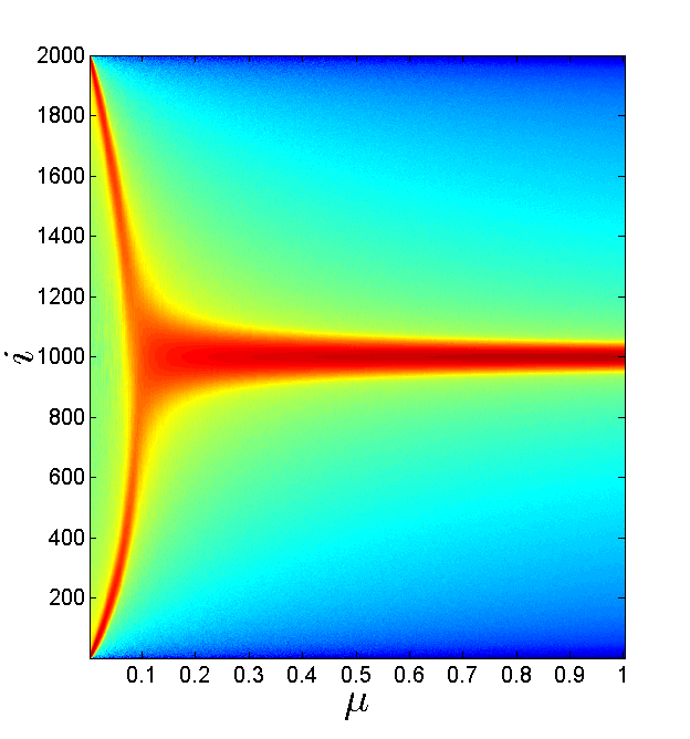
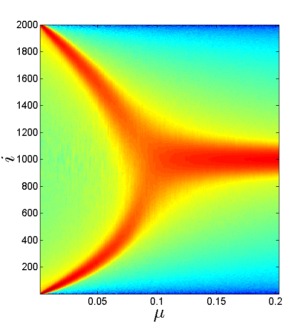
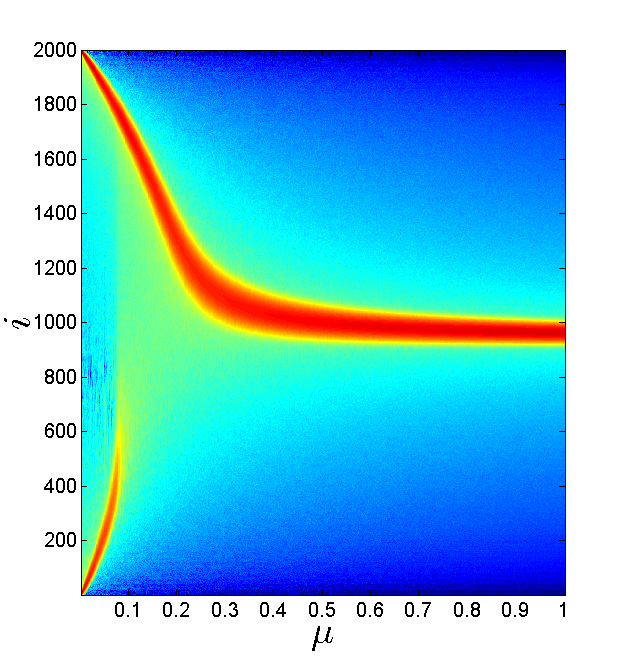
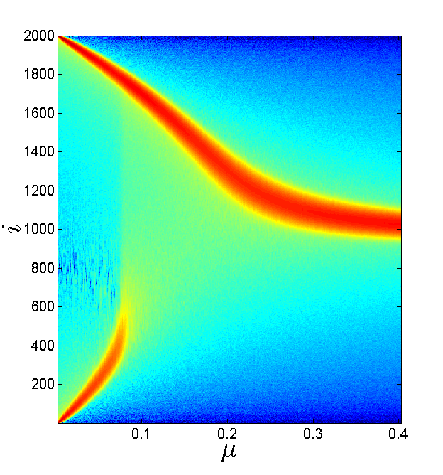
In Figures 1 and 2 we plot the invariant measure of the the Markov process (in fact, we are plotting the logarithm of this invariant measure for better contrast). Figure 1 corresponds to an example of case 1.1 and Figure 2 is an example of case 2.

The simulations were run for $200,000$ iterations with a burn in of $20,000$ and averaged over $100$ realizations. The colors towards the beginning of the rainbow represent densities closer to 1, while the lower colors represent densities closer to 0.

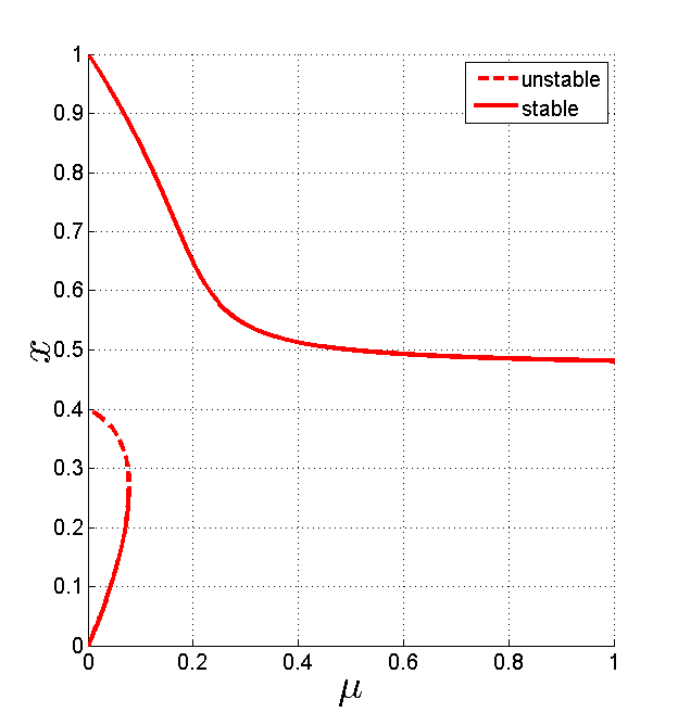
It is apparent from these pictures that when mutation is rare enough, there are two metastable mixtures that correspond to the fact that both strategies are ESS in the absence of mutation. As the mutation probability increases, these mixtures approach each other. In Figure 1, they seem to merge smoothly into a single stable mixture, whereas in Figure 2 one mixture disappears suddenly and the other takes over. We point out that these mixtures are metastable since we expect switching between them due to stochastic effects.

Figure 1: Monte Carlo simulation of the invariant distribution of the Markov process with $N=2000$. Both frames have parameters $a=4,b=1,c=3,d=2$; the right frame is a blowup of the left.

Figure 2: Monte Carlo simulation of the invariant distribution of the Markov process with $N=2000$. Both frames have parameters $a=4,b=2,c=1,d=4$; the right frame is a blowup of the left.

2.4 Connection to Prisoner’s Dilemma dynamics

Above, we have presented the payoff matrix (2.1) without any derivation. Here we discuss a bit about how such a matrix can arise. A common game-theoretic model to consider is that of the Prisoner’s Dilemma (PD), namely a payoff matrix

$$\left[\begin{array}[]{c|cc}&C&D\\ \hline\cr C&r&s\\ D&t&p\end{array}\right],$$ (2.5)

where $t>r>p>s$, and we use the same convention of symmetry as above, i.e. that player2’s payoff matrix is the transpose of player1’s. Each player has the option to “cooperate” or to “defect”. It is clear that if we assume the strategies are deterministic, the Nash equilibrium strategy is for both players to defect, since the second row is componentwise larger than the first. This is considered a dilemma because $r>p$, so that if the players could somehow agree to cooperate and trust each other, they would each receive a higher payoff, but in any situation where there is a lack of trust they are better off both defecting.

Now, we first note that the Prisoner’s Dilemma is not in the form mentioned above, since for us to have two strategies that are both ESS, we would need that $r>t$ to make $C$ stable. However, let us assume that the payoff matrix (2.1) is the aggregate payoff of an $m$-round game between two strategies that cooperate and defect in some pattern, is it possible to have both strategies be ESS?

The simplest case is if we assume that each strategy is to play $C$ and $D$ with some fixed probabilities, independent of the history of one’s opponent. For example, if we assume that strategy $A$ is to cooperate with probability $\alpha\in[0,1]$ and defect with probability $(1-\alpha)$, and similarly for strategy $B$ with probability $\beta$, then after a large algebraic computation we find that ${\mathrm{sign}}(a-c)={\mathrm{sign}}(\beta-\alpha)$ and ${\mathrm{sign}}(d-b)={\mathrm{sign}}(\alpha-\beta)$, and clearly it is not possible that both of these be positive. In particular, a strategy is ESS iff it is more likely to defect than the opposing strategy.

However, it is possible to construct strategies based on aggregate PD that allow for memory effects that give multiple ESS. For example, consider two strategies known as “tit-for-tat” (TFT) and “always defect” (AllD). In the former, the strategy is to cooperate in the first round, then do whatever the opponent did in the previous round; the second strategy is to always defect. If we assume that strategy $A$ is TFT and $B$ is AllD, then after $m$ rounds of play, the aggregate payoffs are

$$\left[\begin{array}[]{c|cc}&A&B\\ \hline\cr A&mr&s+(m-1)p\\ B&t+(m-1)p&mp\end{array}\right].$$ (2.6)

To see this, note that two players of type $A$ will always cooperate and two of type $B$ will always defect. If TFT plays AllD, then the first player will cooperate once and then defect forever, so will receive one payoff of $s$ and $m-1$ payoffs of $p$, while the second player will receive one payoff of $t$ and $m-1$ payoffs of $p$. Since $p>s$, we see that $B$ is ESS, but for $A$ to be ESS, we need $mr>t+(m-1)p$. But notice that $r>p$, so clearly for $m$ sufficiently large, $A$ is also ESS.

The types of mixtures that give rise to multiple ESS in a two-population game have a long history and have been studied extensively, see [ML75, Now06a, IFN07, WLCH08, ATG12].

3 Deterministic Bifurcation Analysis

The expected step size of the Markov process is given by

$$\frac{d\mathbb{E}[X(t)]}{dt}=\omega_{+}(X_{t};\mu)-\omega_{-}(X_{t};\mu),$$

where $\omega_{\pm}$ is defined in (2.3,2.4). Switching to the scaled variables and rates

$$x(t)=X_{t}/N\quad\omega_{\pm}(X_{t};\mu)=N\Omega_{\pm}(X_{t}/N;\mu),$$

we see that the deterministic equation

$$\frac{dx}{dt}=f(x;\mu):=\Omega_{+}(x;\mu)-\Omega_{-}(x;\mu)$$ (3.1)

describes the mean of the Markov process. As it turns out, in the limit $N\to\infty$, (3.1) also gives a good approximations to all paths of the Markov process in a sense that can be made precise [DN08]; we discuss this further in Section 4, but for now we take (3.1) as the system to consider.

The equation (3.1) is a 1-parameter family of differential equations. We seek to use bifurcation analysis to determine the equilibria of the deterministic equation. Each case outlined in section 2.2 leads to a different class of bifurcation diagrams (using the mutation rate $\mu$ as the bifurcation parameter). The assumption of multiple ESS made above, means that for $\mu=0$, we have that $x=0,1$ are nondegenerate fixed points. Thus it follows that the system has multiple stable equilibria for some open set of $\mu$ containing zero.

3.1 Case 1.1 — $a+b=c+d$ with $a>d$ and $b<c$

Making a substitution for one of the variables allows $f(x;\mu)$ to be factored into

$$f(x;\mu)=\bigg{(}x-\frac{d-b}{a-b-c+d}\bigg{)}\times$$

$$\times\bigg{(}\frac{-(a-b-c+d)x^{2}+(a-b-c+d-(a-b+c-d)\mu)x-2d\mu}{(a-b-c+d)x^{2}+(b+c-2d)x+d}\bigg{)}$$

It is then easy to see that equilibria of the deterministic equation (3.1) occur at the following points,

$$x_{-}(\mu) =\frac{1}{2}+\bigg{(}\frac{d-a}{2(d-b)}\bigg{)}\mu-\frac{\sqrt{4(b-c)^{2}\mu^{2}+8(b-d)(a+d)\mu+4(b-d)^{2}}}{4(d-b)}$$

$$x_{0}(\mu) =\frac{d-b}{a-b-c+d}=\frac{1}{2}$$

$$x_{+}(\mu) =\frac{1}{2}+\bigg{(}\frac{d-a}{2(d-b)}\bigg{)}\mu+\frac{\sqrt{4(b-c)^{2}\mu^{2}+8(b-d)(a+d)\mu+4(b-d)^{2}}}{4(d-b)}$$

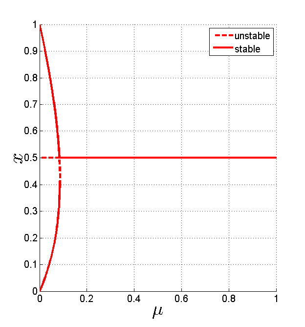
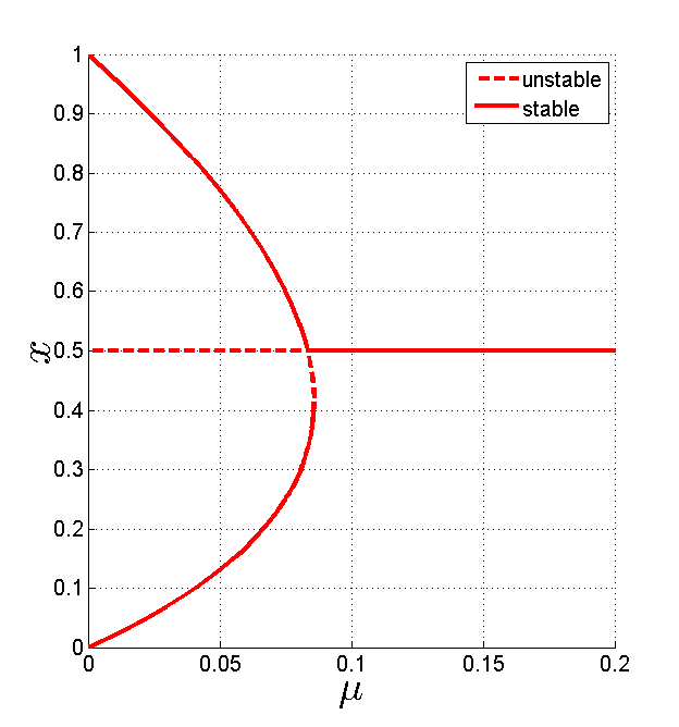
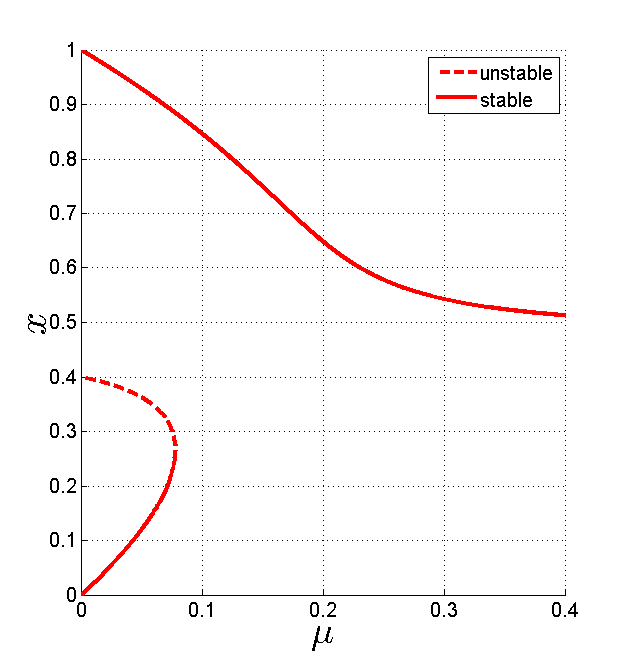
The stability of these equilibria depend on the value of $\mu$. When $\mu=0$ the equilibria are $x_{-}(0)=0$, $x_{0}(0)=1/2$, and $x_{+}(0)=1$ with $x_{-}(0)$ and $x_{+}(0)$ being stable and $x_{0}(0)$ unstable. The equilibria maintain these stabilities until the first bifurcation point, $\mu_{1}$. This bifurcation point occurs when either $x_{-}(\mu)$ or $x_{+}(\mu)$ intersects $x_{0}(\mu)$. Assuming $a>d$ and $b<c$, this intersection occurs between $x_{+}(\mu)$ and $x_{0}(\mu)$ resulting in $x_{+}(\mu)$ becoming unstable and $x_{0}(\mu)$ becoming stable. Solving for this intersection, we find $\mu_{1}=\frac{d-b}{2(a+d)}$. The second bifurcation value, $\mu_{2}$, occurs when $x_{-}(\mu)$ and $x_{+}(\mu)$ become complex-valued leaving $x_{0}(\mu)$ as the only stable equilibrium. We find $\mu_{2}=(d-b)(a+d-2\sqrt{ad})/(d-a)^{2}$. (Note that in case 1.3, there is complete symmetry and $\mu_{1}=\mu_{2}$). This analysis completely determines the bifurcation diagrams for case 1.1. The bifurcation diagram will have the same qualitative behavior as Figure 3.

Figure 3: Bifurcation diagram for case 1.1, $a=4,b=1,c=3,d=2$. Left frame is $\mu\in(0,1)$ and the right frame is a blowup. Compare this figure to Figure 1.

3.2 Case 2 — $a+b>c+d$

It is no longer possible to factor $f(x;\mu)$, but we can use the Implicit Function Theorem to describe the motion of the equilibria. When $\mu=0$, equilibria occur at

$$x_{-}(0)=0,\quad x_{0}(0)=\frac{d-b}{a-b-c+d},\quad x_{+}(0)=1,$$

again with with $x_{-}(0)$ and $x_{+}(0)$ being stable and $x_{0}(0)$ unstable. If $x(\mu)$ is an equilibrium of the deterministic equation then the Implicit Function Theorem implies

$$\frac{dx(\mu)}{d\mu}=-\frac{\dfrac{\partial f}{\partial\mu}(x;\mu)}{\dfrac{\partial f}{\partial x}(x;\mu)}$$

The only real root of $\dfrac{\partial f}{\partial\mu}(x;\mu)$ between $0$ and $1$ is

$$x_{*}=\frac{-(b-c+2d)+\sqrt{(b-c)^{2}+4ad}}{2(a-b+c-d)}.$$

By observing that

$$\frac{\partial f}{\partial\mu}(x_{-}(0);0)=1>0,\quad\frac{\partial f}{\partial\mu}(x_{+}(0);0)=-1<0$$

we find that $\dfrac{\partial f}{\partial\mu}(x)>0$ for $x<x_{*}$ and $\dfrac{\partial f}{\partial\mu}(x)<0$ for $x>x_{*}$. The roots of $\dfrac{\partial f}{\partial x}(x,\mu)$ occur when

$$\mu_{*}(x)=\frac{p(x)}{q(x)},$$

where

By observing that

$$\frac{\partial f}{\partial x}(0,0) =\frac{b}{d}-1<0$$

$$\frac{\partial f}{\partial x}(x_{0}(0),0) =-\frac{(a-c)(b-d)}{ad-bc}>0$$

$$\frac{\partial f}{\partial x}(1,0) =\frac{c}{a}-1<0$$

and that $\mu_{*}(x)$ is concave down we find that $\mu_{*}$ is a parabola in the $\mu$-$x$ plane. Therefore $\frac{\partial f}{\partial x}(x,u)>0$ for $\mu<\mu_{*}(x)$ and $\frac{\partial f}{\partial x}(x,u)<0$ for $\mu>\mu_{*}(x)$.

Figure 4: Sign of $dx/du$ for $a+b>c+d$

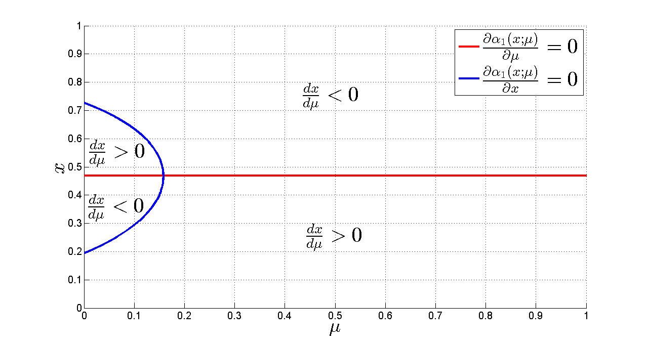
Putting the information about $\frac{\partial f}{\partial\mu}(x)$ and $\frac{\partial f}{\partial x}(x,\mu)$ together, there are $4$ regions where $\frac{dx}{d\mu}$ changes sign. The first equilibrium $x_{-}(\mu)$ starts at $0$ which is located in a region where $\frac{dx}{d\mu}>0$ and is therefore increasing. It is easy to show that $x_{0}(0)<x_{*}$ and thus $x_{0}(\mu)$ starts in a region where $\frac{dx}{d\mu}<0$. Therefore $x_{0}(\mu)$ is always decreasing. Similarly $x_{+}(\mu)$ starts in a region where $\frac{dx}{d\mu}<0$ and therefore is always decreasing. A bifurcation point occurs at the value of $\mu$ when two of the equilibria become complex valued. By continuity, this must occur along $u_{*}(x)$ when $x_{+}(\mu)$ and $x_{0}(\mu)$ collide. The bifurcation diagram described by the motion of these equilibria has the qualitative behavior as Figure 5.

Figure 5: Bifurcation Diagram of case 2: $a=4,b=2,c=1,d=4$

4 Stochastic Analysis

Section 3 described the deterministic behavior of the process in the $N\to\infty$ limit. However, if $N\gg 1$ but finite, the Markov chain model with retain stochasticity, although of course the variance of this process will vanish as $N\to\infty$.

In this section, we study this random process for $N$ large but finite, using the standard tools [Gar04]. The two main asymptotic expansions used here are the “diffusion approximation” and the “WKB expansion”, which roughly go as follows. In both cases, we assume that we start off with a Master equation for the stochastic process after a system size scaling, specifically we write

$$\frac{\partial P(i,t)}{\partial t}=\omega_{+}(i-1)P(i-1,t)+\omega_{-}(i+1)P(i+1,t)-(\omega_{+}(i)+\omega_{-}(i))P(n,t)$$ (4.1)

with reflecting boundary conditions at $i=0$ and $i=N$. In terms of the scaled variable $x=i/N$, this master equation is

$$\begin{split}\frac{\partial P(x,t)}{\partial t}&=N\Omega_{+}(x-1/N)P(x-1/N,t)+N\Omega_{-}(x+1/N)P(x+1/N,t)\\ &\quad-N(\Omega_{+}(x)+\Omega_{-}(x))P(x,t).\end{split}$$ (4.2)

In the diffusion approximation, one simply makes a Taylor series expansion of (4.2) and then truncates at second order, which gives a Fokker–Planck PDE. One can then consider the paths of this Fokker–Planck equation which are governed by an SDE. Computing the stationary distribution and the jumping timescale then corresponds to solving this PDE with particular boundary conditions. In particular, since the system is one-dimensional, it can be written in the form of a diffusion in a one-dimensional potential $\Phi$. This potential governs the dynamics of this system, and in particular governs the switching times of the system from one basin to another.

In the WKB approximation, the procedure is more complex. We seek to understand how the distribution of an initial condition placed near one attractor will behave. The motivating presumption is that it will settle down to a characteristic shape inside the basin of attraction of this point, and this shape will decay to zero on a timescale associated with the escape of trajectories out of this basin. More concretely: We first assume that the solution of the Master equation assuming that the initial condition is at $x_{-}$ w.p.1 can be written in quasistationary form,

$$\Pi(x,t)=e^{-t/\tau_{-}}\exp\left(N\Psi_{-1}(x)+\Psi_{0}(x)+N^{-1}\Psi_{1}(x)+\cdots\right),$$

where $\tau_{-}$ is the yet-to-be-determined jumping timescale. If we truncate the above expression to remove terms of order $N^{-1}$, we obtain the quasistationary distribution

$$\widehat{\Pi}(x):=e^{t/\tau_{-}}\Pi(x,t)=k(x)e^{-N\Psi_{-1}(x)},\quad\log k(x)=\Psi_{0}(x).$$

We drop the subscript on $\Psi_{-1}$ in the sequel. Here the function $\Psi$ plays the role of a potential, similar to $\Phi$ in the diffusion approximation and is also called the quasipotential for the system. The distribution $\widehat{\Pi}(x)$ is not a stationary distribution, since it will decay on the long timescale $\tau_{-}^{-1}$, but the idea is that the solution relaxes very quickly to $\widehat{\Pi}(x)$, and then decays slowly to zero. One can perform an asymptotic expansion in inverse powers of $N$ to obtain equations for $k,\Psi,\tau_{-}$, see details below.

It is known [Bre14, Bre10] that the WKB expansion gives an asymptotically correct expression for the jumping timescale, whereas the diffusion approximation gives a slightly different, and wrong expression, but we observe two things for this problem: first, the diffusion approximation is much simpler to compute, and second, the answers obtained from the numerics show that the two answers are indistinguishable on the types of problems that we can simulate.

4.1 Diffusion Approximation

Performing a Taylor expansion on (4.2) in powers of $1/N$ results in

$$\frac{\partial P(x,t)}{\partial t}=\sum_{n=1}^{\infty}N^{1-n}\frac{(-1)^{n}}{n!}\frac{\partial^{n}}{\partial x^{n}}\left[\alpha_{n}(x)P(x)\right]$$ (4.3)

where $\alpha_{n}(x)=\Omega_{+}(x)+(-1)^{n}\Omega_{-}(x)$. Terminating this series to order $1/N$ and writing $f=\alpha_{1},\sigma=\alpha_{2}$ results in the diffusion approximation

$$\frac{\partial P(x,t)}{\partial t}=-\frac{\partial}{\partial x}\left[f(x)P(x)\right]+\frac{1}{2N}\frac{\partial^{2}}{\partial x^{2}}\left[\sigma(x)P(x)\right]=:\mathcal{L}^{*}P$$ (4.4)

The diffusion approximation is a Fokker-Planck equation and has the equivalent SDE form

$$dx=f(x)\ dt+\sqrt{\frac{\sigma(x)}{N}}\ dW(t).$$ (4.5)

As $N\rightarrow\infty$, this is exactly the deterministic equation (3.1) discussed in section 3.

4.1.1 Linear noise Approximation

The linear noise approximation, more commonly known as the van Kampen expansion [VK92, VK82, Gar04]. The idea here is to write $x(t)=\varphi(t)+N^{-1/2}z$, obtain equations for $z$ , then assume that $\varphi(t)$ has some well-defined limit as $t\to\infty$. In the case where the deterministic system has a unique attracting fixed point $x^{*}$, applying the van Kampen expansion (see Appendix A.1 for more detail, we obtain

$$\mathbb{E}[x(t)]\to x^{*},\quad{\rm{Var}}(x(t))\to\frac{\sigma(x_{*})}{2N\left|{f^{\prime}(x_{*})}\right|}.$$ (4.6)

This computation is simple and gives useful information: in particular we obtain the scaling of the variance as a function of $N$. The one issue with this approximation is that it is guaranteed to be Gaussian and thus cannot capture the skew of the original process.

4.1.2 Higher-order Moments

The linear noise approximation is the lowest order expansion for the diffusion approximation, but this can be extended to a general perturbation expansion on (4.5). Writing

$$x(t)=x_{*}+N^{-1}x_{1}(t)+N^{-2}x_{2}(t)+\dots$$

and truncating at second order, we obtain for large $t$ (see Section A.2 for details):

$$\mathbb{E}[x(t)]\to x_{*}+\frac{f^{\prime\prime}(x_{*})\sigma(x_{*})}{4N(f^{\prime}(x_{*}))^{2}},$$ (4.7)

$${\rm{Var}}(x(t))\to\frac{\sigma(x_{*})}{2N\left|{f^{\prime}(x_{*})}\right|}+\frac{(f^{\prime\prime}(x_{*}))^{2}\sigma^{2}(x_{*})}{8N^{2}(f^{\prime}(x_{*}))^{4}}+\frac{(\sigma^{\prime}(x_{*}))^{2}}{16N^{2}(f^{\prime}(x_{*}))^{2}},$$ (4.8)

$$\mathbb{E}[(x(t)-\mathbb{E}[x(t)])^{3}]\to\frac{(f^{\prime\prime}(x_{*}))^{3}\sigma(x_{*})^{3}}{8N^{3}f^{\prime}(x_{*})^{6}}+\frac{3(\sigma^{\prime}(x_{*}))^{2}f^{\prime\prime}(x_{*})\sigma(x_{*})}{32N^{3}f^{\prime}(x_{*})^{4}}.$$ (4.9)

This next approximation gives additional insight into our process for case 1. In section 3, we determined that once $\mu\geq\mu_{2}$, there is one stable equilibria at $x_{0}=1/2$. At this equilibrium, both strategies have the same proportions, but the sign of the centered third moment can give insight into which strategy has a slight advantage. For now, we will just determine the sign of the centered third moment. Around the equilibria $x_{0}=1/2$, equation (4.9) simplifies to

$$\mathbb{E}[(x-\mathbb{E}[x])^{3}]=\frac{(f^{\prime\prime}(x_{0}))^{3}}{64N^{3}f^{\prime}(x_{0})^{6}}$$

The sign of this only depends on the sign of $f^{\prime\prime}(x_{0})$. Using the fact that $a+b=c+d$ we can factor $f^{\prime\prime}(x_{0})$ as

$$f^{\prime\prime}(x_{0})=\frac{32(c+d)(a-c)(a-d)(2\mu-1)}{(a+b+c+d)^{3}}$$

The sign of the skew is now easily found.

$$\begin{array}[]{c|cc}&\mu_{2}<\mu<.5&\mu>.5\\ \hline\cr a>d&\mathbb{E}[(x-\mathbb{E}[x])^{3}]<0&\mathbb{E}[(x-\mathbb{E}[x])^{3}]>0\\ a<d&\mathbb{E}[(x-\mathbb{E}[x])^{3}]>0&\mathbb{E}[(x-\mathbb{E}[x])^{3}]<0\end{array}$$

4.1.3 Stationary Distribution

Setting the left-hand side of equation (4.4) to 0 and using the reflecting boundary conditions, it is straightforward to find the stationary distribution for the diffusion approximation:

$$P_{s}(x)=\frac{\mathcal{B}e^{-N\Phi(x)}}{\sigma(x)}$$ (4.10)

where $\mathcal{B}$ is a normalization constant and the quasipotential if the function $\Phi(x)=-2\int_{0}^{x}\frac{f(x^{\prime})}{\sigma(x^{\prime})}\ dx^{\prime}$. By differentiating equation (4.10) and neglecting the $1/N$ terms, one sees that for large $N$, the maxima of the stationary distribution occur at the stable fixed points of the deterministic equation (3.1), while the minima of the stationary distribution occur at the unstable fixed points of the deterministic equation (3.1).

4.1.4 First-Passage Times using Diffusion

Here we see to compute the mean first passage time (MFPT) from $x_{-}$ to $x_{+}$ using (4.4).

To calculate the MFPT from $x_{-}$ to $x_{+}$ we restrict our attention to the interval $[0,x_{+}]$ and impose a reflecting boundary conditions at $0$ and absorbing boundary conditions at $x_{+}$. Let $T(x)$ denote the first passage time (FPT) at which the system reached $x_{+}$ starting at $x$ and $\tau_{-}(x)=\mathbb{E}[T(x)]$ denote the MFPT from $x$ to $x_{+}$. The MFPT satisfies

$$\mathcal{L}\tau_{-}+1=0,\quad\tau_{-}^{\prime}(0)=0,\quad\tau_{-}(x_{+})=0,$$ (4.11)

where

$$\mathcal{L}:=f(x)\frac{\partial}{\partial x}+\frac{\sigma(x)}{2N}\frac{\partial^{2}}{\partial x^{2}}$$

is the (formal) adjoint of the Fokker–Planck operator defined in (4.4). This follows from the fact that $\mathcal{L}$ is the generator of the diffusion process [Gar04]. Since the coefficients of the diffusion are known explicitly, we can obtain a formula for $\tau_{-}(x)$ by quadrature and apply Laplace’s integral method (see Appendix A.3 for details) to obtain

$$\tau_{-}=\frac{2\pi}{\Omega_{+}(x_{-})\sqrt{\Phi^{\prime\prime}(x_{-})|\Phi^{\prime\prime}(x_{0})|}}e^{N(\Phi(x_{0})-\Phi(x_{-}))}.$$ (4.12)

Notice in particular that this approximation is independent of $x$ as long as it is not too close to $x_{0}$. Thus we can think of the quantity $\tau_{-}$ as the MFPT for any initial condition starting in a neighborhood of $x_{-}$ to reach a neighborhood of $x_{+}$.

We can perform the same computation in the other direction to obtain

$$\tau_{+}=\frac{2\pi}{\Omega_{-}(x_{+})\sqrt{\Phi^{\prime\prime}(x_{+})|\Phi^{\prime\prime}(x_{0})|}}e^{N(\Phi(x_{0})-\Phi(x_{+}))}.$$ (4.13)

4.2 WKB Approximation

We seek a quasistationary distribution of the master equation (4.2) in the form

$$\Pi(x,t)=k(x)e^{-N\Psi(x)}e^{-t/\tau_{-}}.$$ (4.14)

If we plug this Ansatz into the Master equation (4.2), Taylor expand $k,\Psi$ in powers of $N^{-1}$ (see appendix A.4 for details), and assume that $\tau_{-}\gg N$, then we obtain two solutions for the WKB solution, called the relaxation and activation solutions:

$$\Pi_{\mathsf{rel}}(x) =\frac{B}{\Omega_{+}(x)-\Omega_{-}(x)},$$ (4.15)

$$\Pi_{\mathsf{act}}(x) =\frac{A}{\sqrt{\Omega_{+}(x)\Omega_{-}(x)}}e^{-N\Psi(x)},\quad\Psi(x)=\int_{0}^{x}\ln\left(\frac{\Omega_{-}(x^{\prime})}{\Omega_{+}(x^{\prime})}\right)\ dx^{\prime}..$$ (4.16)

These solutions have a total of two free constants to be determined. Performing a matched asymptotic expansion around the point $x_{0}$ (again see appendix A.4 for details), we obtain the formula

$$\tau_{-}=\frac{2\pi}{\Omega_{+}(x_{-})\sqrt{|\Psi^{\prime\prime}(x_{0})|\Psi^{\prime\prime}(x_{-})}}e^{N(\Psi(x_{0})-\Psi(x_{-}))}$$ (4.17)

Similarly, the MFPT from $x_{+}$ to $x_{-}$ is

$$\tau_{+}=\frac{2\pi}{\Omega_{-}(x_{+})\sqrt{|\Psi^{\prime\prime}(x_{0})|\Psi^{\prime\prime}(x_{+})}}e^{N(\Psi(x_{0})-\Psi(x_{+}))}$$ (4.18)

4.3 Comparison of quasipotentials

It is useful to compare the expressions (4.12) and (4.17); notice that the only difference is that there is a different quasipotential: $\Phi$ for the diffusion approximation and $\Psi$ for the WKB approximation. We repeat these here for comparison:

$$\Phi(x)=\int_{0}^{x}-2\frac{\Omega_{+}(x^{\prime})-\Omega_{-}(x^{\prime})}{\Omega_{+}(x^{\prime})+\Omega_{-}(x^{\prime})}\,dx^{\prime},\quad\Psi(x)=\int_{0}^{x}\log\left(\frac{\Omega_{-}(x^{\prime})}{\Omega_{+}(x^{\prime})}\right)\,dx^{\prime}.$$

Now first notice that the only way in which $\Phi,\Psi$ appear in the timescale is through the difference of values at $x_{0}$ and $x_{-}$, so in fact we are really concerned with the numbers we obtain when we evaluate these integrals from $x_{-}$ to $x_{0}$.

These integrands are certainly different functions and there is no reason why they should be close. However, let us write $q(x)=\Omega_{-}(x)/\Omega_{+}(x)$, and expand each integrand in a Taylor series at $q=1$:

$$\Phi^{\prime}(x)=-2\frac{1-q}{1+q}=\sum_{k=1}^{\infty}\frac{(-1)^{k-1}}{2^{k-1}}(q-1)^{k},\quad\Psi^{\prime}(x)=\log(q)=\sum_{k=1}^{\infty}\frac{(-1)^{k-1}}{k}(q-1)^{k}$$

Note that these expressions are equal up to the third order term in $(q-1)$, and thus as long as $\Omega_{+}(x)$ and $\Omega_{-}(x)$ are close, then we expect these two integrals to be close.

Figure 6: Comparison of the quasipotentials $\Phi(x),\Psi(x)$ for particular parameter values $a=4,b=1,c=3,d=2,\mu=0.05$. The left frame shows the two functions on the same axis, and the right frame shows their difference.

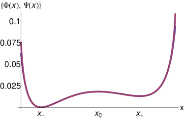
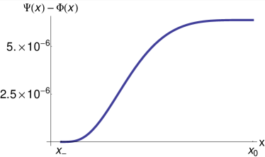
In particular, we plot the two quasipotentials for the parameters $a=4,b=1,c=3,d=2,\mu=0.05$ in Figure 6. Note that the two functions are indistinguishable except for near the ends of the domain. Considering the difference on the interval $[x_{-},x_{0}]$, and we see that the difference between the functions is four orders of magnitude smaller than the functions themselves.

Now, of course, when $N\to\infty$, the quasipotentials are multiplied by $N$ and exponentiated, so that even a small difference in the quasipotential will make a huge difference asymptotically. However, we should note that both approximations are only expected to be accurate in the limit $N\to\infty$, and for any finite but large $N$, the neglected terms in the expansion could dominate any difference in the quasipotentials. We actually see that this is so in the simulations presented below.

4.4 Simulation Results

4.4.1 Comparison between van Kampen approximation and deterministic system

This section compares the mean and variance of the simulations of the Markov process to the mean and variance calculated from the linear-noise approximation in section 4.1.1.

Recall that the mean of the linear noise approximation is given by the deterministic equation (3.1). Figure 7 compares the mean of the simulation of the Markov process against the bifurcation diagrams determined in section 3. We see that the deterministic equation is a good approximation of the mean of the process. The only location of disagreement is for $\mu$ close to the bifurcation values. Of course, as $N$ increases this will become more accurate.

Figure 7: Mean of Markov process versus predicted mean. In the left frame we have an example of Case 1.1, $a=4,b=1,c=3,d=2,N=2000$; in the right we have $a=4,b=1,c=2,d=4,N=2000$.

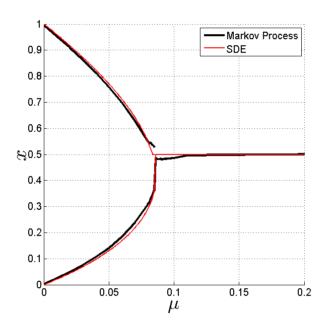
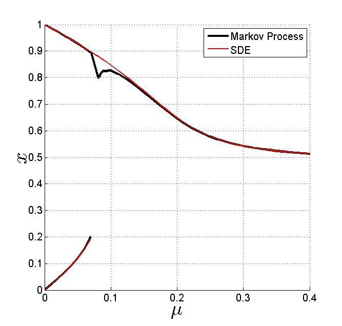
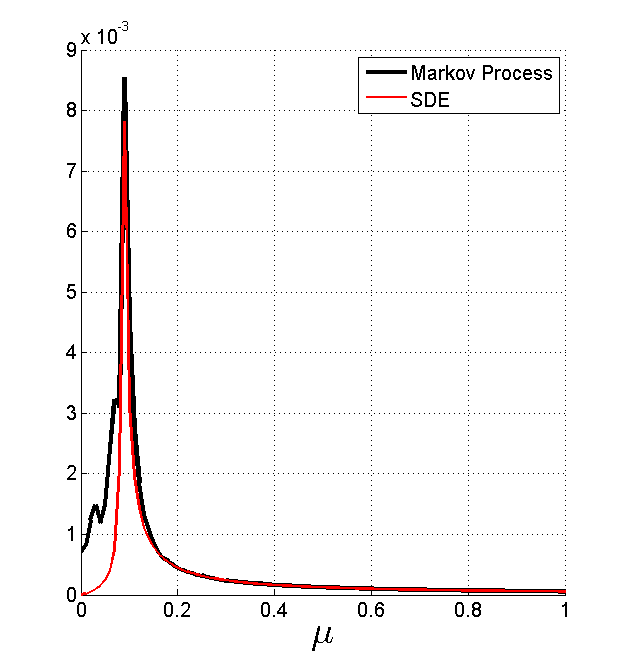
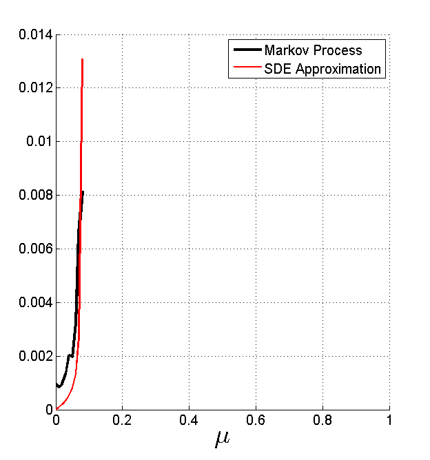
Figure 8 compares the conditional variance of the Markov process around each equilibrium point against equation (A.5). For the purposes of the figures, when there is only one equilibrium, we plot it on the $x_{-}$ figure. Similar to the mean, the figures differ slightly once $u$ gets close to the bifurcation points. Again this is due the size of $N$.

(a) Conditional variance around $x_{-}$

(b) Conditional variance around $x_{+}$

Figure 8: Conditional variance of case 1.1: $a=4,b=1,c=3,d=2,N=2000$.

4.4.2 Comparison of MFPT

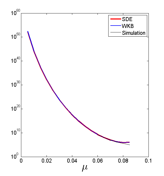
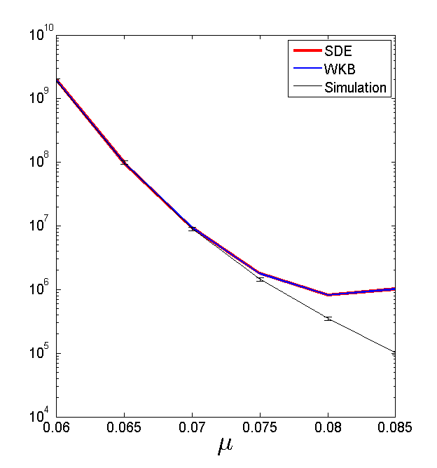
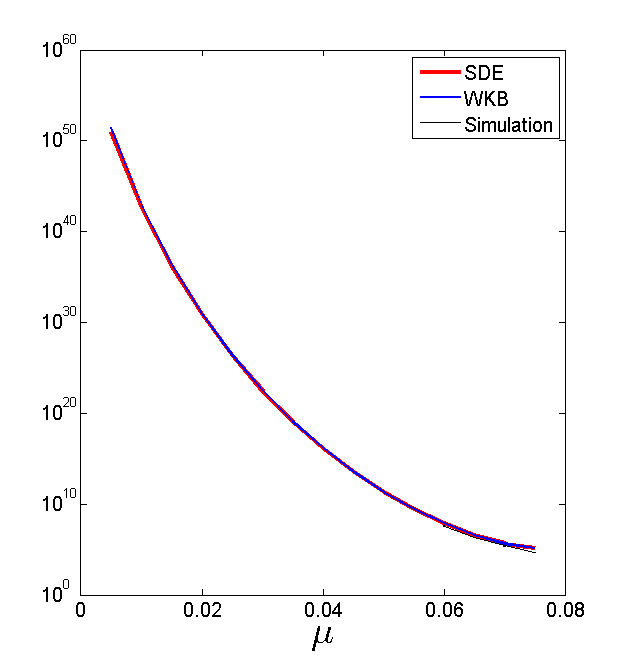
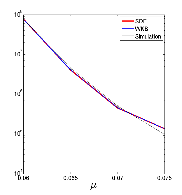
The MFPTs calculated from both the SDE approximation and WKB approximation differ in the prefactor and the form of the quasipotential. The MFPT calculated from the WKB approximation will more accurately capture the exponential time scale in which switching occurs in the limit as $N\to\infty$. However, in simulating both formulations we see they are indistinguishable. Simulations can only be done for relatively small $N$ due to the exponential stiffness of the problem, and we see that for any accessible simulation, the relative error is indistinguishable.

To give us an idea of the accuracy of these approximations, we use a Monte Carlo simulation of the Markov process: We averaged 1000 realizations of the Markov process to calculate the MFPT from $x_{-}$ to $x_{+}$. We know from both the SDE approximation (4.12) and the WKB approximation (4.17) that these MFPTs are exponentially large, which makes them hard to simulate using the Markov process.

We plot all of these in Figure 9. As $\mu\to 0$, the transition time becomes exponentially large, so the range of $\mu$ for which we can capture this transition time is quite restricted. In each row, we plot only those $\mu$ where we could perform a Monte Carlo simulation on the Markov chain directly in the right column. In the left column, we extend the plotting region down to small $\mu$.

For case 1.1, we were able to simulate the MFPT starting at $\mu=.06$. Figure compares the MFPT from $x_{-}$ to $x_{+}$ of the simulation of the Markov process (along with the $95\%$ confidence interval) to the MFPT approximated by the SDE and WKB approximations. Initially $\tau_{-}^{SDE}$ and $\tau_{-}^{WKB}$ are indistinguishable and both fall within the confidence interval of our simulated $\tau_{-}$. As $\mu$ approaches the bifurcation point, $\tau_{-}^{SDE}$ and $\tau_{-}^{WKB}$ are still indistinguishable, but they no longer fall within the confidence interval of $\tau_{-}$. This is due to the fact that $\tau_{-}^{SDE}$ and $\tau_{-}^{WKB}$ are good approximations when $N$ is large because the stationary distribution is sharply peaked around $x_{-}$ and $x_{+}$. The simulations we ran use $N=1000$ and as $\mu$ approaches the bifurcation point, the stationary distribution is not as sharply peaked, and we expect to need larger $N$ to make the asymptotics accurate.

Figure 9: MFPT from $x_{-}$ to $x_{+}$ in two cases: the top row is an example of case 1.1: $a=4,b=1,c=3,d=2,N=1000$, whereas the bottom row is an example of case 2: $a=4,b=2,c=1,d=4,N=1000$. In all cases we are plotting $\tau_{-}$, the transition time from $x_{-}$ to $x_{+}$. The right column is a blowup of the left.

5 Discussion

In this paper, we have studied a stochastic version of a standard game-theoretic model, concentrating on the case where there are multiple ESS strategies and when the population is small enough that stochastic effects need to be taken into account. Our dynamics also include a mutation parameter for offspring, and we prove that a large enough mutation factor always causes the multiple ESS solutions to merge. The presence of noise due to a finite population turns each ESS solution into a metastable solution, and we computed the asymptotics of the switching timescales between these.

We were able to completely characterize the bifurcation diagrams for this model when the system is in the infinite population limit. We also were able to make two nonintuitive observations about the stochastic process:

1. We see that the computation for the switching time using the diffusion approximation or the asymptotics directly on the Master equation give essentially the same results: specifically, we see in Figure 9 that the two approximations are indistinguishable over a wide range of parameters. What is perhaps more surprising is that these two agree even when they are far away from the actual answer gotten from Monte Carlo simulations — these approximations are more like each other than the quantity that they are seeking to approximate. Of course, the fact that these approximations deviate from the true value determined by Monte Carlo is not a contradiction, since these asymptotics are only guaranteed to be correct in the $N\to\infty$ limit. We also see from the same figure that this limit is very non-uniform in system parameters, e.g. for fixed $N$ the approximation has a different level of effectiveness for different $\mu$.

2. We also see that the stochastic system gives a finer picture of the dynamics than the deterministic limit does. For example, consider cases where $\mu$ is small enough that the system has multiple ESS states. In the deterministic regime ($N=\infty$), we have multiple stable solutions that will persist for all time, and in particular, the long-term steady state behavior will depend strongly on the initial condition of the system. For large $N$, however, the system will spend most of its time near these two solutions, but will switch between the two on the timescales computed in Section 4. Of course, in general the switching timescales in each direction will be different (often, significantly different) so this allows us to understand which of the two solutions are “more” stable, and which solution we will expect to observe more often. We also saw in Section 4.1.2 that the stochastic dynamics have a bias even when the deterministic dynamics are symmetric, so that the finite-size effects can lead to a bias; for example, the stochastic dynamics have a skew related to the self-interaction strength of each population.

6 Acknowledgments

L. D. was supported by the National Aeronautics and Space Administration (NASA) through the NASA Astrobiology Institute under Cooperative Agreement Number NNA13AA91A issued through the Science Mission Directorate. M. G. acknowledges support from National Science Foundation grant DMS 08-38434 “EMSW21-MCTP: Research Experience for Graduate Students.”

Appendix A Details of derivations above

A.1 van Kampen approximation

The linear noise approximation developed by van Kampen [VK92, VK82, Gar04] assumes the system has linear noise and further expands the diffusion approximation to obtain the lowest order expansion. The linear-noise expansion allows us to easily calculate the moments of this approximation. We begin by assuming

$$x=\phi(t)+N^{-1/2}z$$ (A.1)

where $z$ is a fluctuation term and $\phi(t)$ is not yet determined. Making this change of variables in equation (4.3), requiring $\phi(t)$ to satisfy $\phi^{\prime}(t)=f(\phi(t))$ (deterministic equation) and collecting only the $O(1)$ terms gives

$$\frac{\partial P(z,t)}{\partial\tau}=-f^{\prime}(\phi(t))\frac{\partial}{\partial z}\left[zP(z,t)\right]+\frac{1}{2}\sigma(\phi(t))\frac{\partial^{2}}{\partial z^{2}}\left[P(z,t)\right]$$ (A.2)

By multiplying equation (A.2) by $z$, integrating, and then integrating by parts the appropriate number of times, we find that $z$ is Gaussian with moment equations,

$$\frac{\partial}{\partial t}\mathbb{E}[z]=f^{\prime}(\phi(t))\mathbb{E}[z]$$ (A.3)

and

$$\frac{\partial}{\partial t}\mathbb{E}[z^{2}]=2f^{\prime}(\phi(t))\mathbb{E}[z^{2}]+\sigma(\phi(t)).$$ (A.4)

Assuming that if the process runs long enough, the first and second moments will eventually be stationary, and noting that $\phi(t)\to x^{*}$, we find

$$\mathbb{E}[z]=0,\quad\mathbb{E}[z^{2}]=-\frac{\sigma(x_{*})}{2f^{\prime}(x_{*})}.$$

where $x_{*}$ is an attracting fixed point of the deterministic equation. Making a change of variable back to $x$ results in,

$$\mathbb{E}[x]=\phi(t),\quad\mathbb{E}[x^{2}]=\phi^{2}(t)-\frac{\sigma(x_{*})}{2f^{\prime}(x_{*})}.$$

This shows that the mean of the linear noise approximation evolves according to the deterministic equation and the variance evolves according to

$${\rm{Var}}(x)=-\frac{\sigma(x_{*})}{2Nf^{\prime}(x_{*})}.$$ (A.5)

A.2 Higher-order corrections

We find higher order corrections to the moments of the linear noise approximation. We begin by assuming

$$x(t)=x_{*}(t)+\varepsilon x_{1}(t)+\varepsilon^{2}x_{2}(t)+\cdots$$

where $\varepsilon=\frac{1}{N}$. Plugging the Taylor expansion of $f(x)$ and $\sqrt{\sigma(x)}$ into the the SDE (4.5) and equating powers of $\varepsilon$, we obtain the following system of SDEs which can be solved iteratively.

$$dx_{0} =f(x_{*})\ dt,$$ (A.6)

$$dx_{1} =f^{\prime}(x_{*})x_{1}\ dt+\sqrt{\sigma(x_{*})}\ dW(t),$$ (A.7)

$$dx_{2} =\left(f^{\prime}(x_{*})x_{2}+\frac{f^{\prime\prime}(x_{*})x_{1}^{2}}{2}\right)\ dt+\frac{\sigma^{\prime}(x_{*})}{2\sqrt{\sigma(x_{*})}}x_{1}\ dW(t),\dots$$ (A.8)

Equation (A.6) is the deterministic equation and therefore $x_{*}$ is an equilibrium of the deterministic equation. Equations (A.7) and (A.8) are Ornstein–Uhlenbeck processes. Using the well known solution to an Ornstein–Uhlenbeck process and the Itô isometry we can calculate the centered moments of Equations (A.7) and (A.8) to obtain the first and second order corrections to moments calculated in the linear noise approximation:

$$\mathbb{E}[x]=x_{*}+\frac{f^{\prime\prime}(x_{*})\sigma(x_{*})}{4N(f^{\prime}(x_{*}))^{2}},$$ (A.10)

$${\rm{Var}}(x)=-\frac{\sigma(x_{*})}{2Nf^{\prime}(x_{*})}+\frac{(f^{\prime\prime}(x_{*}))^{2}\sigma^{2}(x_{*})}{8N^{2}(f^{\prime}(x_{*}))^{4}}+\frac{(\sigma^{\prime}(x_{*}))^{2}}{16N^{2}(f^{\prime}(x_{*}))^{2}},$$ (A.11)

$$\mathbb{E}[(x-\mathbb{E}[x])^{3}]=\frac{(f^{\prime\prime}(x_{*}))^{3}\sigma(x_{*})^{3}}{8N^{3}f^{\prime}(x_{*})^{6}}+\frac{3(\sigma^{\prime}(x_{*}))^{2}f^{\prime\prime}(x_{*})\sigma(x_{*})}{32N^{3}f^{\prime}(x_{*})^{4}}.$$ (A.12)

We can find any higher-order terms desired by continuing to solve the system of SDEs iteratively.

Note that to leading order, these are the moments obtained from the van Kampen approximation.

A.3 Laplace’s method

Equation (4.11) can be solved using integrating factors to find (q.v. (4.10)),

$$\tau(x)=2N\int_{x}^{x_{+}}e^{N\Phi(x^{\prime})}\int_{0}^{x^{\prime}}\frac{e^{-N\Phi(x^{\prime\prime})}}{B(x^{\prime\prime})}\ dx^{\prime\prime}\ dx^{\prime}.$$ (A.13)

For large $N$, $e^{-N\Phi(x)}$ is sharply peaked around $x_{-}$ and therefore $\int_{0}^{x^{\prime}}e^{-N\Phi(x^{\prime\prime})}\ dx^{\prime\prime}$ is nearly constant $x^{\prime}\in[x,x_{+}]$ for which $e^{N\Phi(x^{\prime})}$ is well above zero. With this assumption, equation (A.13) can be written as

$$\tau(x)=2N\int_{x}^{x_{+}}e^{N\Phi(x^{\prime})}\ dx^{\prime}\int_{0}^{x_{+}}\frac{e^{-N\Phi(x^{\prime\prime})}}{B(x^{\prime\prime})}\ dx^{\prime\prime}.$$ (A.14)

The first integral is sharply peaked around $x_{0}$ and the second integral is sharply peaked around $x_{-}$. Using a Gaussian approximation (that is, replacing $\Phi(\cdot)$ with its second-order Taylor expansion), and replacing the upper limits with any point strictly above $x_{0}$, we obtain the MFPT from $x_{-}$ to $x_{+}$ to be

A.4 WKB details

the following $O(1)$ and $O(\frac{1}{N})$ equations

$$0=\Omega_{+}(x)\left(e^{\Psi^{\prime}(x)}-1\right)+\Omega_{-}(x)\left(e^{-\Psi^{\prime}(x)}-1\right),$$ (A.15)

and

$$\begin{split}0&=\Omega_{+}(x)e^{\Psi^{\prime}(x)}\left(-\frac{k^{\prime}(x)}{k(x)}-\frac{\Psi^{\prime\prime}(x)}{2}\right)+\Omega_{-}(x)e^{-\Psi^{\prime}(x)}\left(\frac{k^{\prime}(x)}{k(x)}-\frac{\Psi^{\prime\prime}(x)}{2}\right)\\ &\quad-\Omega_{+}^{\prime}(x)e^{\Psi^{\prime}(x)}+\Omega_{-}^{\prime}(x)e^{-\Psi^{\prime}(x)}.\end{split}$$ (A.16)

The assumption that $\tau_{-}$ is large enough to not appear in these equations is not yet justified, but we show below that this is a self-consistent choice. Solving (A.15) for $\Psi(x)$ gives two solutions:

$$\Psi_{1}(x)=const,\quad\Psi_{2}(x)=\int_{0}^{x}\ln\left(\frac{\Omega_{-}(x^{\prime})}{\Omega_{+}(x^{\prime})}\right)\ dx^{\prime}.$$ (A.17)

Substituting each into the next order equation (A.16) and solving for $k(x)$ gives

$$k_{1}(x)=\frac{B}{\Omega_{+}(x)-\Omega_{-}(x)},\quad k_{2}(x)=\frac{A}{\sqrt{\Omega_{+}(x)\Omega_{-}(x)}}$$ (A.18)

We now seek to approximate $\tau_{-}$ in the quasistationary solution (4.14). Let us start with the Ansatz that the WKB approximation takes the form of the activation solution on $[0,x_{0}]$ as the process tries to escape the basin of attraction around $x_{-}$ and takes the form of the relaxation solution on $[x_{0},1]$ as the process is quickly attracted to $x_{+}$. The relaxation and activation solutions need to satisfy the matching boundary conditions at $x_{0}$, thus we match both to an appropriate inner solution at $x_{0}$ to find $A$ and $B$. Begin by rewriting the diffusion approximation as

$$\frac{\partial P(x,t)}{\partial t}=-\frac{\partial J(x,t)}{\partial x}$$ (A.19)

where

$$J(x,t)=(\Omega_{+}(x)-\Omega_{-}(x))P(x,t)-\frac{1}{2N}\frac{\partial}{\partial x}\left[(\Omega_{+}(x)+\Omega_{-}(x))P(x,t)\right].$$

Substituting the quasistationary solution $\Pi(x,t)=\widehat{\Pi}(x)e^{-t/\tau_{-}}$ into equation (A.19) and Taylor expanding around $x_{0}$ to order $1/N$ (again assuming that $\tau_{-}\gg N$) results in the constant flux through $x_{0}$,

$$J_{0}=(x-x_{0})(\Omega_{+}^{\prime}(x_{0})-\Omega_{-}^{\prime}(x_{0}))\widehat{\Pi}(x)-\frac{1}{N}(\Omega_{+}(x_{0}))\widehat{\Pi}^{\prime}(x)$$ (A.20)

where we have used the fact that $\Omega_{+}(x_{0})-\Omega_{-}(x_{0})=0$. It is straightforward to solve equation (A.20) with an integrating factor to find the inner solution,

$$\widehat{\Pi}_{inner}(x)=\frac{JN}{\Omega_{+}(x_{0})}e^{\frac{(x-x_{0})^{2}}{\sigma^{2}}}\int_{x}^{\infty}e^{-\frac{(y-x_{0})^{2}}{\sigma^{2}}}\ dy$$ (A.21)

where

$$\sigma=\sqrt{\frac{2\Omega_{+}(x_{0})}{N(\Omega_{+}^{\prime}(x_{0})-\Omega_{-}^{\prime}(x_{0}))}}$$

determines the size of the boundary layer. In order to match this inner solution with the activation and relaxation solutions, we use the following asymptotics of the inner solution:

$$\widehat{\Pi}_{inner}(x)=\begin{cases}\dfrac{NJ_{0}\sigma^{2}}{2(x-x_{0})\Omega_{+}(x_{0})}&x-x_{-}\gg\sigma\\ \dfrac{J_{0}N\sigma\sqrt{\pi}}{\Omega_{+}(x_{0})}e^{\frac{(x-x_{0})^{2}}{\sigma^{2}}}&x_{0}-x\gg\sigma\end{cases}$$ (A.22)

Expanding the relaxation solution (4.15) around $x_{0}$ and matching to the inner solution for $x-x_{0}\gg\sigma$ gives $J_{0}=B$. Expanding the activation solution around $x_{0}$ and matching to the inner solution for $x_{0}-x\gg\sigma$ gives

$$J_{0}=\frac{A\Omega_{+}(x_{0})}{\sqrt{\Omega_{+}(x_{0})\Omega_{-}(x_{0})}}\sqrt{\frac{|\Psi^{\prime\prime}(x_{0})|}{2\pi N}}e^{-N\Psi(x_{0})}$$

Substituting the quasistationary solution $\Pi(x,t)$ into the diffusion approximation and integrating over $[0,x_{0}]$, we link $\tau_{-}$ and $J_{0}$

$$\tau_{-}=\frac{1}{J_{0}}\int_{0}^{x_{0}}\widehat{\Pi}(x)\ dx$$ (A.23)

Using the activation solution on $[0,x_{0}]$ and a Gaussian approximation around $x_{-}$ results in

$$\tau_{-}=\frac{2\pi}{\Omega_{+}(x_{-})}\frac{1}{\sqrt{|\Psi^{\prime\prime}(x_{0})|\Psi^{\prime\prime}(x_{-})}}e^{N(\Psi(x_{0})-\Psi(x_{-}))}$$ (A.24)

References

- [AH81] Robert Axelrod and William Donald Hamilton, The evolution of cooperation, Science 211 (1981), no. 4489, 1390–1396.
- [ATG12] Hinrich Arnoldt, Marc Timme, and Stefan Grosskinsky, Frequency-dependent fitness induces multistability in coevolutionary dynamics, Journal of The Royal Society Interface 9 (2012), no. 77, 3387–3396.
- [Axe84] Robert Axelrod, The Evolution of Cooperation, Basic Books, 1984.
- [Axe97] Robert M. Axelrod, The complexity of cooperation: Agent-based models of competition and collaboration, Princeton University Press, 1997.
- [Bre10] Paul C. Bressloff, Metastable states and quasicycles in a stochastic Wilson-Cowan model of neuronal population dynamics, Physical Review E 82 (2010), no. 5, 051903.
- [Bre14] , Stochastic processes in cell biology, vol. 41, Springer, 2014.
- [Cro10] James F. Crow, Wright and Fisher on inbreeding and random drift, Genetics 184 (2010), no. 3, 609–611.
- [DN08] R.W.R. Darling and James R. Norris, Differential equation approximations for markov chains, Probability Surveys 5 (2008), 37–79.
- [Fel51] William Feller, Diffusion Processes in Genetics, Proc. Second Berkeley Symp. Math. Statist. Prob, vol. 227, 1951, p. 246.
- [Fis30] Ronald A. Fisher, The Genetical Theory of Natural Selection: a Complete Variorum Edition, Oxford University Press, 1930.
- [Gar04] C. W. Gardiner, Handbook of stochastic methods for physics, chemistry and the natural sciences, third ed., Springer Series in Synergetics, vol. 13, Springer-Verlag, Berlin, 2004. MR MR2053476 (2004m:00008)
- [GG08] Nicholas Guttenberg and Nigel Goldenfeld, Cascade of complexity in evolving predator-prey dynamics, Physical Review Letters 100 (2008), no. 5, 058102.
- [IFN07] Lorens A. Imhof, Drew Fudenberg, and Martin A. Nowak, Tit-for-tat or win-stay, lose-shift?, Journal of Theoretical Biology 247 (2007), no. 3, 574–580.
- [Kur72] Thomas G. Kurtz, Relationship between stochastic and deterministic models for chemical reactions, Journal of Chemical Physics 57 (1972), no. 7, 2976–2978.
- [Kur78] Thomas G. Kurtz, Strong approximation theorems for density dependent Markov chains, Stochastic Processes Appl. 6 (1977/78), no. 3, 223–240. MR MR0464414 (57 #4344)
- [ML75] Robert M. May and Warren J. Leonard, Nonlinear aspects of competition between three species, SIAM Journal on Applied Mathematics 29 (1975), no. 2, 243–253.
- [Mor58] Patrick A. P. Moran, Random Processes in Genetics, Mathematical Proceedings of the Cambridge Philosophical Society, vol. 54, Cambridge Univ Press, 1958, pp. 60–71.
- [NM92] Martin A. Nowak and Robert M. May, Evolutionary games and spatial chaos, Nature 359 (1992), no. 6398, 826–829.
- [Now06a] Martin A. Nowak, Evolutionary dynamics: Exploring the equations of life, Harvard University Press, 2006.
- [Now06b] , Five rules for the evolution of cooperation, Science 314 (2006), no. 5805, 1560–1563.
- [NS92] Martin A. Nowak and Karl Sigmund, Tit for tat in heterogeneous populations, Nature 355 (1992), no. 6357, 250–253.
- [NS05] , Evolution of indirect reciprocity, Nature 437 (2005), no. 7063, 1291–1298.
- [Smi82] John Maynard Smith, Evolution and the theory of games, Cambridge university press, 1982.
- [SW95] Adam Shwartz and Alan Weiss, Large deviations for performance analysis, Chapman & Hall, London, 1995.
- [TFSN04] Christine Taylor, Drew Fudenberg, Akira Sasaki, and Martin A Nowak, Evolutionary game dynamics in finite populations, Bulletin of Mathematical Biology 66 (2004), no. 6, 1621–1644.
- [VK82] N. G. Van Kampen, The diffusion approximation for markov processes, De Gruyter, 1982.
- [VK92] , Stochastic processes in physics and chemistry, vol. 1, Elsevier, 1992.
- [vNM53] John von Neumann and Oskar Morgenstern, Theory of games and economic behavior, Oxford UP, 1953.
- [Wei97] Jörgen W Weibull, Evolutionary game theory, MIT press, 1997.
- [WLCH08] Wen-Xu Wang, Jinhu Lü, Guanrong Chen, and PM Hui, Phase transition and hysteresis loop in structured games with global updating, Physical Review E 77 (2008), no. 4, 046109.
- [Wri31] Sewall Wright, Evolution in Mendelian Populations, Genetics 16 (1931), no. 2, 97.