Forecasts on neutrino mass constraints from the redshift-space two-point correlation function

Abstract

We provide constraints on the accuracy with which the neutrino mass fraction, $f_{\nu}$, can be estimated when exploiting measurements of redshift-space distortions, describing in particular how the error on neutrino mass depends on three fundamental parameters of a characteristic galaxy redshift survey: density, halo bias and volume. In doing this, we make use of a series of dark matter halo catalogues extracted from the BASICC simulation. The mock data are analysed via a Markov Chain Monte Carlo likelihood analysis. We find a fitting function that well describes the dependence of the error on bias, density and volume, showing a decrease in the error as the bias and volume increase, and a decrease with density down to an almost constant value for high density values. This fitting formula allows us to produce forecasts on the precision achievable with future surveys on measurements of the neutrino mass fraction. For example, a Euclid-like spectroscopic survey should be able to measure the neutrino mass fraction with an accuracy of $\delta f_{\nu}\approx 6.7\times 10^{-4}$, using redshift-space clustering once all the other cosmological parameters are kept fixed to the $\Lambda$CDM case.

1 Introduction

Estimating the neutrino mass is one of the main challenges of cosmology today. According to the standard model of particle physics, neutrinos are weakly interacting massless particles. However, the experiments on the oscillations of solar and atmospheric neutrinos tell us that neutrinos cannot be massless. Oscillation experiments can only measure the differences in the squared masses of the neutrino eigenstates $(m_{1},m_{2},m_{3})$ and not the absolute mass scale. The current data imply $|\Delta m_{31}^{2}|\simeq 2.4\times 10^{-3}\ \mathrm{eV}^{2}$ and $\Delta m_{21}^{2}\simeq 27.6\times 10^{-5}\ \mathrm{eV}^{2}$ (Beringer et al., 2012). These measurements provide a lower limit for the sum of neutrino masses of $\approx 0.06\ \mathrm{eV}$ (see Lesgourgues & Pastor 2014 for a review).

Now that cosmology has entered the “precision era” and the cosmological parameters can be constrained at a percent level, observations of the Universe can assist in the quest for neutrino mass, since neutrinos affect the evolution of the universe in several observable ways.

After thermal decoupling, relic neutrinos constitute a collisionless fluid, where the individual particles free-stream with the characteristic thermal velocity. As long as neutrinos are relativistic, the free-streaming scale is simply the Hubble radius. When they become non-relativistic, their thermal velocity decays, and the free-streaming scale is equal to (Lesgourgues & Pastor, 2014):

$$k_{FS}=0.82\frac{\sqrt{\Omega_{\Lambda 0}+\Omega_{m0}(1+z)^{3}}}{(1+z)^{2}}\frac{m_{\nu}}{1\mathrm{eV}}\ h\ \mathrm{Mpc}^{-1}\ ,$$ (1)

where $h\equiv H_{0}/(100\ \mathrm{km}\ \mathrm{s}^{-1}\mathrm{Mpc}^{-1})$ is the dimensionless Hubble parameter, $\Omega_{\Lambda 0}$ and $\Omega_{m0}$ are the cosmological constant and the matter density parameters, respectively, evaluated at $z=0$, and $m_{\nu}$ is the neutrino mass. The physical effect of free-streaming is to damp neutrino density fluctuations on scales $k\gg k_{FS}$, where neutrinos cannot cluster due to their large thermal velocity. This affects the matter power spectrum since neutrinos do not contribute, for $k>>k_{FS}$, to the gravitational potential wells produced by dark matter and baryons. Hence the power spectrum is reduced by a factor $\sim(1-f_{\nu})^{2}$, where

$$f_{\nu}\equiv\frac{\Omega_{\nu}}{\Omega_{m}}$$ (2)

is the neutrino mass fraction. For the same reason, the growth rate of dark matter perturbations is suppressed and acquires a scale dependence (Kiakotou et al., 2008).

The neutrino mass has non-trivial effects also on the cosmic microwave background (CMB) temperature anisotropies altering the redshift of matter-radiation equality, if $\Omega_{m}h^{2}$ is kept fixed. This translates into an overall modification of the amplitude and the location of the acoustic peaks. A change in the matter density would instead affect the angular diameter distance to the last scattering surface $D_{A}(z_{dec})$, and the slope of the CMB spectrum at low multipoles, due to the Integrated Sachs-Wolfe effect (Sachs & Wolfe 1967; Kofman & Starobinskij 1985). Many works attempted to measure neutrino mass combining different cosmological probes (e.g Wang et al. 2005; Seljak et al. 2006; Dunkley et al. 2009; Ichiki et al. 2009; Reid et al. 2010; Thomas et al. 2010; Komatsu et al. 2011; Saito et al. 2011; Sánchez et al. 2012; Hinshaw et al. 2009, 2013). One of the latest constraints come from recent Planck results (Planck Collaboration, 2015), that put an upper limit on the sum of neutrino masses, $\sum m_{\nu}<0.23\ \mathrm{eV}$. Using instead large scale structure probes, Beutler et al. (2014) find that $\sum m_{\nu}=0.36\pm 0.14\ \mathrm{eV}$, combining measurements from the Baryon Oscillation Spectroscopic Survey (BOSS) CMASS DR11 with WMAP9. So they exclude massless neutrinos at $2.6\sigma$, and including weak lensing and baryon acoustic oscillations (BAO) measurements the significance is increased to $3.3\sigma$.

Among large scale structure probes, redshift-space distortions (RSD) are one of the most promising ways to measure the neutrino mass. RSD are caused by galaxy peculiar velocities. When galaxy distances are computed from redshift measurements, assuming that the total velocity relative to the observer comes only from the Hubble flow, one obtains a distorted density field. This distortion effect is clearly imprinted in the two-point correlation function of galaxies. In particular, the iso-correlation contours appear squashed along the line of sight (LOS) on linear scales, while non-linear motions produce an elongation effect known as Fingers of God. The distortions on linear scales can be quantified by the distortion parameter

$$\beta(z)\equiv f(z)/b(z)\ ,$$ (3)

which is the ratio of the growth rate of structures and their linear bias factor. The parameter $\beta(z)$ is strictly related to the matter density parameter, since $f(z)=\Omega_{m}^{\gamma}(z)$, where $\gamma$ is the linear growth factor (Linder, 2005). Therefore, RSD provide the possibility to recover some important information about the dynamics of galaxies and the amount of matter in the Universe.

Massive neutrinos strongly affect the spatial clustering of cosmic structures: as shown, for instance, in Marulli et al. (2011), when assuming the same amplitude of primordial scalar perturbations, the average number density of large scale structures (LSS) is suppressed in the massive neutrino scenario, and the halo bias is enhanced with respect to the massless case. Moreover, the value of $f(z)$ decreases in the presence of massive neutrinos, due to their free-streaming which suppresses structure formation. Therefore, the value of $\beta$, which describes the cumulative effect of non-linear motions, is reduced by an amount that increases with $\sum m_{\nu}$ and $z$. Moreover, free-streaming massive neutrinos induce also a scale dependence in the parameter $\beta$. Finally, also the rms of the galaxy peculiar velocity is reduced with respect to the massless case, since both the growth rate $f(k,z)$ and the matter power spectrum enter the bulk flow predicted by linear theory (Elgarøy & Lahav 2005; Kiakotou et al. 2008).

At intermediate scales ($5\lesssim r[\mathrm{Mpc}/h]\lesssim 100$) and low redshifts, these effects are degenerate with the amplitude of the matter power spectrum, parameterised by $\sigma_{8}$. Indeed, the differences between the values of $\beta$ in a $\Lambda\mathrm{CDM}$ and a $\Lambda\mathrm{CDM}+\nu$ models are significantly reduced if the two cosmologies are normalised to the same value of $\sigma_{8}$. Nonetheless, the relative difference between the theoretical values of $\beta$ in these two models, at $z=1$, is $\delta\beta/\beta\simeq 3\%$, for $\sum{m_{\nu}}=0.6\ \mathrm{eV}$, which corresponds to the precision reachable by future redshift surveys in measuring the redshift space distortion parameter at $z<1$ (Marulli et al., 2011). RSD can thus contribute to constrain the total neutrino mass, helping to disentangle the degeneracies with other cosmological parameters.

The aim of this work is to exploit RSD to constrain cosmological parameters through a Markov Chain Monte Carlo (MCMC) procedure and make forecasts on the statistical accuracy achievable with future cosmological probes. Some attempts have been recently made to produce forecasts based on RSD using numerical simulations. For example, Guzzo et al. (2008) used mock surveys extracted from the Millennium simulation to estimate the errors affecting measurements of the growth rate. They found a scaling relation for the relative error on the $\beta$ parameter as a function of the survey volume and mean density. This formula has been later refined by Bianchi et al. (2012). The authors analysed the same catalogues of dark matter haloes used in the present work, extracted from a snapshot of the BASICC simulation (Angulo et al., 2008) at $z=1$, finding that the parameter $\beta$ can be underestimated by up to $10\%$, depending on the minimum mass of the considered haloes. They also proposed a new fitting formula, that aims at separating the dependence of the statistical error on bias, density and volume:

$$\frac{\delta\beta}{\beta}\approx Cb^{0.7}V^{-0.5}\exp\left(\frac{n_{0}}{b^{2}n}\right)\ ,$$ (4)

where $n_{0}=1.7\cdot 10^{-4}\,h^{3}\mathrm{Mpc}^{-3}$ and $C=4.9\cdot 10^{2}\,h^{-1.5}\mathrm{Mpc}^{1.5}$.

Here we follow a similar approach to study how the error on cosmological parameters depends on the survey parameters, focusing in particular on the neutrino mass fraction. The main differences with respect to the work of Bianchi et al. (2012) are the following:

• we use a theoretical real-space correlation function obtained from the dark matter power spectrum instead of the deprojected one;

• we use the multipoles of the correlation function rather than the full two-dimensional correlation function;

• we use an MCMC likelihood analysis to estimate parameters.

The combination of monopole and quadrupole is fundamental to break the degeneracy between the halo bias and $f_{\nu}$, and thus to constrain the neutrino mass fraction, as we will discuss later in detail.

This paper is organised as follows. In §2 we describe the BASICC simulation and the method adopted to select the subsamples. In §3 we describe the modellisation of the correlation function, the construction of the covariance matrix, and the approach used for the estimation of the best-fit parameters. In §4 we present our results, showing the dependence of the errors on the simulation parameters, providing a fitting formula similar to Eq. (4). Finally, in §5 we draw our conclusions.

2 Halo catalogues from the BASICC simulation

One of the building blocks of our work is the BASICC simulation, the Barionic Acoustic oscillation Simulation produced at the Institute for Computational Cosmology (Angulo et al., 2008). One of the advantages of using numerical simulations is that we know a priori the value of the parameters we want to measure. Moreover, simulations solve the problem of having only one Universe available for observations. Indeed it is possible to construct many mock catalogues, assuming the same cosmological parameters, and repeat the measurements for each of them. In particular, comparing the theoretical values of the parameters we want to measure with the mean of their measured estimates, we can assess the systematic errors due to the method, while the scatter between measurements gives us an estimate of the expected statistical errors.

The BASICC simulation has been explicitly designed to study BAO features in the clustering pattern, so its volume is large enough to follow the growth of fluctuations on a wide range of scales. At the same time, its mass resolution is high enough to allow splitting the whole box in sub-cubes with the typical volumes of ongoing surveys, still preserving a good statistics on the scales which are central in the present analysis. The BASICC simulation is made up by $1448^{3}$ dark matter particles of mass $M_{part}=5.49\times 10^{10}\,h^{-1}\,M_{\odot}$, in a periodic box of side $1340\,h^{-1}\text{Mpc}$. The cosmological model adopted is a $\Lambda CDM$ model with $\Omega_{m}=0.25$, $\Omega_{\Lambda}=0.75$, $\sigma_{8}=0.9$ and $h=H_{0}/(100\,\text{km}\,\text{s}^{-1}\,\text{Mpc}^{-1})=0.73$. The dark matter haloes are identified using a Friends-of-Friends (FOF) algorithm (Davis et al., 1985) with a linking length of $0.2$ times the mean particle separation. We consider only haloes with a minimum number of particles per halo of $N_{part}=20$, so that the minimum halo mass is $M_{halo}=20\cdot M_{part}\simeq 1.1\times 10^{12}\ h^{-1}\ M_{\odot}$.

Table 1: Properties of the halo catalogues used in the analysis. $N_{part}$ is the minimum number of particles per halo; $M_{cut}$ is the corresponding threshold mass; $\mathcal{N}_{tot}$ is the number of haloes with $M_{halo}\geq M_{cut}$; $n$ is the number density, computed as $\mathcal{N}_{tot}/V$, where $V=(1340\ h^{-1}\mathrm{Mpc})^{3}$ is the simulation volume; $b$ is the bias value.

$N_{part}$	$M_{cut}\times 10^{-12}$	$\mathcal{N}_{tot}$	$n\times 10^{5}$	$b$
	$[h^{-1}\ M_{\odot}]$		$[h^{3}\ \text{Mpc}^{-3}]$
$20$	$1.10$	7483318	$311$	$1.44$
$63$	$3.46$	2164960	$90.0$	$1.80$
$136$	$7.47$	866034	$36.0$	$2.15$
$236$	$13.0$	423511	$17.6$	$2.49$
$364$	$20.0$	230401	$9.58$	$2.89$

Table 2: Sub-samples used in our analysis to explore the dependence of the errors on mean density, bias and volume. Each sample is characterised by given values of the mean density, $n$, and the mass threshold, $M_{cut}$, (or the bias, $b$). The full, non-diluted, samples coincide with the bottom entry of each column. The entries in the table identified by circles represent the samples used to test the dependence of the errors on the survey volume. For these samples the simulation box has been split in $N^{3}$ sub-boxes with $N=\{4,5,6\}$, whereas for the other sub-samples (asterisks) we only consider $N=3$.

		$M_{cut}\times 10^{-12}\ [h^{-1}\ M_{\odot}]$
		$1.10$	$3.46$	$7.47$	$13.0$	$20.0$
	6.87	$\ast$	$\ast$	$\ast$	$\ast$	$\ast$
	9.58	$\ast$	$\ast$	$\ast$	$\ast$	$\ast$
	12.1	$\ast$	$\ast$	$\ast$	$\ast$
	17.6	$\ast$	$\ast$	$\ast$	$\ast$
	24.8	$\circ$	$\circ$	$\circ$
$n\times 10^{5}$	36.0	$\ast$	$\ast$	$\ast$
$[h^{3}\,\text{Mpc}^{-3}]$	58.7	$\ast$	$\ast$
	90.0	$\circ$	$\ast$
	131	$\ast$
	204	$\ast$
	311	$\circ$

In the present work, we consider the snapshot at $z=1$, that is the central value in the range of redshifts that will be explored in future redshift surveys, and select halo catalogues with different mass thresholds (i.e. different minimum number of particles per halo), which means different bias values. The properties of these catalogues are summarised in Table 1. This selection allows us to study the dependence of the error on the sample bias. Moreover, in order to investigate also the dependence of the errors on the halo density, the samples have been diluted to create a series of catalogues with decreasing density, down to a value of $\sim 7\times 10^{-5}h^{3}\ \text{Mpc}^{-3}$, at which the shot noise starts to dominate (see Bianchi et al. 2012). For each of these samples with varying bias and density, we split the simulation box in $3^{3}$ sub-boxes, obtaining $27$ sub-boxes. For some samples we also split the box in $N^{3}$ parts with $N=\{4,5,6\}$, in order to explore the error dependence on the volume, as shown in Table 2.

Figure 1: Monopole $\xi_{0}$ (left panel) and quadrupole $\xi_{2}$ (right panel) of the correlation function, multiplied by $r^{2}$. The grey dashed lines represent the multipoles measured from the $27$ mocks extracted from the catalogue with a mass threshold of $M_{cut}=1.1\times 10^{12}\ h^{-1}\ M_{\odot}$. The blue solid lines represent the multipoles averaged over the $27$ mocks, the error bars being the square root of the diagonal elements of the covariance matrix. The best-fit mean model is represented by the magenta dot-dashed lines.

3 Methodology

In this section we describe the method adopted to measure the correlation function from the mock catalogues, the modellisation of the correlation function and its multiploes, and the computation of the covariance matrix needed for the likelihood analyses.

3.1 Correlation function measurement

The two-dimensional two-point correlation function has been evaluated using the Landy & Szalay (1993) estimator:

$$\xi(r_{p},\pi)=\frac{HH(r_{p},\pi)-2HR(r_{p},\pi)+RR(r_{p},\pi)}{RR(r_{p},\pi)}\;,$$ (5)

where $r_{p}$ and $\pi$ are, respectively, the separation perpendicular and parallel to the LOS, that is defined as the direction from the observer to the centre of each pair. The quantities $HH$, $HR$ and $RR$ represent the normalised halo-halo, halo-random and random-random pair counts at a given distance range, respectively. The random catalogues have 50 times the number of objects of the mock catalogues. The bin size used to compute the two-dimensional correlation function is $1\,\mathrm{Mpc}\,h^{-1}\times\,1\,\mathrm{Mpc}\,h^{-1}$, and the maximum separation considered in the pair counts is $s=\sqrt{{r_{p}}^{2}+\pi^{2}}=50\,\mathrm{Mpc}\,h^{-1}$.

The multipoles are then computed in bins of $5\,\mathrm{Mpc}\,h^{-1}$, integrating the two-dimensional correlation function as follows:

$$\begin{split}\xi_{l}(r)&=\frac{2l+1}{2}\int^{1}_{-1}\xi(r_{p},\pi)P_{l}(\mu)d\mu\\ &=\frac{2l+1}{2}\int^{\pi}_{0}\sqrt{1-\mu^{2}}\xi(r_{p},\pi)P_{l}(\mu)d\theta\;,\end{split}$$ (6)

where $P_{l}(\mu)$ are the Legendre polynomials and $\mu$ is the cosine of the angle between the separation vector and the LOS: $\mu=\cos\theta=\pi/r_{p}$. In this work we will consider only the monopole and the quadrupole, where the most relevant information is contained, and ignore the contribution of the noisier subsequent orders.

Figure 2: Reduced covariance matrix constructed for the monopole (left panel) and quadrupole (central panel) and the cross covariance between the two (right panel) in bins of $5\ \mathrm{Mpc}\ h^{-1}$, computed from the $27$ mock catalogues of the most dense sample with mass threshold $M_{cut}=1.1\times 10^{12}\ h^{-1}\ M_{\odot}$

.

3.2 Correlation function model

We compute the non-linear power spectrum, $P_{nl}(k)$, at $z=1$ using CAMB (Lewis et al., 2000), for different values of $f_{\nu}\equiv\Omega_{\nu}/\Omega_{m}$. Then the theoretical real-space correlation function $\xi(r)$ is obtained by Fourier transforming the non-linear power spectrum. As pointed out by Kaiser (1987) and later by Hamilton (1992), in the linear regime (i.e. at sufficiently large scales) and in the plane-parallel approximation, the two-dimensional correlation function in redshift-space can be written as:

$$\xi^{*}(r_{p},\pi)=\xi_{0}(s)P_{0}(\mu)+\xi_{2}(s)P_{2}(\mu)+\xi_{4}(s)P_{4}(\mu)\;.$$ (7)

The multipole moments $\xi_{l}(s)$ of the correlation function are defined as:

$$\xi_{0}(r) \equiv \bigg{(}1+\frac{2}{3}\beta+\frac{1}{5}\beta^{2}\bigg{)}\xi(r)\;,$$ (8)

$$\xi_{2}(r) \equiv \bigg{(}\frac{4}{3}\beta+\frac{4}{7}\beta^{2}\bigg{)}[\xi(r)-\bar{\xi}(r)]\;,$$ (9)

$$\xi_{4}(r) \equiv \frac{8}{35}\beta^{2}\bigg{[}\xi(r)+\frac{5}{2}\bar{\xi}(r)-\frac{7}{2}\bar{\bar{\xi}}(r)\bigg{]}\;,$$ (10)

where $\beta$ is the redshift-space distortion parameter that describes the squashing effect on the iso-correlation contours in redshift space along the direction parallel to the LOS; $\xi(r)$ is the real-space undistorted correlation function, while $\bar{\xi}$ and $\bar{\bar{\xi}}$ are defined as:

$$\bar{\xi} \equiv \frac{3}{r^{3}}\int_{0}^{r}\xi(r^{\prime})r^{\prime 2}dr^{\prime}\;,$$ (11)

$$\bar{\bar{\xi}} \equiv \frac{5}{r^{5}}\int_{0}^{r}\xi(r^{\prime})r^{\prime 4}dr^{\prime}\;.$$ (12)

This model describes the RSD only at large scales, where non-linear effects can be neglected. In order to take into account the non-linear dynamics, we convolve the linearly distorted redshift-space correlation function with the distribution function of random pairwise velocities along the LOS, $f(v)$:

$$\xi(r_{p},\pi)=\int_{-\infty}^{+\infty}\xi^{*}\biggl{[}r_{p},\pi-\dfrac{v(1+z)}{H(z)}\biggr{]}f(v)dv\;.$$ (13)

The distribution function $f(v)$ is a function that represents the random motions and can be expressed by a Gaussian form:

$$f(v)=\dfrac{1}{\sigma_{12}\sqrt{\pi}}\exp\bigg{(}-\dfrac{v^{2}}{\sigma^{2}_{12}}\bigg{)}$$ (14)

(Davis & Peebles, 1983; Fisher et al., 1994; Peacock, 1999), where $\sigma_{12}$ does not depend on pair separations and can be interpreted as the pairwise velocity dispersion.

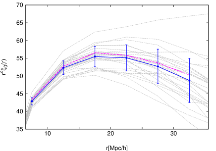
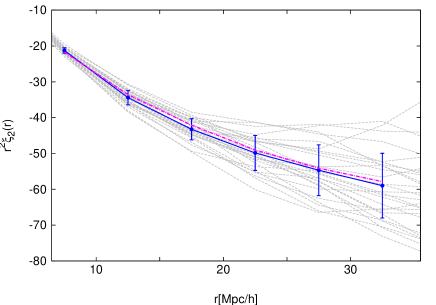
The non-linear model given by Eq. (13) is then integrated to obtain the multipoles according to Eq. (6). So the multipoles of both the measured and the theoretical correlation functions are computed in the same way using the measured correlation function, Eq. (5), and the model correlation function, Eq. (13), respectively, thus minimising any numerical bias. As an example, Fig. 1 shows the comparison between the multipoles computed from the $27$ mock catalogues extracted from the most dense sample with a mass threshold of $M_{cut}=1.1\times 10^{12}\ h^{-1}\ M_{\odot}$, and their best-fit model. We can appreciate the agreement between the model (magenta dot-dashed lines), obtained by fixing all parameters to their best-fit values, and the mean multipoles (blue dots) computed over the $27$ mock catalogues (grey dashed lines). The mean difference between the two is $\sim 5\%$ for the monopole and $\sim 13\%$ for the quadupole.

3.3 Covariance Matrix and Likelihood

We use the $27$ mock catalogues extracted from the BASICC simulation to estimate the covariance matrix. We compute the multipoles of the correlation function for each mock catalogue and construct the covariance matrix as follows:

$$C_{ij}=\frac{1}{N-1}\sum^{N}_{k=1}(\bar{X}_{i}-X^{k}_{i})(\bar{X}_{j}-X^{k}_{j})\;,$$ (15)

where the sum is over the number of mocks $N=27$, and $\mathbf{X}$ is the data vector containing the multipole vectors:

$$\begin{split}\mathbf{X}=&\{\xi^{(1)}_{0},\xi^{(2)}_{0},...,\xi^{(M)}_{0},\xi^{(1)}_{2},\xi^{(2)}_{2},...,\xi^{(M)}_{2}\}\;,\end{split}$$ (16)

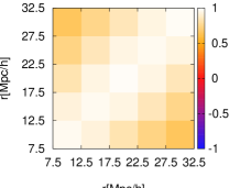
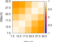
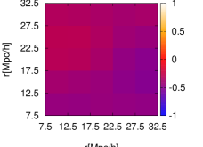
with $M$ being the number of bins, i.e. the dimension of each multipole vector. In particular, $\bar{X}_{i}$ is the mean value over the $27$ catalogues of the $i^{th}$ element of the data vector, while $X^{k}_{i}$ is the value of the $i^{th}$ component of the vector corresponding to the $k^{th}$ mock catalogue. Fig. 2 shows the reduced covariance matrix defined as $\tilde{C}_{i,j}=C_{i,j}/\sqrt{C_{i,i}C_{j,j}}$. We can see that there are significant off-diagonal terms, and a non-negligible covariance between monopole and quadrupole. However, in this work we are going to consider only the diagonal part of the matrix, since this simplification does not affect our final results and reduces numerical noises (see Appendix A for details).

The likelihood is assumed to be proportional to $\exp(-\chi^{2}/2)$ (Press et al., 2007), where $\chi^{2}$ is defined as:

$$\chi^{2}\equiv\sum^{N_{bins}}_{i,j=1}(X_{th,i}-X_{obs,i})C^{-1}_{ij}(X_{th,j}-X_{obs,j})\;;$$ (17)

$N_{bins}$ is the length of the vector X, which is twice the length of each multipole vector. $X_{th}$ is the multipole vector computed from the theoretical correlation function and $X_{obs}$ is the data vector computed from the simulation for each catalogue of Table 2.

Figure 3: Contour plots for $f_{\nu}$ and $b$ derived using the monopole only (blue contours), the quadrupole only (magenta contours) and from their combination (green contours). The results have been obtained from one of the mock catalogues with mass $M_{cut}=1.1\times 10^{12}M_{\odot}\ h^{-1}$ and density $n=3.1\times 10^{-3}h^{3}\ \mathrm{Mpc}^{-3}$. The input values of the simulation, represented by the black dot, are $f_{\nu}=0$ and $b=1.44$. Dark and light ellipses represent $1\sigma$ and $2\sigma$ contours, respectively.

Figure 4: Contour plots for $f_{\nu}$ and $b$ for a single mock catalogue from the samples with $M_{cut}=1.1\times 10^{12}\ M_{\odot}\ h^{-1}$ and density values as in the first column of Table 2. Larger contours correspond to lower density samples. The input values of the simulation, highlighted by the black dot, are recovered within $1\sigma$.

Figure 5: Contour plots for $f_{\nu}$ and $b$ derived considering $f(z)=\Omega^{\gamma}_{m}(z)$ (green contours) and $f(z)\simeq[\Omega_{m}(z)(1-f_{\nu})]^{\gamma}$ (blue contours), using both monopole and quadrupole. The results have been obtained from one of the mock catalogues with mass $M_{cut}=1.1\times 10^{12}M_{\odot}\ h^{-1}$ and density $n=3.1\times 10^{-3}h^{3}\ \mathrm{Mpc}^{-3}$.

3.4 MCMC analysis

We analyse the mock data with a MCMC procedure. We explore a three-dimensional parameter space considering the neutrino mass fraction $f_{\nu}\equiv\Omega_{\nu}/\Omega_{m}$, the halo bias parameter, $b$, and the pairwise velocity dispersion, $\sigma_{12}$. The other cosmological parameters are kept fixed to the input values of the simulations. To investigate the impact of this assumption, we repeated our analysis assuming Plank-like priors for $\Omega_{\rm dm}h^{2}$, $\Omega_{b}h^{2}$ and $A_{s}$. Specifically, we allowed each of these parameters to vary in the ranges $\Delta\Omega_{m}h^{2}=0.001$, $\Delta\Omega_{b}h^{2}=0.00014$, and $\Delta\ln(10^{10}A_{s})=0.023$ (Planck Collaboration, 2015), around the input values of the simulation. As we verified, the effect on our final results is negligible, considering the estimated errors.

The neutrino mass fraction enters the model through the shape of the real-space undistorted correlation function. The bias instead enters the model twice: first, when converting the real-space correlation function of matter into the halo correlation function assuming a linear biasing model, $\xi_{halo}(r)=b^{2}\xi_{m}(r)$, and second in the multipole expansion through the parameter $\beta$, which in our analysis is expressed as $\Omega^{\gamma}_{m}(z)/b(z)$, with $\gamma=0.55$ according to Linder (2005). $\Omega_{m}(z)$ is the input value of the simulation computed at redshift $z=1$ via the equation:

$$\Omega_{m}(z)=\frac{{(1+z)}^{3}\Omega_{m0}}{{(1+z)}^{3}\Omega_{m0}+(1-\Omega_{m0})}\;.$$ (18)

We assume the expression $f(z)=\Omega^{\gamma}_{m}(z)$, neglecting the dependence on $f_{\nu}$ that the growth rate acquires at the scales of interest in this work. Nevertheless, we verified that this does not affect significantly the results, as we will show in the next section.

Once the theoretical correlation function is computed assuming a given set of cosmological parameters, it should be rescaled to the fiducial cosmology used to measure the correlation function, that in our case is the input cosmology of the simulation. This is done by adopting the relation (e.g. see Seo & Eisenstein 2003):

$$\xi^{fid}_{th}(r_{p},\pi)=\xi_{th}\bigg{(}\frac{D_{A}(z)}{D^{fid}_{A}(z)}r_{p},\frac{H^{fid}(z)}{H(z)}\pi\bigg{)}\;,$$ (19)

where $D_{A}(z)$ is the angular diameter distance and $H(z)$ is the Hubble parameter, at redshift $z$. However, in our case this procedure is not necessary since the only varying cosmological parameter is $f_{\nu}$, whereas the total amount of matter $\Omega_{m}$ is held fixed to the input value of the simulation, so that $H(z)$ and $D_{A}(z)$ do not change and there are no geometric distortions to be accounted for.

4 Results

In this section we present our results. First, we compare the cosmological values recovered with the MCMC procedure with the input values of the simulation. Then we show how the errors on $f_{\nu}$ and bias depend on the halo density and the volume covered by the simulation, and on the bias of the considered sample.

Figure 6: Relative errors on the halo bias, $\delta b/b$, as a function of bias, $b$, for different mass (highlighted by different colours) and density samples, as labelled in the panels. The dots represent the mean error over the $27$ mock catalogues, the dashed lines show the scaling formula obtained by fitting our results, Eq. (24).

Figure 7: As Fig. 6 but for the errors on neutrino mass fraction, $\delta f_{\nu}$, as a function of bias, $b$, for different mass and density samples.

4.1 Estimating the neutrino mass fraction

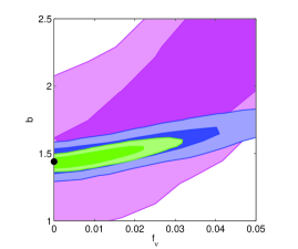
The joint constraints on the neutrino mass fraction, $f_{\nu}$, and bias, $b$, marginalised over the pairwise velocity, $\sigma_{12}$, are shown in Fig. 3. They have been obtained from one mock catalogue of the most dense sample with a mass threshold of $M_{cut}=1.1\times 10^{12}M_{\odot}\ h^{-1}$, using monopole and quadrupole separately (blue and magenta contours, respectively), and monopole and quadrupole together (green contours). Let us notice that the use of both monopole and quadrupole can significantly help to tighten the constraints on both parameters. Indeed, when modelling only the monopole, there is a degeneracy between the halo bias and $f_{\nu}$, since they affect the normalisation of $\xi_{halo}$ in opposite directions. On the other hand, the quadrupole moment, which includes the effects of RSD, can help in breaking this degeneracy, especially for large values of $f_{\nu}$. Therefore, the combination of the first two multipoles of the redshift-space two-point correlation function is crucial to estimate the neutrino mass fraction. We can also notice that the input values of the two parameters, $f_{\nu}=0$ and $b=1.44$, are recovered within $1\sigma$ contours.

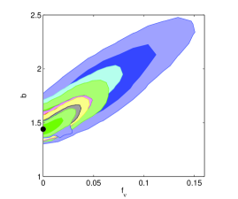
In Fig. 4 we show the $1\sigma$ and $2\sigma$ contours obtained using both monopole and quadrupole for the same mock catalogue of the previous figure, but considering the different density values reported in Table 2. Larger contours correspond to catalogues with lower densities.

Figure 8: Relative errors on bias $\delta b/b$ as a function of density $n$ for different mass (i.e. bias) samples, as labelled in the panels. The dots represent the mean error over the $27$ mock catalogues. The black dashed lines show the scaling formula of Eq. (24). The colour code is the same of the previous figures.

Figure 9: As Fig. 8 but for errors on neutrino mass fraction, $\delta f_{\nu}$, as a function of density, $n$, for different mass (i.e. bias) samples.

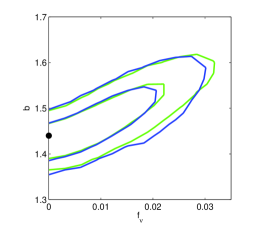
In Fig. 5 we compare the results obtained considering $f(z)=\Omega_{m}^{\gamma}(z)$ (green contours) with the ones obtained assuming $f(z)\simeq[\Omega_{m}(z)(1-f_{\nu})]^{\gamma}$ on the scales of interest in this work, i.e. $k>>k_{FS}$ (as suggested by Kiakotou et al. 2008). The results are very similar, indeed averaging the errors obtained in the two cases, over the $27$ mock catalogues, we find that the difference in the $f_{\nu}$ error is only $\sim 12\%$.

As verified by previous works in the literature, the RSD model used for this analysis is not sufficiently accurate at small non-linear scales, especially for what concerns the quadrupole moment (see e.g. Marulli et al. 2015). Therefore, in order to minimise systematic errors due to theoretical uncertainties, we consider only scales larger than $7.5\ \mathrm{Mpc}/h$, though our final results are not significantly affected by this choice, considering the estimated uncertainties.

4.2 Error dependence on the survey parameters

Having analysed all the samples in Table 2, we can now present the results on the dependence of the errors on three different parameters characterising a survey: bias, density and volume. First, we illustrate the dependence on one single parameter at a time, and then combine these dependencies to provide a fitting formula able to describe the overall behaviour.

4.2.1 Error dependence on bias

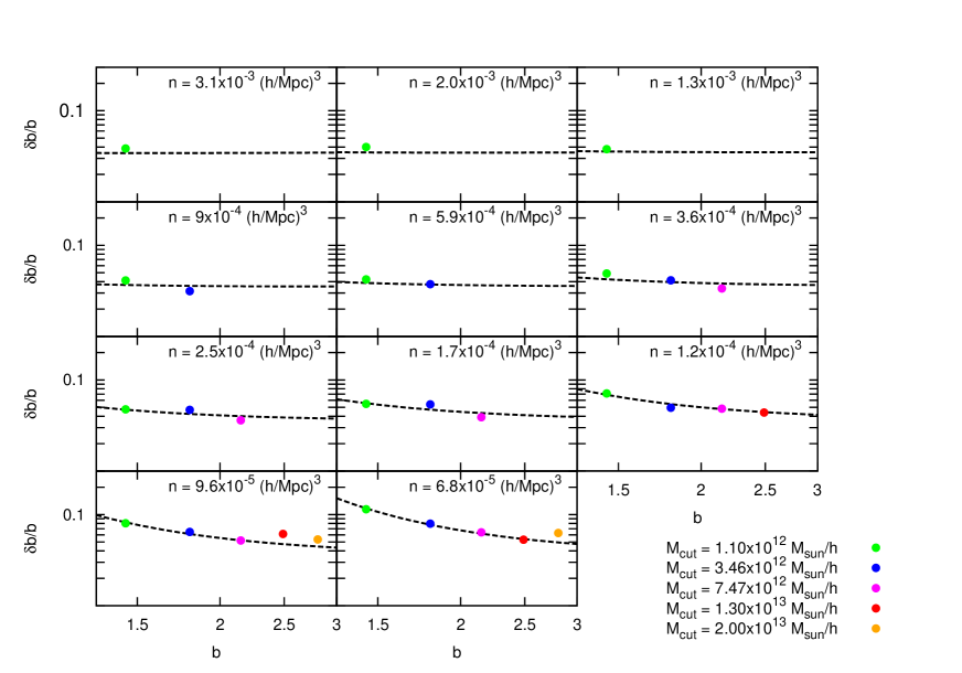
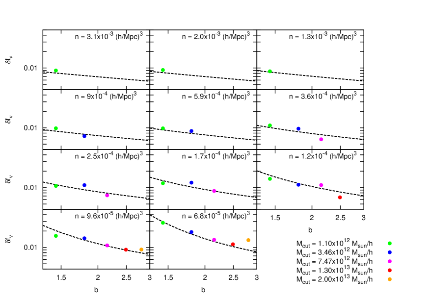
In Figs. 6 and 7, we plot the relative errors on $b$ and $f_{\nu}$, respectively, as a function of bias, in different density bins. For all the samples considered, the volume is taken fixed. The error dependence on the bias is approximately constant in the density range $1.7\times 10^{-4}\ (h/\mathrm{Mpc})^{3}<n<3.1\times 10^{-3}\ (h/\mathrm{Mpc})^{3}$. For densities smaller than $1.7\times 10^{-4}\ (h/\mathrm{Mpc})^{3}$, the error decreases as the bias increases. In the high-density regime, the trend of the error can be described by a power law of the form:

$$\delta x\propto b^{\alpha_{1}}\ .$$ (20)

In the low-density regime, that is below $1.7\times 10^{-4}\ (h/\mathrm{Mpc})^{3}$, the dependence is better described by an exponential decrease:

$$\delta x\propto\exp(1/b^{\alpha_{2}})\ .$$ (21)

These results can be explained as follows. At high densities the errors on $b$ and $f_{\nu}$ are similar for all values of $b$. At low densities, the gain due to a high distortion signal of the low-bias samples is cancelled out by the dilution of the catalogues. Instead, the high-bias samples, which are characterised by a stronger clustering signal and are intrinsically less dense, give a smaller error and then are more suitable when estimating these parameters using the correlation function both in the real and redshift space.

4.2.2 Error dependence on density

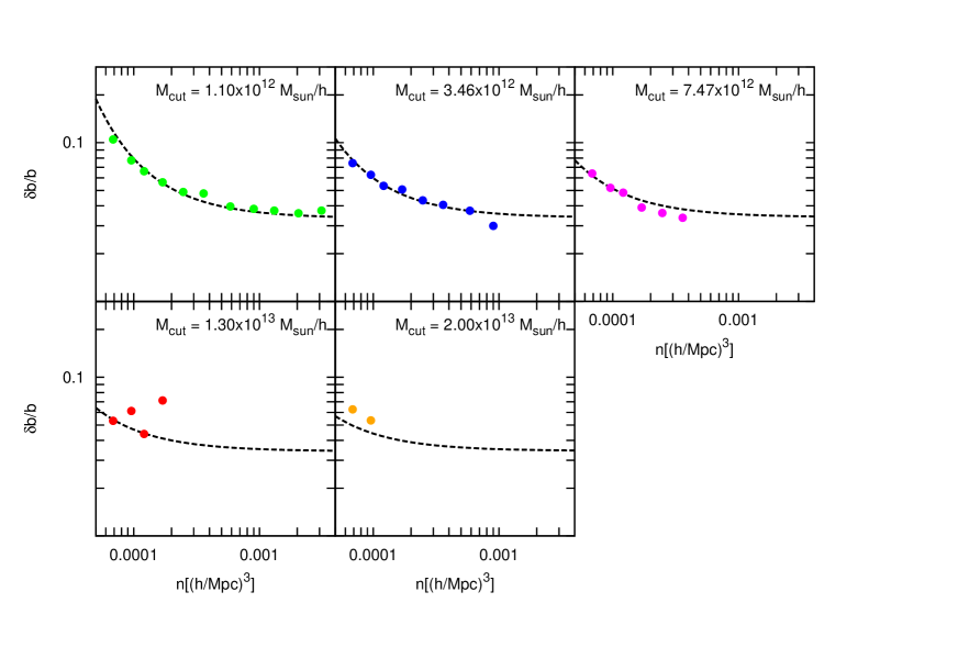
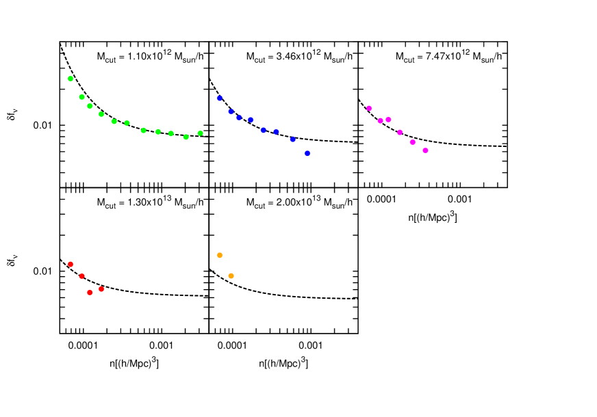
The dependence of the errors on the survey density is shown in Figs. 8 and 9, for $b$ and $f_{\nu}$, respectively. We plot the errors estimated with samples of different bias and density, having fixed the volume. Both the errors decrease exponentially, becoming constant for high values of the density. Indeed, a decrease in the density leads to larger errors, due to the increasing shot noise, whereas moving to higher measurements tend to become cosmic-variance dominated and the errors remain almost constant. This behaviour can be described by an exponential function of the form:

$$\delta x\propto\exp(n_{0}/n)\ ,$$ (22)

where $n_{0}$ is the density value that separates the shot noise regime from the cosmic variance one. We can notice that this exponential decrease depends also on bias, with a flattening of the exponential function for high-bias samples, reflecting what already observed in the previous section. Therefore, it is more appropriate to describe these errors with a function that is a combination of Eq. (21) and Eq. (22):

$$\delta x\propto\exp[n_{0}/(nb^{\alpha_{2}})]\ .$$ (23)

Figure 10: Relative errors on the halo bias, $\delta b/b$ (left panel) and errors on neutrino mass fraction, $\delta f_{\nu}$ (right panel) as a function of volume, for different mass samples (all labelled in the panels). As in the previous figures, the dots represent our measurements and the dashed lines show the fitting formula of Eq. (24).

4.2.3 Error dependence on volume

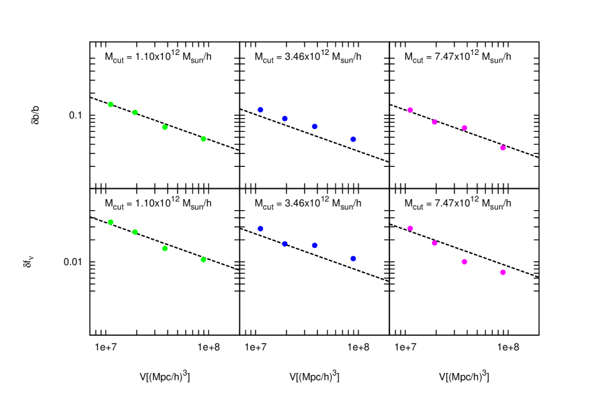
Finally, we illustrate the dependence on volume. We consider $5$ sub-samples of different bias and density, and for each of them we split the cube of the simulation in $N^{3}$ cubes with $N=\{4,5,6\}$, in order to reduce the volume of the catalogues. We apply the same method described before and compute the mean errors for each sub-sample. We find that the errors scale as the inverse of the square root of the volume, irrespective of bias and density, obtaining for $b$ and $f_{\nu}$ the same dependence found by Guzzo et al. (2008) and Bianchi et al. (2012) for $\beta$. The results are shown in Fig. 10, where we plot the measurements from catalogues with different volume and bias values, for a fixed number density.

4.3 Fitting formula for the overall error dependence

According to these considerations, we try to fit the errors with the same functional form proposed by Bianchi et al. (2012) to describe the error on $\beta$:

$$\delta x\approx Cb^{\alpha_{1}}V^{-0.5}\exp\bigg{(}\dfrac{n_{0}}{b^{\alpha_{2}}n}\bigg{)}\;.$$ (24)

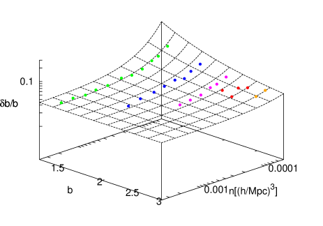
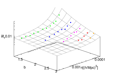
We find that Eq. (24) can describe accurately also the errors on $f_{\nu}$ and $b$. The dashed lines in Figs. 6-10, represent surfaces of Eq. (24). In particular, in Figs. 6 and 7, the dashed lines show Eq. (24) for fixed values of volume $V=8.9\times 10^{7}\ (h^{-1}\ \text{Mpc})^{3}$ and density $n$ (according to the labels of each panel). In Figs. 8 and 9, the volume $V=8.9\times 10^{7}\ (h^{-1}\ \text{Mpc})^{3}$ and the bias $b$ are kept fixed. Finally, the lines in Fig. 10 show the errors given by Eq. (24).

The obtained best-fit parameters for Eq. (24) are: $C=311\ h^{-1.5}$ $\text{Mpc}^{1.5}$, $\alpha_{1}=0.1$ and $\alpha_{2}=1.9$ and $C=72\ h^{-1.5}\ \text{Mpc}^{1.5}$, $\alpha_{1}=0.2$ and $\alpha_{2}=2$ for the errors on $b$ and on $f_{\nu}$, respectively. In both cases we assume $n_{0}=1.7\times 10^{-4}\ h^{3}\ \text{Mpc}^{-3}$, which is roughly the density at which cosmic variance starts to dominate. The errors that we fit are the relative error for $b$, and the absolute error on $f_{\nu}$. Therefore, in the fitting formula of Eq. (24), $\delta x$ should be replaced with $\delta b/b$ and $\delta f_{\nu}$, respectively.

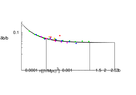
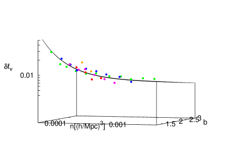
The overall behaviour of both errors is summarised in Fig. 11. In the top panels we plot the error on $b$ and $f_{\nu}$ as a function of density and bias for a fixed volume. The dashed surface represents the fitting function of Eq. (24) with $V=8.9\times 10^{7}\ (h^{-1}\ \text{Mpc})^{3}$. The bottom panels show the same points, but suitably oriented to highlight the agreement with the fitting function of Eq. (24).

5 Summary and Discussion

We have performed an extended analysis to forecast the statistical errors of the neutrino mass fraction and the bias parameter exploiting the correlation function in the redshift space. We have measured the multipoles of the correlation function in bins of $5\ \mathrm{Mpc}\ h^{-1}$, up to a scale of $35\ \mathrm{Mpc}\ h^{-1}$, from mock data extracted from the halo catalogues of the BASICC simulation at $z=1$. The halo catalogues have been selected in order to have different values of bias, density and volume, that are three fundamental parameters used to describe a redshift survey.

The mock data have been analysed using an MCMC likelihood method with $f_{\nu}$, $b$ and $\sigma_{12}$ as free parameters, fixing all other parameters to the input value of the simulation. We have presented the results concerning only $f_{\nu}$ and $b$, considering $\sigma_{12}$ just as a nuisance parameter needed to take into account the effect of non-linear motions. The best-fit values for these two parameters are in agreement with the input values of the simulation within $1\sigma$ for each considered sample.

The scale-dependent suppression in the power spectrum induced by massive neutrinos would allow to constrain separately $f_{\nu}$ and $b$. However, this effect is quite small, and it is difficult to extract these constraints from the real-space clustering alone, due to current measurement uncertainties. On the other hand, they can be efficiently extracted from the redshift-space monopole of the correlation function, as shown in Fig. 1. Indeed, as explained in §3.4, while $f_{\nu}$ enters the model only through the shape of the real-space undistorted correlation function, the bias enters the model twice, both in the real-space correlation function of matter and in the multipole expansion through $\beta$. The quadrupole multipole has larger errors with respect to the monopole. Still it can be exploited to improve our measurements as the constrain direction is slightly different (see Fig. 1 and Eqs. 10). Thus, as we have shown, the use of both monopole and quadrupole together can help in breaking the degeneracy between the halo bias and $f_{\nu}$.

For what concerns the error trend as a function of density, volume and bias, we found that our measurements are fitted to a good approximation by the scaling formula given in Eq. (24) for both $\delta b/b$ and $f_{\nu}$.

A crucial point in this work is represented by the covariance matrix. We have decided to use only its diagonal part. Though the off-diagonal elements are not negligible, they are also very noisy due to the small number of mock catalogues available, compared to the number of bins used to compute the correlation function. However, the results presented in this work are not biased by the use of the diagonal matrix. As shown in the appendix, the full covariance matrix introduces just a slight shift in the fitting function, and it does not alter its form.

Some aspects still need to be investigated. An improvement of the fitting formula including a redshift dependence would be desirable. Moreover, having a larger number of simulations with different $\sigma_{8}$ can be useful to check if the variation of this parameter could affect the error on $f_{\nu}$. Finally, according to recent works (Castorina et al. 2014; Villaescusa-Navarro et al. 2015), it would be better to consider a linear bias defined as $b^{2}\equiv\xi_{halo}/\xi_{cdm}$. However, when considering small neutrino masses, the error caused by the assumption of a linear bias defined in terms of $\xi_{m}$, instead of $\xi_{cdm}$, is negligible considering the estimated errors of this analysis (see Castorina et al. (2015) for details about the effect of this choice on growth rate estimations).

Table 3: Forecast errors on neutrino mass fraction obtained with the fitting function given by Eq. (24) for some future galaxy surveys, assuming a bias factor $=1$.

	$V[(\text{Mpc}/h)^{3}]$	$n\ [h^{3}\ \text{Mpc}^{-3}]$	$\delta f_{\nu}$
Euclid	$1.6\times 10^{10}$	$1\times 10^{-3}$	$6.7\times 10^{-4}$
WFIRST	$1\times 10^{10}$	$1.3\times 10^{-3}$	$2\times 10^{-4}$
DESI	$4\times 10^{10}$	$4.2\times 10^{-4}$	$4\times 10^{-4}$

Regardless these still open issues, the presented fitting formula can be used to forecast the precision reachable in measuring the neutrino mass fraction with forthcoming redshift surveys. Recent constraints on neutrino mass came from different cosmological probes. For example, the latest Planck results (Planck Collaboration, 2015) put an upper limit on the sum of neutrino masses $\sum m_{\nu}<0.23\ \mathrm{eV}$, and, in combination with LSS surveys, the following constraints have been obtained: $\sum m_{\nu}<0.18\ \mathrm{eV}$ (Riemer-Sørensen et al., 2010), $\sum m_{\nu}<0.29\ \mathrm{eV}$ (Xia et al., 2012) and $\sum m_{\nu}=0.35\pm 0.10\ \mathrm{eV}$ (Beutler et al., 2014). If we consider that a Euclid-like survey should be able to cover a volume of $V\approx 1.6\times 10^{10}(\mathrm{Mpc}/h)^{3}$, targeting a galaxy sample with bias $b\approx 1.3$ and density $\approx 10^{-3}(h/\mathrm{Mpc})^{3}$, the neutrino mass fraction can be measured with a precision of $\approx 6.7\times 10^{-4}$. This value translates into an accuracy of $\delta\left(\sum m_{\nu}\right)\approx 0.0081\ \mathrm{eV}$, smaller than the one quoted into the Euclid Red Book (Laureijs et al., 2011), obtained with the Fisher Matrix method from BAO measurements. This is mainly due to the fact that our predictions have been derived using very different probes and methodology, but most of all because we kept fixed many of the relevant cosmological parameters such as, for example, $\Omega_{m}$ and the initial scalar amplitude of the power spectrum (see e.g. Carbone et al., 2011). Predictions for other surveys are reported in Table 3. Overall, our analysis confirms that the two-point correlation function in redshift space provides a promising probe in the quest for neutrino mass.

Figure 11: Top panels: relative errors on the halo bias, $\delta b/b$ (left) and errors on neutrino mass fraction, $\delta f_{\nu}$ (right), as a function of density, $n$, and bias, $b$, over-plotted on the surface described by the fitting formula of Eq. (24) for a fixed volume $V=8.9\times 10^{7}\ (h^{-1}\ \text{Mpc})^{3}$. Bottom panels: the same as the ones in top panels, except for the fact that the axes are oriented in order to highlight the agreement between our measurements and the fitting function. The colour code is the same of the previous figures.

Appendix A Assessing the validity of the covariance matrix

The results presented in this work have been obtained considering only the diagonal elements of the covariance matrices. Here we briefly review the reasons that brought us to this choice. In order to test the effects introduced by different covariance matrix assumptions, we repeat our analysis using three different matrices, the diagonal matrix, the full matrix and the smoothed matrix, the last one obtained with a smoothing algorithm that follows the approach presented in Chuang & Wang (2012). Specifically, the latter algorithm exploits the fact that the diagonal elements of the covariance matrix are larger than the first off-diagonal elements, than in turn are larger than all other elements (see Fig. 2). Therefore, we consider the vector made up by the diagonal elements only and average each of them using the two nearby elements, according to the formula:

$$\tilde{C}(i,i)=(1-p)C(i,i)+\\ p\left[C(i+1,i+1)+C(i-1,i-1)\right]/2,$$ (25)

where $p$ is a weight. If one of the two nearby elements is not present (i.e. when we consider the first and the last element of the vector), then $\tilde{C}(i,i)=C(i,i)$. The same algorithm is applied to the first off-diagonal elements, while the “generic” elements of the covariance matrix are averaged using all the nearby elements:

$$\tilde{C}(i,j)=(1-p)C(i,j)+\\ \frac{p}{m}\cdot\begin{bmatrix}C(i+1,j)+C(i-1,j)+\\ C(i,j+1)+C(i,j-1)+\\ C(i+1,j+1)+C(i-1,j-1)+\\ C(i+1,j-1)+C(i+1,j-1)\end{bmatrix},$$ (26)

where $m$ is the number of nearby elements used in the averaging procedure. For all the matrix elements we used $p=0.01$. As verified, this smoothing procedure helps to alleviate some of the numerical problems related to the matrix noise, though it does not work properly for all cases considered.

Figure 12: Relative error on the distortion parameter, $\delta\beta/\beta$ (upper panel), and bias, $\delta b/b$ (lower panel), as a function of density, $n$, obtained analysing the mock data with $\beta$ and $b$ as free parameters. The dots represent the MCMC error averaged over the $27$ mock catalogues extracted from the most dense sample with $M_{cut}=1.1\times 10^{12}\ h^{-1}\ M_{\odot}$, obtained using the diagonal matrix (blue dashed lines), the full matrix (green dotted lines) and the smoothed matrix (red dot-dashed lines).

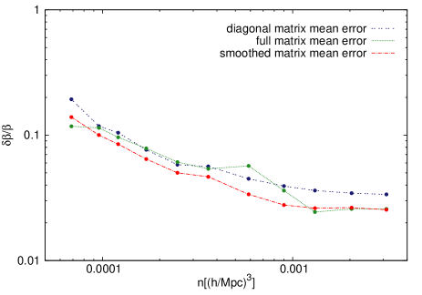
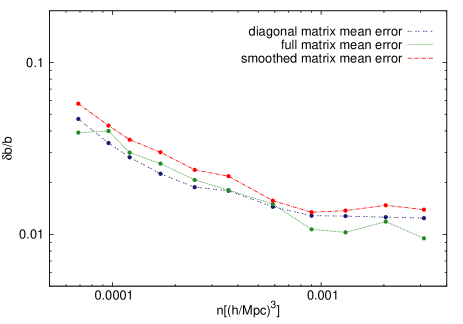
For these tests, we consider the simple case where the only free parameters of the MCMC analysis are the distortion parameter, $\beta$, and the bias, $b$. We choose this limited parameter space in order to speed up the computation. Fig. 12 shows the errors on $\beta$ and $b$ as a function of density, obtained with the diagonal matrix (blue dashed lines), the full matrix (green dotted lines) and the smoothed matrix (magenta dot-dashed lines). As it can be noted, the shape of the curves is quite similar, while the normalisation is slightly different. For instance, the differences between the errors obtained with the diagonal and the full covariance matrix are $\sim 5\%$ for $\beta$ and $\sim 2\%$ for $b$. However, the small number of mock catalogues available to construct the covariance matrices, relative to the number of bins analysed, does not allow us to get robust results Hartlap et al. (2007). These reasonings, together with the fact that using the diagonal matrix we get a less scattered trend for the errors in all the cases considered, lead us to neglect the non-diagonal elements of the covariances.

References

- Angulo et al. (2008) Angulo R. E., Baugh C. M., Frenk C. S., Lacey C. G., 2008, MNRAS, 383, 755
- Beutler et al. (2014) Beutler, F., Saito, S., Brownstein, J. R., Chuang, C. H., Cuesta, A. J., Percival, W. J., Ross, A. J., Ross, N. P., Schneider, D. P., Samushia, L., Sánchez, A. G., Seo, H. J., Tinker, J. L.; Wagner, C., Weaver, B. A., 2014, MNRAS, 444, 3501
- Bianchi et al. (2012) Bianchi D., Guzzo L., Branchini E., Majerotto E., de la Torre S., Marulli F., Moscardini L., Angulo R. E., 2012, MNRAS 427, 2420
- Beringer et al. (2012) Beringer J. et al. [Particle Data Group Collaboration], 2012, Phys. Rev. D 86, 010001
- Carbone et al. (2011) Carbone, Carmelita; Verde, Licia; Wang, Yun; Cimatti, Andrea, 2011, JCAP 03, 030
- Castorina et al. (2015) Castorina, Emanuele; Carbone, Carmelita; Bel, Julien; Sefusatti, Emiliano; Dolag, Klaus, 2015, JCAP 07, 043
- Castorina et al. (2014) Castorina, E., Sefusatti, E., Sheth, R. K., Villaescusa-Navarro, F., Viel, M., 2014, JCAP 02, 049
- Chuang & Wang (2012) Chuang C.H., Wang Y., 2012, MNRAS, 426, 226
- Davis & Peebles (1983) Davis M., Peebles P. J. E., 1983, ApJ, 267, 465
- Davis et al. (1985) Davis M., Efstathiou G., Frenk C. S., White S. D. M., 1985, ApJ, 292, 371
- Dunkley et al. (2009) Dunkley, J. et al. [WMAP Collaboration], 2009, Astrophys. J. Suppl. 180, 306
- Elgarøy & Lahav (2005) Elgarøy, Ø., Lahav, O., 2005, New Journal of Physics, 7, 61
- Fisher et al. (1994) Fisher K. B., Davis M., Strauss M. A., Yahil A., Huchra J. P., 1994, MNRAS, 267, 927
- Guzzo et al. (2008) Guzzo L., et al., 2008, Nature, 451, 541
- Hamilton (1992) Hamilton A. J. S., 1992, ApJ, 385, L5
- Hamilton (1998) Hamilton A. J. S., 1998, ASSL, 231, 185
- Hartlap et al. (2007) Hartlap, J., Simon, P., Schneider, P., 2007, A&A, 464, 399
- Hinshaw et al. (2009) Hinshaw, G. et al. [WMAP Collaboration], 2009, Astrophys. J. Suppl. 180, 225
- Hinshaw et al. (2013) Hinshaw, G. et al. [WMAP Collaboration], 2013, Astrophys. J. Suppl. 208, 19
- Hu et al. (1998) Hu, W., Eisenstein, D. J., Tegmark, M., 1998, Phys. Rev. Lett., 80, 5255
- Kaiser (1987) Kaiser N., 1987, MNRAS, 227, 1
- Kiakotou et al. (2008) Kiakotou, A., Elgarøy, Ø., Lahav, O., 2008, Phys. Rev. D, 77, 063005
- Kofman & Starobinskij (1985) Kofman, L., Starobinskij, A. A., 1985, Soviet Astronomy Letters, 11, 271
- Komatsu et al. (2011) Komatsu E. et al. [WMAP Collaboration], 2011, Astrophys. J. Suppl. 192, 18
- Ichiki et al. (2009) Ichiki K., Takada M., Takahashi T., 2009, Phys. Rev. D 79, 023520
- Landy & Szalay (1993) Landy S. D., Szalay A. S., 1993, ApJ, 412, 64
- Laureijs et al. (2011) Laureijs R., et al., 2011, arXiv, arXiv:1110.3193
- Lesgourgues & Pastor (2014) Lesgourgues J., Pastor S., 2014, New Journal of Physics 16, 6
- Lewis&Bridle (2002) Lewis, A., Bridle, S., 2002, Phys. Rev. D, 66, 10
- Lewis et al. (2000) Lewis, A., Challinor, A., Lasenby, A., 2000, ApJ, 538, 473
- Linder (2005) Linder, E. V., 2005, Phys. Rev. D, 72, 4
- Marulli et al. (2011) Marulli, F., Carbone, C., Viel, M., Moscardini, L., Cimatti, A., 2011, MNRAS, 418, 346
- Marulli et al. (2012) Marulli, F., Bianchi, D., Branchini, E., Guzzo, L., Moscardini, L., Angulo, R. E., 2012, MNRAS, 426, 2566
- Marulli et al. (2015) Marulli, F., Veropalumbo, A., Moscardini, L., Cimatti, A., Dolag, K., arXiv:1505.01170
- Marulli et al. (2015b) Marulli, F., Veropalumbo, A., & Moresco, M. 2015, arXiv:1511.00012
- Peacock (1999) Peacock J. A., 1999, Cosmological Physics, Cambridge Univ. Press, Cambridge
- Planck Collaboration (2015) Planck 2015 results. XIII. Cosmological parameters, arXiv:1502.01589
- Press et al. (2007) Press W. H., Teukolsky S. A., Vetterling W. T., Flannery B. P., 2007, Numerical Recipes: The Art of Scientific Computing, Third Edition
- Reid et al. (2010) Reid B. A., Verde L., Jimenez R., Mena O., 2010, JCAP, 01, 003
- Riemer-Sørensen et al. (2010) Riemer-Sørensen, S., Parkinson, D.; Davis, T. M., 2014, Phys. Rev. D, 89, 10, 103505
- Sachs & Wolfe (1967) Sachs, R. K., Wolfe, A. M., 1967, ApJ, 147, 73
- Saito et al. (2011) Saito S., Takada M., Taruya A., 2011, Phys. Rev. D 83, 043529
- Sánchez et al. (2012) Sánchez A. G. et al., 2012, MNRAS 425, 415
- Seljak et al. (2006) Seljak U., Slosar A. and McDonald P., 2006, JCAP 0610, 014
- Seo & Eisenstein (2003) Seo H.-J., Eisenstein D. J., 2003, ApJ, 598, 720
- Tinker et al. (2010) Tinker J. L., Robertson B. E., Kravtsov A. V., Klypin A., Warren M. S., Yepes G., Gottlöber S., 2010, ApJ, 724, 878
- Thomas et al. (2010) Thomas S. A., Abdalla F. B., Lahav O., 2010, Phys. Rev. Lett. 105, 031301
- Villaescusa-Navarro et al. (2015) Villaescusa-Navarro, F., Bull, P., Viel, M.
- Villaescusa-Navarro et al. (2015) Villaescusa-Navarro, F., Marulli, F., Viel, M., et al. 2014, JCAP, 3, 011
- Wang et al. (2005) Wang, S., Haiman, Z., Hu, W., Khoury, J., May, M., 2005, Phys. Rev. Lett., 95, 011302
- Xia et al. (2012) Xia, J. Q., Granett, B. R., Viel, M., Bird, S., Guzzo, L., Haehnelt, M. G., Coupon, J., McCracken, H. J.; Mellier, Y., 2012, JCAP, 06, 010