Long-range Response in AC Electricity Grids
Abstract
Local changes in the topology of electricity grids can cause overloads far away from the disturbance Witthaut2013 , making the prediction of the robustness against changes in the topology – for example caused by power outages or grid extensions – a challenging task. The impact of single-line additions on the long-range response of DC electricity grids has recently been studied Labavic2014 . By solving the real part of the static AC load flow equations, we conduct a similar investigation for AC grids. In a regular 2D grid graph with cyclic boundary conditions, we find a power law decay for the change of power flow as a function of distance to the disturbance over a wide range of distances. The power exponent increases and saturates for large system sizes. By applying the same analysis to the German transmission grid topology, we show that also in real-world topologies a long-ranged response can be found.
pacs:
88.80.H-, 88.80.hm, 88.80.hh, 84.70.+p.Power grids reliably provide eletrical power to billions of individuals. For example, in Germany the average outage time experienced by a consumer in 2006 was 20 minutes and continued to decrease in the last decade to 12.5 minutes in 2014 bundesnetzagentur . Still, the energy transition towards an increased supply of decentralized renewable energy raises concerns that the change from the previously centralised power production with unidirectional power flow towards a decentralised electrical power system with bidirectional flow might be harmful for the stability of electricity grids. In a conventional energy grid, the largest consumers (industry) as well as the largest generators usually consist of large rotating masses, so small perturbations are sufficiently damped. As of the energy transition towards an increasingly decentral power generation, generators that do not possess this kind of buffer of electrical energy in form of inertia – namely photovoltaic cells – produce an increasing share of the energy supply. Disturbances and power outages might spread more easily in highly connected grids and cause nonlocal disturbances, which may cause larger instabilities of the entire grid. Therefore, it is essential to get a better understanding of the physical mechanisms leading to nonlocal disturbances and how their spreading depends on the connectivity and topology of the grid.
In a previous work, the long-range response to the addition of a single transmission line has been studied for the case of a DC grid including losses by Joule heating Labavic2014 . It has been demonstrated that the absolute change of transmitted power as function of the distance to the perturbation follows a power law. Real power transmission grids usually use three-phasic alternating current (AC) Heuck2013 . Hence, we are going to perform a similar analysis for AC networks.

An electrical power transmission system can formally be described as a multigraph that consists of nodes (substations) and edges (transmission lines), where is the set of all nodes and the set of all edges of . The network model gains its physical meaning by defining appropriate node and edge attributes. Starting from the Kirchhoff’s laws and Ohm’s law, it is straighforward to write down the steady state power flow equations for a three-phase AC network,
| (1) |
where the three alternating currents of the same frequency are phase-shifted by 120 degrees. Here, is the net generated power entering the network at node (negative for a consumer) and is the terminal voltage of the “machine” connected at node . is the admittance of the transmission line conj . For an arbitrary transmission line in an (one-phasic) AC network, the labeling is illustrated in Fig. 1.
If we restrict ourselves to a purely inductive grid,
| (2) |
we can assume sinusoidal voltages with a constant magnitude Kettemann2015 ,
| (3) |
with phase angles . Thus, only the phase difference between adjacent nodes gives rise to an electrical current. We are looking for steady states with constant grid frequency (e.g. ). The power capacity of a transmission line (a set of three wires) is given by
| (4) |
So the power flow equations (1) become
| (5) |
The real part gives the balance of the active power flow,
| (6) |
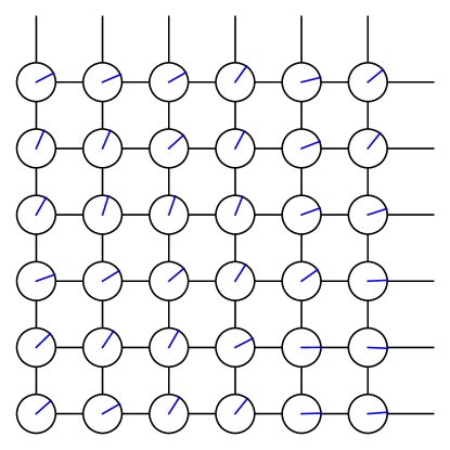
which determines the phases at all nodes for the given load distribution . The imaginary part of Eq. (5) gives the balance of the reactive power . For the constant voltage amplitudes considered in this article, the active power equations determine the phases which also fix the reactive power at all nodes . Eq. 6 can also be derived from the established synchronous motor model (swing equation) Filatrella2008 ; Nishikawa2015 by setting all time-dependent terms to zero.
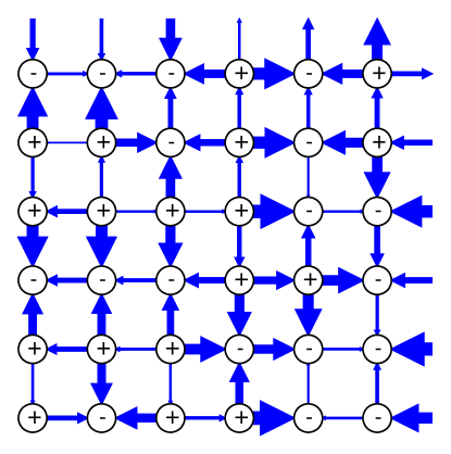
If there exists a stationary solution for the chosen system parameters, it can easily be found using a standard root-finding algorithm root ; multistability (see Fig. 2a for an example phase distribution). Given a solution for the phase distribution , the transmitted power from node to node is given by
| (7) |
as plotted in Fig. 2b, where the thickness of the arrows is proportional to .
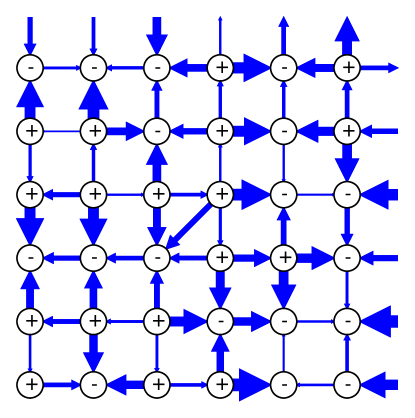
Then we add a single line to the graph and calculate the modified transmitted powers (see Fig. 3a). We calculate the difference and study the average absolute difference of all edges as a function of their distance to the added line (see Fig. 3b). The average covers all edges with the same distance to the added line as well as an ensemble average over random load distributions .
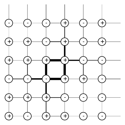
We first consider a regular 2D grid graph of linear size with cyclic boundary conditions, so the system size (number of nodes) is given by . In this graph it is particularly simple to define a measure for the distance between two edges, by counting the number of edges that have to be passed (shortest path), as illustrated in Fig. 4. We further consider a binary distribution for the nodal net generated power , where nodes with are regarded as generators and nodes with as consumers. We set the power capacity of all lines to , so we can note down all power quantities in units of . In order to find a stable solution, the condition must be fulfilled at all times, which rules out the possibility of odd linear system sizes .
In order to precisely control the amount of randomness in the system, we use the following procedure to generate a random distribution of the : We start from a periodic arrangement of generators and consumers antiferro and divide the graph into two subgraphs, one carrying all generators and the other all consumers. Then, different nodes are chosen randomly from each subgraph, forming generator-consumer pairs. Finally, each of these generator-consumer pairs is swapped. By generating a permutation of the periodic arrangement in this way, it is ensured that no node is swapped twice, and the degree of randomness can precisely be specified as
| (8) |
depending on the number of swapped generator-consumer pairs . The reasoning here is that after permutations, the periodic arrangement is reached again, but with all original consumers and generators swapped. If only half as many permutations are done, , the state should be the furthest away from one of the two possible periodic arrangements and thus correspond to maximum randomness. There is a finite number of possible realizations , given by the ensemble size
| (9) |
which is large compared to , even for the smallest considered system sizes.
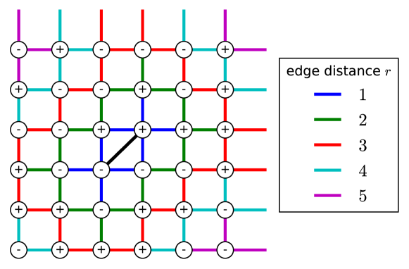
To study the long-range response of the grid to the added transmission line, we classify all edges of the graph by their distance to the added edge by counting the number of edges that link the considered edge to the added edge (see Fig. 4 for an illustration). We average the change in the amplitude of the transmitted power over all edges with the same distance to the added line, and perform an ensemble average over realizations with the same randomness . Realizations for which no steady state solution can be found are skipped. This happens in particular if the transmitted power is exceeding the capacity of at least one transmission line , so that Eq. (7) cannot be fulfilled. For the square grid, the power capacity has to exceed the critical value in order to obtain a steady state power flow at all kc . Since for a random arrangement of , clusters of generators or consumers can occur with total power , the lines connected to these clusters can be overloaded even if the power capacity exceeds the critical value , and no steady state solution is found. Thus, only a certain subset of realizations leads to a solution for the phase distribution .
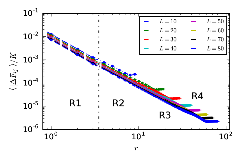
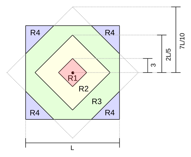
has been calculated for different linear system sizes and plotted on a double-logarithmic scale in Fig. 5. Up to a certain distance (saturation distance), is a steadily decreasing function of . The value is found to depend linearly on the linear system size , roughly as . For distances exceeding (region R4), the data saturates, or even a small increase is noticable, which is caused by the cyclic boundary conditions as confirmed in a comparative analysis. For distances we are able to identify two regimes R1 () and R2 () that both show a power-law-like behavior of , but with different power exponents . Beyond R2 (for about ), there is a region where the data is closer to an exponential law (region R3), as the semi-logarithmical plot in Fig. 9 shows. The four regions of the 2D grid with different dependencies of on are sketched in Fig. 6.
For the regimes R1 and R2, we fit the data to a power law, using the fit model
| (10) |
where is either 1 (regime R1) or 2 (regime R2). The fit results for regime R2 and are listed in Tab. 1 (see the appendix for more complete list of fit results). To assess the quality of the fit, we compute the statistic and the goodness of fit probability gof . For the error bars, a confidence level is considered confidence .
| 20 | 4 | 2 | ||||
| 30 | 8 | 6 | ||||
| 40 | 12 | 10 | ||||
| 50 | 16 | 14 | ||||
| 60 | 20 | 18 | ||||
| 70 | 24 | 22 | ||||
| 80 | 28 | 26 |
Due to the small number of data points () in the small distance regime R1, the fit quality in regime R1 cannot be expected to be acceptable. But also in regime R2, where – depending on the system size – a much larger number of data points is accessible, the values for the goodness of fit probability gof are very low, indicating that the data cannot be described by a pure power law, despite the obvious qualitative indications. On the one hand, this is due to the crossover from one region to another. On the other hand, in many cases the data seems to contain small oscillations around the fitted power law, a behavior our fit model is not able to cover. Nevertheless, we find clear evidence that the response of the power flow in an AC power transmission grid to a local modification of the topology is of long-ranged nature, decaying mainly with a power law with distance .
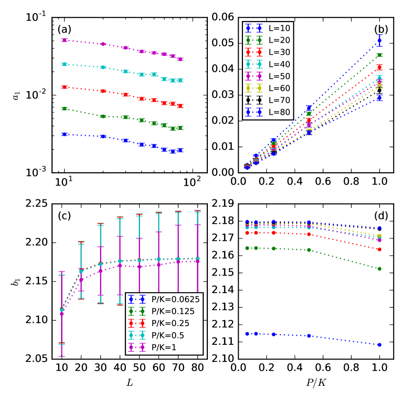
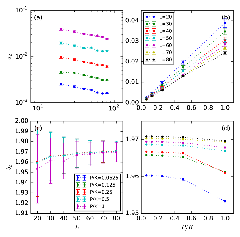
In Figs. 7 and 8, we analyze the dependence of the fit parameters , (regime R1) and , (regime R2) on the linear system size and the power transmission capacity ratio . The data suggests a saturation of the power exponents and in the limit of large system sizes. We find the largest in R1 and in R2, for a linear system size of , when the power is set to . We also detect a clear dependence on the ratio : and both show a decrease when is increased, leading to an even more pronounced long-range behavior. This decrease is expected, since the closer the electricity grid is driven to its maximal transmission capacity (some critical ratio that depends on the topology and load distribution), the smaller are the allowed changes when adding the transmission line.
In contrast to the power exponents , the preexponentials in Eq. (10) increase linearly with , as shown in Figs. 7b and 8b. This behavior is expected as well, as the addition of a transmission line with power capacity will lead to a redistribution of the power flow in proportion to the generated power , so that is expected on average. Further, and decrease monotonically, roughly following a power law, with linear system size (see double logarithmic plots in Figs. 7a and 8a).
For larger distances, beyond the region R2, no power law behavior can be observed anymore. Ignoring also here a certain inaccuracy due to crossover effects and oscillating data, one can however roughly identify an exponential decay in region R3, as illustrated by the semi-logarithmic representation of the data in Fig. 9. The data in regime R3, stretching from to , is fitted to an exponential decay law,
| (11) |
The resulting fit parameters are listed in the appendix in Tab. 5.
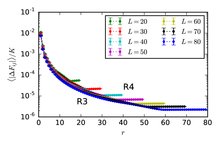
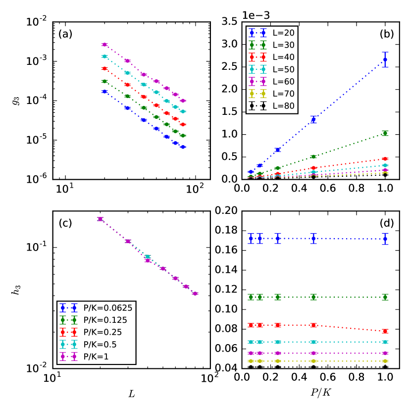
The dependence of the fit parameters and on the linear system size and the power ratio are visualized in Fig. 10. The decay of the preexponential with increasing linear system size is even better described by a power law as that of the fit parameters and in regions R1 and R2 (see Fig. 10a), and increases linearly with increasing , just as and (see Fig. 10b). The exponent decreases as a power law with increasing as well, but stays constant for increasing (see Figs. 10c+d).
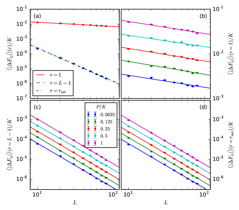
We also analyze the value of directly as function of linear system size for the smallest distance , the largest distance and at the value , where starts to saturate, as shown in Fig. 11. The dependence on is qualitatively following a power law, , in accordance with the behavior of the parameters , and . The fit results are summarized in Tab. 2 and visualized in Fig. 11, setting . We find a different power exponent in the small distance regime at than in the limit of large distances . The low fit quality again shows that the data does not follow a pure power law (with ) underestimated .
Having verified the long-range response of local grid modifications in AC electricity grids, a comparison of the results to an earlier study considering long-range response in DC grids Labavic2014 is in place, where a power capacity ratio of has been used. In the DC case, also two power-law regimes R1 and R2 have been found, and also there, the power exponent is larger than . The absolute values of the exponents are however different in the two studies: In the short distance regime (R1), for a linear system size of , a value of is found Labavic2014 , while for the AC model and , we find . In the medium distance regime (R2), the DC study finds Labavic2014 , while we find a remarkably different value of .
| 8 | ||||||
|---|---|---|---|---|---|---|
| 8 | ||||||
| 8 | ||||||
| 8 | ||||||
| 8 | ||||||
| 8 | ||||||
| 8 | ||||||
| 8 | ||||||
| 8 | ||||||
| 8 | ||||||
| 8 | ||||||
| 8 | ||||||
| 8 | ||||||
| 8 | ||||||
| 8 |
In order to move towards more realistic grid topologies, we also study the effect of single line additions in a model for the German transmission grid (220 kV and 380 kV). The model is based on open data provided by the SciGRID project scigrid and forms a multigraph, which means that some node pairs are connected by more than one transmission line. Filtering the largest connected component, the model grid contains 467 nodes and 755 edges (see Fig. 12). The graph as such is 1-connected, which means it suffices to remove one node to render the graph disconnected. The grid contains stubs and also larger subgraphs that are connected by only one node to the rest of the grid (cut nodes). It is immediately clear that a perturbation that changes the flow of power through the network cannot spread across such cut nodes into another 2-connected subgraph, as there exists no alternative path for the power to be rerouted along. For the sake of this study, it thus makes sense to filter only the largest 2-connected component of the grid, which contains only 260 nodes and 479 edges (see Fig. 12).
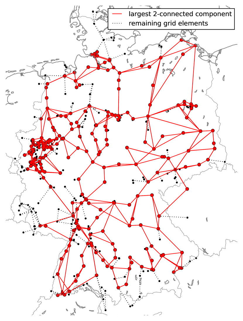
Despite topology, we make the same assumptions as before: We use a constant power capacity (for the lines of both voltage levels) and consider a binary load distribution at the nodes. The distance is measured by counting the edges on the shortest path to the added transmission line which should be a reasonable approach as long as a constant line capacity is used.
The most important difference to the cyclic 2D grid is that the resulting response behavior will depend on the location of the added line. As before in the 2D square grid, we only consider adding single lines that connect next-nearest neighbors (nodes that are two edges apart). Furthermore, we limit their length to 208 km, which is the length of the longest line that exists in the unperturbed grid. There exist 880 candidates for adding a line fulfilling these conditions. For each candidate , we again calculate , shown in Fig. 13.
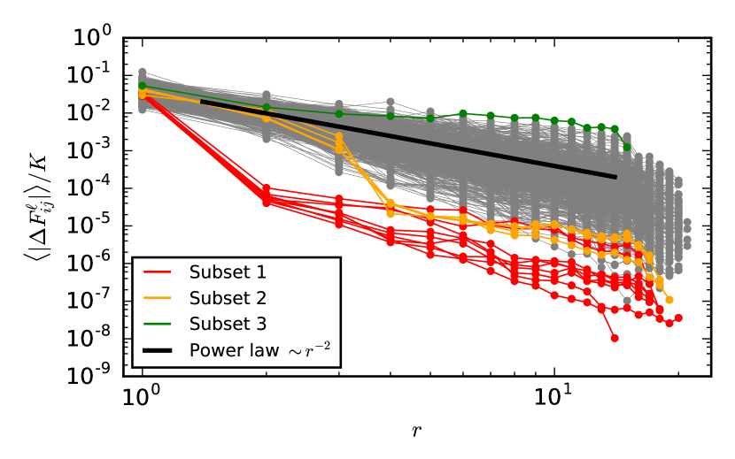
The eccentricity of each added edge can directly be read off from Fig. 13 as the maximal value of of each line. The highest eccentricity observed is 21, which can only be realized for some edges that are added close to the boundaries of the graph (the diameter of the unperturbed graph is also 21). For the majority of added lines, we find a long-range response for similar to the 2D grid, roughly conglomerating around a power law decay with power exponent of about 2 (compare the black line in Fig. 13). However, none of the curves follows a pure power law. Depending on the specific line added to the grid, the exponent can be appreciably smaller or larger than 2, and the decay rate also depends on the distance . The magnitude of varies considerably among the added lines, and sometimes shows sudden drops by orders of magnitude at a certain distance , corresponding to a large decay rate. In the following, we try to identify some noticable subsets of the curves, trying to relate their characteristic long-range response behavior to the local grid structure in the vicinity of each corresponding added line.
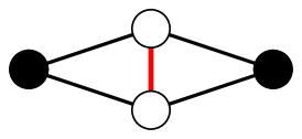
The first considered subset of added lines corresponds to the nine red curves in Fig. 13 that drop quickly by two orders of magnitude already at a distance of . It turns out that all the lines belonging to this subset possess the same local grid structure in its vicinity, which is illustrated by the sketch in Fig. 14. The added line (marked in red) perpendicularly connects two parallel routes of transmission lines that have the same end points A and B that are the only nodes connected to the rest of the network. It is clear that in this case, the power flow in the rest of the network will be altered only marginally by the addition of the line, as it cannot contribute much to the transmission capacity of the double route from A to B. Apparently, it can only lead to an appreciable change of load in the lines directly adjacent to it.
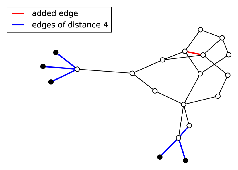
The second subset we consider contains the four curves that show a sudden drop at a distance of , by over one order of magnitude (orange lines in Fig. 13). Here, we cannot identify a common local grid structure anymore like in the example above. However, the local grid structure around the added lines still share some similarities: In all three cases, the line is added inside a subgraph with a radius of about 3, that is only weakly connected to the rest of the grid by only a small number of nodes (two or more). Edges of distance 4 lie just beyond these connecting nodes. As an example, we visualize the topology around one of the edges of this subset in Fig. 15, with only two connecting points to the rest of the grid. It appears that the added transmission line considerably alters the flow of power within the small subgraph that contains it, but beyond the few connecting nodes, the change of power flow in the rest of the grid is moderate.
The curves in Fig. 13 do not always decay more strongly than a power law with exponent 2, or show drops. Some of them also decay even slower than . To gain some insight into this phenomenon that appears to counteract the dropping mechanism, induced by changed connectivity at certain distances, we take a look at one of the lines (marked in green in Fig. 13) that shows a particularly slow decay behavior, i.e., the change in power flow hardly decreases with distance over a wide range of distances. We illustrate the topology around this transmission line in Fig. 16. This particular transmission line is quite long, close to the chosen maximum length of 208 km, and connects two regions of high connectivity (near the cities of Cologne and Mannheim). It runs in parallel to an existing transmission corridor and reinforces this important connection. Qualitatively, it does not come as a surprise that the addition of this line can influence the flow of power throughout the German grid. Hence a small decay rate is observed in Fig. 13 for a large range of distances .
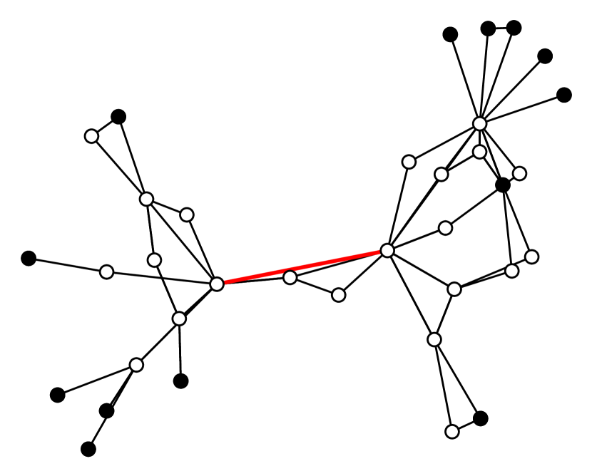
All the curves (gray lines in Fig. 13), not only of these somewhat arbitrarily chosen subsets, show drops of various magnitude at a variety of distances to the added line. We conclude that all of them are triggered by the extent and nature of the connectivity of the graph at that particular distance. Note that in this study, the results are averaged over all lines of a particular distance, regardless of direction. As the structural properties of the grid can be quite different in different regions of the grid, a clear tendency (for example strong drops) can only be observed for some examples in which the properties change at about the same distance in all directions. It can however be expected that the same mechanisms lead to the deviations from the power law in all the curves, at all distances. A future study should look at this more closely, following the response behavior through an irregular graph for each path in each direction separately.
We became aware of a recent work that examined the influence of the addition of a single on the linear stability of an existing synchronous state Coletta2016 . For a simple ring topology, a classification scheme for the increase or decrease of linear stability has been found. It is also demonstrated that similar effects can be observed in real power grid topologies, considering a model for the British power grid. It would be interesting to further investigate the relation between the two studies.
To conclude, we have shown numerically that local grid modifications – here in form of the addition of a single transmission line – cause a long-range response in AC electricity grids. We have identified a power law decay over a wide range of distances to the perturbation, and quantitavely analyzed the value of the power exponent for the case of a simple square grid topology. This finding can also be relevant for other types of perturbations, for example fluctuations in the power production of small, decentrally placed generators (photovoltaics, wind power), as small changes in the generated power or small phase perturbations Kettemann2015 can have an impact on the stable operation of a large part of the grid.
The power exponent is found to increase with system size and saturate at a value of in the medium distance regime. Further, the power exponent decreases when approaching the critical power transmission capacity of the system beyond which no stable state can be found anymore, and that is distinct for a given topology and load distribution. It would be interesting to investigate more closely how the power exponent approaches the maximal power transmission capacity in a future study.
In real grids, like the considered model for the German transmission grid, the response decays roughly with a power law exponent of 2 as well, but varies strongly depending on the position of the added line within the grid and the grid structure at each particular distance. We find indications that the decay rate depends on the connectivity properties of the grid in a particular distance to the topological perturbation. This finding underlines the importance of this and following works on this problem, as certain local grid structures seem to increase the decay rate of a perturbation, while others lead to a strong decrease.
We conclude that grid regions that are only weakly connected with each other (islanding) can effectively prevent the spreading of perturbations into other regions of the grid, but a weak connectivity between them comes with the expense of redundancy and hence reliability. In the extreme case, where two regions are connected by only one common node, no power flow changes can move from one region to the other due to the lack of alternative routes, but its failure is more dramatic, as the stability of the grid then depends solely on the ability of each “island” to operate independently, and the n-1 criterion is not fulfilled.
This study could be extended to other topologies like random graphs with controllable structural properties Schultz2014 , but also to real world topologies including realistic line parameters and load distributions. Furthermore, the analysis could be extended to the case where the grid is not purely inductive (with varying nodal voltages), using the complete AC power flow equations with the reactive power . Ultimately, this approach could lead to quantitative predictions if a particular grid extension measure improves or diminishes the overall stability and controllability of power transmission grids.
Acknowledgements.
The numerical calculations have been performed using computational resources of the Computational Laboratories for Analysis, Modeling and Visualization (CLAMV), Jacobs University Bremen, Germany. We gratefully acknowledge support of BMBF, CoNDyNet, FK. 03SF0472A.References
- (1) D. Witthaut and M. Timme, The European Physical Journal B 86, 377 (2013).
- (2) D. Labavić, R. Suciu, H. Meyer-Ortmanns, and S. Kettemann, Eur. Phys. J. Spec. Top. 223, 2517 (2014).
- (3) Versorgungsqualität – SAIDI-Werte 2006-2014, Bundesnetzagentur (2015).
- (4) K. Heuck, K.-D. Dettmann, and D. Schulz, Elektrische Energieversorgung, 9th ed. (Springer Fachmedien Wies- baden, Wiesbaden, 2013).
- (5) The star symbol (*) denotes the complex conjugate.
- (6) S. Kettemann, Phys. Rev. Lett., to be published, arxiv:1504.05525v2 (2015).
- (7) G. Filatrella, A. H. Nielsen, and N. F. Pedersen, Eur. Phys. J. B 61, 485 (2008).
- (8) T. Nishikawa, A. E. Motter, New J. Phys. 17, 015012 (2015).
- (9) We use the Python function scipy.optimize.fsolve Jones2001 ; Oliphant2007 , which is a wrapper around the functions hybrd and hybrj of the Fortran package MINPACK minpack .
- (10) E. Jones, T. Oliphant, P. Peterson, and others, SciPy: Open source scientific tools for Python (2001).
- (11) Travis E. Oliphant. Python for Scientific Computing, Computing in Science & Engineering 9, 10-20 (2007), DOI:10.1109/MCSE.2007.58
- (12) J. J. Moré, B. S. Garbow, and K. E. Hillstrom, User Guide for MINPACK-1, Tech. Rep. ANL-80-74 (Argonne National Laboratory, Argonne, IL, USA, 1980).
- (13) Note that there may exist multiple stable solutions that differ from each other by loop currents Delabays2016 . Our method is not able to distinguish between different stable solutions. As a starting vector for the phase solver, we always use zero phase angles. As the topological perturbation can be considered small, the solver will most likely return a stable state in the vicinity of the old one.
- (14) R. Delabays, T. Coletta, and P. Jacquod, J. of Math. Phys. 57, 032701 (2016).
- (15) Similar to the “antiferromagnetic groundstate” known from solid state theory.
- (16) For , the periodic arrangement of generators and consumers remains as the only possible realization, in which every generator is surrounded by four consumers and vise versa.
-
(17)
To assess the quality of the fits, we compute the
goodness of fit probability (GOF) Bevington2002
where(12)
is the chi-squared distribution Bevington2002 and is the number of degrees of freedom (DOF). is the number of data points and the number of fit parameters in the fit model.(13) - (18) P. Bevington and D. K. Robinson, Data Reduction and Error Analysis for the Physical Sciences, 3rd ed. (McGraw-Hill Education, Boston, 2002), p. 336.
- (19) The error bars correspond to a confidence level of if they are calculated as , where is the mean of the data and the standard error of the mean.
- (20) The data error in our fits is solely given by the standard error of the mean, so an underestimation of the uncertainty in the raw data cannot be the cause of the bad GOF probabilities gof .
- (21) SciGRID v0.1, NEXT ENERGY – EWE Research Centre for Energy Technology, http://www.scigrid.de/.
- (22) T. Coletta, and P. Jacquod, Phys. Rev. E 93, 032222 (2016).
- (23) P. Schultz, J. Heitzig, and J. Kurths, Eur. Phys. J. Special Topics 223, 2593 (2014).
| 10 | 3 | 1 | |||||
| 20 | 3 | 1 | |||||
| 30 | 3 | 1 | |||||
| 40 | 3 | 1 | |||||
| 50 | 3 | 1 | |||||
| 60 | 3 | 1 | |||||
| 70 | 3 | 1 | |||||
| 80 | 3 | 1 | |||||
| 10 | 3 | 1 | |||||
| 20 | 3 | 1 | |||||
| 30 | 3 | 1 | |||||
| 40 | 3 | 1 | |||||
| 50 | 3 | 1 | |||||
| 60 | 3 | 1 | |||||
| 70 | 3 | 1 | |||||
| 80 | 3 | 1 | |||||
| 10 | 3 | 1 | |||||
| 20 | 3 | 1 | |||||
| 30 | 3 | 1 | |||||
| 40 | 3 | 1 | |||||
| 50 | 3 | 1 | |||||
| 60 | 3 | 1 | |||||
| 70 | 3 | 1 | |||||
| 80 | 3 | 1 | |||||
| 10 | 3 | 1 | |||||
| 20 | 3 | 1 | |||||
| 30 | 3 | 1 | |||||
| 40 | 3 | 1 | |||||
| 50 | 3 | 1 | |||||
| 60 | 3 | 1 | |||||
| 70 | 3 | 1 | |||||
| 80 | 3 | 1 | |||||
| 10 | 3 | 1 | |||||
| 20 | 3 | 1 | |||||
| 30 | 3 | 1 | |||||
| 40 | 3 | 1 | |||||
| 50 | 3 | 1 | |||||
| 60 | 3 | 1 | |||||
| 70 | 3 | 1 | |||||
| 80 | 3 | 1 |
| 20 | 4 | 2 | |||||
| 30 | 8 | 6 | |||||
| 40 | 12 | 10 | |||||
| 50 | 16 | 14 | |||||
| 60 | 20 | 18 | |||||
| 70 | 24 | 22 | |||||
| 80 | 28 | 26 | |||||
| 20 | 4 | 2 | |||||
| 30 | 8 | 6 | |||||
| 40 | 12 | 10 | |||||
| 50 | 16 | 14 | |||||
| 60 | 20 | 18 | |||||
| 70 | 24 | 22 | |||||
| 80 | 28 | 26 | |||||
| 20 | 4 | 2 | |||||
| 30 | 8 | 6 | |||||
| 40 | 12 | 10 | |||||
| 50 | 16 | 14 | |||||
| 60 | 20 | 18 | |||||
| 70 | 24 | 22 | |||||
| 80 | 28 | 26 | |||||
| 20 | 4 | 2 | |||||
| 30 | 8 | 6 | |||||
| 40 | 12 | 10 | |||||
| 50 | 16 | 14 | |||||
| 60 | 20 | 18 | |||||
| 70 | 24 | 22 | |||||
| 80 | 28 | 26 | |||||
| 20 | 4 | 2 | |||||
| 30 | 8 | 6 | |||||
| 40 | 12 | 10 | |||||
| 50 | 16 | 14 | |||||
| 60 | 20 | 18 | |||||
| 70 | 24 | 22 | |||||
| 80 | 28 | 26 |
| 20 | 6 | 4 | |||||
| 30 | 9 | 7 | |||||
| 40 | 12 | 10 | |||||
| 50 | 15 | 13 | |||||
| 60 | 18 | 16 | |||||
| 70 | 21 | 19 | |||||
| 80 | 24 | 22 | |||||
| 20 | 6 | 4 | |||||
| 30 | 9 | 7 | |||||
| 40 | 12 | 10 | |||||
| 50 | 15 | 13 | |||||
| 60 | 18 | 16 | |||||
| 70 | 21 | 19 | |||||
| 80 | 24 | 22 | |||||
| 20 | 6 | 4 | |||||
| 30 | 9 | 7 | |||||
| 40 | 12 | 10 | |||||
| 50 | 15 | 13 | |||||
| 60 | 18 | 16 | |||||
| 70 | 21 | 19 | |||||
| 80 | 24 | 22 | |||||
| 20 | 6 | 4 | |||||
| 30 | 9 | 7 | |||||
| 40 | 12 | 10 | |||||
| 50 | 15 | 13 | |||||
| 60 | 18 | 16 | |||||
| 70 | 21 | 19 | |||||
| 80 | 24 | 22 | |||||
| 20 | 6 | 4 | |||||
| 30 | 9 | 7 | |||||
| 40 | 12 | 10 | |||||
| 50 | 15 | 13 | |||||
| 60 | 18 | 16 | |||||
| 70 | 21 | 19 | |||||
| 80 | 24 | 22 |