Constraining SN feedback: a tug of war between reionization and the Milky Way satellites

Abstract

Theoretical models of galaxy formation based on the cold dark matter cosmogony typically require strong feedback from supernova (SN) explosions in order to reproduce the Milky Way satellite galaxy luminosity function and the faint end of the field galaxy luminosity function. However, too strong a SN feedback also leads to the universe reionizing too late, and the metallicities of Milky Way satellites being too low. The combination of these four observations therefore places tight constraints on SN feedback. We investigate these constraints using the semi-analytical galaxy formation model galform. We find that these observations favour a SN feedback model in which the feedback strength evolves with redshift. We find that, for our best fit model, half of the ionizing photons are emitted by galaxies with rest-frame far-UV absolute magnitudes $M_{\rm AB}(1500{\rm\AA})<-17.5$, which implies that already observed galaxy populations contribute about half of the photons responsible for reionization. The $z=0$ descendants of these galaxies are mainly galaxies with stellar mass $M_{*}>10^{10}\,{\rm M}_{\odot}$ and preferentially inhabit halos with mass $M_{\rm halo}>10^{13}\,{\rm M}_{\odot}$.

1 introduction

Supernova feedback (SN feedback hereafter) is a very important physical process for regulating the star formation in galaxies (Larson, 1974; Dekel & Silk, 1986; White & Frenk, 1991). Despite its importance, SN feedback is not well understood. Perhaps the best way to improve our understanding of this process is by investigating its physical properties using hydrodynamical simulations. This, however, is very difficult to achieve with current computational power: cosmological hydrodynamical simulations (e.g. Davé et al., 2013; Vogelsberger et al., 2014; Schaye et al., 2015) can provide large galaxy samples and can follow galaxy evolution spanning the history of the Universe, but do not have high enough resolution to follow individual star forming regions, which is needed to understand the details of SN feedback; conversely high resolution hydrodynamical simulations (e.g. Bate, 2012; Hopkins et al., 2012) can resolve many more details of individual star forming regions, but do not provide a large sample and cannot follow a long period of evolution. Because of these limitations, it is worth trying to improve our understanding of SN feedback in alternative ways. One promising approach is to extract constraints on SN feedback from theoretical models of galaxy formation combined with observational constraints.

Among all relevant observations, a combination of four observables may be particularly effective because they constrain the strength of feedback in opposite directions. These are the abundance of faint galaxies, including both the faint ends of the $z=0$ field galaxy luminosity function (hereafter field LF) and the Milky Way satellite luminosity function (hereafter MW sat LF), the Milky Way satellite stellar metallicity vs. stellar mass correlation (hereafter MW sat $Z_{*}\--M_{*}$ correlation) and the redshift, $z_{\rm re,half}$, at which the Universe was 50% reionized. The observed abundance of faint galaxies is very low compared to the abundance of low mass dark matter halos in the standard cold dark matter (CDM) model of cosmogony (e.g. Benson et al., 2003; Moore et al., 1999; Klypin et al., 1999), which cannot be reproduced by very weak SN feedback, and this puts a lower limit on the SN feedback strength. On the other hand, $z_{\rm re,half}$ and the MW sat $Z_{*}\--M_{*}$ correlation put upper limits on the SN feedback strength, because too strong a SN feedback would cause too strong a metal loss and a suppression of star formation in galaxies, thus leading to too low $Z_{*}$ at a given $M_{*}$, and too low $z_{\rm re,half}$. Also note that this combination of observations constrains SN feedback over a wide range of galaxy types and redshifts: the field LF mainly provides constraints on SN feedback in larger galaxies, with circular velocity $V_{\rm c}\gtrsim 80\,{\rm km}\,{\rm s}^{-1}$, while $z_{\rm re,half}$ mainly constrains SN feedback at $z\gtrsim 8$, and the Milky Way satellite observations (MW sat LF and MW sat $Z_{*}\--M_{*}$ correlation) provide constraints on the SN feedback in very small galaxies, i.e. $V_{\rm c}\lesssim 40\,{\rm km}\,{\rm s}^{-1}$, and probably over a wide redshift range, from very high redshift to $z\sim 1$. (This is because recent observations (e.g. de Boer et al., 2012; Vargas et al., 2013) indicate that the Milky Way satellites have diverse star formation histories, with some of them forming all of their stars very early, and others having very extended star formation histories.)

In this work, we investigate the constraints placed by this combination of observations on SN feedback using the semi-analytical galaxy formation model galform (Cole et al., 2000; Baugh et al., 2005; Bower et al., 2006; Lacey et al., 2015). A semi-analytical galaxy formation model is ideal for this aim, because with it one can generate large samples of galaxies with high mass resolution, which is important for simulating both Milky Way satellites and star formation at high redshift, and it is also computationally feasible to explore various physical models and parameterizations.

This paper is organized as follows. Section 2 describes the starting point of this work, the Lacey et al. (2015) (hereafter Lacey16) galform model, as well as extensions of this model and details of the simulation runs. Section 3 presents the results from the Lacey16 and modified models. Section 4 discusses the physical motivation for some of the modifications, and also which galaxies drive cosmic reionization and what their $z=0$ descendants are. Finally a summary and conclusions are given in Section 5.

2 methods

2.1 Starting point: Lacey16 model

The basic model used in this work is the Lacey16 (Lacey et al., 2015) model, a recent version of galform. This model, and the variants of it that we consider in this paper, all assume a flat $\Lambda$CDM universe with cosmological parameters based on the WMAP-7 data (Komatsu et al., 2011): $\Omega_{\rm m0}=0.272$, $\Omega_{\rm v0}=0.728$, $\Omega_{\rm b0}=0.0455$ and $H_{0}=70.4~{}\,{\rm km}\,{\rm s}^{-1}{\rm Mpc}^{-1}$, and an initial power spectrum with slope $n_{\rm s}=0.967$ and normalization $\sigma_{8}=0.810$. The Lacey16 model implements sophisticated modeling of disk star formation, improved treatments of dynamical friction on satellite galaxies and of starbursts triggered by disk instabilities and an improved stellar population synthesis model; it reproduces a wide range of observations, including field galaxy luminosity functions from $z=0$ to $z=3$, galaxy morphological types at $z=0$, and the number counts and redshift distribution of submillimetre galaxies. An important feature of this model is that it assumes a top-heavy IMF for stars formed in starbursts, which is required to fit the submillimeter data, while stars formed by quiescent star formation in disks have a Solar neighbourhood IMF. Stellar luminosities of galaxies at different wavelengths, and the production of heavy elements by supernovae, are predicted self-consistently, allowing for the varying IMF.

SN feedback is modeled in this and earlier versions of galform as follows. SN feedback ejects gas out of galaxies, and thus reduces the amount of cold gas in galaxies, regulating the star formation. The gas ejection rate is formulated as:

$$\dot{M}_{\rm eject}=\beta\psi,$$ (1)

where $\dot{M}_{\rm eject}$ is the mass ejection rate, $\psi$ is the star formation rate and the mass-loading factor, $\beta$, encodes the details of SN feedback models. In the approximation of instantaneous recycling that we use here, in which we neglect the time delay between the birth and death of a star, the supernova rate, and hence also the supernova energy injection rate, are proportional to the instantaneous star formation rate $\psi$.

In the Lacey16 model, $\beta$ is set to be a single power law in galaxy circular velocity, $V_{\rm c}$, specifically,

$$\beta=\left(\frac{V_{\rm c}}{V_{\rm SN}}\right)^{-\gamma_{\rm SN}},$$ (2)

where $V_{\rm SN}$ and $\gamma_{\rm SN}$ are two free parameters. In the Lacey16 model, $V_{\rm SN}=320\,{\rm km}\,{\rm s}^{-1}$ and $\gamma_{\rm SN}=3.2$. $\beta$ as a function of $V_{\rm c}$ for the Lacey16 model is illustrated in the left panel of Fig. 1.

As shown in Figs. 3 and 5, the above single power-law SN feedback model is disfavored by the combination of the four observational constraints mentioned in §1. We therefore investigate some modified SN feedback models and test them against the same set of observations. These modified models are described next.

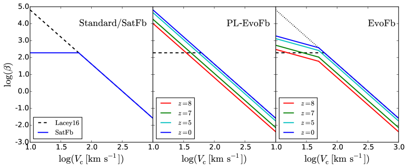
Figure 1: Mass-loading factor, $\beta$, as a function of circular velocity, $V_{\rm c}$, and redshift, $z$, for the different supernova feedback models used in this work. Left panel: The dashed black line shows $\beta$ in the Lacey16 model, while the solid blue line shows $\beta$ for the SatFb model. Middle panel: $\beta$ for the PL-EvoFb model. Different colours indicate different redshifts (from top to bottom, redshift increases from $0$ to $8$). This model is identical to the Lacey16 model for $z\leq 4$ (solid blue line). The SatFb model is also plotted as a dashed line for reference. Right panel: $\beta$ for the EvoFb model. Different colours indicate different redshifts (from top to bottom, redshift increases from $0$ to $8$). $\beta$ for the Lacey16 and SatFb models are also plotted for reference, and are shown by the black dotted and dashed lines respectively.

2.2 Modified SN feedback models

In the modified SN feedback models we assume a broken power law for $\beta$, with a change in slope below a circular velocity, $V_{\rm thresh}$:

$$\beta=\left\{\begin{array}[]{cc}(V_{\rm c}/V_{\rm SN})^{-\gamma_{\rm SN}}&V_{\rm c}\geq V_{\rm thresh}\\ (V_{\rm c}/V^{\prime}_{\rm SN})^{-\gamma^{\prime}_{\rm SN}}&V_{\rm c}<V_{\rm thresh}\end{array}\right..$$ (3)

Here $V_{\rm SN}$, $\gamma_{\rm SN}$, $V_{\rm thresh}$ and $\gamma^{\prime}_{\rm SN}$ are free parameters, while $V^{\prime}_{\rm SN}$ is fixed by the condition that the two power laws should join at $V_{\rm c}=V_{\rm thresh}$.

2.2.1 Saturated feedback model

In this class of models we set $\gamma^{\prime}_{\rm SN}<\gamma_{\rm SN}$, so that the mass-loading factor, $\beta$, for $V_{\rm c}<V_{\rm thresh}$ is lower than in the single power-law model. Note that we require $\gamma^{\prime}_{\rm SN}\geq 0$, because a negative $\gamma^{\prime}_{\rm SN}$ would predict an anti-correlation between galaxy stellar metallicity and stellar mass, in contradiction with observations of the MW satellites.

A similar feedback model, with $\gamma^{\prime}_{\rm SN}=0$, was previously used by Font et al. (2011), which showed that it improved the agreement of galform model predictions with Milky Way observations. However, in the present work, the observational constraints are more stringent than in Font et al. (2011), because here not only are Milky Way observations considered, but also the field LF and the reionization redshift.

In this work, we investigate a specific saturated feedback model, with $V_{\rm thresh}=62\,{\rm km}\,{\rm s}^{-1}$ and $\gamma^{\prime}_{\rm SN}=0$, which implies that $\beta$ is a constant for galaxies with $V_{\rm c}<62\,{\rm km}\,{\rm s}^{-1}$ but reduces to the standard Lacey16 form for $V_{\rm c}>V_{\rm thresh}$. We call this specific saturated feedback model SatFb. The mass-loading factor for this model is also illustrated in the left panel of Fig. 1.

2.2.2 Evolving feedback model

This class of model has weaker SN feedback strength at high redshift. Here we investigate two specific models. For the first one, called PL-EvoFb, the feedback strength is a single power law in $V_{\rm c}$ at any redshift, but the normalization changes with redshift, being identical to the Lacey16 model for $z\leq 4$, but lower at high redshifts, Specifically, this model has $\gamma^{\prime}_{\rm SN}=\gamma_{\rm SN}=3.2$ (as in Lacey16) and

$$V_{\rm SN}\ [{\rm km}\,{\rm s}^{-1}]=\left\{\begin{array}[]{cc}180&z>8\\ -35z+460&4\leq z\leq 8\\ 320&z<4\end{array}\right..$$ (4)

The general behaviour of this model is motivated by the results of Lagos et al. (2013), who predicted mass-loading factors from a detailed model of SN-driven superbubbles expanding in the ISM. (The Lagos et al. model was however incomplete, in that it considered only gas ejection out of the galaxy disk, but not out of the halo.) The mass loading factor, $\beta$, for this model is illustrated in the middle panel of Fig. 1.

The second model that we try, called EvoFb, has a normalization that evolves with redshift as in the PL-EvoFb model, but also has a shallower $V_{\rm c}$-dependence at low $V_{\rm c}$. Specifically, this model has $\gamma_{\rm SN}=3.2$ (as in Lacey16), $\gamma^{\prime}_{\rm SN}=1.0$, $V_{\rm thresh}=50\,{\rm km}\,{\rm s}^{-1}$ and $V_{\rm SN}(z)$ as given in Eq (4). For $V_{\rm c}>50\,{\rm km}\,{\rm s}^{-1}$, this model is identical to the PL-EvoFb model, but it has weaker feedback for $V_{\rm c}\leq 50\,{\rm km}\,{\rm s}^{-1}$. The saturation in $\beta$ at low $V_{\rm c}$ is therefore weaker than in the SatFb model. The mass loading factor for this model is illustrated in the right panel of Fig. 1.

The physical motivation for introducing the redshift evolution in the SN feedback will be discussed further in §4.

2.3 The redshift of reionization and photoionization feedback

We estimate the redshift of reionization predicted by a galform model by calculating the ratio, ${\cal R}(z)$, of the number density of ionizing photons produced up to that redshift to the number density of hydrogen nuclei:

$${\cal R}(z)=\frac{\int_{z}^{\infty}\epsilon(z^{\prime})dz^{\prime}}{n_{\rm H}},$$ (5)

where $\epsilon(z^{\prime})$ is the number of hydrogen-ionizing photons produced per unit comoving volume per unit redshift at redshift $z^{\prime}$, and $n_{\rm H}$ is the comoving number density of hydrogen nuclei.

The Universe is assumed to be fully ionized at a redshift, $z_{\rm re,full}$, for which,

$${\cal R}(z_{\rm re,full})=\frac{1+N_{\rm rec}}{f_{\rm esc}},$$ (6)

where $N_{\rm rec}$ is the mean number of recombinations per hydrogen atom up to reionization, and $f_{\rm esc}$ is the fraction of ionizing photons that can escape from the galaxies producing them into the IGM. In this paper we adopt $N_{\rm rec}=0.25$ and $f_{\rm esc}=0.2$, and thus the threshold for reionization is ${\cal R}(z_{\rm re,full})=6.25$. Below we justify these choices.

Our estimation of the reionization redshift using ${\cal R}(z)$ (Eqs (5) and (6)) appears to be different from another commonly used estimator based on $Q_{\rm HII}$, defined as the volume fraction of ionized hydrogen, with reionization being complete when $Q_{\rm HII}=1$, but in fact they are essentially equivalent. The evolution equation for $Q_{\rm HII}$ is given in Madau et al. (1999) as $\dot{Q}_{\rm HII}=\dot{n}_{\rm ion}/n_{\rm H}-Q_{\rm HII}/\bar{t}_{\rm rec}$, where $n_{\rm ion}$ is the comoving number density of ionizing photons escaping into IGM and $\bar{t}_{\rm rec}$ is the mean recombination time scale. Integrating both sides of this equation from $t=0$ to the time $t=t_{\rm re,full}$ when reionization completes, one obtains

$$Q_{\rm HII}(t_{\rm re,full})$$ (7)

$$= \frac{\int_{0}^{t_{\rm re,full}}\dot{n}_{\rm ion}\,dt}{n_{\rm H}}-\frac{\int_{0}^{t_{\rm re,full}}[n_{\rm H}Q_{\rm HII}/\bar{t}_{\rm rec}]\,dt}{n_{\rm H}}$$

$$= \frac{f_{\rm esc}\int_{z_{\rm re,full}}^{\infty}\epsilon(z^{\prime})dz^{\prime}}{n_{\rm H}}-\frac{n_{\rm rec,tot}}{n_{\rm H}}$$

where $n_{\rm rec,tot}$ is the mean number of recombinations per comoving volume up to $z_{\rm re,full}$. Setting $Q_{\rm HII}(t_{\rm re,full})=1$ and defining $N_{\rm rec}={n_{\rm rec,tot}}/{n_{\rm H}}$, one then obtains Eq (6) for $z_{\rm re,full}$.

With the expression for $\bar{t}_{\rm rec}$ given by Madau & Haardt (2015) (their Eqn 4), $N_{\rm rec}$ can be expressed as

$$N_{\rm rec}=\int_{0}^{t_{\rm re,full}}[Q_{\rm HII}(1+\chi)\alpha_{\rm B}(1+z)^{3}C_{\rm RR}]dt$$ (8)

where $\chi=0.083$, $\alpha_{\rm B}$ is the case-B recombination rate coefficient and $C_{\rm RR}$ the clumping factor. Using the clumping factor in Shull et al. (2012) and solving the equation for $Q_{\rm HII}$, Eqn (8) gives $N_{\rm rec}$ in the range $0.13-0.34$ for our four different SN feedback models and an IGM temperature, $T=1-2\times 10^{4}\,{\rm K}$. Our choice of $N_{\rm rec}=0.25$ lies within this range; note that Eqn (6) is not very sensitive to $N_{\rm rec}$ when its value is much smaller than $1$. Our choice for $N_{\rm rec}$ is lower than the values assumed in some previous works (e.g. Raičević et al., 2011) because recent simulations give lower clumping factors (see Finlator et al. 2012 and references therein).

The calculation of $\epsilon(z^{\prime})$ requires a knowledge of the ionizing sources. The traditional assumption has been that these sources are mainly star-forming galaxies, but recently there have been some works (e.g. Fontanot et al., 2012; Madau & Haardt, 2015; Giallongo et al., 2015) suggesting that AGN could be important contributors to reionization of hydrogen in the IGM. Although AGN might be important for reionization, these current works rely on extrapolatiing the AGN luminosity function faintwards of the observed luminosity limit, and also extrapolating the observations at $z\leq 6$ to $z\sim 10$, in order to obtain a significant contribution to reionization from AGN. These extrapolations are uncertain, therefore in this work we ignore any AGN contribution and assume that the ionizing photon budget for reionization is dominated by galaxies. We discuss how the AGN contribution affects our conclusion in more detail in §4.4.

The value of the escape fraction, $f_{\rm esc}$, is also uncertain. Numerical simulations including gas dynamics and radiative transfer have given conflicting results: Kimm & Cen (2014) estimated $f_{\rm esc}\sim 0.1$, with $f_{\rm esc}\sim 0.2$ for starbursts, while Paardekooper et al. (2015) found much lower values. These differences between simulations may result from differences in the modelling of the ISM or in how well it is resolved, both of which are challenging problems. Observationally, it is impossible to measure $f_{\rm esc}$ directly for galaxies at the reionization epoch, because escaping ionizing photons would, in any case, be absorbed by the partially neutral IGM. Thus, one has to rely on observations of lower redshift galaxies for clues to its value.

Observations of Lyman-break galaxies at $z=3-4$ suggest a relatively low value, $f_{\rm esc}\sim 0.05$ (Vanzella et al., 2010), while observations of local compact starburst galaxies show indirect evidence for higher $f_{\rm esc}$ (e.g. Alexandroff et al., 2015); Borthakur et al. (2014) estimated $f_{\rm esc}=0.21$ for one local example. It is therefore important to determine what class of currently observed galaxies are the best analogues of galaxies at the reionization epoch. In our simulations, galaxies at high redshift tend to be compact and, in addition, the galaxies dominating the ionizing photon budget are starbursts (see Fig. 8), so, as argued by Sharma et al. (2016), they may well have similar escape fractions to local compact starburst galaxies. Sharma et al. (2016) provide further arguments that support our choice of $f_{\rm esc}=0.2$. We discuss how the uncertainties in $f_{\rm esc}$ affect our conclusions in more detail in §4.4.

Note that, as advocated by Sharma et al. (2016) we only assume $f_{\rm esc}=0.2$ for $z\geq 5$; for lower redshifts, $f_{\rm esc}$ may drop to low values, consistent with recent studies which argue that $f_{\rm esc}$ evolves with redshift and increases sharply for $z>4$ (e.g. Haardt & Madau, 2012; Kuhlen & Faucher-Giguère, 2012) .

Observations of the CMB directly constrain the electron scattering optical depth to recombination, which is then converted to a reionization redshift by assuming a simple model for the redshift dependence of the ionized fraction. Papers by the WMAP and Planck collaborations (e.g. Planck Collaboration et al., 2014) typically express the reionization epoch in terms of the redshift, $z_{\rm re,half}$, at which the IGM is 50% ionized, by using the simple model for non-instantaneous reionization described in Appendix B of Lewis (2008). For comparing with such observational estimates, we therefore calculate $z_{\rm re,half}$ from galform by assuming ${\cal R}(z_{\rm re,half})=\frac{1}{2}{\cal R}(z_{\rm re,full})$. For the abovementioned choices of $N_{\rm rec}$ and $f_{\rm esc}$, this is equivalent to ${\cal R}(z_{\rm re,half})=3.125$.

Reionization may suppress galaxy formation in small halos, an effect called photoionization feedback (Couchman & Rees, 1986; Efstathiou, 1992; Thoul & Weinberg, 1996). In this work, the photoionization feedback is modeled using a simple approximation (Benson et al., 2003), in which dark matter halos with circular velocity at the virial radius $V_{\rm vir}<V_{\rm crit}$ have no gas accretion or gas cooling for $z<z_{\rm crit}$. As shown by Benson et al. (2002) and Font et al. (2011), this method provides a good approximation to a more complex, self-consistent photoionization feedback model. Here, $V_{\rm crit}$ and $z_{\rm crit}$ are two free parameters. In this paper, unless otherwise specified, we adopt $z_{\rm crit}=z_{\rm re,full}$ and $V_{\rm crit}=30\,{\rm km}\,{\rm s}^{-1}$. This value of $V_{\rm crit}$ is consistent with the hydrodynamical simulation results of Okamoto et al. (2008). Note that this method does not necessarily imply that star formation in galaxies in halos with $V_{\rm vir}<V_{\rm crit}$ is turned off immediately after $z=z_{\rm re,full}$. The star formation in these galaxies can continue as long as the galaxy cold gas reservoir is not empty.

2.4 Simulation runs

Studying reionization requires resolving galaxy formation in low mass halos ($M_{\rm vir}\sim 10^{8}\--10^{10}\,{\rm M}_{\odot}$) at high redshifts ($z\sim 7\--15$), and thus very high mass resolution for the dark matter halo merger trees. The easiest way to achieve this high resolution is to use Monte Carlo (MC) merger trees.

Studying the properties of the Milky Way satellites also requires very high mass resolution because the host halos of these small satellites are small. This too is easily achieved using MC merger trees. Furthermore, because building MC merger trees is computationally inexpensive, it is possible to build a large statistical sample of Milky Way-like halos to study their satellites.

In this work we generate MC merger trees using the method of Parkinson et al. (2008). To study reionization, we ran simulations starting at $z_{\rm start}=20$ down to different final redshifts, $z_{\rm end}$, to derive $\epsilon(z)$ defined in Eq (5) at $z=5\--15$ and the $z=0$ field LF. We scale the minimum progenitor mass in the merger trees as $(1+z_{\rm end})^{-3}$, with a minimum resolved mass, $M_{\rm res}=7\times 10^{9}\,{\rm M}_{\odot}$ for $z_{\rm end}=0$. We have tested that these choices are sufficient to derive converged results. For the Milky Way satellite study, the present-day host halo mass is chosen to be in the range $5\times 10^{11}\--2\times 10^{12}\,{\rm M}_{\odot}$, which represents the current observational constraints on the halo mass of the Milky Way, and we sample this range with five halo masses evenly spaced in log(mass). For each of these halo masses, galform is run on $100$ MC merger trees, with minimum progenitor mass $M_{\rm res}=1.4\times 10^{6}\,{\rm M}_{\odot}$, which is small enough for modeling the Milky Way satellites, and $z_{\rm start}=20$ and $z_{\rm end}=0$. We do not attempt to select Milky Way-like host galaxies, because we found that the satellite properties correlate better with the host halo mass than with the host galaxy properties.

3 results

In this section, we show how the results from the different models compare with the key observational constraints that we have identified, namely: the field galaxy luminosity functions at $z=0$; the redshift of reionization; the MW satellite galaxy luminosity function; and the stellar metallicity vs stellar mass relation for MW satellites.

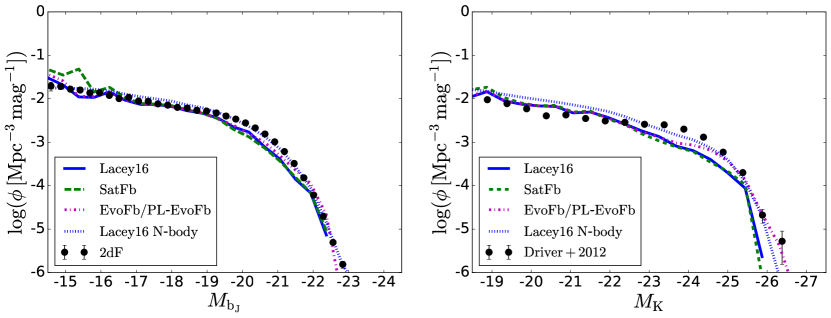
Figure 2: $z=0$ field luminosity functions. The left panel shows the $b_{J}$-band luminosity function and the right panel the $K$-band luminosity function. In both panels the solid, dashed and dashed-dotted lines with different colours show the predictions using Monte Carlo merger trees for different SN feedback models, as indicated in the line key, while the blue dotted lines are for the Lacey16 model run with N-body merger trees. The magenta lines show the results of the EvoFb model, but the results for the PL-EvoFb model are almost identical. The black points with errorbars are observational data, from Norberg et al. (2002) for the $b_{J}$-band and from Driver et al. (2012) for the $K$-band.

3.1 Lacey16 model

We begin by showing the results for the default Lacey16 model, since this then motivates considering models with modified SN feedback. Fig. 2 shows the $b_{J}$- and $K$-band field LFs of different models at $z=0$ (left and right panels respectively). The dotted blue lines show the LFs calculated using N-body merger trees, as used in the original Lacey et al. (2015) paper to calibrate the model parameters. The fit to the observed LFs is seen to be very good. The solid blue lines show the predictions with identical model parameters but instead using MC merger trees, as used in the remainder of this paper. The run with MC merger trees gives slightly lower LFs than the run with the N-body trees around the knee of the LF, but at lower luminosities, the results predicted using MC and N-body merger trees are in good agreement. We remind the reader that we use MC merger trees in the main part of this paper in order to achieve the higher halo mass resolution that we need for the other observational comparisons. Since the differences in the LFs between the two types of merger tree are small, and barely affect the faint end of the field LFs which are the main focus of interest here, we do not consider them important for this paper.

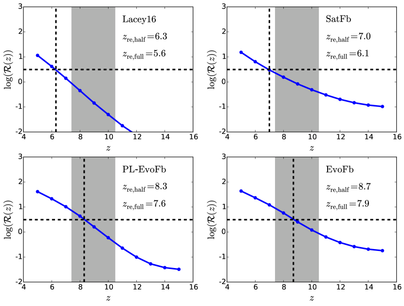
Figure 3: ${\cal R}(z)$, which is the ratio of the total number of ionizing photons produced up to redshift $z$ to the total number of hydrogen nuclei, for different SN feedback models. Each panel shows a different model, as labelled. The blue line shows the predicted ${\cal R}(z)$, while the horizontal dashed line shows the threshold ${\cal R}(z_{\rm re,half})=5$ for 50% reionization, and the vertical dashed line the corresponding redshift $z_{\rm re,half}$. The grey shaded region shows the observational constraint on $z_{\rm re,half}$ from Planck, namely $z_{\rm re}=8.8_{-1.4}^{+1.7}$ ($68\%$ confidence region, Planck Collaboration et al., 2015). The predicted value of the redshift $z_{\rm re,full}$ for 100% reionization is also given in each panel.

Fig. 3 shows the predicted ${\cal R}(z)$ (defined in Eq 5) for different SN feedback models. In each panel, the horizontal black dashed line indicates the criterion for 50% reionization, i.e. ${\cal R}(z_{\rm re,half})=3.125$, the vertical black dashed line indicates $z_{\rm re,half}$ of the corresponding model, and the corresponding value of $z_{\rm re,half}$ is given in the panel. The gray shaded area in each of these panels indicates the current observational constraint from Planck, namely $z_{\rm re}=8.8_{-1.4}^{+1.7}$ ($68\%$ confidence region, Planck Collaboration et al., 2015). The redshift $z_{\rm re,full}$ for full reionization (given by ${\cal R}(z_{\rm re,full})=6.25$) for each model is also given in the corresponding panel. The results for the Lacey16 model are shown in the upper left panel. With the above mentioned criterion, this model predicts $z_{\rm re,half}=6.3$, which is too low compared to the observational estimate. This indicates that in the Lacey16 model, star formation at high redshift, $z\gtrsim 8$, is suppressed too much. There are two possible reasons for this oversuppression: one is the SN feedback at high redshift is too strong, and the other is that the SN feedback in low-mass galaxies is too strong (since the typical galaxy mass is lower at higher redshift).

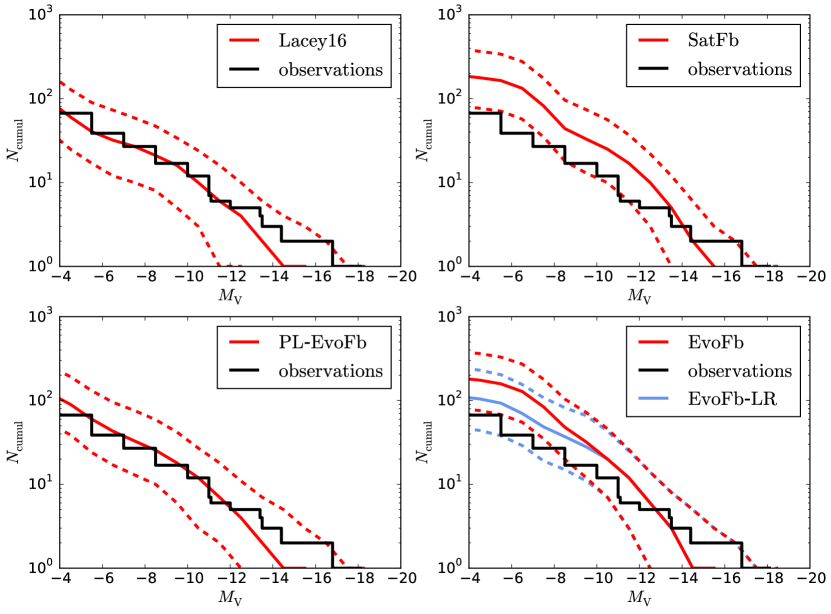
Figure 4: Cumulative luminosity function of satellite galaxies in Milky Way-like host halos at $z=0$. The solid black line in each panel is the observed Milky Way satellite cumulative luminosity function. For $M_{\rm V}<-11$, this shows the direct observational results from McConnachie (2012), while for $M_{\rm V}\geq-11$, it shows the results from Koposov et al. (2008), who applies some corrections for incompleteness in the observations. The other lines in each panel show the model predictions, with the solid red line showing the median for a sample of MW-like halos, and the dashed lines indicating the $5\--95\%$ range. The corresponding model names are given in the line key in each panel.

Fig. 4 shows the cumulative luminosity function of satellite galaxies in Milky Way-like host halos. In each panel, the red solid and dashed lines show the simulation results for the corresponding model. For each model, the simulations were run on 100 separate merger trees for each of 5 host halo masses, evenly spaced in the logarithm of the mass in the range $5\times 10^{11}\--2\times 10^{12}\,{\rm M}_{\odot}$. This simulated sample of MW-like halos contains $500$ halos in total, and the red solid line shows the median satellite LF for this sample, while the red dashed lines indicate the $5\--95\%$ range. The black solid line in each panel shows the observed Milky Way satellite luminosity function. For $M_{\rm V}<-11$, we plot the direct observational measurement from McConnachie (2012). For these brighter magnitudes, current surveys for MW satellites are thought to be complete over the whole sky. For $M_{\rm V}\geq-11$ we plot the observational estimate from Koposov et al. (2008) based on SDSS, which includes corrections for incompleteness due to both partial sky coverage and in detecting satellites in imaging data. The predictions for the Lacey16 model are shown in the upper left panel, and are in very good agreement with the observations.

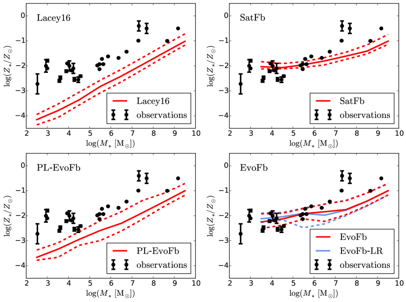
Figure 5: The stellar metallicity ($Z_{*}$) vs stellar mass ($M_{*}$) relation for satellite galaxies in Milky Way-like host halos at $z=0$. The simulated sample for each moel is the same as in Fig. 4. In each panel, the solid line shows the median of the simulated sample, while the dashed lines indicate the $5\--95\%$ range, and the corresponding model name is given in the line key. The black filled circles show the observational results compiled by McConnachie (2012). The observed $[{\rm Fe/H}]$ values in McConnachie (2012) are converted into the total stellar metallicities, $Z_{*}/Z_{\odot}$, in Solar units by assuming the chemical patterns of the observed satellites are Solar. The total metallicities, $Z_{*}$, predicted by the model, which are absolute values, are converted into Solar units assuming $Z_{\odot}=0.0142$ (Asplund et al., 2009).

Fig. 5 shows the $Z_{*}\--M_{*}$ correlation for satellite galaxies in Milky Way-like host halos. The sample is the same as that for Fig. 4. In each panel, the red solid line shows the median of the sample, while the red dashed lines indicate the $5\--95\%$ range. The black filled circles in each panel show observational data. We have converted the observed $[{\rm Fe/H}]$ values into the total stellar metallicities, $Z_{*}/Z_{\odot}$, by assuming that the chemical abundance patterns in the observed satellites are the same as in the Sun. This assumption may lead to an underestimation of the metallicities of low mass satellites, which may not have had enough enrichment by Type Ia supernova to reach the Solar pattern. For these satellites, the observed $Z_{*}$ values shown in the figure are therefore effectively lower limits. The results of the Lacey16 model are again shown in the upper left panel. The $Z_{*}\--M_{*}$ relation predicted by this model is about an order of magnitude below the observations. Because the discrepancy in metallicity is about one order of magnitude, it cannot be caused by inaccuracies in the theoretical stellar yields of metals in this model or by the variation of these yields with stellar metallicity. These yields are obtained by integrating the yields predicted by stellar evolution models over the IMFs assumed for stars formed either quiescently or in starbursts. Assuming that the true metal yields are similar to what is assumed in the model, then for a given stellar mass, the total metals produced are fixed, so the low metallicities seen in the Lacey16 model imply that the loss of metals from satellite galaxies is excessive. Since the metal loss is caused by the outflows induced by SN feedback, this indicates that the SN feedback in these small galaxies is too strong.

In summary, the Lacey16 model motivates two types of modification to the SN feedback. One is suppressing SN feedback in small galaxies, which is the saturated feedback model. The other one is suppressing SN feedback at high redshift, i.e. $z\geq 8$, but keeping strong feedback at $z<4$ in order to reproduce the $z=0$ field LFs. This corresponds to the evolving feedback model. Below, these two kinds of modification will be tested one at a time.

3.2 Saturated feedback model (SatFb)

The dashed green lines in Fig. 2 show the ${\rm b}_{\rm J}$-band and ${\rm K}$-band LFs for the SatFb model. These predictions are still roughly consistent with the observations, but a small excess of galaxies begins to appear at the very faint end of the ${\rm b}_{\rm J}$-band LF ($M_{{\rm b}_{\rm J}}>-17$). Reducing the SN feedback strength further in this model would exacerbate this discrepancy.

The upper right panel of Fig. 3 shows ${\cal R}(z)$ for our SatFb model; the predicted $z_{\rm re,half}$ is $7.0$, outside the 1-$\sigma$ region allowed by the Planck observations. Thus, SN feedback in the SatFb model is much too strong to allow production of enough ionizing photons to reionize the Universe early enough. The upper right panel of Fig. 4 shows the satellite LF of Milky Way-like galaxies in the SatFb model. The relatively weak SN feedback in this model leads to an overprediction of faint ($M_{\rm V}\geq-8$) satellites. Bearing in mind the significant uncertainties in the numbers of faint satellites, this model prediction may be deemed to be roughly acceptable. Furthermore, these very faint Milky Way satellites are very small, and so their abundance could be further supressed by adjusting the strength of photoionization feedback. However, this would not help reduce the excess at the faint end of the field LFs, because these galaxies are larger and thus not strongly affected by photoionization feedback. The upper right panel of Fig. 5 shows the satellite $Z_{*}\--M_{*}$ correlation for Milky Way-like hosts. This model prediction agrees with observations only roughly. The correlation is shallow because most of these satellites have $V_{\rm c}<V_{\rm thresh}=62\,{\rm km}\,{\rm s}^{-1}$, and thus similar values of $\beta$.

If the SN feedback strength in the SatFb model were further reduced, the excess in the satellite LF would shift to brighter luminosities, $M_{\rm V}<-8$, where there are fewer uncertainties in the data and where photoionization feedback is ineffective. The stellar metallicity of satellites of a given stellar mass would become even higher, spoiling the already marginal agreement with observations. Together, these results from the Milky Way satellites suggest that the strength of SN feedback in model SatFb is a lower limit to the acceptable value.

This SatFb model therefore does not provide a solution to the problems identified in the Lacey16 model. Further adjustments within the framework of the saturated feedback model would involve changing the saturated power-law slope $\gamma^{\prime}_{\rm SN}$ and/or the threshold velocity, $V_{\rm thresh}$. In the present SatFb model, as mentioned above, $\gamma^{\prime}_{\rm SN}$ is already at its lower limit, namely $0$, and introducing a positive $\gamma^{\prime}_{\rm SN}$ only leads to a stronger SN feedback in small galaxies than in the current SatFb model, and this would not predict a high enough $z_{\rm re,half}$. Reducing $V_{\rm thresh}$ would also lead to a stronger SN feedback in small galaxies than in the current SatFb model, so would not improve the prediction for $z_{\rm re,half}$ either, while enhancing $V_{\rm thresh}$ would lead to a saturation of the SN feedback in even larger galaxies and a stronger saturation in small galaxies than in the current SatFb model. Since the feedback strength in the SatFb model is already as low as allowed by observations of the field LFs, the MW sat LF and the MW sat $Z_{*}\--M_{*}$ relation, this adjustment would only worsen these discrepancies. Thus, the saturated feedback model is disfavoured by this combination of observational constraints.

3.3 Evolving feedback model

3.3.1 PL-EvoFb model

The magenta lines in Fig. 2 show the ${\rm b}_{\rm J}$-band and ${\rm K}$-band field LFs for the PL-EvoFb model. The results are very close to those in the Lacey16 model, and the observed faint ends are well reproduced. This is because in the PL-EvoFb model, the SN feedback at $z\leq 4$ is the same as in the Lacey16 model. The lower left panel in Fig. 3 shows ${\cal R}(z)$ for this model; the corresponding $z_{\rm re,half}$ is $8.3$, which is in agreement with observations. This shows that the evolving feedback model is more successful at generating early reionization than the saturated feedback model.

The lower left panel of Fig. 4 shows the satellite luminosity function of Milky Way-like host halos in the PL-EvoFb model, which is in very good agreement with the observations. The lower left panel of Fig. 5 shows the $Z_{*}\--M_{*}$ relation for satellite galaxies in Milky Way-like host halos in this model. This model predicts stellar metallicities of satellites with $M_{*}\leq 10^{6}\,{\rm M}_{\odot}$ several times to one order of magnitude lower than observations, with the discrepancy increasing with decreasing stellar mass. Although weakening the SN feedback at high redshifts does improve the result compared to the Lacey16 model, it is still inconsistent with observations. Thus this model is disfavoured by observations of MW satellite metallicities. The discrepancy again suggests that the SN feedback in small galaxies is too strong, but since at the same time this model successfully reproduces the faint ends of the field LFs, it suggests that this problem of too strong feedback is restricted to very small galaxies. This then motivates our next model, in which we preferentially suppress the SN feedback strength in very small galaxies, while retaining the same evolution of feedback strength with redshift as in the PL-EvoFb model.

3.3.2 EvoFb model

The field LFs predicted by the EvoFb model are almost identical to those given by the PL-EvoFb model, so this model likewise successfully reproduces the faint ends of the field LFs. The reason for the similarity between the field LFs predicted by the two models is that the saturation introduced in the EvoFb model is only effective for $V_{\rm c}\leq 50\,{\rm km}\,{\rm s}^{-1}$, and would not significantly affect the galaxies in the observed faint ends of the field LFs, which typically have higher $V_{\rm c}$.

The lower right panel in Fig. 3 shows ${\cal R}(z)$ for the EvoFb model; the corresponding $z_{\rm re,half}$ is $8.7$, which is in agreement with the observations. Compared to the result of the PL-EvoFb model, $z_{\rm re,half}$ only increases slightly, so the saturation in the feedback has only a small effect, and the main factor leading to the agreement with observations is still the redshift evolving behavior of the SN feedback strength.

The lower rigth panel of Fig. 4 shows the satellite luminosity function of Milky Way-like host halos in the EvoFb model. The model predictions are roughly consistent with the observations, although the very faint end ($M_{\rm V}\geq-8$) of the MW sat LF is somewhat too high. However, as mentioned in connection with the SatFB model, the observations of this very faint end have significant uncertainties, so this model is still acceptable. The lower right panel of Fig. 5 shows the $Z_{*}\--M_{*}$ relation for the satellite galaxies in Milky Way-like host halos in the EvoFb model. The model predictions are now roughly consistent with the observations. This improvement is achieved by adopting both an evolving SN feedback strength and a saturation of the feedback in galaxies with $V_{\rm c}\leq 50\,{\rm km}\,{\rm s}^{-1}$.

Because the predictions for Milky Way satellites are sensitive to the photoionization feedback, it is possible to further improve the agreement with observations for these galaxies by adjusting the photoionization feedback. One possible adjustment is to adopt the so-called local reionization model (see Font et al. (2011) and references therein), in which higher density regions reionize earlier, so that $z_{\rm re,full}$ for the Local Group region is earlier than the global average $z_{\rm re,full}$ constrained by the Planck data. Earlier reionization means earlier photoionization feedback, so that for the Milky Way satellites one has $z_{\rm crit}>z_{\rm re,full}$. Font et al. (2011) adopted a detailed model to study this local reionization effect, and suggested that using $z_{\rm crit}=10$ gives a good approximation to the results of the more detailed model. Here we also adopt $z_{\rm crit}=10$, and we label the model with evolving SN feedback and $z_{\rm crit}=10$ as EvoFb-LR.

We tested that the predictions for global properties like $z_{\rm re,full}$, $z_{\rm re,half}$ and the field LFs are not very sensitive to the value of $z_{\rm crit}$. It is therefore justified to ignore the variation of $z_{\rm crit}$ with local density when calculating these global properties, and adopt a single $z_{\rm crit}=z_{\rm re,full}$ when predicting these. This also means that introducing such a local reionization model does not allow one to bring the standard Lacey16 or SatFb models into agreement with all of our observational constraints, since some of the discrepancies described above involve these global properties.

The satellite luminosity function of the Milky Way-like host halos in the EvoFb-LR model is also shown in the lower right panel of Fig. 4. The model predictions agree with observations better than the EvoFb model, because the abundance of the very faint satellites is reduced by the enhanced photoionization feedback. The $Z_{*}\--M_{*}$ relation for satellite galaxies in Milky Way-like host halos for the EvoFb-LR model is very similar to that of the EvoFb model, shown in Fig. 5.

4 discussion

4.1 Why should the SN feedback strength evolve with redshift?

The physical idea behind formulating the mass loading factor, $\beta$, of SN-driven outflows (Eq 1) as a function of $V_{\rm c}$ is that the strength of the SN feedback driven outflows (for a given star formation rate, $\psi$) depends on the gravitational potential well, and $V_{\rm c}$ is a proxy for the depth of the gravitational potential well. However, in reality the strength of outflows does not only depend on the gravitational potential well, but may also depend on the galaxy gas density, gas metallicity and molecular gas fraction. This is because the gas density and metallicity determine the local gas cooling rate in the ISM, which determines the fraction of the injected SN energy that can finally be used to launch outflows, while the dense molecular gas in galaxies may not be affected by the SN explosions, and thus may not be ejected as outflows. These additional factors may evolve with redshift, and $V_{\rm c}$ may not be a good proxy for them, so if the outflow mass loading factor, $\beta$, is still formulated as a function of $V_{\rm c}$ only, a single function may not be valid for all redshifts and some redshift evolution of $\beta$ may need to be introduced.

The detailed dependence of $\beta$ on the galaxy gas density, gas metallicity and molecular gas fraction can only be derived by using a model which considers the details of the ISM. The model of Lagos et al. (2013) is an effort towards this direction, and the dependence of $\beta$ on $V_{\rm c}$ predicted by that model is shown in Fig. 15 of that paper. But since the model in Lagos et al. (2013) only considers ejecting gas out of galaxies, but does not predict what fraction of this escapes from the halo, the model is incomplete. We therefore only use very general and rough features of the dependence of $\beta$ on $V_{\rm c}$ and $z$ predicted by Lagos et al. (2013) to motivate our PL-EvoFb and EvoFb models, which assume a redshift-dependent $\beta$.

Lagos et al. (2013) suggest that the mass loading, $\beta$, is weaker in starbursts than for quiescent star formation in galaxy disks, because starbursts have higher gas density and molecular gas fraction. While this feature is not included in our model, as it may be too complex for a phenomenological SN feedback models, it has the potential to enhance the reionization redshift and the stellar metallicities of galaxies, so it might be worth investigating it in future work.

4.2 What kind of galaxies reionized the Universe?

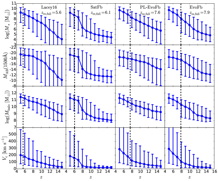
Figure 6: Simple statistics of the galaxies producing ionizing photons. Each column corresponds to a different SN feedback model, with the corresponding model name given in the top of each panel in the first row, along with the value of $z_{\rm re,full}$, the redshift at which the Universe is fully ionized. The vertical dashed lines in each panel also indicate $z_{\rm re,full}$. The first row shows the statistics of the stellar mass, $M_{*}$, of the galaxies producing ionizing photons, the second row shows the statistics of the dust-extincted rest frame UV magnitude, $M_{\rm AB}(1500{\rm\AA})$, of these galaxies, while the third row shows the statistics of the halo masses, $M_{\rm halo}$ and the fourth row shows the statistics of the galaxy circular velocity, $V_{\rm c}$. For each quantity shown in these rows, the dots indicate the medians of the corresponding quantity, and the errorbars the $5\--95\%$ range, with both the medians and the $5\--95\%$ ranges being determined by their contributions to the ionizing photon emissivity at that redshift.

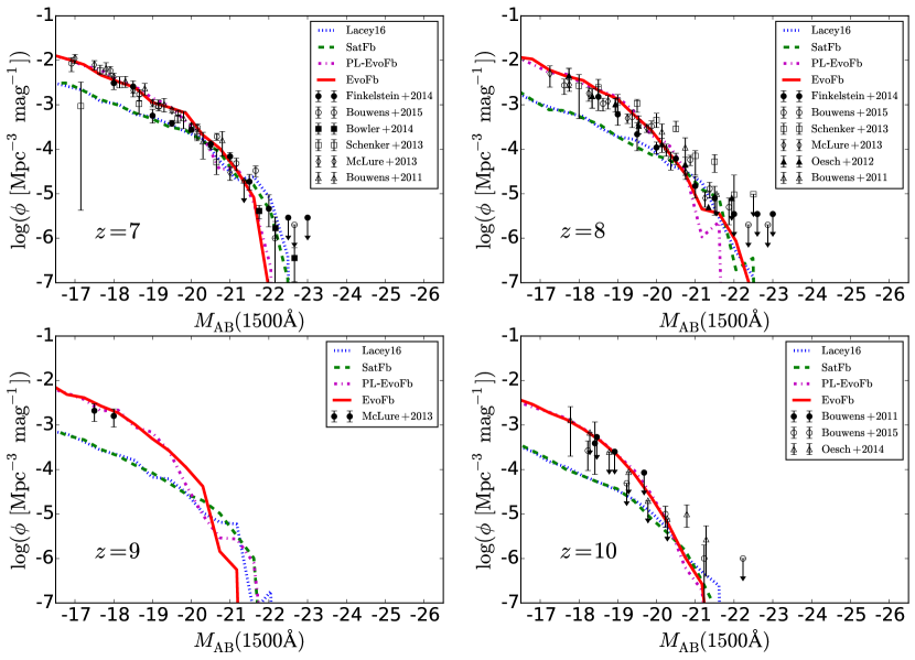
Figure 7: The rest frame far-UV luminosity functions at $z=7,\ 8,\ 9,\ 10$ for the 4 different SN feedback models. In each panel, the blue dotted line shows the prediction for the Lacey16 model, the dashed green line that for the SatFb model, the magenta dotted dashed line that for the PL-EvoFb model and the red solid line that for the EvoFb model, while symbols with errorbars indicate observational measurements (Bouwens et al., 2011b, a; Oesch et al., 2012; Schenker et al., 2013; McLure et al., 2013; Finkelstein et al., 2014; Bowler et al., 2014; Oesch et al., 2014; Bouwens et al., 2015). The dust extinction is calculated self-consistently based on galaxy gas content, size and metallicity (see Lacey et al. (2015) for more details).

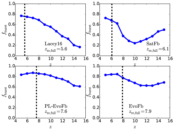
Figure 8: The fraction of the ionizing photon emissivity contributed by starbursts at a given redshift. Different panels are for different SN feedback models, as labelled, and the vertical dashed lines indicate $z_{\rm re,full}$.

Fig. 6 shows some simple statistics of the galaxies producing the ionizing photons. The first row shows the statistics of the stellar mass, $M_{*}$, of the galaxies producing ionizing photons, the second row shows the statistics of the dust-extincted rest-frame far-UV absolute magnitude, $M_{\rm AB}(1500{\rm\AA})$, of these galaxies, while the third row shows the statistics of the halo masses, $M_{\rm halo}$, and the fourth row the statistics of the galaxy circular velocity, $V_{\rm c}$. For each quantity, the dots in each panel indicate the medians of the corresponding quantity, and the error bars indicate the $5\--95\%$ range, with the medians and percentiles determined not by the number of galaxies but by their contributions to the ionizing emissivity at that redshift. The median means that galaxies below it contribute $50\%$ of the ionizing photons at a given redshift, while the $5\--95\%$ range indicates that the galaxies within it contribute $90\%$ of the ionizing photons at a given redshift. Each column corresponds to a different SN feedback model. The vertical dashed lines in each panel indicate $z_{\rm re,full}$, the redshift at which the Universe is fully ionized, for that model, with the numerical values of $z_{\rm re,full}$ given in the panels in the first row.

From Fig. 6 it is clear that the median of $M_{*}$ at $z\sim z_{\rm re,full}$ for each SN feedback model is around $10^{8}\--10^{9}\,{\rm M}_{\odot}$, the median of $M_{\rm AB}(1500{\rm\AA})$ is around $-17\---19$, and the median of $V_{\rm c}$ is around $100\--200\,{\rm km}\,{\rm s}^{-1}$. These values indicate that the corresponding galaxies are progenitors of large massive galaxies at $z=0$. This means in these models, the progenitors of large galaxies make significant contributions to the cosmic reionization. It is also true that the progenitors of large galaxies have already made contributions to the ionizing photons when the Universe was half ionized, i.e. by $z=z_{\rm re,half}$. This means that a preferential suppression of the SN feedback in very small galaxies is not very effective in boosting $z_{\rm re,half}$, and to predict a high enough $z_{\rm re,half}$ by these means usually requires heavy suppression of the SN feedback in very small galaxies, which spoils the agreement with observations of faint galaxies at $z=0$. This is the reason for the failure of the SatFb model to satisfy all the observational constraints considered in this work.

Fig. 6 also shows that the median of $M_{\rm halo}$ in each SN feedback model is roughly in the range $10^{10}\--10^{11}\,{\rm M}_{\odot}$ at $z\sim z_{\rm re,full}$, which means there are significant contributions to the ionizing photons from large atomic hydrogen cooling halos. This is consistent with the results from Boylan-Kolchin et al. (2014), who show that it is difficult to obtain reionization at $z\sim 8$ mainly from star formation in small atomic cooling halos with $M_{\rm halo}\sim 10^{8}\,{\rm M}_{\odot}$.

We also calculated the rest-frame far-UV luminosity functions at $z=7,\ 8,\ 9,\ 10$ for our 4 different SN feedback models. These predictions are shown in Fig. 7, and compared with recent observational data. The best fit (EvoFb) model is seen to agree quite well with the observations over the whole range $z=7\--10$. The PL-EvoFb model, which adopts similar redshift evolving SN feedback, also reaches similar level of agreement with observations. On the other hand, the other 2 models, which generally have stronger SN feedback at high redshift than the EvoFb model, predict too few low UV luminosity galaxies at $z=7\--10$. Note that the current observational limit is $M_{\rm AB}(1500{\rm\AA})\sim-17\---18$ at these redshifts, which is close to the median of $M_{\rm AB}(1500{\rm\AA})$ at reionization for the EvoFb model shown in Fig. 6 (for this model, at $z=8$, the median is $M_{\rm AB}(1500{\rm\AA})=-17.5$, and the $5\--95\%$ range is $M_{\rm AB}(1500{\rm\AA})=-12.1$ to $M_{\rm AB}(1500{\rm\AA})=-19.8$.). Thus the best fit model suggests that the currently observed high redshift galaxy population should contribute about half of the ionizing photons that reionized the Universe. This is consistent with Kuhlen & Faucher-Giguère (2012), which suggests that the sources of reionization can not be too heavily dominated by very faint galaxies.

We also checked that the rest-frame far-UV luminosity functions predicted by all 4 models become very similar at $z\leq 6$, and thus the modifications to the SN feedback do not spoil the good agreement of these luminosity functions with observations at $3\leq z\leq 6$ found in the original Lacey16 model.

Fig. 8 shows the fraction of the ionizing photons that are contributed by starbursts at a given redshift (as compared to stars formed quiescently in galaxy disks). Different panels are for different SN feedback models, and the vertical dashed lines indicate $z_{\rm re,full}$ for the corresponding models. It is clear that at $z\sim z_{\rm re,full}$, the starburst fractions are high, with $f_{\rm burst}\approx 0.8$ in all four models. This indicates that starbursts are a major source of the ionizing photons for cosmic reionization.

4.3 The descendants of the galaxies that ionized Universe

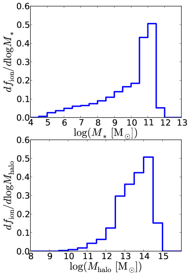
Figure 9: Probability distributions of masses of $z=0$ descendants of objects which emit ionizing photons at $z\geq z_{\rm re,full}$, weighted by number of ionizing photons produced. Upper panel: Probability distribution of stellar mass of descendant at $z=0$. Lower panel: Probability distribution of halo mass of descendant at $z=0$.

For the best fit model, i.e. the EvoFb model, we also identified the $z=0$ descendants of the galaxies which ionized the Universe. To do this, we ran a simulation with fixed dark matter halo mass resolution $M_{\rm res}=7.1\times 10^{7}\,{\rm M}_{\odot}$ from $z=20$ to $z=0$. This $M_{\rm res}$ is low enough to ensure that we resolve all the atomic cooling halos up to $z=11$. According to Fig. 3, most of the ionizing photons that reionized the Universe are produced near $z_{\rm re,full}$, and for the EvoFb model, $z_{\rm re,full}=7.9$. Thus, resolving all the atomic cooling halos up to $z=11$ ensures that all galaxies which are major sources of the ionizing photons and their star formation histories are well resolved.

In Fig. 9 we show the mass distributions of the $z=0$ descendants of the objects which produced the photons which reionized the Universe, weighted by the number of ionizing photons produced. The top panel shows the stellar mass of the descendant galaxy, while the bottom panel shows the mass of the descendant dark matter halo. To calculate these, we effectively identify each ionizing photon emitted at $z\geq z_{\rm re,full}$, then identify the $z=0$ descendant (galaxy or halo) of the galaxy which emitted it, then construct the probability distribution of descendant mass, giving equal weight to each ionizing photon. The upper panel of Fig. 9 shows that over $50\%$ of the ionizing photons are from the progenitors of large galaxies with $M_{*}>3\times 10^{10}\,{\rm M}_{\odot}$, or equivalently, the major ionizing sources have $z=0$ large galaxies as their descendants. The lower panel of Fig. 9 shows that $50\%$ of the ionizing photons are from the progenitors of high mass dark matter halos at $z=0$ with $M_{\rm halo}>3.7\times 10^{13}\,{\rm M}_{\odot}$, which means that the reionization is driven mainly by sources at very rare density peaks. These results are consistent with the indications given by Fig. 6.

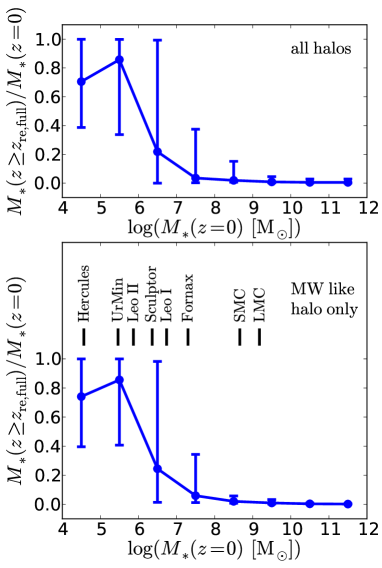
Figure 10: Fraction of stellar mass in galaxies at $z=0$ which was formed before reionization (i.e. at $z\geq z_{\rm re,full}$). In both panels, each filled circle shows the median of the ratio in the corresponding $z=0$ stellar mass bin, while the corresponding error bar indicates the $5\--95\%$ range of this ratio. Upper panel: All galaxies. Lower panel: Galaxies in Milky Way-like halos only (defined as halos with $z=0$ halo mass in the range $5\times 10^{11}\,{\rm M}_{\odot}\leq M_{\rm halo}\leq 2\times 10^{12}\,{\rm M}_{\odot}$). The short vertical solid black lines indicate the observed stellar masses of several Milky Way satellites, namely LMC, SMC, Fornax, Sculptor, Leo I, Leo II, Ursa Minor (UrMin) and Hercules, for reference (from McConnachie 2012).

In Fig. 10, we show the fraction of stellar mass in galaxies at $z=0$ that was formed before reionization, i.e. at $z\geq z_{\rm re,full}$, for the best fit model (the EvoFb model). The upper panel shows this for all galaxies, while the lower panel shows this quantity only for galaxies in Milky Way-like halos, defined as halos with $z=0$ halo mass in the range $5\times 10^{11}\,{\rm M}_{\odot}\leq M_{\rm halo}\leq 2\times 10^{12}\,{\rm M}_{\odot}$. The upper panel shows that even though the progenitors of the $z=0$ large galaxies provided about half of the ionizing photons, only a tiny fraction of their stars are formed before reionization, and while the $z=0$ dwarf galaxies ($M_{*}(z=0)<10^{6}\,{\rm M}_{\odot}$) contributed only a small fraction of the photons for reionization, their stellar populations typically are dominated by the stars formed before reionization. This is consistent with the hierarchical structure formation picture, because smaller objects formed earlier, and also formation of galaxies in small halos is suppressed after reionization by photoionization feedback. Also note that the ratio of the mass of the stars formed at $z\geq z_{\rm re,full}$ to the $z=0$ stellar mass shows considerable scatter for galaxies with $M_{*}(z=0)<10^{7}\,{\rm M}_{\odot}$, which means the star formation histories of these small galaxies are very diverse.

The lower panel of Fig. 10 shows galaxies in Milky Way-like halos only, but the predicted fraction of stars formed before reionization is in fact very similar to the average over all halos shown in the upper panel. For reference, the short vertical solid black lines indicate the observed stellar masses of several Milky Way satellites (from McConnachie 2012), namely LMC, SMC, Fornax, Sculptor, Leo I, Leo II, Ursa Minor (UrMin) and Hercules. As shown by this panel, the best fit model implies that for the large satellites like the LMC, SMC and Fornax, only tiny fractions of their stellar mass, typically 5% or less, were formed before reionization. However, this fraction increases dramatically with decreasing satellite mass, as does the scatter around the median. For the lowest mass satellites, with stellar mass $M_{*}<10^{6}\,{\rm M}_{\odot}$, including objects like Leo II, Ursa Minor and Hercules, the median fraction increases to around 80%, meaning that most of the satellites in this mass range form the bulk of their stars before reionization, with the 5–95% range in this fraction extending from 40% to 100%, indicating diverse star formation histories for different satellites of the same mass. Satellites in the intermediate mass range $10^{6}\,{\rm M}_{\odot}\leq M_{*}<10^{7}\,{\rm M}_{\odot}$, like Leo I and Sculptor, have somewhat lower median fractions formed before reionization, around 20–50%, but with an even larger scatter around this median, with the 5–95% range extending nearly from 0% to 100%.

4.4 Modelling uncertainties

An important assumption in our study is that $f_{\rm esc}$ is constant and, in our default model, equal to 0.2. This choice is justified in Section 2.3; here we explore the effects of varying this parameter. We also explore the effect of including a contribution from AGN to the photoionizing budget, which in our standard model we assume to be negligible.

Madau & Haardt (2015) have recently revived the old idea that photons produced by AGN could be responsible for reionization. They take the observed AGN Lyman limit emissivity, $\epsilon_{912}$, at $z\leq 6$ and extrapolate it to $z\approx 12$. Assuming that the AGN UV spectrum is a power law with index $-1.7$, they calculate the number of ionizing photons emitted by AGN per unit time per unit comoving volume, $\epsilon^{\prime}_{\rm AGN}$. The redshift of reionization can then be obtained either by solving the equation for $Q_{\rm HII}$, or using the simpler method we introduced in §2.3. Madau & Haardt (2015) conclude that AGN alone could have been the dominant source of the photons respsonsible for reionization.

The estimate of $\epsilon_{912}$ at $z\approx 6$ has a large errorbar and so a major uncertainty in the model of Madau & Haardt (2015) is their extrapolation to higher redshifts. They extrapolate using a complex functional form that, however, is close to an exponential, $\epsilon_{912}\propto\exp(\rm k_{\rm AGN}\,z)$, at $z\geq 5$, the regime relevant to hydrogen reionization. To assess the plausibility of the Madau & Haardt (2015) model, we investigate other extrapolations of $\epsilon_{912}$, which are consistent with the measured value at $z=6$. We consider the same exponential form, constrained in all cases to lie within the errorbar of the measured value at $z=6$ and to give the same value at $z=5$ as the Madau & Haardt (2015) model. (Unlike Madau & Haardt, for simplicity, we extrapolate to $z=\infty$ rather than to $z\approx 12$, as they do, but this overestimate of the AGN contribution introduces only very small changes to the redshift of reionization.) These two requirements result in a family of extrapolated estimates, with $-1.92\leq k_{\rm AGN}\leq-0.15$, illustrated by the grey shaded region in the upper left panel of Fig. 11. The emissivity assumed by Madau & Haardt (2015) lies at the upper boundary of this allowed region. Following Madau & Haardt we adopt an escape fraction of $100\%$ for AGN. There is considerable uncertainty on this parameter as well (see Madau & Haardt (2015) for further discussion).

Once $\epsilon^{\prime}_{\rm AGN}$ is known, the calculation in §2.3 can be extended to include AGN. Specifically, we have,

$$\epsilon_{\rm tot}(z) =f_{\rm esc}\epsilon_{\rm star}(z)+\epsilon_{\rm AGN}(z)$$ (9)

$${\cal R}^{\prime}(z) =\frac{\int_{z}^{\infty}\epsilon_{\rm tot}(z^{\prime})\,dz^{\prime}}{n_{\rm H}}$$ (10)

$${\cal R}^{\prime}(z_{\rm re,full}) =1+N_{\rm rec},$$ (11)

where $\epsilon_{\rm star}$ is the emissivity of the stars, which is given by galform, $f_{\rm esc}$ is the corresponding escape fraction, $n_{\rm H}$ is the comoving number density of hydrogen nuclei, $N_{\rm rec}=0.25$ is the mean number of recombinations per hydrogen nucleus up to $z_{\rm re,full}$, and $\epsilon_{\rm AGN}$ is the AGN photon emissivity per unit redshift, which is related to $\epsilon^{\prime}_{\rm AGN}$ by $\epsilon_{\rm AGN}=\epsilon^{\prime}_{\rm AGN}dt/dz$. The redshift of at which reionization is $50\%$ complete, $z_{\rm re,half}$, is calculated as in Eq(11), but for half the threshold. To explore the effect of different assumptions for $f_{\rm esc}$, we allow this parameter to vary in the range $0-0.25$.

Fig. 11 shows the effect of varying the AGN contribution (by varying $k_{\rm AGN}$) and $f_{\rm esc}$ on $z_{\rm re,half}$. We consider three models:  Lacey16, SatFb and EvoFb, as indicated in the corresponding legends. The contour lines show the predicted values of $z_{\rm re,half}$ in each model and the shaded area shows the region consistent with the Planck data. The PL-EvoFb model is not considered here because it is disfavoured by the MW satellite metallicity data.

As we have seen, stars in the Lacey16 model do not produce enough ionizing photons to reionize the Universe sufficiently early; AGN can reionize the Universe in this model but only if their emissivity has a very flat slope, $-0.25\leq k_{\rm AGN}\leq-0.15$; this extreme region is illustrated in the upper left panel of Fig. 11 as the red hatched area. The SatFb model also requires an AGN contribution in order to be consistent with the the values of $z_{\rm re,half}$ allowed by the Planck data, but this is generally less than required for the Lacey16 model. For our fiducial value of $f_{\rm esc}=0.2$, the required AGN emissivity corresponds to $-0.49\leq k_{\rm AGN}\leq-0.15$; this region is the blue hatched area in the upper left panel of Fig. 11. For lower values of $f_{\rm esc}$, the required range of $k_{\rm AGN}$ shrinks and comes close to the allowed upper limit. Finally, the EvoFb model is consistent with the Planck data in the case where all ionizing photons are produced by stars so long as $f_{\rm esc}\geq 0.07$; of course adding an AGN contribution makes it easier to reionize the Universe for even lower values of $f_{\rm esc}<0.07$.

In summary, even if AGN make a contribution to the ionizing photon budget, as long as $k_{\rm AGN}<-0.25$, our original, single power-law SN feedback model is incompatible with the Planck data. If $k_{\rm AGN}<-0.49$ and $f_{\rm esc}\geq 0.07$, then the evolving feedback model is preferred to the saturated feedback model, and our major conclusions regarding SN feedback still apply. Note that when $k_{\rm AGN}>-0.49$, the reionization redshift alone cannot discriminate between the SatFb and EvoFb models, but the measured far-UV galaxy luminosity functions at $z=7-10$ (Fig. 7) still prefer the evolving feedback model.

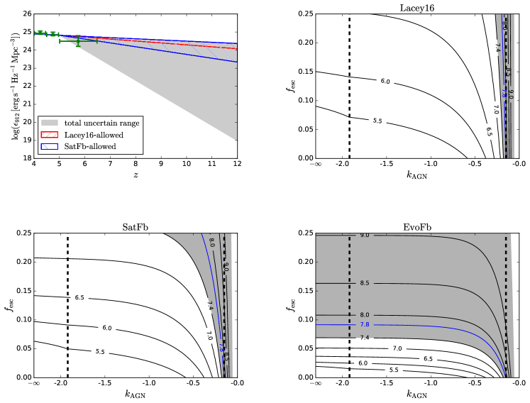
Figure 11: Upper left panel: extrapolations of the AGN emissivity at the Lyman limit, $\epsilon_{912}$, allowed by the errorbar of the measurement at $z\simeq 6$. The three data points with errorbars are the observations taken from Fig. 1 of Madau & Haardt (2015), the grey shaded region shows the allowed extrapolations. The extrapolation adopted by Madau & Haardt (2015) lies on the upper boundary of the region; the red and blue hatched regions encompass the extrapolations required to bring the Lacey16 and SatFb models respectively into agreement with the Planck constraints, for $f_{\rm esc}=0.2$. Reducing $f_{\rm esc}$ shrinks these regions towards the upper boundary. Remaining three panels: predicted $z_{\rm re,half}$ (contour lines) for different combinations of $f_{\rm esc}$ and $k_{\rm AGN}$, where $f_{\rm esc}$ is the escape fraction for stars and $k_{\rm AGN}$ is the slope of the AGN emissivity extrapolation shown in the upper left panel. The panels correspond to the Lacey16, SatFb and EvoFb models, as labelled. The grey shaded area in each panel represents the region allowed at $1$-$\sigma$ by the Planck data. The vertical dashed lines indicate the lower and upper limits of the extrapolation slope, i.e. $k_{\rm AGN}=-1.92$ and $k_{\rm AGN}=-0.15$. The line labelled $k_{\rm AGN}=-\infty$ corresponds to the case of no AGN contribution.

Our earlier conclusions regarding the sources of reionizing photons and their descendants are only valid when stars are the dominant source of reionizing photons. The contour lines in Fig. 12 show the fraction of the total ionizing photon budget produced by stars for different combinations of $f_{\rm esc}$ and $k_{\rm AGN}$. This photon budget includes all ionizing photons emitted from $z=\infty$ to $z_{\rm re,full}$. This is only shown for the EvoFb model, because this is our best-fit model and thus the most relevant to a discussion of reionization sources and their descendants. As the figure shows, so long as $f_{\rm esc}>0.07$ and $k_{\rm AGN}<-0.75$, over $90\%$ of the ionizing photons required for reionization come from stars; this fraction drops to $70\%$ if $k_{\rm AGN}=-0.49$, but is still dominant. Thus, our earlier conclusions regarding the reionization sources and their descendants remain valid so long as $f_{\rm esc}>0.07$ and $k_{\rm AGN}<-0.49$.

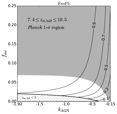
Figure 12: The fraction of ionizing photons from stars for different combinations of $f_{\rm esc}$ and $k_{\rm AGN}$ for our best-fit model, EvoFb. This photon budget includes all ionizing photons emitted from $z=\infty$ to $z_{\rm re,full}$. The fractions are shown as contour lines. The lower hatched region corresponds to $z_{\rm re,full}<5$ and is strongly excluded by other observations. The upper grey shaded region is allowed by the Planck data.

5 summary

We have investigated what constraints can be placed on supernova (SN) feedback by combining a physical model of galaxy formation with critical observations which constrain the strength of feedback in opposite directions. The observational constraints are: the optical and near-IR field luminosity functions (LFs) at $z=0$; the redshift $z_{\rm re,half}$, at which the Universe was half reionized; the Milky Way (MW) satellite LF; and the stellar metallicity vs. stellar mass ($Z_{*}\--M_{*}$) relation for MW satellites. We use the galform semi-analytical model of galaxy formation embedded in the $\Lambda$CDM model of structure formation, with 4 different formulations for the mass-loading factor, $\beta$, of galactic outflows driven by SN feedback: (a) in the Fiducial model, $\beta$ is a simple power law in galaxy circular velocity, $V_{\rm c}$; (b) in the Saturated feedback model, $\beta$ is a broken power law in $V_{\rm c}$, with a flat slope at low $V_{\rm c}$; (c) in the power law Evolving feedback model, $\beta$ is a single power law in $V_{\rm c}$, but with a normalization that is lower at higher redshifts; (d) in the Evolving feedback model, $\beta$ decreases at high redshift, as well as having a break to a shallower slope at low $V_{\rm c}$. The Fiducial model was previously tuned by Lacey et al. (2015) to fit a wide range of observational constraints, but not including reionization or the MW satellites. Our main conclusions are:

1. The single power law formulation of $\beta$ as used in the Fiducial model can reproduce the faint ends of the $z=0$ field LFs and MW satellite LF, but leads to too low $z_{\rm re,half}$ and too low MW satellite metallicities. This indicates that in this model, the SN feedback is too strong in small galaxies and/or at $z>8$.

2. Simply reducing the SN feedback in small galaxies, as in the Saturated model, does not provide an improvement relative to the single power law formulation of $\beta$.

3. The power law Evolving SN feedback model, with weaker SN feedback at high redshifts and stronger SN feedback at low redshifts, can successfully reproduce the faint ends of the $z=0$ field LFs, $z_{\rm re,half}$ and the MW satellite LF, but still predicts MW satellite metallicities that are too low, indicating the necessity of weakening the SN feedback in low $V_{\rm c}$ galaxies.

4. The Evolving SN feedback model, with the SN feedback strength decreasing with increasing redshift and a saturation for $V_{\rm c}\leq 50\,{\rm km}\,{\rm s}^{-1}$ , seems to be preferred by the above mentioned observational constraints. Including the effects of local reionization may further improve the predictions for the MW satellite LF.

5. The physical reasons for the redshift evolution in our phenomenological Evolving SN feedback models could be that a single function of galaxy $V_{\rm c}$ only captures the effects of the gravitational potential well on the SN feedback, but the SN feedback is likely also to depend on factors such as the cold gas density and metallicity and the molecular gas fraction, which evolve with redshift. However, a more detailed ISM model is required to test the conclusions from this work further.

6. In all of the SN feedback models analysed in this work, around 50% of the photons which reionize the IGM are emitted by galaxies with stellar masses $M_{*}\gtrsim 10^{9}\,{\rm M}_{\odot}$, rest-frame far-UV absolute magnitudes, $M_{\rm AB}(1500{\rm\AA})\lesssim-18$, galaxy circular velocities $V_{\rm c}\gtrsim 100\,{\rm km}\,{\rm s}^{-1}$ and halo masses $M_{\rm halo}\gtrsim 10^{11}\,{\rm M}_{\odot}$ at the redshift $z\sim z_{\rm re,full}$ at which the Universe is fully reionized. In addition, most of the ionizing photons are predicted to be emitted by galaxies undergoing starbursts, rather than forming stars quiescently. This implies that the currently observed high redshift galaxy population should contribute about half of the ionizing photons that reionized Universe.

7. For our best fit model, namely the Evolving feedback model, the $z=0$ descendants of the major ionizing photon sources are relatively large galaxies with $M_{*}\gtrsim 10^{10}\,{\rm M}_{\odot}$, and are mainly in dark matter halos with $M_{\rm halo}\gtrsim 10^{13}\,{\rm M}_{\odot}$. However, for these galaxies, the fraction of stars formed before reionization is low, while this fraction is high for dwarf galaxies with $z=0$ stellar masses $M_{*}<10^{6}\,{\rm M}_{\odot}$, even though the progenitors of such dwarfs contribute little to reionizing the Universe. This fraction also shows considerable scatter for the dwarfs, indicating that the star formation histories of these dwarf galaxies are very diverse.

8. For satellite galaxies in Milky Way-like halos, our best fit model implies that the fraction of stars formed before reionization is very low for large satellites like the LMC, SMC and Fornax, but reaches very high values for very small satellites with stellar masses $M_{*}<10^{6}\,{\rm M}_{\odot}$, like Leo II, Ursa Minor and Hercules, with median fractions around $80\%$, indicating that typically these small satellites formed most of their stars before reionization.

References

- Alexandroff et al. (2015) Alexandroff R. M., Heckman T. M., Borthakur S., Overzier R., Leitherer C., 2015, ApJ, 810, 104
- Asplund et al. (2009) Asplund M., Grevesse N., Sauval A. J., Scott P., 2009, ARA&A, 47, 481
- Bate (2012) Bate M. R., 2012, MNRAS, 419, 3115
- Baugh et al. (2005) Baugh C. M., Lacey C. G., Frenk C. S., Granato G. L., Silva L., Bressan A., Benson A. J., Cole S., 2005, MNRAS, 356, 1191
- Benson et al. (2003) Benson A. J., Bower R. G., Frenk C. S., Lacey C. G., Baugh C. M., Cole S., 2003, ApJ, 599, 38
- Benson et al. (2002) Benson A. J., Lacey C. G., Baugh C. M., Cole S., Frenk C. S., 2002, MNRAS, 333, 156
- Borthakur et al. (2014) Borthakur S., Heckman T. M., Leitherer C., Overzier R. A., 2014, Science, 346, 216
- Bouwens et al. (2011a) Bouwens R. J. et al., 2011a, Nature, 469, 504
- Bouwens et al. (2011b) Bouwens R. J. et al., 2011b, ApJ, 737, 90
- Bouwens et al. (2015) Bouwens R. J. et al., 2015, ApJ, 803, 34
- Bower et al. (2006) Bower R. G., Benson A. J., Malbon R., Helly J. C., Frenk C. S., Baugh C. M., Cole S., Lacey C. G., 2006, MNRAS, 370, 645
- Bowler et al. (2014) Bowler R. A. A. et al., 2014, MNRAS, 440, 2810
- Boylan-Kolchin et al. (2014) Boylan-Kolchin M., Bullock J. S., Garrison-Kimmel S., 2014, MNRAS, 443, L44
- Cole et al. (2000) Cole S., Lacey C. G., Baugh C. M., Frenk C. S., 2000, MNRAS, 319, 168
- Couchman & Rees (1986) Couchman H. M. P., Rees M. J., 1986, MNRAS, 221, 53
- Davé et al. (2013) Davé R., Katz N., Oppenheimer B. D., Kollmeier J. A., Weinberg D. H., 2013, MNRAS, 434, 2645
- de Boer et al. (2012) de Boer T. J. L. et al., 2012, A&A, 544, A73
- Dekel & Silk (1986) Dekel A., Silk J., 1986, ApJ, 303, 39
- Driver et al. (2012) Driver S. P. et al., 2012, MNRAS, 427, 3244
- Efstathiou (1992) Efstathiou G., 1992, MNRAS, 256, 43P
- Finkelstein et al. (2014) Finkelstein S. L. et al., 2014, ArXiv:1410.5439
- Finlator et al. (2012) Finlator K., Oh S. P., Özel F., Davé R., 2012, MNRAS, 427, 2464
- Font et al. (2011) Font A. S. et al., 2011, MNRAS, 417, 1260
- Fontanot et al. (2012) Fontanot F., Cristiani S., Vanzella E., 2012, MNRAS, 425, 1413
- Giallongo et al. (2015) Giallongo E. et al., 2015, A&A, 578, A83
- Haardt & Madau (2012) Haardt F., Madau P., 2012, ApJ, 746, 125
- Hopkins et al. (2012) Hopkins P. F., Quataert E., Murray N., 2012, MNRAS, 421, 3488
- Kimm & Cen (2014) Kimm T., Cen R., 2014, ApJ, 788, 121
- Klypin et al. (1999) Klypin A., Kravtsov A. V., Valenzuela O., Prada F., 1999, ApJ, 522, 82
- Komatsu et al. (2011) Komatsu E. et al., 2011, ApJS, 192, 18
- Koposov et al. (2008) Koposov S. et al., 2008, ApJ, 686, 279
- Kuhlen & Faucher-Giguère (2012) Kuhlen M., Faucher-Giguère C.-A., 2012, MNRAS, 423, 862
- Lacey et al. (2015) Lacey C. G. et al., 2015, ArXiv:1509.08473
- Lagos et al. (2013) Lagos C. d. P., Lacey C. G., Baugh C. M., 2013, MNRAS, 436, 1787
- Larson (1974) Larson R. B., 1974, MNRAS, 169, 229
- Lewis (2008) Lewis A., 2008, Phys. Rev. D, 78, 023002
- Madau & Haardt (2015) Madau P., Haardt F., 2015, ApJ, 813, L8
- Madau et al. (1999) Madau P., Haardt F., Rees M. J., 1999, ApJ, 514, 648
- McConnachie (2012) McConnachie A. W., 2012, AJ, 144, 4
- McLure et al. (2013) McLure R. J. et al., 2013, MNRAS, 432, 2696
- Moore et al. (1999) Moore B., Ghigna S., Governato F., Lake G., Quinn T., Stadel J., Tozzi P., 1999, ApJ, 524, L19
- Norberg et al. (2002) Norberg P. et al., 2002, MNRAS, 336, 907
- Oesch et al. (2012) Oesch P. A. et al., 2012, ApJ, 759, 135
- Oesch et al. (2014) Oesch P. A. et al., 2014, ApJ, 786, 108
- Okamoto et al. (2008) Okamoto T., Gao L., Theuns T., 2008, MNRAS, 390, 920
- Paardekooper et al. (2015) Paardekooper J.-P., Khochfar S., Dalla Vecchia C., 2015, MNRAS, 451, 2544
- Parkinson et al. (2008) Parkinson H., Cole S., Helly J., 2008, MNRAS, 383, 557
- Planck Collaboration et al. (2014) Planck Collaboration et al., 2014, A&A, 571, A16
- Planck Collaboration et al. (2015) Planck Collaboration et al., 2015, ArXiv:1502.01589
- Raičević et al. (2011) Raičević M., Theuns T., Lacey C., 2011, MNRAS, 410, 775
- Schaye et al. (2015) Schaye J. et al., 2015, MNRAS, 446, 521
- Schenker et al. (2013) Schenker M. A. et al., 2013, ApJ, 768, 196
- Sharma et al. (2016) Sharma M., Theuns T., Frenk C., Bower R., Crain R., Schaller M., Schaye J., 2016, MNRAS, 458, L94
- Shull et al. (2012) Shull J. M., Harness A., Trenti M., Smith B. D., 2012, ApJ, 747, 100
- Thoul & Weinberg (1996) Thoul A. A., Weinberg D. H., 1996, ApJ, 465, 608
- Vanzella et al. (2010) Vanzella E. et al., 2010, ApJ, 725, 1011
- Vargas et al. (2013) Vargas L. C., Geha M., Kirby E. N., Simon J. D., 2013, ApJ, 767, 134
- Vogelsberger et al. (2014) Vogelsberger M. et al., 2014, Nature, 509, 177
- White & Frenk (1991) White S. D. M., Frenk C. S., 1991, ApJ, 379, 52