Constraining top quark effective theory
in the LHC Run II era

Abstract

We perform an up-to-date global fit of top quark effective theory to experimental data from the Tevatron, and from LHC Runs I and II. Experimental data includes total cross-sections up to 13 TeV, as well as differential distributions, for both single top and pair production. We also include the top quark width, charge asymmetries, and polarisation information from top decay products. We present bounds on the coefficients of dimension six operators, and examine the interplay between inclusive and differential measurements, and Tevatron / LHC data. All results are currently in good agreement with the Standard Model.

GLAS-PPE/2015-08

1 Introduction

One of the primary goals of the Large Hadron Collider (LHC) is to uncover the precise mechanism responsible for electroweak symmetry breaking. Going beyond its ad hoc implementation in the Standard Model (SM), most realisations of this mechanism predict that new, possibly non-resonant physics will appear at the (multi-)TeV scale. Faced with the large number of such scenarios, and the frequent degeneracy in their experimental signatures, it has become customary to parametrize deviations of LHC measurements from their Standard Model predictions in terms of model-independent parameters, where possible. In Higgs production, for instance, the deviations in early inclusive cross-section measurements are described by ‘signal strength’ ratios. Likewise, deviations in electroweak parameters are often expressed in the language of anomalous couplings.

With the LHC Run I at a close, the main message to be drawn is that, apart from a few scattered anomalies, all measurements are in agreement with Standard Model predictions. This suggests that the new degrees of freedom, if they exist at all, are separated in mass [1, 2] from the Standard Model fields. If this is true, the new physics can be modelled by an infinite series of higher-dimensional effective operators [4, 5, 6, 7]. From a phenomenological perspective, these have the advantage over simple signal strengths in that they can also accommodate differential measurements and angular observables, since the operators lead to new vertex structures which modify event kinematics. They are also preferable to anomalous couplings since they preserve the Standard Model $SU(3)_{C}\times SU(2)_{L}\times U(1)_{Y}$ gauge symmetry, so can more easily be linked to ultraviolet completions than arbitrary form factors. These merits have not gone unnoticed, as effective field theory (EFT) techniques have received much attention in interpreting available Higgs results [8, 9, 10, 11, 12, 13, 14, 15, 16, 17, 18, 19, 20, 21, 22, 23, 24, 25]. This area, however, is still in its infancy, as such analyses are currently limited on the experimental side by low statistics.

Top quark physics, on the other hand, has entered a precision era, with data from the LHC and Tevatron far more abundant. In addition, the top quark plays a special role in most scenarios of Beyond the Standard Model physics, motivating scrutiny of its phenomenology. Furthermore, the top sector is strongly coupled to Higgs physics owing to the large top quark Yukawa coupling, and so represents a complementary window into physics at the electroweak scale. Thus, it is timely to compute the constraints on new top interactions through a global fit of all dimension-six operators relevant to top production and decay at hadron colliders.

There have been several studies of the potential for uncovering new physics effects in the top quark sector at the LHC and Tevatron, phrased in model-independent language, either through anomalous couplings [26, 27, 28, 29, 30, 31, 32, 33, 34, 35, 36, 37, 38, 39, 40, 41] or higher-dimensional operators [42, 43, 44, 45, 46, 47, 48]. Though there is a one-to-one correspondence between these two approaches (for the reasons discussed below) the latter is the approach taken through the rest of this paper. Other studies have also set limits on top dimension-six operators, but by considering different physics, such as precision electroweak data [49], or flavour-changing neutral currents [50, 51].

In a previous work [52], we published constraints on all dimension-six operators that contribute to top pair and single top production only in a global fit. Our fitting approach used techniques borrowed from Monte Carlo event generator tuning, namely the Professor [53] framework. The purpose of this paper is to expand on our previous study by adding new measurements, which are sensitive to a new set of operators not previously examined, including previously unreleased 8 and 13 TeV data and decay observables, and also to provide a more detailed review of our general fitting procedure.

The paper is structured as follows. In Section 2 we review the higher-dimensional operators relevant for top quark physics and in Section 3 we review the experimental measurements entering our fit, as well as the limit-setting procedure we adopt. In Section 4 we present our constraints, and discuss the complementarity of LHC and Tevatron analyses, and the improvements obtained from adding differential distributions as well as inclusive rates. In Section 5 we interpret our constraints in the context of two specific new physics models. Finally, in Section 6 we discuss our results and conclude.

2 Higher-dimensional operators

In effective field theory language, the Standard Model Lagrangian is the first term in an effective Lagrangian

$$\mathcal{L}_{\mathrm{eff}}=\mathcal{L}_{\mathrm{SM}}+\frac{1}{\Lambda}\mathcal{L}_{1}+\frac{1}{\Lambda^{2}}\mathcal{L}_{2}+\ldots\,,$$ (1)

where $\Lambda$ generically represents the scale of the new physics. From a top-down viewpoint, the higher-dimensional terms that are suppressed by powers of $1/\Lambda$ originate from heavy degrees of freedom that have been integrated out. In this way, the low-energy effects of decoupled new physics can be captured, without the need to consign oneself to a particular ultraviolet model. The leading contributions to $\mathcal{L}_{\mathrm{eff}}$ at collider energies enter at dimension-six

$$\mathcal{L}_{\mathrm{eff}}=\mathcal{L}_{\mathrm{SM}}+\frac{1}{\Lambda^{2}}\sum_{i}C_{i}O_{i}(G^{a}_{\mu},W^{I}_{\mu},B_{\mu},\varphi,q_{L},u_{R},d_{R},l_{L},e_{R})+\mathcal{O}(\Lambda^{-4})\,.$$ (2)

$O_{i}$ are dimension-six operators made up of SM fields, and $C_{i}$ are dimensionless Wilson coefficients. At dimension-six, assuming minimal flavour violation and Baryon number conservation, there are 59 independent operators. Clearly, allowing 59 free parameters to float in a global fit is intractable. Fortunately, for any given class of observables, only a smaller subset is relevant. In top physics, we have the following effective operators, expressed in the so-called ‘Warsaw basis’ of Ref. [54]

$$O^{(1)}_{qq} =(\bar{q}\gamma_{\mu}q)(\bar{q}\gamma^{\mu}q) O_{uW} =(\bar{q}\sigma^{\mu\nu}\tau^{I}u)\tilde{\varphi}W_{\mu\nu}^{I} O^{(3)}_{\varphi q} =i(\varphi^{\dagger}\overleftrightarrow{D}^{I}_{\mu}\varphi)(\bar{q}\gamma^{\mu}\tau^{I}q)$$

$$O^{(3)}_{qq} =(\bar{q}\gamma_{\mu}\tau^{I}q)(\bar{q}\gamma^{\mu}\tau^{I}q) O_{uG} =(\bar{q}\sigma^{\mu\nu}T^{A}u)\tilde{\varphi}G_{\mu\nu}^{A} O^{(1)}_{\varphi q} =i(\varphi^{\dagger}\overleftrightarrow{D}_{\mu}\varphi)(\bar{q}\gamma^{\mu}q)$$

$$O_{uu} =(\bar{u}\gamma_{\mu}u)(\bar{u}\gamma^{\mu}u) O_{G} =f_{ABC}G_{\mu}^{A\nu}G_{\nu}^{B\lambda}G_{\lambda}^{C\mu} O_{uB} =(\bar{q}\sigma^{\mu\nu}u)\tilde{\varphi}B_{\mu\nu}$$

$$O^{(8)}_{qu} =(\bar{q}\gamma_{\mu}T^{A}q)(\bar{u}\gamma^{\mu}T^{A}u) O_{\tilde{G}} =f_{ABC}\tilde{G}_{\mu}^{A\nu}G_{\nu}^{B\lambda}G_{\lambda}^{C\mu} O_{\varphi u} =(\varphi^{\dagger}i\overleftrightarrow{D}_{\mu}\varphi)(\bar{u}\gamma^{\mu}u)$$

$$O^{(8)}_{qd} =(\bar{q}\gamma_{\mu}T^{A}q)(\bar{d}\gamma^{\mu}T^{A}d) O_{\varphi G} =(\varphi^{\dagger}\varphi)G_{\mu\nu}^{A}G^{A\mu\nu} O_{\varphi\tilde{G}} =(\varphi^{\dagger}\varphi)\tilde{G}_{\mu\nu}^{A}G^{A\mu\nu}$$

$$O^{(8)}_{ud} =(\bar{u}\gamma_{\mu}T^{A}u)(\bar{d}\gamma^{\mu}T^{A}d)\,.$$ (3)

We adopt the same notation as Ref. [54], where $T^{A}=\tfrac{1}{2}\lambda^{A}$ are the $SU(3)$ generators, and $\tau^{I}$ are the Pauli matrices, related to the generators of $SU(2)$ by $S^{I}=\tfrac{1}{2}\tau^{I}$. For the four-quark operators on the left column of eq. (3), we denote a specific flavour combination $(\bar{q}_{i}...q_{j})(\bar{q}_{k}...q_{l})$ by e.g. $O_{4q}^{ijkl}$. It should be noted that the operators $O_{uW}$, $O_{uG}$ and $O_{uB}$ are not hermitian and so may have complex coefficients which, along with $O_{\tilde{G}}$ and $O_{\varphi\tilde{G}}$, lead to $\mathcal{CP}$-violating effects. These do not contribute to Standard Model spin-averaged cross-sections, though they are in principle sensitive to polarimetric observables such as spin correlations, and should therefore be treated as independent operators. However, currently available measurements that would be sensitive to these degrees of freedom have been extracted by making model-specific assumptions that preclude their usage in our fit, e.g. by assuming that the tops are produced with either SM-like spin correlation or no spin correlation at all, as in Refs. [61, 62]. We will discuss this issue in more detail in the next section. With these caveats, a total of 14 constrainable $\mathcal{CP}$-even dimension-six operators contribute to top quark production and decay at leading order in the SMEFT.

3 Methodology

3.1 Experimental inputs

The experimental measurements used in the fit [63, 64, 65, 66, 67, 68, 69, 70, 71, 72, 73, 74, 75, 76, 77, 78, 79, 80, 81, 82, 83, 84, 85, 86, 87, 88, 89, 90, 91, 92, 93, 94, 95, 96, 97, 98, 99, 100] are included in Table 1. All these measurements are quoted in terms of ‘parton-level’ quantities; that is, top quarks and their direct decay products. Whilst it is possible to include particle-level observables, these are far less abundant and they are beyond the scope of the present study.

The importance of including kinematic distributions is manifest here. For top pair production, for instance, we have a total of 195 measurements, 174 of which come from differential observables. This size of fit is unprecedented in top physics, which underlines the need for a systematic fitting approach, as provided by Professor. Indeed top pair production cross-sections make up the bulk of measurements that are used in the fit. Single top production cross-sections comprise the next dominant contribution. We also make use of data from charge asymmetries in top pair production, as well as inclusive measurements of top pair production in association with a photon or a $Z$ ($t\bar{t}\gamma$ and $t\bar{t}Z$) and observables relating to top quark decay. We take each of these categories of measurement in turn, discussing which operators are relevant and the constraints obtained on them from data.

Dataset $\sqrt{s}$ (TeV) Measurements arXiv ref. Dataset $\sqrt{s}$ (TeV) Measurements arXiv ref. Top pair production Total cross-sections: Differential cross-sections: ATLAS 7 lepton+jets 1406.5375 ATLAS 7 $p_{T}(t),M_{t\bar{t}},|y_{t\bar{t}}|$ 1407.0371 ATLAS 7 dilepton 1202.4892 CDF 1.96 $M_{t\bar{t}}$ 0903.2850 ATLAS 7 lepton+tau 1205.3067 CMS 7 $p_{T}(t),M_{t\bar{t}},y_{t},y_{t\bar{t}}$ 1211.2220 ATLAS 7 lepton w/o $b$ jets 1201.1889 CMS 8 $p_{T}(t),M_{t\bar{t}},y_{t},y_{t\bar{t}}$ 1505.04480 ATLAS 7 lepton w/ $b$ jets 1406.5375 D${\not{0}}$ 1.96 $M_{t\bar{t}},p_{T}(t),|y_{t}|$ 1401.5785 ATLAS 7 tau+jets 1211.7205 ATLAS 7 $t\bar{t},Z\gamma,WW$ 1407.0573 Charge asymmetries: ATLAS 8 dilepton 1202.4892 ATLAS 7 $A_{\mathrm{C}}$ (inclusive+$M_{t\bar{t}},y_{t\bar{t}}$) 1311.6742 CMS 7 all hadronic 1302.0508 CMS 7 $A_{\mathrm{C}}$ (inclusive+$M_{t\bar{t}},y_{t\bar{t}}$) 1402.3803 CMS 7 dilepton 1208.2761 CDF 1.96 $A_{\mathrm{FB}}$ (inclusive+$M_{t\bar{t}},y_{t\bar{t}}$) 1211.1003 CMS 7 lepton+jets 1212.6682 D${\not{0}}$ 1.96 $A_{\mathrm{FB}}$ (inclusive+$M_{t\bar{t}},y_{t\bar{t}}$) 1405.0421 CMS 7 lepton+tau 1203.6810 CMS 7 tau+jets 1301.5755 Top widths: CMS 8 dilepton 1312.7582 D${\not{0}}$ 1.96 $\Gamma_{\!\mathrm{top}}$ 1308.4050 CDF + D${\not{0}}$ 1.96 Combined world average 1309.7570 CDF 1.96 $\Gamma_{\!\mathrm{top}}$ 1201.4156 Single top production $W$​-boson helicity fractions: ATLAS 7 $t$-channel (differential) 1406.7844 ATLAS 7 1205.2484 CDF 1.96 $s$-channel (total) 1402.0484 CDF 1.96 1211.4523 CMS 7 $t$-channel (total) 1406.7844 CMS 7 1308.3879 CMS 8 $t$-channel (total) 1406.7844 D${\not{0}}$ 1.96 1011.6549 D${\not{0}}$ 1.96 $s$-channel (total) 0907.4259 D${\not{0}}$ 1.96 $t$-channel (total) 1105.2788 Associated production Run II data ATLAS 7 $t\bar{t}\gamma$ 1502.00586 CMS 13 $t\bar{t}$ (dilepton) 1510.05302 ATLAS 8 $t\bar{t}Z$ 1509.05276 CMS 8 $t\bar{t}Z$ 1406.7830

Table 1: The measurements entering our fit. Details of each are described in the text.

3.2 Treatment of uncertainties

The uncertainties entering our fit can be classed into three categories:

Experimental uncertainties:

We generally have no control over these. In cases where statistical and systematic (and luminosity) errors are recorded separately, we add them in quadrature. Correlations between measurements are also an issue: the unfolding of measured distributions to parton-level introduces some correlation between neighbouring bins. If estimates of these effects have been provided in the experimental analysis, we use this information in the fit, if they are not, we assume zero correlation. However, we have checked that bin correlations have little effect on our numerical results.

There will also be correlations between apparently separate measurements. The multitude of different top pair production cross-section measurements will clearly be correlated due to overlapping event selection criteria and detector effects, etc. Without a full study of the correlations between different decay channels measured by the same experiment, these effects cannot be completely taken into account, but based on the negligible effects of the bin-by-bin correlations on our numerical results we can expect these effects to be small as well.

Standard Model theoretical uncertainties:

These stem from the choice of parton distribution functions (PDFs), as well as neglected higher-order perturbative corrections. As is conventional, we model the latter by varying the renormalisation and factorisation scales independently in the range $\mu_{0}/2\leq\mu_{\mathrm{R,F}}\leq 2\mu_{0}$, where we use $\mu_{0}=m_{t}$ as the default scale, and take the envelope as our uncertainty. For the PDF uncertainty, we follow the PDF4LHC recommendation [101] of using CT10 [102], MSTW [103] & NNPDF [104] NLO fits, each with associated scale uncertainties, then taking the full width of the scale+PDF envelope as our uncertainty estimate – i.e. we conservatively assume that scales and parton densities are 100% correlated. Unless otherwise stated, we take the top quark mass to be $m_{t}=173.2\pm 1.0~{}\text{G}\mspace{0.2mu}\text{e}\mspace{-1.0mu}\text{V}$. We do not consider electroweak corrections.

Only recently a lot of progress has been made in extending the dimension six-extended SM to higher order, see Refs. [105, 106, 107, 108, 109, 110, 111, 112, 113, 114, 115, 116, 117, 118]. Including these effects is beyond the scope of this work, also because we work to leading order accuracy in the electroweak expansion of the SM. QCD corrections to four fermion operators included via renormalisation group equations are typically of the order of 15%, depending on the resolved phase space [114]. As pointed out in Ref. [119], these effects can be important in electroweak precision data fits.

Interpolation error:

A small error relating to the Monte Carlo interpolation (described in more detail in the next section) is included. This is estimated to be 5% at a conservative estimate, as discussed in the following section, and subleading compared to the previous two categories.

3.3 Fitting procedure

Our fitting procedure, briefly outlined in Ref. [52], uses the Professor framework. The first step is to construct an $N$-dimensional hypercube in the space of dimension six couplings, compute the observables at each point in the space, and then to fit an interpolating function $f(\mathbf{C})$ that parametrises the theory prediction as a function of the Wilson coefficients $\mathbf{C}=\{C_{i}\}$. This can then be used to rapidly generate theory observables for arbitrary values of the coefficients. Motivated by the dependence of the total cross-section with a Wilson coefficient:

$$\sigma\sim\sigma_{\mathrm{SM}}+C_{i}\sigma_{D6}+C^{2}_{i}\sigma_{D6^{2}}\,,$$ (4)

the fitting function is chosen to be a second-order or higher polynomial:

$$f_{b}(\{C_{i}\})=\alpha_{0}^{b}+\sum_{\begin{subarray}{c}i\end{subarray}}\beta_{i}^{b}C_{i}+\sum_{\begin{subarray}{c}i\leq j\end{subarray}}\gamma^{b}_{i,j}C_{i}C_{j}+\ldots\,.$$ (5)

Figure 1: Residuals distributions for interpolated observable values (left) and uncertainties (right), evaluated over all input MC runs and all observables. The 4th order polynomial parameterisation gives the best performance and the vast majority of entries are within 5% of the explicit MC value. The poor performance of a constant uncertainty assumption based on the median input uncertainty is evident – since all three lines have the same normalisation, the majority of residual mismodellings for the median approach are (far) outside the displayed 10% interval.

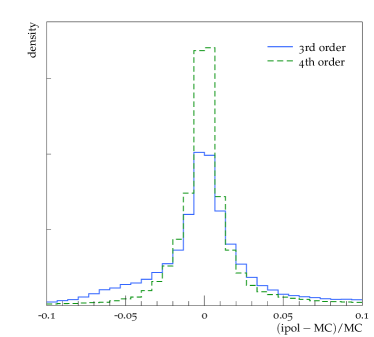
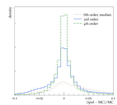
In the absence of systematic uncertainties, each observable would exactly follow a second-order polynomial in the coefficients, and higher-order terms capture bin uncertainties which modify this. The polynomial also serves as a useful check that the dimension-six approximation is valid. By comparing eq. (4) with eq. (5), we see that the terms quadratic in $C_{i}$ are small provided that the coefficients in the interpolating function $\gamma_{i,j}$ are small. This is a more robust way to ensure validity of the dimension-six approximation than to assume a linear fit from the start.

In practice, to minimise the interpolation uncertainty, we use up to a 4th order polynomial in eq. (5), depending on the observable of interest. The performance of the interpolation method is shown in Figure 1, which depicts the fractional deviation of the polynomial fit from the explicit MC points used to constrain it. The central values and the sizes of the modelling uncertainties may both be parameterised with extremely similar performance, with 4th order performing best for both. The width of this residual mismodeling distribution being $\sim\text{3\%}$ for each of the value and error components is the motivation for a total 5% interpolation uncertainty to be included in the goodness of fit of the interpolated MC polynomial $f(\mathbf{C})$ to the experimentally measured value $E$:

$$\chi^{2}(\mathbf{C})=\sum_{\begin{subarray}{c}\mathcal{O}\end{subarray}}\sum_{\begin{subarray}{c}i,j\end{subarray}}\frac{(f_{i}(\mathbf{C})-E_{i})\rho_{i,j}(f_{j}(\mathbf{C})-E_{j})}{\sigma_{i}\sigma_{j}}\,,$$ (6)

where we sum over all observables $\mathcal{O}$ and all bins in that observable $i$. We include the correlation matrix $\rho_{i,j}$ where this is provided by the experiments, otherwise $\rho_{i,j}=\delta_{ij}$. The uncertainty on each bin is given by $\sigma_{i}=\sqrt{\sigma_{\mathrm{th},i}^{2}+\sigma_{\mathrm{exp},i}^{2}}$, i.e. we treat theory and experimental errors as uncorrelated. The parameterisation of the theory uncertainties is restricted to not become larger than in the training set, to ensure that polynomial blow-up of the uncertainty at the edges of the sampling range cannot produce a spuriously low $\chi^{2}$ and disrupt the fit.

We hence have constructed a fast parameterisation of model goodness-of-fit as a function of the EFT operator coefficients. This may be used to produce $\chi^{2}$ maps in slices or marginalised projections of the operator space, which are then transformed to confidence intervals on the coefficients $C_{i}$, defined by the regions for which

$$1-\mathrm{CL}\geq\int^{\infty}_{\chi^{2}(C_{i})}f_{k}(x)dx\,,$$ (7)

where typically $\mathrm{CL}\in\{0.68,0.95,0.99\}$ and $f_{k}(x)$ is the $\chi^{2}$ distribution for $k$ degrees of freedom, which we define as $k=N_{\mathrm{measurements}}-N_{\mathrm{coefficients}}$.

4 Results

The entire 59 dimensional operator set of Ref. [54] was implemented in a FeynRules [120] model file. The contributions to parton level cross-sections and decay observables from the above operators were computed using MadGraph/Madevent [121], making use of the Universal FeynRules Output (UFO) [122] format. We model NLO QCD corrections by including Standard Model $K$-factors (bin-by-bin for differential observables), where the NLO observables are calculated using MCFM [123], cross-checked with MC@NLO [124, 125]. These $K$-factors are used for arbitrary values of the Wilson coefficients, thus modelling NLO effects in the pure-SM contribution only. More specifically, this amounts to performing a simultaneous expansion of each observable in the strong coupling $\alpha_{s}$ and the (inverse) new physics scale $\Lambda^{-1}$, and neglecting terms $\sim{\cal O}(\alpha_{S}\Lambda^{-2})$. Our final 95% confidence limits for each coefficient are presented in Figure 12; we discuss them in more detail below.

4.1 Top pair production

By far the most abundant source of data in top physics is from the production of top pairs. The $\mathcal{CP}$-even dimension-six operators that interfere with the Standard Model amplitude are

$$\begin{split}\mathcal{L}_{D6}&\supset\frac{C_{uG}}{\Lambda^{2}}(\bar{q}\sigma^{\mu\nu}T^{A}u)\tilde{\varphi}G_{\mu\nu}^{A}+\frac{C_{G}}{\Lambda^{2}}f_{ABC}G_{\mu}^{A\nu}G_{\nu}^{B\lambda}G_{\lambda}^{C\mu}+\frac{C_{\varphi G}}{\Lambda^{2}}(\varphi^{\dagger}\varphi)G_{\mu\nu}^{A}G^{A\mu\nu}\\ &+\frac{C^{(1)}_{qq}}{\Lambda^{2}}(\bar{q}\gamma_{\mu}q)(\bar{q}\gamma^{\mu}q)+\frac{C^{(3)}_{qq}}{\Lambda^{2}}(\bar{q}\gamma_{\mu}\tau^{I}q)(\bar{q}\gamma^{\mu}\tau^{I}q)+\frac{C_{uu}}{\Lambda^{2}}(\bar{u}\gamma_{\mu}u)(\bar{u}\gamma^{\mu}u)\\ &+\frac{C^{(8)}_{qu}}{\Lambda^{2}}(\bar{q}\gamma_{\mu}T^{A}q)(\bar{u}\gamma^{\mu}T^{A}u)+\frac{C^{(8)}_{qd}}{\Lambda^{2}}(\bar{q}\gamma_{\mu}T^{A}q)(\bar{d}\gamma^{\mu}T^{A}d)+\frac{C^{(8)}_{ud}}{\Lambda^{2}}(\bar{u}\gamma_{\mu}T^{A}u)(\bar{d}\gamma^{\mu}T^{A}d)\,.\end{split}$$ (8)

As pointed out in Ref. [52], the operator $O_{\varphi G}$ cannot be bounded by top pair production alone, since the branching ratio to virtual top pairs for a 125 G eV Higgs is practically zero, therefore we do not consider it here. For a recent constraint from Higgs physics see e.g. Ref. [20, 18, 24, 25]. We further ignore the contribution of the operator $O^{11}_{uG}$ , as this operator is a direct mixing of the left- and right- chiral $u$ quark fields, and so contributes terms proportional to $m_{u}$. We also note that the six four-quark operators of eq. (8) interfere with the Standard Model QCD processes $\bar{u}u,\,\bar{d}d\,\rightarrow\,\bar{t}t$ to produce terms dependent only on the four linear combinations of Wilson Coefficients (following the notation of Ref. [46])

$$\begin{split}C^{1}_{u}=&~{}C^{(1){1331}}_{qq}+C^{1331}_{uu}+C^{(3){1331}}_{qq}\\ C^{2}_{u}=&~{}C^{(8){1133}}_{qu}+C^{(8){3311}}_{qu}\\ C^{1}_{d}=&~{}C^{(3){1133}}_{qq}+\tfrac{1}{4}C^{(8){3311}}_{ud}\\ C^{2}_{d}=&~{}C^{(8){1133}}_{qu}+C^{(8){3311}}_{qd}\,.\end{split}$$ (9)

Figure 2: Sample Feynman diagrams for the interference of the leading-order SM amplitudes for top pair production with the operators of eq. (8). $O_{4q}$ denotes the insertion of any of the four-quark operators.

It is these four that are constrainable in a dimension-six analysis. Finally, we note that the operator $O_{G}$, whilst not directly coupling to the top at tree-level, should not be neglected. Since it modifies the triple gluon vertex, and the $gg$ channel contributes $\sim 75\%$ $(90\%)$ of the total top pair production cross-section at the 8 (13) TeV LHC, moderate values of its Wilson coefficient can substantially impact total rates. We note, however, that in this special case, the cross section modifications are driven by the squared dimension six terms instead of the linearised interference with the SM. Nonetheless, in the interests of generality, we choose to include this operator in our fit at this stage, noting that bounds on its Wilson coefficient should be interpreted with caution. Representative Feynman diagrams for the interference of these operators are shown in Figure 2.

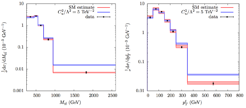
The most obvious place to look for the effects of higher-dimensional terms is through the enhancement (or reduction, in the case of destructive interference) of total cross-sections. Important differences between SM and dimension-six terms are lost in this approach, however, since operators can cause deviations in the shape of distributions without substantially impacting event yields. This is highlighted in Figure 3, where we plot our NLO SM estimate for two top pair distributions, vs. one with a large interference term. Both are consistent with the data in the threshold region, which dominates the cross-section, but clear discrimination between SM and dimension-six effects is visible in the high-mass region, which simply originates from the scaling of dimension-six operator effects as $s/\Lambda^{2}$ .

Figure 3: Parton level differential distributions in top pair production, considering SM only (red) and the effects of the four-quark operator $O^{2}_{u}$, showing the enhancement in the tails of the distributions. Data taken from Ref. [83].

Limits on these operators can be obtained in two ways; by setting all other operators to zero, and by marginalising over the other parameters in a global fit. In Figure 4 we plot the allowed 68%, 95% and 99% confidence intervals for various pairs of operators, with all others set to zero, showing correlations between some coefficients. Most of these operators appear uncorrelated, though there is a strong correlation between $C^{1}_{u}$ and $C^{1}_{d}$, due to a relative sign between their interference terms. Given the lack of reported deviations in top quark measurements, it is perhaps unsurprising to see that all Wilson coefficients are consistent with zero within the 95% confidence intervals, and that the SM hypothesis is an excellent description of the data. In Figure 5, the stronger joint constraints on $C_{G}$ vs $C^{1}_{u}$ obtained from including differential measurements make manifest the importance of utilizing all available cross-section information.

Figure 4: 68%, 95% and 99% confidence intervals for selected combinations of operators contributing to top pair production, with all remaining operators set to zero. The star marks the best fit point, indicating good agreement with the Standard Model. Here $\bar{C}_{i}=C_{i}v^{2}/\Lambda^{2}$.

Figure 5: Left: 68%, 95% and 99% confidence intervals on the operators $C_{G}$ vs. $C^{1}_{u}$ , considering differential and total cross-sections (contours, red star), and total cross-sections only (lines, white star). Right: Limits on $C^{33}_{uG}$ vs. $C^{1}_{u}$, considering both Tevatron and LHC data (contours) and Tevatron data only (lines).

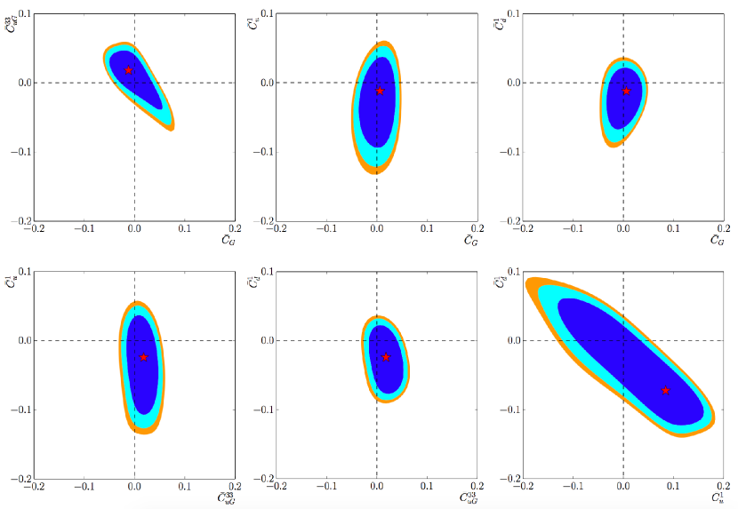
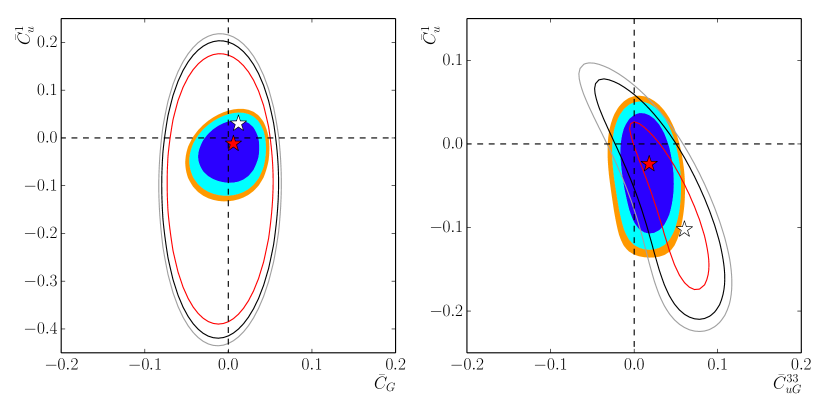
It is also interesting to note the relative pull of measurements from the LHC and Tevatron, as illustrated in Figure 5. It is interesting to see that although Tevatron data are naively more sensitive to four-quark operators, after the LHC Run I and early into Run II, the LHC data size and probed energy transfers lead to comparably stronger constraints. In our fit this is highlighted by the simple fact that LHC data comprise more than 80% of the bins in our fit, so have a much larger pull. This stresses the importance of collecting large statistics as well as using sensitive discriminating observables.

4.2 Single top production

The next most abundant source of top quark data is from single top production. In our fit we consider production in the $t$ and $s$ channels, and omit $Wt$-associated production. Though measurements of the latter process have been published, they are not suitable for inclusion in a fit involving parton level theory predictions. As is well-known, $Wt$ production interferes with top pair production at NLO and beyond in a five-flavour scheme [126, 127, 128], or at LO in a four-flavour one. Its separation from top pair production is then a delicate issue, discussed in detail in Refs. [129, 130, 131, 132]. We thus choose to postpone the inclusion of $Wt$ production to a future study, going beyond parton level. The operators that could lead to deviations from SM predictions are shown below

$$\begin{split}\mathcal{L}_{D6}&\supset\frac{C_{uW}}{\Lambda^{2}}(\bar{q}\sigma^{\mu\nu}\tau^{I}u)\,\tilde{\varphi}\,W_{\mu\nu}^{I}+\frac{C^{(3)}_{\varphi q}}{\Lambda^{2}}i(\varphi^{\dagger}\overleftrightarrow{D}^{I}_{\mu}\varphi)(\bar{q}\gamma^{\mu}\tau^{I}q)\\ &+\frac{C_{\varphi ud}}{\Lambda^{2}}(\varphi^{\dagger}\overleftrightarrow{D}_{\mu}\varphi)(\bar{u}\gamma^{\mu}d)+\frac{C_{dW}}{\Lambda^{2}}(\bar{q}\sigma^{\mu\nu}\tau^{I}d)\,\tilde{\varphi}\,W_{\mu\nu}^{I}\\ &+\frac{C^{(3)}_{qq}}{\Lambda^{2}}(\bar{q}\gamma_{\mu}\tau^{I}q)(\bar{q}\gamma^{\mu}\tau^{I}q)+\frac{C^{(1)}_{qq}}{\Lambda^{2}}(\bar{q}\gamma_{\mu}q)(\bar{q}\gamma^{\mu}q)+\frac{C^{(1)}_{qu}}{\Lambda^{2}}(\bar{q}\gamma_{\mu}q)(\bar{u}\gamma^{\mu}u)\,.\end{split}$$ (10)

As in top pair production there are several simplifications which reduce this operator set. The right-chiral down quark fields appearing in $O_{dW}$ and $O_{\varphi ud}$ cause these operators’ interference with the left-chiral SM weak interaction to be proportional to the relevant down-type quark mass. For example, an operator insertion of $O^{33}_{\varphi ud}$ will always contract with the SM $Wtb$ -vertex to form a term of order $m_{b}\,m_{t}\,C^{33}_{\varphi ud}/\Lambda^{2}$. Since $m_{b}$ is much less than both $\hat{s}$ and the other dimensionful parameters that appear, $v$ and $m_{t}$, we may choose to neglect these operators. By the same rationale we neglect $O^{(1)}_{qu}$ as its contribution to observables is $\mathcal{O}(m_{u})$. We have further checked numerically that the contribution of these operators is practically negligible. Finally, all contributing four-fermion partonic subprocesses depend only on the linear combination of Wilson Coefficients:

$$\begin{split}C_{t}=&~{}C^{(3){1331}}_{qq}+\tfrac{1}{6}(C^{(1){1331}}_{qq}-C^{(3)1331}_{qq}).\end{split}$$ (11)

Single top production can thus be characterised by the three dimension-six operators $O_{uW}$, $O^{(3)}_{\varphi q}$ and $O_{t}$.

As noted in the introduction, several model-independent studies have noted the potential for uncovering new physics in single top production, though these have typically been expressed in terms of anomalous couplings, via the Lagrangian

$$\mathcal{L}_{Wtb}=\frac{g}{\sqrt{2}}\bar{b}\gamma^{\mu}(V_{L}P_{L}+V_{R}P_{R})tW^{-}_{\mu}+\frac{g}{\sqrt{2}}\bar{b}\frac{i\sigma^{\mu\nu}q_{\nu}}{M_{W}}(g_{L}P_{L}+g_{R}P_{R})tW^{-}_{\mu}+h.c.\,$$ (12)

where $q=p_{t}-p_{b}$. There is a one-to-one mapping between this Lagrangian and those dimension-six operators that modify the $Wtb$ vertex:

$$V_{L} \to V_{tb}+C^{(3)}_{\varphi q}v^{2}/\Lambda^{2} V_{R} \to\frac{1}{2}C_{\varphi ud}v^{2}/\Lambda^{2}$$

$$g_{L} \to\sqrt{2}C_{uW}v^{2}/\Lambda^{2} g_{R} \to\sqrt{2}C_{dW}v^{2}/\Lambda^{2}$$ (13)

What, then, is the advantage of using higher-dimensional operators when anomalous couplings capture most of the same physics? The advantages are manifold. Firstly, the power-counting arguments of the previous paragraph that allowed us to reject the operators $O_{dW}$, $O_{\varphi ud}$ at order $\Lambda^{-2}$ would not be clear in an anomalous coupling framework. In addition, the four-quark operator $O^{(3)}_{qq}$ in eq. (10) can have a substantial effect on single-top production, but this can only be captured by an EFT approach. For a detailed comparison of these approaches, see e.g. Ref. [133]. The 95% confidence limits on these operators from single top production are shown in Fig. (6), along with those operators previously discussed in top pair production.

Figure 6: Left: Individual (red) and marginalised (blue) 95% confidence intervals on dimension-six operators from top pair production and single top production (bottom three). Right: Marginalised 95 % bounds considering all data from LHC and Tevatron (green) vs Tevatron only (purple).

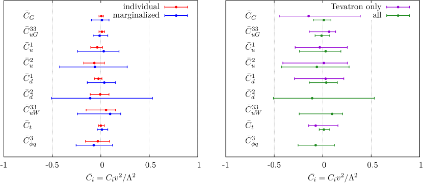
Let us compare these results to our findings of Section 4.1. The bounds on operators from top pair production are typically stronger. The so-called chromomagnetic moment operator $O_{uG}$ is also tightly constrained, owing to its appearance in both the $q\bar{q}$ and $gg$ channels, i.e. it is sensitive to both Tevatron and LHC measurements. For the four-quark operators, the stronger bounds are typically on the $C^{1}_{i}$-type. This originates from the more pronounced effect on kinematic distributions that they have. The phenomenology of the $C^{2}_{i}$-type operators is SM-like, and their effect becomes only visible in the tails of distributions.

The much wider marginalised bounds on these two operators stems from the relative sign between their interference term and those of the other operators, which results in cancellations in the total cross-section that significantly widen the allowed ranges of $C_{i}$. With the exception of $C_{t}$, which strongly modifies the single top production cross-section, the individual bounds on the operator coefficients from single top production are typically weaker. This originates from the larger experimental uncertainties on single top production, that stem from the multitude of different backgrounds that contaminate this process, particularly top pair production. For the Tevatron datasets this is particularly telling: the few measurements that have been made, with no differential distributions, combined with the large error bars on the available data, mean that two of the three operators are not constrained at dimension-six. Still, as before, excellent agreement with the SM is observed.

In addition to single-top production, the operator $O_{uW}$ may be constrained by distributions relating to the kinematics of the top quark decay. The matrix element for hadronic top quark decay $t\to Wb\to bqq^{\prime}$, for instance, is equivalent to that for $t$-channel single top production via crossing symmetry, so decay observables provide complementary information on this operator. We will discuss the bounds obtainable from decay observables in Section 4.4.

4.3 Associated production

In addition to top pair and single top production, first measurements have been reported [98, 99, 100] of top pair production in association with a photon and with a $Z$ boson ($t\bar{t}\gamma$ and $t\bar{t}Z$). The cross-section for these processes are considerably smaller, and statistical uncertainties currently dominate the quoted measurements. Still, they are of interest because they are sensitive to a new set of operators not previously accessible, corresponding to enhanced top-gauge couplings which are ubiquitous in simple $W^{\prime}$ and $Z$ models, and which allow contact to be made with electroweak observables. The operator set for $t\bar{t}Z$, for instance, contains the 6 top pair operators in eq. (8), plus the following

$$\begin{split}\mathcal{L}_{D6}&\supset\frac{C_{uW}}{\Lambda^{2}}(\bar{q}\sigma^{\mu\nu}\tau^{I}u)\,\tilde{\varphi}\,W_{\mu\nu}^{I}+\frac{C_{uB}}{\Lambda^{2}}(\bar{q}\sigma^{\mu\nu}u)\,\tilde{\varphi}\,B_{\mu\nu}+\frac{C^{(3)}_{\varphi q}}{\Lambda^{2}}i(\varphi^{\dagger}\overleftrightarrow{D}^{I}_{\mu}\varphi)(\bar{q}\gamma^{\mu}\tau^{I}q)\\ &+\frac{C^{(1)}_{\varphi q}}{\Lambda^{2}}i(\varphi^{\dagger}\overleftrightarrow{D}_{\mu}\varphi)(\bar{q}\gamma^{\mu}q)+\frac{C_{\varphi u}}{\Lambda^{2}}(\varphi^{\dagger}i\overleftrightarrow{D}_{\mu}\varphi)(\bar{u}\gamma^{\mu}u)\,.\end{split}$$ (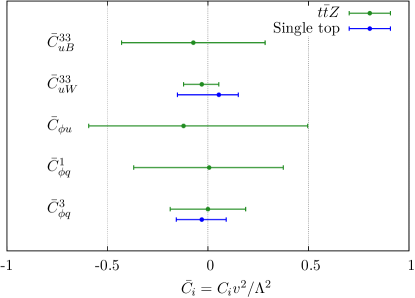14)

There is therefore overlap between the operators contributing to associated production, and those contributing to both top pair and single top. In principle, one should include all observables in a global fit, fitting all coefficients simultaneously. However, the low number of individual $t\bar{t}V$ measurements, coupled with their relatively large uncertainties, means that they do not have much effect on such a fit. Instead, we choose to present individual constraints on the operators from associated production alone, comparing these with top pair and single top in what follows. For the former, we find that the constraints on the operators of eq. (14) obtained from $t\bar{t}\gamma$ and $t\bar{t}Z$ measurements are much weaker than those obtained from top pair production, therefore we do not show them here. The constraints on the new operators of eq. (14) are displayed in Figure 7. It is interesting to note that the constraints from associated production measurements are comparable with those from single top production, despite the relative paucity of the former.

Figure 7: Individual 95% confidence intervals for the operators of 14 from $t\bar{t}\gamma$ and $t\bar{t}Z$ production (green) and in the two cases where there is overlap, from single top measurements (blue).

4.4 Decay observables

This completes the list of independent dimension-six operators that affect top quark production cross-sections. However, dimension-six operators may also contribute (at interference level) to observables relating to top quark decay. Top quarks decay almost 100% of the time to a $W$ and $b$ quark. The fraction of these events which decay to $W$-bosons with a given helicity: left-handed, right-handed or zero-helicity, can be expressed in terms of helicity fractions, which for leading order with a finite $b$-quark mass are

$$\begin{split}F_{0}&=\frac{(1-y^{2})^{2}-x^{2}(1+y^{2})}{(1-y^{2})^{2}+x^{2}(1-2x^{2}+y^{2})}\\ F_{L}&=\frac{x^{2}(1-x^{2}+y^{2})+\sqrt{\lambda}}{(1-y^{2})^{2}+x^{2}(1-2x^{2}+y^{2})}\\ F_{R}&=\frac{x^{2}(1-x^{2}+y^{2})-\sqrt{\lambda}}{(1-y^{2})^{2}+x^{2}(1-2x^{2}+y^{2})}\end{split}$$ (15)

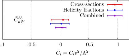
where $x=M_{W}/m_{t}$, $y=m_{b}/m_{t}$ and $\lambda=1+x^{4}+y^{4}-2x^{2}y^{2}-2x^{2}-2y^{2}$. As noted in Ref. [46], measurements of these fractions can be translated into bounds on the operator $O_{uW}$. (The operator $O^{(3)}_{\varphi q}$ cannot be accessed in this way, since its only effect is to rescale the $Wtb$ vertex $V^{2}_{tb}\to V_{tb}\left(V_{tb}+v^{2}C^{(3)}_{\varphi q}/\Lambda^{2}\right)$, therefore it has no effect on event kinematics.) The desirable feature of these quantities is that they are relatively stable against higher order corrections, so the associated scale uncertainties are small. The Standard Model NNLO estimates for these are: $\{F_{0},F_{L},F_{R}\}=\{0.687\pm 0.005,0.311\pm 0.005,0.0017\pm 0.0001\}$ [134], i.e. the uncertainties are at the per mille level. It is interesting to ask whether the bound obtained on $O_{uW}$ in this way is stronger than that obtained from cross-section measurements. In Figure 8 we show the constraints obtained in each way. Although they are in excellent agreement with each other, cross-section information gives a slightly stronger bound, mainly due to the larger amount of data available, but also due to the large experimental uncertainties on $F_{i}$. Still, these measurements provide complementary information on the operator $O_{uW}$, and combining both results in a stronger constraint than either alone, as expected.

Figure 8: 95% bounds on the operator $O_{uW}$ obtained from data on top quark helicity fractions (blue) vs. single top production cross-sections (red), and both sets of measurements combined (purple).

4.5 Charge asymmetries

Asymmetries in the production of top quark pairs have received a lot of attention in recent years, particularly due to an apparent discrepancy between the Standard Model prediction for the so-called ‘forward-backward’ asymmetry $A_{\mathrm{FB}}$ in top pair production

$$A_{\mathrm{FB}}=\frac{N(\Delta y>0)-N(\Delta y<0)}{N(\Delta y>0)+N(\Delta y<0)}$$ (16)

where $\Delta y=y_{t}-y_{\bar{t}}$, and a measurement by CDF [135]. This discrepancy was most pronounced in the high invariant mass region, pointing to potential TeV-scale physics at play. However, recent work has cast doubts on its significance for two reasons: Firstly, an updated analysis with higher statistics [90] has slightly lowered the excess. Secondly, a full NNLO QCD calculation [136] of $A_{\mathrm{FB}}$ showed that, along with NLO QCD + electroweak calculations [137, 138, 139] the radiative corrections to $A_{\mathrm{FB}}$ are large. The current measurements are now consistent with the Standard Model within 2$\sigma$. Moreover, the D${\not{0}}$ experiment reports [91] a high-invariant mass measurement lower than the SM prediction. From a new physics perspective, it is difficult to accommodate all of this information in a simple, uncontrived model without tension.

Figure 9: Results of a 1000 point parameter space scan over -10 TeV ${}^{-2}<C^{1,2}_{u,d}/\Lambda^{2}<$ 10 $TeV^{-2}$ overlaid with the most up to date measurements of $A_{\mathrm{FB}}$ and $A_{\mathrm{C}}$, showing clearly the correlation between them.

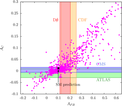
Still, in an effective field theory approach, deviations from the Standard Model prediction of $A_{\mathrm{FB}}$ take a very simple form. A non-zero asymmetry arises from the difference of four-quark operators:

$$A_{\mathrm{FB}}=(C^{1}_{u}-C^{2}_{u}+C^{1}_{d}-C^{2}_{d})\frac{3\hat{s}\beta}{4g_{s}^{2}\Lambda^{2}(3-\beta^{2})},$$ (17)

where $\beta=\sqrt{1-s/4m_{t}^{2}}$ is the velocity of the $t\bar{t}$ system. Combining this inclusive measurement with differential measurements such as $dA_{\mathrm{FB}}/dM_{t\bar{t}}$ allows simultaneous bounds to be extracted on all four of these operators. Therefore it is instructive to compare the bounds obtained on $C^{1,2}_{u,d}$ from charge asymmetries to those obtained from $t\bar{t}$ cross-sections. Again it is possible to (indirectly) investigate the complementarity between Tevatron and LHC constraints. Though the charge symmetric initial state of the LHC does not define a ‘forward-backward’ direction, a related charge asymmetry can be defined as:

$$A_{C}=\frac{N(\Delta|y|>0)-N(\Delta|y|<0)}{N(\Delta|y|>0)+N(\Delta|y|<0)}$$ (18)

making use of the fact that tops tend to be produced at larger rapidities than antitops. This asymmetry is diluted with respect to $A_{\mathrm{FB}}$, however. The most up-to-date SM prediction is $A_{C}=0.0123\pm 0.005$ [139] for $\sqrt{s}=$ 7 TeV. The experimental status of these measurements is illustrated in Figure 9. The inclusive measurements of $A_{\mathrm{FB}}$ are consistent with the SM expectation, as are those of $A_{\mathrm{C}}$. The latter, owing to large statistical errors, are also consistent with zero, however, so this result is not particularly conclusive. Since these are different measurements, it is also possible to modify one without significantly impacting the other. Clearly they are correlated, as evidenced in Figure 9, where the most up to date measurements of $A_{\mathrm{FB}}$ and $A_{\mathrm{C}}$ are shown along with the results of a 1000 point parameter space scan over the four-quark operators. This highlights the correlation between the two observables: non-resonant new physics which causes a large $A_{\mathrm{FB}}$ will also cause a large $A_{\mathrm{C}}$, provided it generates a dimension-six operator at low energies.

We have used both inclusive measurements of the charge asymmetries $A_{\mathrm{C}}$ and $A_{\mathrm{FB}}$, and measurements as a function of the top pair invariant mass $M_{t\bar{t}}$ and rapidity difference $|y_{t\bar{t}}|$. In addition, ATLAS has published measurements of $A_{\mathrm{C}}$ with a longitudinal ‘boost’ of the $t\bar{t}$ system: $\beta=(|p^{z}_{t}+p^{z}_{\bar{t}})|/(E_{t}+E_{\bar{t}})>0.6$, which may enhance sensitivity to new physics contributions to $A_{\mathrm{C}}$, depending on the model [143].

Since $A_{\mathrm{FB}}=0$ at leading-order in the SM, it is not possible to define a $K$-factor in the usual sense. Instead we take higher-order QCD effects into account by adding the NNLO QCD prediction to the dimension-six terms. In the case of $A_{\mathrm{C}}$, we normalise the small (but non-zero) LO QCD piece, to the NLO prediction, which has been calculated with a Monte Carlo and cross-checked with a dedicated NLO calculation [139].

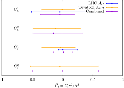
The above asymmetries have been included in the global fit results presented in Figure 12. However, it is also interesting to see what constraints are obtained on the operators from asymmetry data alone. To this end, the 95% confidence intervals on the coefficients of the operators $O^{1,2}_{u,d}$ from purely charge asymmetry data are shown in Figure 10. Unsurprisingly, the bounds are much weaker than for cross-section measurements, with the $O^{2}_{i}$-type operators unconstrained by LHC data alone. Despite the small discrepancy between the measured $A_{\mathrm{FB}}$ and its SM value, this does not translate into a non-zero Wilson coefficient; as before, all operators are zero within the 95% confidence intervals.

At 13 TeV, the asymmetry $A_{\mathrm{C}}$ will be diluted even further, due to the increased dominance of the $gg\to t\bar{t}$ channel, for which $A_{C}=0$. It is therefore possible that charge asymmetry measurements (unlike cross-sections) will not further tighten the bounds on these operators during LHC Run II.

Figure 10: Marginalised 95% confidence intervals on top pair four quark operators from charge asymmetries at the LHC and Tevatron.

4.6 Contribution of individual datasets

As well as the constraints presented in Figure 12, it is also instructive to examine the quality of fit for different datasets. We quantify this by calculating the $\chi^{2}$ per bin between the data and the global best fit point, as shown in Figure 11.

Figure 11: $\chi^{2}$ per bin between measurement and the interpolated best fit point, for measurements considered in this fit. Colours: Green: ATLAS 7 TeV, Magenta: ATLAS 8 TeV, Blue: CMS 7 TeV, Turquoise: CMS 8 TeV, Red: D${\not{0}}$, Orange: CDF, Purple: CMS 13 TeV.

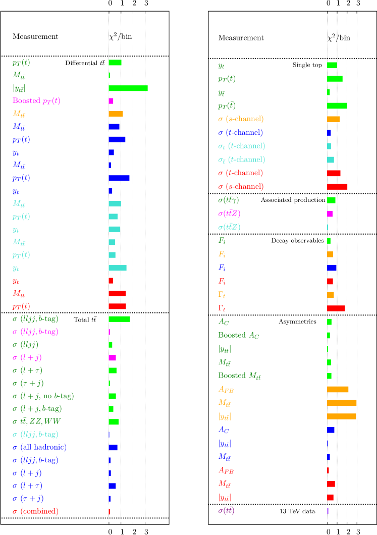
Overall, excellent agreement is seen across the board, with no measurement in obvious tension with any other. The largest single contributors to the $\chi^{2}$ come from the rapidity distributions in top pair production. It has been known for some time that these are quite poorly modelled with Monte Carlo generators, especially in the boosted regime. It is quite likely that this discrepancy stems from the QCD modelling of the event kinematics, rather than potential new physics. Moreover, in a fit with this many measurements, discrepancies of this magnitude are to be expected on purely statistical grounds.

At the level of total cross-sections, the vanishingly small contributions to the $\chi^{2}$ stem from two factors: the $\mathcal{O}(10\%)$ measurement uncertainties, which are even larger in hadronic channels, and the large scale uncertainties from the large kinematic range that is integrated over to obtain the total rate. Single top production measurements are also in good agreement with the SM. The associated production processes $tt\gamma$ and $ttZ$, along with the charge asymmetry measurements from the LHC, have a very small impact on the fit, owing to the large statistical uncertainties on the current measurements. For the former, this situation will improve in Run II, for the latter the problem will be worse. The forward-backward asymmetry measurements from CDF remain the most discrepant dataset used in the fit.

5 Constraining UV models

As an illustration of the wide-ranging applicability of EFT techniques, we conclude by matching our effective operator constraints to the low-energy regime of some specific UV models. These models serve purely illustrative purposes.

5.1 Axigluon searches

Considering top pair production, one can imagine the four operators of eq. (9) as being generated by integrating out a heavy $s$-channel resonance which interferes with the QCD $q\bar{q}\to t\bar{t}$ amplitude. One particle that could generate such an interference is the so-called axigluon. These originate from models with an extended strong sector with gauge group $SU(3)_{c1}\times SU(3)_{c2}$ which is spontaneously broken to the diagonal subgroup $SU(3)_{c}$ of QCD. In the most minimal scenario, this breaking can be described by a non-linear sigma model

$$\mathcal{L}=-\frac{1}{4}G_{1\mu\nu}G_{1}^{\mu\nu}-\frac{1}{4}G_{2\mu\nu}G_{2}^{\mu\nu}+\frac{f^{2}}{4}\text{Tr}D_{\mu}\Sigma D^{\mu}\Sigma^{\dagger}\hskip 10.0pt,\hskip 10.0pt\Sigma=\exp\left(\frac{2i\pi^{a}t^{a}}{f}\right)\hskip 10.0pt,\hskip 10.0pta=1,...,8.$$ (19)

Here $\pi^{a}$ represent the Goldstone bosons which form the longitudinal degrees of freedom of the colorons, giving them mass, $t^{a}$ are the Gell-Mann matrices, and $f$ is the symmetry breaking scale. The nonlinear sigma fields transform in the bifundamental representation of $SU(3)_{c1}\times SU(3)_{c2}$:

$$\Sigma\to U_{L}\Sigma U^{\dagger}_{R}\hskip 10.0pt,\hskip 10.0ptU_{L}=\exp\left(\frac{i\pi^{a}\alpha_{L}^{a}}{f}\right)\hskip 10.0pt,\hskip 10.0ptU_{R}=\exp\left(\frac{i\pi^{a}\alpha_{R}^{a}}{f}\right)$$ (20)

The physical fields are obtained by rotating the gauge fields $G_{1}$ and $G_{2}$ to the mass eigenstate basis

$$\left(\begin{array}[]{c}G^{a}_{1\mu}\\ G^{a}_{2\mu}\end{array}\right)=\left(\begin{array}[]{c c}\cos\theta_{c}&-\sin\theta_{c}\\ \sin\theta_{c}&\cos\theta_{c}\end{array}\right)\left(\begin{array}[]{c}G^{a}_{\mu}\\ C^{a}_{\mu}\end{array}\right)$$ (21)

where the mixing angle $\theta_{c}$ is defined by

$$\sin\theta_{c}=\frac{g_{s1}}{\sqrt{g^{2}_{s1}+g^{2}_{s2}}}$$ (22)

The case of an axigluon corresponds to maximal mixing $\theta=\pi/4$, i.e. $g^{2}_{s1}=g^{2}_{s2}=g^{2}_{s}/2$. Taking the leading-order interference with the SM amplitude for $q\bar{q}\to t\bar{t}$, in the limit $s<<M_{A}^{2}$, we find that the axigluon induces the dimension-six operators

$$\frac{C^{1}_{u}}{\Lambda^{2}}=\frac{g^{2}_{s}}{M_{A}^{2}},\hskip 10.0pt\hskip 10.0pt\frac{C^{1}_{d}}{\Lambda^{2}}=\frac{5g^{2}_{s}}{4M_{A}^{2}},\hskip 10.0pt\hskip 10.0pt\frac{C^{2}_{u}}{\Lambda^{2}}=\frac{C^{2}_{d}}{\Lambda^{2}}=\frac{2g^{2}_{s}}{M_{A}^{2}}$$ (23)

Substituting the marginalised constraints on the 4-quark operators, we find this translates into a lower bound on an axigluon mass. $M_{A}\gtrsim 1.4$ TeV at the 95% confidence level. Since this mass range coincides with the overflow bin of figure 3, this bound creates some tension with the validity of the EFT approach in the presence of resonances in the $t\bar{t}$ spectrum (for a general discussion see Ref. [114, 144, 145]); at this stage in the LHC programme indirect searches are not sensitive enough to compete with dedicated searches.

5.2 $W^{\prime}$ searches

Turning our attention to single top production, we consider the example of the operator $O^{(3)}_{qq}$ being generated by a heavy charged vector resonance ($W^{\prime}$) which interferes with the SM amplitude for $s$-channel single top production: $u\bar{d}\to W\to t\bar{b}$. The most general Lagrangian for such a particle (allowing for left and right chiral couplings) is (see e.g. Ref. [146].)

$$\mathcal{L}=\frac{1}{2\sqrt{2}}V_{ij}g_{W^{\prime}}\bar{q}_{i}\gamma_{\mu}(f^{R}_{ij}(1+\gamma^{5})+f^{L}_{ij}(1-\gamma^{5}))W^{\mu}q_{j}+h.c.$$ (24)

We take the generic coupling $g_{W^{\prime}}=g_{SM}$. Since we are considering the interference term only, which must have the same $(V-A)$ structure as the SM, we can set $f^{R}=0$. Considering the tree-level interference term for between the diagrams for $u\bar{d}\to W^{\prime},W^{\prime}\to t\bar{b}$, and taking the limit $s\ll M_{W}^{\prime 2}$ (we also work in the narrow-width approximation $\Gamma_{W},\Gamma_{W^{\prime}}\ll M_{W},M_{W^{\prime}}$), we find

$$\frac{C^{3,1133}_{qq}}{\Lambda^{2}}=\frac{g^{2}}{4M^{2}_{W^{\prime}}}$$ (25)

which, using our global constraint on $O_{t}$, translates into a bound $M_{W^{\prime}}\gtrsim 1.2$ TeV.

These bounds are consistent with, but much weaker than, constraints from direct searches for dijet resonances from ATLAS [147, 148] and CMS [149], which report lower bounds of $\{M_{A},M_{W^{\prime}}\}>\{2.72,3.32\}$ TeV and $\{M_{A},M_{W^{\prime}}\}>\{2.2,3.6\}$ TeV respectively. It is unsurprising that these dedicated analyses obtain stronger limits, given the generality of this fit. Again this energy range is resolved in our fit thus in principle invalidating the EFT approach to obtain eq. (25). Nonetheless, these bounds provide an interesting comparison of our numerical results, whilst emphasising that for model-specific examples, direct searches for high-mass resonances provide stronger limits than general global fits.

6 Conclusion

In this paper, we have performed an up-to-date global fit of top quark effective field theory to experimental data, including all constrainable operators at dimension six. For the operators, we use the ‘Warsaw basis’ of Ref. [54], which has also been widely used in the context of Higgs and precision electroweak physics. We use data from the Tevatron and LHC experiments, including LHC Run II data, up to a centre of mass energy of 13 TeV. Furthermore, we include fully inclusive cross-section measurements, as well as kinematic distributions involving both the production and decay of the top quark. Counting each bin independently, the total number of observables entering our fit is 227, with a total of 13 contributing operators. Constraining the coefficients of these operators is then a formidable computational task. To this end we use the parametrisation methods in the Professor framework, first developed in the context of Monte Carlo generator tuning [53], and discussed here in Section 3.

Figure 12: 95% confidence intervals for the dimension-six operators that we consider here, with all remaining operators set to zero (red) and marginalised over (blue). In cases where there are constraints on the same operator from different classes of measurement, the strongest limits are shown here. The lack of marginalised constraints for the final three operators is discussed in Section 4.3.

Coefficient	Individual constraint	Marginalised constraint
$C_{G}v^{2}/\Lambda^{2}$	(—0.018, 0.027)	(—0.097, 0.085)
$C^{33}_{uG}v^{2}/\Lambda^{2}$	(—0.018, 0.039)	(—0.079, 0.073)
$C^{1}_{u}v^{2}/\Lambda^{2}$	(—0.103, 0.018)	(—0.236, 0.188)
$C^{2}_{u}v^{2}/\Lambda^{2}$	(—0.175, 0.036)	(—0.424, 0.272)
$C^{1}_{d}v^{2}/\Lambda^{2}$	(—0.067, 0.012)	(—0.139, 0.151)
$C^{2}_{d}v^{2}/\Lambda^{2}$	(—0.109, 0.085)	(—0.508, 0.533)
$C^{33}_{uW}v^{2}/\Lambda^{2}$	(—0.079, 0.109)	(—0.242, 0.206)
$C_{t}v^{2}/\Lambda^{2}$	(—0.024, 0.036)	(—0.036, 0.073)
$C^{3}_{\varphi q}v^{2}/\Lambda^{2}$	(—0.157, 0.091)	(—0.254, 0.121)
$C^{33}_{uB}v^{2}/\Lambda^{2}$	(—0.430, 0.284)	(—, —)
$C_{\varphi u}v^{2}/\Lambda^{2}$	(—0.593, 0.496)	(—, —)
$C^{1}_{\varphi q}v^{2}/\Lambda^{2}$	(—0.369, 0.375)	(—, —)

Table 2: Numerical values of the individual and marginalised 95% confidence intervals on the operators presented here.

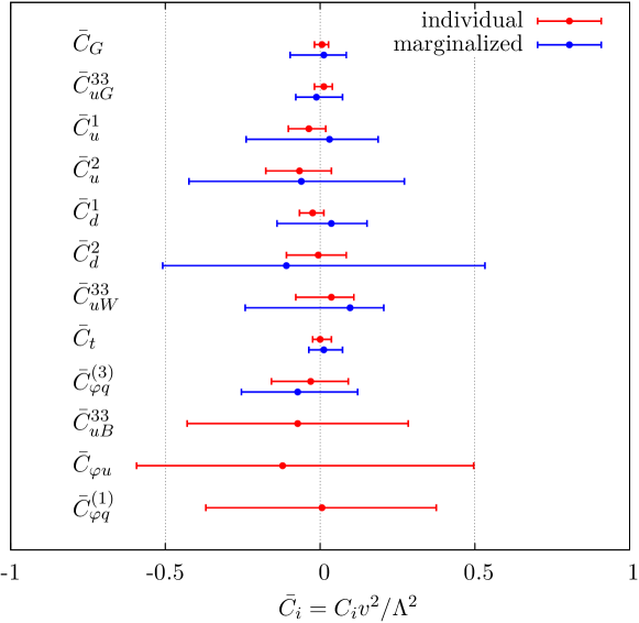
We perform a $\chi^{2}$ fit of theory to data, including appropriate correlation matrices where these have been provided by the experiments. We obtain bounds on the Wilson coefficients of various operators contributing to top quark production and decay, summarised in Figure 12, in two cases: (i) when all other coefficients are set to zero; (ii) when all other operators coefficients are marginalised over. The numerical values of these constraints are also shown in Table 2.

Our stronger constraints are on operators involving the gluon, as expected given the dominance of gluon fusion in top pair production at the LHC (for which there is more precise data). Four fermion operators are constrained well in general, with weaker constraints coming from processes whose experimental uncertainties remain statistically dominated (e.g. $t\bar{t}V$ production). We have quantified the interplay between the Tevatron and LHC datasets, as well as that between different measurement types (e.g. top pair, single top).

Our results currently agree well with the SM only, which is perhaps to be expected given the lack of reported deviations in previous studies. However, the fact that this agreement is obtained, in a wide global fit, is itself testament to the consistency of different top quark measurements, with no obvious tension between overlapping datasets. There are a number of directions for further study. Firstly, we can improve the theory description in our fit, to include higher order QCD corrections in a more rigorous way, as well as moving away from parton level observables. Secondly, new data from LHC Run II is continuously appearing, and can be implemented in our fit as soon as it is available. The era of performing large global fits to widely different data in the top quark sector is now upon us, and our work on this area is ongoing.

References

- [1] T. Appelquist and J. Carazzone, “Infrared Singularities and Massive Fields,” Phys. Rev. D11 (1975) 2856.
- [2] K. G. Wilson, “The renormalization group and critical phenomena,” Rev. Mod. Phys. 55 (1983) 583–600.
- [3] S. F. King, M. Muhlleitner, R. Nevzorov, and K. Walz, “Natural NMSSM Higgs Bosons,” Nucl. Phys. B870 (2013) 323–352, arXiv:1211.5074 [hep-ph].
- [4] W. Buchmuller and D. Wyler, “Effective Lagrangian Analysis of New Interactions and Flavor Conservation,” Nucl. Phys. B268 (1986) 621–653.
- [5] K. Hagiwara, R. Peccei, D. Zeppenfeld, and K. Hikasa, “Probing the Weak Boson Sector in ,” Nucl.Phys. B282 (1987) 253.
- [6] C. J. C. Burges and H. J. Schnitzer, “Virtual Effects of Excited Quarks as Probes of a Possible New Hadronic Mass Scale,” Nucl. Phys. B228 (1983) 464.
- [7] C. N. Leung, S. T. Love, and S. Rao, “Low-Energy Manifestations of a New Interaction Scale: Operator Analysis,” Z. Phys. C31 (1986) 433.
- [8] A. Azatov, R. Contino, and J. Galloway, “Model-Independent Bounds on a Light Higgs,” JHEP 04 (2012) 127, arXiv:1202.3415 [hep-ph]. [Erratum: JHEP04,140(2013)].
- [9] J. R. Espinosa, C. Grojean, M. Muhlleitner, and M. Trott, “First Glimpses at Higgs’ face,” JHEP 12 (2012) 045, arXiv:1207.1717 [hep-ph].
- [10] T. Plehn and M. Rauch, “Higgs Couplings after the Discovery,” Europhys. Lett. 100 (2012) 11002, arXiv:1207.6108 [hep-ph].
- [11] D. Carmi, A. Falkowski, E. Kuflik, T. Volansky, and J. Zupan, “Higgs After the Discovery: A Status Report,” JHEP 10 (2012) 196, arXiv:1207.1718 [hep-ph].
- [12] M. E. Peskin, “Comparison of LHC and ILC Capabilities for Higgs Boson Coupling Measurements,” arXiv:1207.2516 [hep-ph].
- [13] B. Dumont, S. Fichet, and G. von Gersdorff, “A Bayesian view of the Higgs sector with higher dimensional operators,” JHEP 07 (2013) 065, arXiv:1304.3369 [hep-ph].
- [14] A. Djouadi and G. Moreau, “The couplings of the Higgs boson and its CP properties from fits of the signal strengths and their ratios at the 7+8 TeV LHC,” Eur. Phys. J. C73 no. 9, (2013) 2512, arXiv:1303.6591 [hep-ph].
- [15] D. Lopez-Val, T. Plehn, and M. Rauch, “Measuring extended Higgs sectors as a consistent free couplings model,” JHEP 10 (2013) 134, arXiv:1308.1979 [hep-ph].
- [16] C. Englert, A. Freitas, M. M. Muehlleitner, T. Plehn, M. Rauch, M. Spira, and K. Walz, “Precision Measurements of Higgs Couplings: Implications for New Physics Scales,” J. Phys. G41 (2014) 113001, arXiv:1403.7191 [hep-ph].
- [17] J. Ellis, V. Sanz, and T. You, “Complete Higgs Sector Constraints on Dimension-6 Operators,” JHEP 07 (2014) 036, arXiv:1404.3667 [hep-ph].
- [18] J. Ellis, V. Sanz, and T. You, “The Effective Standard Model after LHC Run I,” JHEP 03 (2015) 157, arXiv:1410.7703 [hep-ph].
- [19] A. Falkowski and F. Riva, “Model-independent precision constraints on dimension-6 operators,” JHEP 02 (2015) 039, arXiv:1411.0669 [hep-ph].
- [20] T. Corbett, O. J. P. Eboli, D. Goncalves, J. Gonzalez-Fraile, T. Plehn, and M. Rauch, “The Higgs Legacy of the LHC Run I,” JHEP 08 (2015) 156, arXiv:1505.05516 [hep-ph].
- [21] G. Buchalla, O. Cata, A. Celis, and C. Krause, “Fitting Higgs Data with Nonlinear Effective Theory,” arXiv:1511.00988 [hep-ph].
- [22] ATLAS Collaboration, G. Aad et al., “Constraints on non-Standard Model Higgs boson interactions in an effective field theory using differential cross sections measured in the decay channel at TeV with the ATLAS detector,” arXiv:1508.02507 [hep-ex].
- [23] L. Berthier and M. Trott, “Consistent constraints on the Standard Model Effective Field Theory,” arXiv:1508.05060 [hep-ph].
- [24] A. Falkowski, M. Gonzalez-Alonso, A. Greljo, and D. Marzocca, “Global constraints on anomalous triple gauge couplings in effective field theory approach,” arXiv:1508.00581 [hep-ph].
- [25] C. Englert, R. Kogler, H. Schulz, and M. Spannowsky, “Higgs coupling measurements at the LHC,” arXiv:1511.05170 [hep-ph].
- [26] J. A. Aguilar-Saavedra, “A Minimal set of top anomalous couplings,” Nucl. Phys. B812 (2009) 181–204, arXiv:0811.3842 [hep-ph].
- [27] C. Bernardo, N. F. Castro, M. C. N. Fiolhais, H. Gonçalves, A. G. C. Guerra, et al., “Studying the vertex structure using recent LHC results,” Phys.Rev. D90 no. 11, (2014) 113007, arXiv:1408.7063 [hep-ph].
- [28] B. Grzadkowski, Z. Hioki, K. Ohkuma, and J. Wudka, “Probing anomalous top quark couplings induced by dimension-six operators at photon colliders,” Nucl. Phys. B689 (2004) 108–126, arXiv:hep-ph/0310159 [hep-ph].
- [29] D. Nomura, “Effects of Top-quark Compositeness on Higgs Boson Production at the LHC,” JHEP 02 (2010) 061, arXiv:0911.1941 [hep-ph].
- [30] Z. Hioki and K. Ohkuma, “Search for anomalous top-gluon couplings at LHC revisited,” Eur. Phys. J. C65 (2010) 127–135, arXiv:0910.3049 [hep-ph].
- [31] Z. Hioki and K. Ohkuma, “Addendum to: Search for anomalous top-gluon couplings at LHC revisited,” Eur. Phys. J. C71 (2011) 1535, arXiv:1011.2655 [hep-ph].
- [32] Z. Hioki and K. Ohkuma, “Latest constraint on nonstandard top-gluon couplings at hadron colliders and its future prospect,” Phys. Rev. D88 (2013) 017503, arXiv:1306.5387 [hep-ph].
- [33] J. A. Aguilar-Saavedra, B. Fuks, and M. L. Mangano, “Pinning down top dipole moments with ultra-boosted tops,” Phys. Rev. D91 (2015) 094021, arXiv:1412.6654 [hep-ph].
- [34] C.-R. Chen, F. Larios, and C. P. Yuan, “General analysis of single top production and helicity in top decay,” Phys. Lett. B631 (2005) 126–132, arXiv:hep-ph/0503040 [hep-ph].
- [35] J. A. Aguilar-Saavedra, “Single top quark production at LHC with anomalous Wtb couplings,” Nucl. Phys. B804 (2008) 160–192, arXiv:0803.3810 [hep-ph].
- [36] J. A. Aguilar-Saavedra and J. Bernabeu, “W polarisation beyond helicity fractions in top quark decays,” Nucl. Phys. B840 (2010) 349–378, arXiv:1005.5382 [hep-ph].
- [37] J. A. Aguilar-Saavedra, N. F. Castro, and A. Onofre, “Constraints on the Wtb vertex from early LHC data,” Phys. Rev. D83 (2011) 117301, arXiv:1105.0117 [hep-ph].
- [38] M. Fabbrichesi, M. Pinamonti, and A. Tonero, “Limits on anomalous top quark gauge couplings from Tevatron and LHC data,” Eur. Phys. J. C74 no. 12, (2014) 3193, arXiv:1406.5393 [hep-ph].
- [39] M. Fabbrichesi, M. Pinamonti, and A. Tonero, “Stringent limits on top-quark compositeness from production at the Tevatron and the LHC,” Phys. Rev. D89 no. 7, (2014) 074028, arXiv:1307.5750 [hep-ph].
- [40] Q.-H. Cao, B. Yan, J.-H. Yu, and C. Zhang, “A General Analysis of anomalous Couplings,” arXiv:1504.03785 [hep-ph].
- [41] G. A. Gonzalez-Sprinberg, R. Martinez, and J. Vidal, “Top quark tensor couplings,” JHEP 07 (2011) 094, arXiv:1105.5601 [hep-ph]. [Erratum: JHEP05,117(2013)].
- [42] S. Davidson, M. L. Mangano, S. Perries, and V. Sordini, “Lepton Flavour Violating top decays at the LHC,” Eur. Phys. J. C75 no. 9, (2015) 450, arXiv:1507.07163 [hep-ph].
- [43] S. Jung, P. Ko, Y. W. Yoon, and C. Yu, “Renormalization group-induced phenomena of top pairs from four-quark effective operators,” JHEP 08 (2014) 120, arXiv:1406.4570 [hep-ph].
- [44] Q.-H. Cao, J. Wudka, and C. P. Yuan, “Search for new physics via single top production at the LHC,” Phys. Lett. B658 (2007) 50–56, arXiv:0704.2809 [hep-ph].
- [45] C. Degrande, J.-M. Gerard, C. Grojean, F. Maltoni, and G. Servant, “Non-resonant New Physics in Top Pair Production at Hadron Colliders,” JHEP 03 (2011) 125, arXiv:1010.6304 [hep-ph].
- [46] C. Zhang and S. Willenbrock, “Effective-Field-Theory Approach to Top-Quark Production and Decay,” Phys. Rev. D83 (2011) 034006, arXiv:1008.3869 [hep-ph].
- [47] N. Greiner, S. Willenbrock, and C. Zhang, “Effective Field Theory for Nonstandard Top Quark Couplings,” Phys. Lett. B704 (2011) 218–222, arXiv:1104.3122 [hep-ph].
- [48] C. Degrande, N. Greiner, W. Kilian, O. Mattelaer, H. Mebane, T. Stelzer, S. Willenbrock, and C. Zhang, “Effective Field Theory: A Modern Approach to Anomalous Couplings,” Annals Phys. 335 (2013) 21–32, arXiv:1205.4231 [hep-ph].
- [49] J. de Blas, M. Chala, and J. Santiago, “Renormalization Group Constraints on New Top Interactions from Electroweak Precision Data,” JHEP 09 (2015) 189, arXiv:1507.00757 [hep-ph].
- [50] R. R. Aguilar, A. O. Bouzas, and F. Larios, “Limits on the anomalous couplings,” arXiv:1509.06431 [hep-ph].
- [51] G. Durieux, F. Maltoni, and C. Zhang, “Global approach to top-quark flavor-changing interactions,” Phys. Rev. D91 no. 7, (2015) 074017, arXiv:1412.7166 [hep-ph].
- [52] A. Buckley, C. Englert, J. Ferrando, D. J. Miller, L. Moore, M. Russell, and C. D. White, “Global fit of top quark effective theory to data,” Phys. Rev. D92 no. 9, (2015) 091501, arXiv:1506.08845 [hep-ph].
- [53] A. Buckley, H. Hoeth, H. Lacker, H. Schulz, and J. E. von Seggern, “Systematic event generator tuning for the LHC,” Eur.Phys.J. C65 (2010) 331–357, arXiv:0907.2973 [hep-ph].
- [54] B. Grzadkowski, M. Iskrzynski, M. Misiak, and J. Rosiek, “Dimension-Six Terms in the Standard Model Lagrangian,” JHEP 10 (2010) 085, arXiv:1008.4884 [hep-ph].
- [55] R. S. Gupta, A. Pomarol, and F. Riva, “BSM Primary Effects,” Phys. Rev. D91 no. 3, (2015) 035001, arXiv:1405.0181 [hep-ph].
- [56] G. F. Giudice, C. Grojean, A. Pomarol, and R. Rattazzi, “The Strongly-Interacting Light Higgs,” JHEP 06 (2007) 045, arXiv:hep-ph/0703164 [hep-ph].
- [57] R. Contino, M. Ghezzi, C. Grojean, M. Muhlleitner, and M. Spira, “Effective Lagrangian for a light Higgs-like scalar,” JHEP 07 (2013) 035, arXiv:1303.3876 [hep-ph].
- [58] E. Masso, “An Effective Guide to Beyond the Standard Model Physics,” JHEP 10 (2014) 128, arXiv:1406.6376 [hep-ph].
- [59] A. Pomarol, “Higgs Physics,” in 2014 European School of High-Energy Physics (ESHEP 2014) Garderen, The Netherlands, June 18-July 1, 2014. 2014. arXiv:1412.4410 [hep-ph].
- [60] A. Falkowski, B. Fuks, K. Mawatari, K. Mimasu, F. Riva, and V. sanz, “Rosetta: an operator basis translator for Standard Model effective field theory,” arXiv:1508.05895 [hep-ph].
- [61] CMS Collaboration, S. Chatrchyan et al., “Measurements of spin correlations and top-quark polarization using dilepton final states in collisions at = 7 TeV,” Phys. Rev. Lett. 112 no. 18, (2014) 182001, arXiv:1311.3924 [hep-ex].
- [62] ATLAS Collaboration, G. Aad et al., “Measurements of spin correlation in top-antitop quark events from proton-proton collisions at TeV using the ATLAS detector,” Phys. Rev. D90 no. 11, (2014) 112016, arXiv:1407.4314 [hep-ex].
- [63] ATLAS Collaboration, G. Aad et al., “Measurement of the production cross-section using events with -tagged jets in collisions at and 8 TeV with the ATLAS detector,” Eur. Phys. J. C74 no. 10, (2014) 3109, arXiv:1406.5375 [hep-ex].
- [64] ATLAS Collaboration, G. Aad et al., “Measurement of the cross section for top-quark pair production in collisions at TeV with the ATLAS detector using final states with two high-pt leptons,” JHEP 05 (2012) 059, arXiv:1202.4892 [hep-ex].
- [65] ATLAS Collaboration, G. Aad et al., “Measurement of the top quark pair cross section with ATLAS in collisions at 7 TeV using final states with an electron or a muon and a hadronically decaying lepton,” Phys. Lett. B717 (2012) 89–108, arXiv:1205.2067 [hep-ex].
- [66] ATLAS Collaboration, G. Aad et al., “Measurement of the top quark pair production cross-section with ATLAS in the single lepton channel,” Phys. Lett. B711 (2012) 244–263, arXiv:1201.1889 [hep-ex].
- [67] ATLAS Collaboration, G. Aad et al., “Measurement of the ttbar production cross section in the tau+jets channel using the ATLAS detector,” Eur. Phys. J. C73 no. 3, (2013) 2328, arXiv:1211.7205 [hep-ex].
- [68] ATLAS Collaboration, G. Aad et al., “Simultaneous measurements of the , , and production cross-sections in collisions at TeV with the ATLAS detector,” Phys. Rev. D91 no. 5, (2015) 052005, arXiv:1407.0573 [hep-ex].
- [69] ATLAS Collaboration, G. Aad et al., “Measurement of the top pair production cross section in 8 TeV proton-proton collisions using kinematic information in the lepton+jets final state with ATLAS,” Phys. Rev. D91 no. 11, (2015) 112013, arXiv:1504.04251 [hep-ex].
- [70] CMS Collaboration, S. Chatrchyan et al., “Measurement of the production cross section in the all-jet final state in pp collisions at = 7 TeV,” JHEP 05 (2013) 065, arXiv:1302.0508 [hep-ex].
- [71] CMS Collaboration, S. Chatrchyan et al., “Measurement of the production cross section in the dilepton channel in collisions at TeV,” JHEP 11 (2012) 067, arXiv:1208.2671 [hep-ex].
- [72] CMS Collaboration, S. Chatrchyan et al., “Measurement of the production cross section in collisions at TeV with lepton + jets final states,” Phys. Lett. B720 (2013) 83–104, arXiv:1212.6682.
- [73] CMS Collaboration, S. Chatrchyan et al., “Measurement of the top quark pair production cross section in collisions at TeV in dilepton final states containing a ,” Phys. Rev. D85 (2012) 112007, arXiv:1203.6810 [hep-ex].
- [74] CMS Collaboration, S. Chatrchyan et al., “Measurement of the top-antitop production cross section in the tau+jets channel in pp collisions at sqrt(s) = 7 TeV,” Eur. Phys. J. C73 no. 4, (2013) 2386, arXiv:1301.5755 [hep-ex].
- [75] CMS Collaboration, S. Chatrchyan et al., “Measurement of the production cross section in the dilepton channel in pp collisions at = 8 TeV,” JHEP 02 (2014) 024, arXiv:1312.7582 [hep-ex]. [Erratum: JHEP02,102(2014)].
- [76] CMS Collaboration, V. Khachatryan et al., “Measurement of the top quark pair production cross section in proton-proton collisions at TeV,” arXiv:1510.05302 [hep-ex].
- [77] CDF, D0 Collaboration, T. A. Aaltonen et al., “Combination of measurements of the top-quark pair production cross section from the Tevatron Collider,” Phys. Rev. D89 no. 7, (2014) 072001, arXiv:1309.7570 [hep-ex].
- [78] ATLAS Collaboration, G. Aad et al., “Comprehensive measurements of -channel single top-quark production cross sections at TeV with the ATLAS detector,” Phys. Rev. D90 no. 11, (2014) 112006, arXiv:1406.7844 [hep-ex].
- [79] CDF Collaboration, T. A. Aaltonen et al., “Evidence for -channel Single-Top-Quark Production in Events with one Charged Lepton and two Jets at CDF,” Phys. Rev. Lett. 112 (2014) 231804, arXiv:1402.0484 [hep-ex].
- [80] CMS Collaboration, V. Khachatryan et al., “Measurement of the t-channel single-top-quark production cross section and of the CKM matrix element in pp collisions at = 8 TeV,” JHEP 06 (2014) 090, arXiv:1403.7366 [hep-ex].
- [81] D0 Collaboration, V. M. Abazov et al., “Measurement of the t-channel single top quark production cross section,” Phys. Lett. B682 (2010) 363–369, arXiv:0907.4259 [hep-ex].
- [82] D0 Collaboration, V. M. Abazov et al., “Model-independent measurement of -channel single top quark production in collisions at TeV,” Phys. Lett. B705 (2011) 313–319, arXiv:1105.2788 [hep-ex].
- [83] ATLAS Collaboration, G. Aad et al., “Measurements of normalized differential cross sections for production in pp collisions at TeV using the ATLAS detector,” Phys. Rev. D90 no. 7, (2014) 072004, arXiv:1407.0371 [hep-ex].
- [84] CDF Collaboration, T. Aaltonen et al., “First Measurement of the t anti-t Differential Cross Section d sigma/dM(t anti-t) in p anti-p Collisions at s**(1/2)=1.96-TeV,” Phys. Rev. Lett. 102 (2009) 222003, arXiv:0903.2850 [hep-ex].
- [85] CMS Collaboration, S. Chatrchyan et al., “Measurement of differential top-quark pair production cross sections in colisions at TeV,” Eur. Phys. J. C73 no. 3, (2013) 2339, arXiv:1211.2220 [hep-ex].
- [86] CMS Collaboration, V. Khachatryan et al., “Measurement of the Differential Cross Section for Top Quark Pair Production in pp Collisions at = 8 TeV,” arXiv:1505.04480 [hep-ex].
- [87] D0 Collaboration, V. M. Abazov et al., “Measurement of differential production cross sections in collisions,” Phys. Rev. D90 no. 9, (2014) 092006, arXiv:1401.5785 [hep-ex].
- [88] ATLAS Collaboration, G. Aad et al., “Measurement of the top quark pair production charge asymmetry in proton-proton collisions at = 7 TeV using the ATLAS detector,” JHEP 02 (2014) 107, arXiv:1311.6724 [hep-ex].
- [89] CMS Collaboration, S. Chatrchyan et al., “Measurements of the charge asymmetry using the dilepton decay channel in pp collisions at 7 TeV,” JHEP 04 (2014) 191, arXiv:1402.3803 [hep-ex].
- [90] CDF Collaboration, T. Aaltonen et al., “Measurement of the top quark forward-backward production asymmetry and its dependence on event kinematic properties,” Phys. Rev. D87 no. 9, (2013) 092002, arXiv:1211.1003 [hep-ex].
- [91] D0 Collaboration, V. M. Abazov et al., “Measurement of the forward-backward asymmetry in top quark-antiquark production in ppbar collisions using the lepton+jets channel,” Phys. Rev. D90 (2014) 072011, arXiv:1405.0421 [hep-ex].
- [92] CDF Collaboration, T. A. Aaltonen et al., “Direct Measurement of the Total Decay Width of the Top Quark,” Phys. Rev. Lett. 111 no. 20, (2013) 202001, arXiv:1308.4050 [hep-ex].
- [93] D0 Collaboration, V. M. Abazov et al., “An Improved determination of the width of the top quark,” Phys. Rev. D85 (2012) 091104, arXiv:1201.4156 [hep-ex].
- [94] ATLAS Collaboration, G. Aad et al., “Measurement of the W boson polarization in top quark decays with the ATLAS detector,” JHEP 06 (2012) 088, arXiv:1205.2484 [hep-ex].
- [95] CDF Collaboration, T. Aaltonen et al., “Measurement of -Boson Polarization in Top-quark Decay using the Full CDF Run II Data Set,” Phys. Rev. D87 no. 3, (2013) 031104, arXiv:1211.4523 [hep-ex].
- [96] CMS Collaboration, S. Chatrchyan et al., “Measurement of the W-boson helicity in top-quark decays from production in lepton+jets events in pp collisions at 7 TeV,” JHEP 10 (2013) 167, arXiv:1308.3879 [hep-ex].
- [97] D0 Collaboration, V. M. Abazov et al., “Measurement of the W boson helicity in top quark decays using 5.4 fb-1 of collision data,” Phys. Rev. D83 (2011) 032009, arXiv:1011.6549 [hep-ex].
- [98] ATLAS Collaboration, G. Aad et al., “Observation of top-quark pair production in association with a photon and measurement of the production cross section in pp collisions at TeV using the ATLAS detector,” Phys. Rev. D91 no. 7, (2015) 072007, arXiv:1502.00586 [hep-ex].
- [99] ATLAS Collaboration, G. Aad et al., “Measurement of the and production cross sections in collisions at with the ATLAS detector,” arXiv:1509.05276 [hep-ex].
- [100] CMS Collaboration, V. Khachatryan et al., “Measurement of top quark-antiquark pair production in association with a W or Z boson in pp collisions at TeV,” Eur. Phys. J. C74 no. 9, (2014) 3060, arXiv:1406.7830 [hep-ex].
- [101] J. Butterworth et al., “PDF4LHC recommendations for LHC Run II,” arXiv:1510.03865 [hep-ph].
- [102] P. M. Nadolsky, H.-L. Lai, Q.-H. Cao, J. Huston, J. Pumplin, et al., “Implications of CTEQ global analysis for collider observables,” Phys.Rev. D78 (2008) 013004, arXiv:0802.0007 [hep-ph].
- [103] A. Martin, W. Stirling, R. Thorne, and G. Watt, “Parton distributions for the LHC,” Eur.Phys.J. C63 (2009) 189–285, arXiv:0901.0002 [hep-ph].
- [104] R. D. Ball, L. Del Debbio, S. Forte, A. Guffanti, J. I. Latorre, et al., “A first unbiased global NLO determination of parton distributions and their uncertainties,” Nucl.Phys. B838 (2010) 136–206, arXiv:1002.4407 [hep-ph].
- [105] G. Passarino, “NLO Inspired Effective Lagrangians for Higgs Physics,” Nucl. Phys. (2013) 416–458, arXiv:1209.5538 [hep-ph].
- [106] H. Mebane, N. Greiner, C. Zhang, and S. Willenbrock, “Constraints on Electroweak Effective Operators at One Loop,” Phys.Rev. D88 no. 1, (2013) 015028, 1306.3380.
- [107] E. E. Jenkins, A. V. Manohar, and M. Trott, “Renormalization Group Evolution of the Standard Model Dimension Six Operators I: Formalism and lambda Dependence,” JHEP 10 (2013) 087, arXiv:1308.2627 [hep-ph].
- [108] E. E. Jenkins, A. V. Manohar, and M. Trott, “Naive Dimensional Analysis Counting of Gauge Theory Amplitudes and Anomalous Dimensions,” Phys. Lett. B726 (2013) 697–702, arXiv:1309.0819 [hep-ph].
- [109] E. E. Jenkins, A. V. Manohar, and M. Trott, “Renormalization Group Evolution of the Standard Model Dimension Six Operators II: Yukawa Dependence,” JHEP 01 (2014) 035, arXiv:1310.4838 [hep-ph].
- [110] R. Alonso, E. E. Jenkins, A. V. Manohar, and M. Trott, “Renormalization Group Evolution of the Standard Model Dimension Six Operators III: Gauge Coupling Dependence and Phenomenology,” JHEP 04 (2014) 159, arXiv:1312.2014 [hep-ph].
- [111] C. Hartmann and M. Trott, “On one-loop corrections in the standard model effective field theory; the case,” JHEP 07 (2015) 151, arXiv:1505.02646 [hep-ph].
- [112] M. Ghezzi, R. Gomez-Ambrosio, G. Passarino, and S. Uccirati, “NLO Higgs effective field theory and kappa-framework,” JHEP 07 (2015) 175, arXiv:1505.03706 [hep-ph].
- [113] C. Zhang and F. Maltoni, “Top-quark decay into Higgs boson and a light quark at next-to-leading order in QCD,” Phys. Rev. D88 (2013) 054005, arXiv:1305.7386 [hep-ph].
- [114] C. Englert and M. Spannowsky, “Effective Theories and Measurements at Colliders,” Phys. Lett. B740 (2015) 8–15, arXiv:1408.5147 [hep-ph].
- [115] C. Hartmann and M. Trott, “Higgs decay to two photons at one-loop in the SMEFT,” arXiv:1507.03568 [hep-ph].
- [116] C. Cheung and C.-H. Shen, “Nonrenormalization Theorems without Supersymmetry,” Phys. Rev. Lett. 115 no. 7, (2015) 071601, arXiv:1505.01844 [hep-ph].
- [117] A. Drozd, J. Ellis, J. Quevillon, and T. You, “The Universal One-Loop Effective Action,” arXiv:1512.03003 [hep-ph].
- [118] R. Gauld, B. D. Pecjak, and D. J. Scott, “One-loop corrections to and decays in the Standard Model Dimension-6 EFT: four-fermion operators and the large- limit,” arXiv:1512.02508 [hep-ph].
- [119] L. Berthier and M. Trott, “Towards consistent Electroweak Precision Data constraints in the SMEFT,” JHEP 05 (2015) 024, arXiv:1502.02570 [hep-ph].
- [120] N. D. Christensen and C. Duhr, “FeynRules - Feynman rules made easy,” Comput.Phys.Commun. 180 (2009) 1614–1641, arXiv:0806.4194 [hep-ph].
- [121] J. Alwall, R. Frederix, S. Frixione, V. Hirschi, F. Maltoni, O. Mattelaer, H. S. Shao, T. Stelzer, P. Torrielli, and M. Zaro, “The automated computation of tree-level and next-to-leading order differential cross sections, and their matching to parton shower simulations,” JHEP 07 (2014) 079, arXiv:1405.0301 [hep-ph].
- [122] C. Degrande, C. Duhr, B. Fuks, D. Grellscheid, O. Mattelaer, et al., “UFO - The Universal FeynRules Output,” Comput.Phys.Commun. 183 (2012) 1201–1214, arXiv:1108.2040 [hep-ph].
- [123] J. M. Campbell and R. Ellis, “MCFM for the Tevatron and the LHC,” Nucl.Phys.Proc.Suppl. 205-206 (2010) 10–15, arXiv:1007.3492 [hep-ph].
- [124] S. Frixione and B. R. Webber, “Matching NLO QCD computations and parton shower simulations,” JHEP 06 (2002) 029, arXiv:hep-ph/0204244 [hep-ph].
- [125] S. Frixione, F. Stoeckli, P. Torrielli, B. R. Webber, and C. D. White, “The MCaNLO 4.0 Event Generator,” arXiv:1010.0819 [hep-ph].
- [126] S. Zhu, “Next-to-leading order QCD corrections to bg –¿ tW- at CERN large hadron collider,” arXiv:hep-ph/0109269 [hep-ph].
- [127] J. M. Campbell and F. Tramontano, “Next-to-leading order corrections to Wt production and decay,” Nucl.Phys. B726 (2005) 109–130, arXiv:hep-ph/0506289 [hep-ph].
- [128] Q.-H. Cao, “Demonstration of One Cutoff Phase Space Slicing Method: Next-to-Leading Order QCD Corrections to the tW Associated Production in Hadron Collision,” arXiv:0801.1539 [hep-ph].
- [129] S. Frixione, E. Laenen, P. Motylinski, B. R. Webber, and C. D. White, “Single-top hadroproduction in association with a W boson,” JHEP 0807 (2008) 029, arXiv:0805.3067 [hep-ph].
- [130] C. D. White, S. Frixione, E. Laenen, and F. Maltoni, “Isolating Wt production at the LHC,” JHEP 0911 (2009) 074, arXiv:0908.0631 [hep-ph].
- [131] N. Kauer and D. Zeppenfeld, “Finite width effects in top quark production at hadron colliders,” Phys.Rev. D65 (2002) 014021, arXiv:hep-ph/0107181 [hep-ph].
- [132] B. P. Kersevan and I. Hinchliffe, “A Consistent prescription for the production involving massive quarks in hadron collisions,” JHEP 09 (2006) 033, arXiv:hep-ph/0603068 [hep-ph].
- [133] C. Zhang and S. Willenbrock, “Effective Field Theory for Top Quark Physics,” Nuovo Cim. C033 no. 4, (2010) 285–291, arXiv:1008.3155 [hep-ph].
- [134] A. Czarnecki, J. G. Korner, and J. H. Piclum, “Helicity fractions of W bosons from top quark decays at NNLO in QCD,” Phys. Rev. D81 (2010) 111503, arXiv:1005.2625 [hep-ph].
- [135] CDF Collaboration, T. Aaltonen et al., “Evidence for a Mass Dependent Forward-Backward Asymmetry in Top Quark Pair Production,” Phys. Rev. D83 (2011) 112003, arXiv:1101.0034 [hep-ex].
- [136] M. Czakon, P. Fiedler, and A. Mitov, “Resolving the Tevatron Top Quark Forward-Backward Asymmetry Puzzle: Fully Differential Next-to-Next-to-Leading-Order Calculation,” Phys. Rev. Lett. 115 no. 5, (2015) 052001, arXiv:1411.3007 [hep-ph].
- [137] W. Hollik and D. Pagani, “The electroweak contribution to the top quark forward-backward asymmetry at the Tevatron,” Phys. Rev. D84 (2011) 093003, arXiv:1107.2606 [hep-ph].
- [138] J. H. Kuhn and G. Rodrigo, “Charge asymmetries of top quarks at hadron colliders revisited,” JHEP 01 (2012) 063, arXiv:1109.6830 [hep-ph].
- [139] W. Bernreuther and Z.-G. Si, “Top quark and leptonic charge asymmetries for the Tevatron and LHC,” Phys. Rev. D86 (2012) 034026, arXiv:1205.6580 [hep-ph].
- [140] M. Bauer, F. Goertz, U. Haisch, T. Pfoh, and S. Westhoff, “Top-Quark Forward-Backward Asymmetry in Randall-Sundrum Models Beyond the Leading Order,” JHEP 11 (2010) 039, arXiv:1008.0742 [hep-ph].
- [141] J. A. Aguilar-Saavedra and M. Perez-Victoria, “Probing the Tevatron t tbar asymmetry at LHC,” JHEP 05 (2011) 034, arXiv:1103.2765 [hep-ph].
- [142] C. Delaunay, O. Gedalia, Y. Hochberg, G. Perez, and Y. Soreq, “Implications of the CDF Forward-Backward Asymmetry for Hard Top Physics,” JHEP 08 (2011) 031, arXiv:1103.2297 [hep-ph].
- [143] J. A. Aguilar-Saavedra, A. Juste, and F. Rubbo, “Boosting the charge asymmetry,” Phys. Lett. B707 (2012) 92–98, arXiv:1109.3710 [hep-ph].
- [144] J. Brehmer, A. Freitas, D. Lopez-Val, and T. Plehn, “Pushing Higgs Effective Theory to its Limits,” arXiv:1510.03443 [hep-ph].
- [145] G. Isidori and M. Trott, “Higgs form factors in Associated Production,” JHEP 02 (2014) 082, arXiv:1307.4051 [hep-ph].
- [146] E. Boos, V. Bunichev, L. Dudko, and M. Perfilov, “Interference between and in single-top quark production processes,” Phys. Lett. B655 (2007) 245–250, arXiv:hep-ph/0610080 [hep-ph].
- [147] ATLAS Collaboration, G. Aad et al., “Search for New Physics in the Dijet Mass Distribution using 1 fb-1 of Collision Data at 7 TeV collected by the ATLAS Detector,” Phys. Lett. B708 (2012) 37–54, arXiv:1108.6311 [hep-ex].
- [148] ATLAS Collaboration, G. Aad et al., “Search for new phenomena in the dijet mass distribution using collision data at TeV with the ATLAS detector,” Phys. Rev. D91 no. 5, (2015) 052007, arXiv:1407.1376 [hep-ex].
- [149] CMS Collaboration, V. Khachatryan et al., “Search for resonances and quantum black holes using dijet mass spectra in proton-proton collisions at 8 TeV,” Phys. Rev. D91 no. 5, (2015) 052009, arXiv:1501.04198 [hep-ex].