Construction of ODE systems from time series data by a highly flexible modelling approach
Abstract
In this paper, a down-to-earth approach to purely data-based modelling of unknown dynamical systems is presented. Starting from a classical, explicit ODE formulation of a dynamical system, a method determining the unknown right-hand side from some trajectory data , possibly very sparse, is given. As illustrative examples, a semi-standard predator-prey model is reconstructed from a data set describing the population numbers of hares and lynxes over a period of twenty years [1], and a simple damped pendulum system with a highly non-linear right-hand side is recovered from some artificial but very sparse data [2].
ams:
65L09, 37M10, 92C42, 92D251 Introduction
Modelling of dynamical systems is one of the key topics not only in systems biology, but also in other disciplines [3, 4]. Most often, a desired behaviour of a dynamical system or, at least, parts of it, has already been anticipated. In this paper we will present a down-to-earth approach to determine a completely unknown dynamical system from given, possibly very sparse, data sets; yet open enough for easy incorporation of additional knowledge about the dynamical system to be considered. Previous work related to ours include [2, 5] and [6], describing a software package called Data2Dynamics. In the former two papers, a trajectory method is presented that first replaces the right-hand side of the ODE by a linear combination of a family of known functions, and tries then to find the coefficients of the linear combination by fitting the trajectory solutions to the given data. The title of the third paper, “Data2Dynamics : a modeling environment …”, is a classical misnomer: The complete dynamical model has already to be known in terms of an ODE system, only a possible control function for the ODE appears in their method as variable and unknown and could, in principle, be estimated, simultaneously with the classical fit approach, from the given data. In contrast to all three cited papers, our approach is slightly different, yet quite robust and fast and, therefore, extremely versatile, as will be explained in this paper.
The dynamical system is supposed to be given as an explicit ODE,
where the dash ′ represents the derivative w.r.t. the time variable of the solution trajectory, , . The right-hand side, , presumably smooth enough, has to be determined from data sampled of trajectory solutions, , to this ODE, for and for some discrete time points . Note that the sample time points can totally be asynchronous.
Since any non-autonomous system is readily transformed to an equivalent autonomous system, w.l.o.g. we can assume to be independent of the time variable ,
If a trajectory component, , has no sample points, we have to stipulate some values for that component describing a desired behaviour of the dynamical system in this component. The general idea we have in mind here, is that only a subsystem of a known, but apart from that, parametrised dynamical system,
with a fixed parameter vector is unknown, i.e. only some of the solution trajectory components are given by sampled measurement points, or else by values describing a new, desired evolution of the dynamical system under investigation.
2 Modelling Approach
Having sample points of each solution trajectory component , i.e. data values, of the unknown ODE system
| (2.1) |
the basic idea of our approach to find from the given data is to first construct a suitable approximation to the data points for that the derivative can readily be computed as well. Then, we can construct a (discrete) mapping
with arbitrary many samples over the interval , determined by the range of the sample time points of the given data.
From this, by making use of a set of ansatz functions over (or , if bounds of the components are available), it is possible to reconstruct the unknown function by linear, or even non-linear, combinations of the : For as many as necessary, in a linear case, we eventually obtain
| (2.2) |
where, for each , the , are coefficients to be determined in the least-squares sense. Note that the right-hand side depends on all trajectory components whereas the left-hand side includes only the -th component.
The solution of (2.2) finally yields the description of the unknown in terms of the (deliberately chosen) ansatz functions .
2.1 Best Polynomial Approximation
Considering the set
it is well-known that for a function , Lipschitz continuous on , it is very difficult to find its corresponding minimax polynomial, i.e. the polynomial that has the smallest maximum deviation from , see [7],
As it turns out, most remarkably, the corresponding Chebyshev series to , which is absolutely and uniformly convergent,
yields very nearly the same polynomial of degree as the minimax polynomial when truncated at the -th term,
Here, denotes the -th Chebyshev polynomial, defined as real part of the complex function on the unit circle (see, e.g., [8]),
and the coefficients are given for by the formula
| (2.3) |
and for by the very same formula with changed to .
In the very likely case that the sample time points of the given data do not coincide with the Chebyshev nodes , we can use a simple linear interpolation scheme to transform the given data values to the required Chebyshev nodes. An even more simple table lookup procedure would in some cases do equally well. In the case of very rough data, alternatively, we could think of an additional smoothing step by making use of a suitable spline interpolation where the data points are the control points of the spline interpolation scheme, for example [10]. Having such a smooth interpolation of the given data at hand, values at the desired Chebyshev nodes are then readily available.
Thus, as building block for the first step, we arrive at the discrete Chebyshev approximation to of order ,
| (2.6) |
evidently a polynomial of degree . Moreover, the derivative of can readily be approximated in turn,
| (2.7) |
where the new coefficients are given by the simple backwards recurrence formula
Now, making use of (2.6) and (2.7), we can readily set up the discrete mapping from the data by generating one separate Chebyshev approximation for each component . Depending on the smoothness of the given data, the maximal degree of these approximations can be adjusted accordingly that, as an intriguing side effect, comes in handy as a cheap filtering device in this step.
2.2 Least-squares Solution: Linear and Non-linear Case
For each , equation (2.2) can be rewritten as
| (2.8) |
where the -vector and the -matrix (sometimes known as Gram matrix) are given respectively by
Here, as explained in the previous section, the approximations and its derivatives are evaluated in terms of their truncated Chebyshev series of order ,
with the discrete Chebyshev coefficients computed by (2.4) with the given -data matrix .
The solution , in a least-squares sense, to the linear system (2.8) is readily obtained by making use of the QR-decomposition with pivoting, being a permutation matrix,
provided the Gram matrix has full rank, and . If one or both of these conditions are violated, there are adequate formulae available as well, see [11].
In the not so unlikely case, some (or all) of the unknown coefficients enter non-linearly the ansatz function family , we have to resort to an iterative scheme, such as Gauss-Newton, in order to get a decent estimate of . For the details we refer to [12].
2.3 Verification
Up to now, we have not touched any of the dynamical properties of the underlying, but unknown ODE system (2.1), with the only exception of (2.7) in determining the left-hand side in (2.8). Consequently, we can take advantage of this fact in the following manner if we want to verify the resulting solution of the previous section.
With the least-squares solutions , , at hand, it is possible to compute numerically the solution to the initial value problem of the approximated ODE,
| (2.10) | |||
| (2.11) |
provided all sample time points start exact synchronously. For this numerical task any suitable integration scheme can be applied, i.e., in most cases, a decent one-step Runge-Kutta scheme or, alternatively, a linearly implicit scheme (e.g. LIMEX [13, 14]) will do.
If the discrepancy between the approximated solution and the given data is satisfactory we could say the unknown model has successfully been verified.
Or else, if the discrepancy is too high, we could invoke yet another parameter identification run: This time with the recovered ODE system (2.10), and the unknown coefficients as parameters with an obvious starting guess.
If all else fails, another ansatz function family has to be chosen, or the filtering parameters have to be adjusted differently, or the problem at hand needs just more (measurement) data.
3 Numerical Results and Discussion
In this section, we will study a predator-prey model and a damped pendulum model. For the ansatz function family we choose in both cases multi-variate polynomials,
| (3.1) |
where denotes a multi-index with the usual meaning, as indicated. Consequently, for a polynomial of maximal degree , i.e. , there are
different monomial terms with the determining coefficients , specifying uniquely the Gram matrix in (2.8).
The runtime protocols for each component of the example computations, that will be given below, have the following structure. In the first and second column, two different representations of the multi-index are listed (of which the one in the second column is the more familiar notation). In the third column the percentage taken with respect to the absolute maximum of the coefficients found is given, and finally, in the last column, the actual value of each coefficient is printed. Additionally, the resulting equation for the investigated component is recorded in which only monomial terms are included according to the indicated percentage threshold. Last but not least, the weighted -norm of the residual of the least-squares equation (2.8) is displayed.
3.1 Hare and Lynx
Commonly, the dynamics of a predator-prey system is modelled by Lotka-Volterra-type equations [1],
| (3.2) | |||||
| (3.3) |
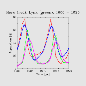
where and denote the population number of the prey and the predator, respectively. Here, the coupling constants describe the influence of the species on each other. We want to recover such a system from some historical data of numbers of lynxes (predator) and hares (prey), collected by the Hudson Bay Company in Canada during the years –. This data set can be seen, more or less, as representative for the total population number of both species [1].
For basic biological reasons a constant term is missing in both components of the anticipated predator-prey model (3.2)–(3.3). Hence, we exclude the constant monomial term in both reconstruction runs as well. The maximal degree of the multi-variate polynomials is set to 3.
(a) 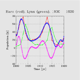 (b)
(b) 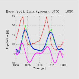
Runtime protocol for component.
#total = 16 (max. deg. 3) [ 0 2 ] --> [0, 1] 100.00 % c_k = 8.999962e-01 [ 0 3 ] --> [0, 2] 3.79 % c_k = -3.408105e-02 [ 0 4 ] --> [0, 3] 0.00 % c_k = 1.703492e-04 [ 1 2 ] --> [1, 0] 19.66 % c_k = -1.769268e-01 [ 1 3 ] --> [1, 1] 3.44 % c_k = -3.092972e-02 [ 1 4 ] --> [1, 2] 0.00 % c_k = 3.976574e-04 [ 2 3 ] --> [2, 0] 2.65 % c_k = 2.384418e-02 [ 2 4 ] --> [2, 1] 0.00 % c_k = -4.353977e-05 [ 3 4 ] --> [3, 0] 0.00 % c_k = -2.065367e-04 m = 9 monomial(s) 0.10 % threshold f(y0,y1) = + ( 9.0e-01) y1^1 + (-3.4e-02) y1^2 + (-1.8e-01) y0^1 + (-3.1e-02) y0^1 y1^1 + ( 2.4e-02) y0^2 LSQ: ||residual/sqrt(n)||_2 = 3.095545072754599
The is found to be described by the equation
| (3.4) |
with , , , , and .
(a) 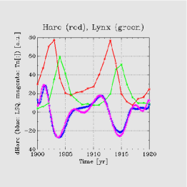 (b)
(b) 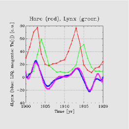
Runtime protocol for component.
#total = 16 (max. deg. 3) [ 0 2 ] --> [0, 1] 100.00 % c_k = -1.590145e+00 [ 0 3 ] --> [0, 2] 1.35 % c_k = 2.146557e-02 [ 0 4 ] --> [0, 3] 0.00 % c_k = 1.283903e-04 [ 1 2 ] --> [1, 0] 45.70 % c_k = 7.266958e-01 [ 1 3 ] --> [1, 1] 0.87 % c_k = 1.379691e-02 [ 1 4 ] --> [1, 2] 0.00 % c_k = -4.190196e-04 [ 2 3 ] --> [2, 0] 1.35 % c_k = -2.140643e-02 [ 2 4 ] --> [2, 1] 0.00 % c_k = 2.619544e-04 [ 3 4 ] --> [3, 0] 0.00 % c_k = 1.834174e-04 m = 9 monomial(s) 0.10 % threshold f(y0,y1) = + (-1.6e+00) y1^1 + ( 2.1e-02) y1^2 + ( 7.3e-01) y0^1 + ( 1.4e-02) y0^1 y1^1 + (-2.1e-02) y0^2 LSQ: ||residual/sqrt(n)||_2 = 3.1046555639780498
Here, the component is found to be given by the equation
| (3.5) |
with , , , , and .
It would be interesting to see if an additional, iterative Gauss-Newton fit would improve the identified parameters further and, possibly, establish some link to the standard predator-prey model (3.2)–(3.3). Unfortunately, for the case with multi-variate polynomials of maximal degree 3, as presented here, such an additional verification has not been successful at all. Instead, the Gauss-Newton iteration stops after a few steps with the ODE system being not integrable any more, i.e. the Newton path of the coefficient sets during the iteration inexplicably leads to an ODE system that can not be solved numerically. A systematic and comprehensive investigation of this unexpected behaviour would certainly go beyond the scope of this article and hence, must be left open for now.
However, a repeated computation, completely analogous to the one presented here, only with the maximal polynomial degree restricted to 2, nicely demonstrates a relationship to the standard predator-prey model, as we have previously gathered, see Table 1. In particular, there is an intriguing match between the coefficients of the second component, i.e. the ODE equation of the lynx. The incompatibility factor in the last row of Table 1 is determined by the ratio of the norms of successive updates during the Gauss-Newton iteration and thus, can be seen as an estimate of the convergence speed, especially at the end of the iteration. This factor, if strictly below , can be thought to measure how compatible a model to given data is (see [12, sec. 4.3.2] for the mathematical background). The values in the last column of Table 1 can be found in [1]. All the computational details are given in the Appendix.
-
Component Multi-index Data-based Standard 1.848730e-01 3.675366e-03 2.531473e-01 5.475337e-01 () -3.789005e-02 -2.811932e-02 () 7.856857e-03 -9.587181e-01 -8.431750e-01 () 6.845210e-04 5.296776e-02 2.408610e-02 2.655759e-02 () -1.113486e-04 Scaled residual (Normf) 3.0712e-00 4.2362e-00 (incomp. factor, see [12]) 1.0274e-01 2.9798e-02
To sum up the hare and lynx case, the reconstructed components and seem to follow only partly the standard predator-prey model. Instead, our findings here show that the data might be more involved than previously assumed. Our conclusion is also supported by the verification result, as can be seen in Figure 3.
3.2 Damped Pendulum
Here, we consider the initial value problem
| (3.6) | |||||
| (3.7) |
with the initial condition , and the constants , , and (the gravitational acceleration on earth) are used [2]. Very sparse data has been generated by solving numerically (3.6)–(3.7) in the time interval , and subsequently taking equidistant samples of the solution trajectories in this interval.
In order to be able to catch a glimpse of the non-linearity on the right-hand side in (3.7), for the reconstruction trial the maximal degree of the multi-variate polynomials is set to .
(a) 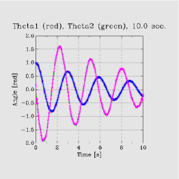 (b)
(b) 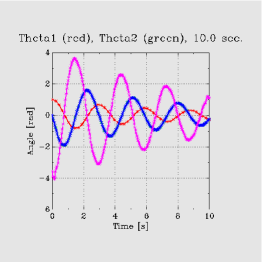
As seen in the following runtime protocol for the component, the equation
| (3.8) |
with is found.
Runtime protocol for component.
#total = 25 (max. deg. 4) [ 0 1 ] --> [0, 0] 0.00 % c_k = 2.001792e-03 [ 0 2 ] --> [0, 1] 100.00 % c_k = 9.982190e-01 [ 0 3 ] --> [0, 2] 0.00 % c_k = -6.094577e-03 [ 0 4 ] --> [0, 3] 0.00 % c_k = -2.859434e-04 [ 0 5 ] --> [0, 4] 0.00 % c_k = 1.027003e-03 [ 1 2 ] --> [1, 0] 0.00 % c_k = 1.384047e-03 [ 1 3 ] --> [1, 1] 0.00 % c_k = 2.514082e-02 [ 1 4 ] --> [1, 2] 0.00 % c_k = 4.947748e-03 [ 1 5 ] --> [1, 3] 0.00 % c_k = -5.810996e-03 [ 2 3 ] --> [2, 0] 0.00 % c_k = -2.636188e-02 [ 2 4 ] --> [2, 1] 0.00 % c_k = 3.051582e-02 [ 2 5 ] --> [2, 2] 0.00 % c_k = 2.399808e-02 [ 3 4 ] --> [3, 0] 0.00 % c_k = -2.561132e-03 [ 3 5 ] --> [3, 1] 0.00 % c_k = -1.691789e-02 [ 4 5 ] --> [4, 0] 0.00 % c_k = 3.776657e-02 m = 15 monomial(s) 5.00 % threshold f(y0,y1) = + ( 1.0e+00) y1^1 LSQ: ||residual/sqrt(n)||_2 = 0.035592552825152
(a) 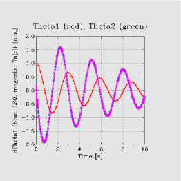 (b)
(b) 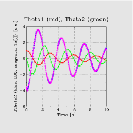
Runtime protocol for component.
#total = 25 (max. deg. 4) [ 0 1 ] --> [0, 0] 0.00 % c_k = 5.555385e-03 [ 0 2 ] --> [0, 1] 5.13 % c_k = -2.535032e-01 [ 0 3 ] --> [0, 2] 0.00 % c_k = -1.796957e-02 [ 0 4 ] --> [0, 3] 0.00 % c_k = -6.444822e-03 [ 0 5 ] --> [0, 4] 0.00 % c_k = -3.850649e-04 [ 1 2 ] --> [1, 0] 100.00 % c_k = -4.942789e+00 [ 1 3 ] --> [1, 1] 0.00 % c_k = -1.564249e-01 [ 1 4 ] --> [1, 2] 0.00 % c_k = 2.928157e-02 [ 1 5 ] --> [1, 3] 0.00 % c_k = 1.852611e-02 [ 2 3 ] --> [2, 0] 0.00 % c_k = -9.883681e-02 [ 2 4 ] --> [2, 1] 0.00 % c_k = 1.441293e-01 [ 2 5 ] --> [2, 2] 0.00 % c_k = 1.787311e-01 [ 3 4 ] --> [3, 0] 19.50 % c_k = 9.639487e-01 [ 3 5 ] --> [3, 1] 9.90 % c_k = 4.893068e-01 [ 4 5 ] --> [4, 0] 0.00 % c_k = 2.128485e-01 m = 15 monomial(s) 5.00 % threshold f(y0,y1) = + (-2.5e-01) y1^1 + (-4.9e+00) y0^1 + ( 9.6e-01) y0^3 + ( 4.9e-01) y0^3 y1^1 LSQ: ||residual/sqrt(n)||_2 = 0.04531770760243261
In this case, for the component, we obtain
| (3.9) |
with , , , and .
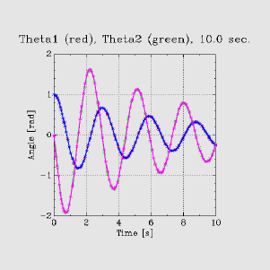
Summarising these findings, the recovered equations in this non-linear case agree convincingly well with the pendulum model that has been used to generated the given sparse data set. Especially for the second component , the reconstructed coefficients and match the Taylor coefficients of the sine in the right-hand side of the original damped pendulum model. The discrepancy in is compensated by the additional coefficient , indicating that the approximated model is still not complete. Nevertheless, the verification result, as can be seen clearly in Figure 6, is already almost perfect.
4 Conclusion
In the present paper, a highly flexible method for the reconstruction of an unknown dynamical system, to be described in terms of an explicit ODE system, is presented. The reconstruction method is based on sampled, possibly sparse, trajectory solution points as given data.
In principle, any kind of relationship between the available information is tried to be recovered automatically, if different components of the unknown system are given. Yet, because of the extreme simple structure of the presented method, and the fact that the ODE itself is not being solved during the reconstruction, it is possible to readily adapt the approach to any anticipated behaviour of the unknown dynamical system. Moreover, the approach is fast and, most importantly, highly reliable.
Additionally, the results of our fast reconstruction method could be used as a very good starting guess, for example, of more sophisticated iterative identification procedures such as well-established Gauss-Newton codes [12].
Appendix
Here, we repeat the computations of section 3.1 for the predator-prey case, only the maximal degree of the multi-variate polynomials is set to 2. This results in the following two runtime protocols.
Runtime protocol for component.
#total = 9 (max. deg. 2) [ 0 2 ] --> [0, 1] 7.72 % c_k = -3.591668e-02 [ 0 3 ] --> [0, 2] 0.93 % c_k = -4.319190e-03 [ 1 2 ] --> [1, 0] 100.00 % c_k = 4.653563e-01 [ 1 3 ] --> [1, 1] 3.58 % c_k = -1.665442e-02 [ 2 3 ] --> [2, 0] 0.00 % c_k = -9.424325e-05 m = 5 monomial(s) 0.10 % threshold f(y0,y1) = + (-3.6e-02) y1^1 + (-4.3e-03) y1^2 + ( 4.7e-01) y0^1 + (-1.7e-02) y0^1 y1^1 LSQ: ||residual/sqrt(n)||_2 = 3.7658055884421944
Runtime protocol for component.
#total = 9 (max. deg. 2) [ 0 2 ] --> [0, 1] 100.00 % c_k = -9.800874e-01 [ 0 3 ] --> [0, 2] 0.68 % c_k = 6.673957e-03 [ 1 2 ] --> [1, 0] 7.26 % c_k = 7.117392e-02 [ 1 3 ] --> [1, 1] 1.52 % c_k = 1.487619e-02 [ 2 3 ] --> [2, 0] 0.16 % c_k = 1.545017e-03 m = 5 monomial(s) 0.10 % threshold f(y0,y1) = + (-9.8e-01) y1^1 + ( 6.7e-03) y1^2 + ( 7.1e-02) y0^1 + ( 1.5e-02) y0^1 y1^1 + ( 1.5e-03) y0^2 LSQ: ||residual/sqrt(n)||_2 = 3.666500740586521
Taking these coefficients and , , as starting values for an non-linear least squares method, in order to identify parameters of the ODE model build by these two polynomials
| (1.1) | |||||
| (1.2) |
with initial conditions and kept fixed, will result in a runtime protocol as follows, trying to match the given measurement data best in the least squares sense by successively varying these 10 coefficients. Here, we choose an error-oriented Gauss-Newton scheme with adaptive trust region and rank strategy, NLSCON, as fitting routine. Solutions to the IVP of (1.1)–(1.2) are computed by the linearly-implicit extrapolation integrator LIMEX [13, 14] during the Gauss-Newton iteration, with and . All other relevant settings are included in the resulting runtime protocol of the parameter identification task for the data-based model (1.1)–(1.2).
Runtime protocol for an error-oriented Gauss-Newton scheme (NLSCON).
N L S C O N ***** V e r s i o n 2 . 3 . 3 *** Gauss-Newton-Method for the solution of nonlinear least squares problems Real Workspace declared as 1742 is used up to 1578 ( 90.6 percent) Integer Workspace declared as 62 is used up to 50 ( 80.6 percent) Number of parameters to be estimated (N) : 10 Number of data to fitted, e.g. observations (MFIT) : 42 Number of equality constraints (MCON) : 0 Prescribed relative precision (PTOL) : 0.10D-02 The Jacobian is supplied by numerical differentiation (feedback strategy included) Automatic row scaling of the Jacobian is allowed Rank-1 updates are inhibited Problem is specified as being highly nonlinear Bounded damping strategy is off Maximum permitted number of iteration steps : 40 Internal parameters: Starting value for damping factor FCSTART = 0.10D-01 Minimum allowed damping factor FCMIN = 0.10D-01 Rank-1 updates decision parameter SIGMA = 0.10D+04 Initial Jacobian pseudo-rank IRANK = 10 Maximum permitted subcondition COND = 0.45D+16 *********************************************************************** It Normf Normx Damp.Fct. New Rank 0 0.8345461D+01 0.251D+00 0 10 1 0.8277889D+01 * 0.248D+00 0.010 1 1 0.8277889D+01 0.241D+00 0 10 2 0.5289067D+01 * 0.916D-01 0.375 2 2 0.5289067D+01 0.991D-01 0 10 2 0.9455332D+01 * 0.133D+00 0.819 3 0.4570706D+01 * 0.755D-01 0.232 3 3 0.4570706D+01 0.827D-01 0 10 4 0.6342464D+01 * 0.732D-01 1.000 4 4 0.6342464D+01 0.229D-01 0 10 5 0.3444394D+01 * 0.723D-02 1.000 5 5 0.3444394D+01 0.171D-01 0 10 6 0.3083738D+01 * 0.315D-02 0.955 6 6 0.3083738D+01 0.652D-02 0 10 7 0.3071453D+01 * 0.120D-03 1.000 7 7 0.3071453D+01 0.176D-02 0 10 8 0.3071223D+01 * 0.252D-05 1.000 8 8 0.3071223D+01 0.180D-03 0 10 9 0.3071220D+01 * 0.957D-07 1.000 Solution of nonlinear least squares problem obtained within 9 iteration steps Incompatibility factor kappa 0.103D+00 Achieved relative accuracy 0.207D-04
Additional statistical analysis of the result of the identification task.
Standard deviation of parameters -------------------------------- No. Estimate sigma(X) 1 0.185D+00 +/- 0.174D+00 = 94.25 % 2 0.368D-02 +/- 0.463D-02 = 125.87 % 3 0.253D+00 +/- 0.107D+00 = 42.40 % 4 -0.379D-01 +/- 0.646D-02 = 17.04 % 5 0.786D-02 +/- 0.271D-02 = 34.46 % 6 -0.959D+00 +/- 0.198D+00 = 20.67 % 7 0.685D-03 +/- 0.491D-02 = 716.79 % 8 0.530D-01 +/- 0.725D-01 = 136.89 % 9 0.241D-01 +/- 0.465D-02 = 19.29 % 10 -0.111D-03 +/- 0.124D-02 = 1109.90 % Independent confidence intervals -------------------------------- (on 95%-probability level using F-distribution F(alfa,1,m-n)= 4.15) 1 ( -0.170D+00 , 0.540D+00 ) 2 ( -0.575D-02 , 0.131D-01 ) 3 ( 0.345D-01 , 0.472D+00 ) 4 ( -0.510D-01 , -0.247D-01 ) 5 ( 0.234D-02 , 0.134D-01 ) 6 ( -0.136D+01 , -0.555D+00 ) 7 ( -0.931D-02 , 0.107D-01 ) 8 ( -0.947D-01 , 0.201D+00 ) 9 ( 0.146D-01 , 0.336D-01 ) 10 ( -0.263D-02 , 0.241D-02 ) ****** Statistics * NLSCON ******* *** Gauss-Newton iter.: 9 *** *** Corrector steps : 1 *** *** Rejected rk-1 st. : 0 *** *** Jacobian eval. : 10 *** *** Function eval. : 12 *** *** ... for Jacobian : 100 *** *************************************
In order to have a visual inspection of these findings, the resulting population curves are plotted in Figure 7. In particular it seems that the curves of our approximated model match more the given data in the time period 1905 – 1915.
Note that, although the Gauss-Newton iteration converges nicely, and with full rank of the Jacobians, the overall estimated standard deviation of the identified coefficients is relatively high. This means that the linearisation at the minimum point found is nearly flat and hence, the corresponding confidence intervals are comparatively wide.
(a) 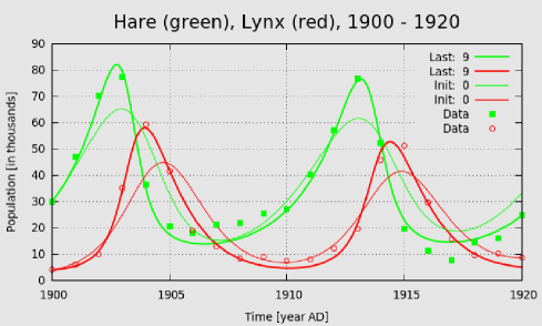
(b) 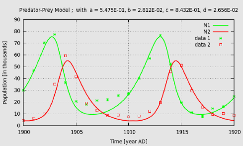
The implementation of the presented approach that, written in Ruby, has been applied to perform all example computations in this paper is available upon request.
References
- [1] Deuflhard P and Röblitz S 2015 A Guide to Numerical Modelling in Systems Biology (Texts in Computational Science and Engineering no 12) (Springer-Verlag)
- [2] Perona P, Porporato A and Ridolfi L 2000 Nonlinear Dynamics 23 13–33
- [3] Walter E and Pronzato L 1997 Identification of Parametric Models from Experimental Data (Springer)
- [4] Deuflhard P and Bornemann F 2002 Scientific Computing with Ordinary Differential Equations 1st ed (Texts in Applied Mathematics no 42) (Springer-Verlag)
- [5] Eisenhammer T, Hübler A, Packard N and Kelso J 1991 Biological Cybernetics 65 107–112
- [6] Raue A, Steiert B, Schelker M, Kreutz C, Maiwald T, Hass H, Vanlier J, Tönsing C, Adlung L, Engesser R, Mader W, Heinemann T, Hasenauer J, Schilling M, Höfer T, Klipp E, Theis F, Klingmüller U, Schöberl B and Timmer J 2015 Bioinformatics 31 3558–3560
- [7] Press W H, Teukolsky S A, Vetterling W T and Flannery B P 2002 Numerical Recipes in C++ : The Art of Scientific Computing 2nd ed (Cambridge University Press)
- [8] Trefethen L 2013 Approximation Theory and Approximation Practice (Philadelphia, PA: Society for Industrial and Applied Mathematics (SIAM)) URL http://www2.maths.ox.ac.uk/chebfun/ATAP/
- [9] Quarteroni A, Sacco R and Saleri F 2007 Numerical Mathematics 2nd ed (Texts in Applied Mathematics no 37) (Springer-Verlag)
- [10] De Boor C 1978 A Practical Guide to Splines (New York: Springer-Verlag)
- [11] Deuflhard P and Hohmann A 2003 Numerical analysis in Modern Scientific Computing – An Introduction 2nd ed (Texts in Applied Mathematics no 43) (Springer-Verlag)
- [12] Deuflhard P 2004 Newton Methods for Nonlinear Problems – Affine Invariance and Adaptive Algorithms (Springer Series in Computational Mathematics no 35) (Springer)
- [13] Ehrig R, Nowak U, Oeverdieck L and Deuflhard P 1999 Lecture Notes in Computational Science and Engineering 8 233–244
- [14] Deuflhard P and Nowak U 1987 Extrapolation integrators for quasilinear implicit ODEs Large Scale Scientific Computing ed Deuflhard P and Engquist B (Birkhäuser) pp 37–50