Sensitivity analysis, multilinearity and beyond

Manuele Leonelli Departamento de Estatística, Universidade Federal do Rio de Janeiro, Rio de Janeiro, Brazil Christiane Görgen and Jim Q. Smith Department of Statistics, The University of Warwick, Coventry, UK
Abstract

Sensitivity methods for the analysis of the outputs of discrete Bayesian networks have been extensively studied and implemented in different software packages. These methods usually focus on the study of sensitivity functions and on the impact of a parameter change to the Chan-Darwiche distance. Although not fully recognized, the majority of these results rely heavily on the multilinear structure of atomic probabilities in terms of the conditional probability parameters associated with this type of network. By defining a statistical model through the polynomial expression of its associated defining conditional probabilities, we develop here a unifying approach to sensitivity methods applicable to a large suite of models including extensions of Bayesian networks, for instance context-specific and dynamic ones. Our algebraic approach enables us to prove that for models whose defining polynomial is multilinear both the Chan-Darwiche distance and any divergence in the family of ϕitalic-ϕ\phi-divergences are minimized for a certain class of multi-parameter contemporaneous variations when parameters are proportionally covaried.

keywords:
Bayesian networks , CD distance , Interpolating Polynomial , Sensitivity Analysis , ϕitalic-ϕ\phi-divergences.

1 Introduction

Many discrete statistical problems in a variety of domains are nowadays often modeled using Bayesian networks (BNs) [38]. There are now thousands of practical applications of these models [1, 7, 27, 29], which have spawned many useful technical developments: including a variety of fast exact, approximate and symbolic propagation algorithms for the computation of probabilities that exploit the underlying graph structure [17, 19, 20]. Some of these advances have been hard-wired into software [9, 31, 34] which has further increased the applicability and success of these methods.

However, BN modeling would not have experienced such a widespread application without tailored methodologies of model validation, i.e. checking that a model produces outputs that are in line with current understanding, following a defensible and expected mechanism [22, 41]. Such techniques are now well established for BN models [15, 31, 41, 42]. These are especially fundamental for expert elicited models, where both the probabilities and the covariance structure are defined from the suggestions of domains experts, following knowledge engineering protocols tailored to the BN’s bulding process [36, 43]. We can broadly break down the validation process into two steps: the first concerns the auditing of the underlying graphical structure; the second, assuming the graph represents a user’s beliefs, checks the impact of the numerical elicited probabilities within this parametric family on outputs of interest. The focus of this paper lies in this second validation phase, usually called a sensitivity analysis.

The most common investigation is the so-called one-way sensitivity analysis, where the impacts of changes made to a single probability parameter are studied. Analyses where more than one parameter at a time is varied are usually referred to as multi-way. In both cases a complete sensitivity analysis for discrete BNs often involves the study of Chan-Darwiche (CD) distances [9, 10, 11] and sensitivity functions [16, 48]. The CD distance is used to quantify global changes. It measures how the overall distribution behaves when one (or more) parameter is varied. A significant proportion of research has focused on identifying parameter changes such that the original and the ‘varied’ BN distributions are close in CD distance [11, 45]. This is minimized when, after a single arbitrary parameter change, other covarying parameters, e.g. those from the same conditional distribution, have the same proportion of the residual probability mass as they originally had. Sensitivity functions, on the other hand, model local changes with respect to an output of interest. These describe how that output probability varies as one (or potentially more) parameter is allowed to be changed. Although both these concepts can be applied to generic Bayesian analyses, they have almost exclusively been discussed and applied only within the BN literature (see [12, 13, 14, 44] for some exceptions). This is because the computations of both CD distances and sensitivity functions are particularly straightforward for BN models.

In this paper we introduce a unifying comprehensive framework for certain multi-way analyses, usually called in the context of BNs single full conditional probability table (CPT) analyses - where one parameter from each CPT of one vertex of a BN given each configurations of its parents is varied. Using the notion of an interpolating polynomial [40] we are able to describe a large variety of models based on their polynomial form. Then, given this algebraic carachterization, we demonstrate that one-way sensitivity methods defined for BNs can be generalized to single full CPT analyses for any model whose interpolating polynomial is multilinear, for example context-specific BNs [6] and chain event graphs [47]. Because of both the lack of theoretical results justifying their use and the increase in computational complexity, multi-way methods have not been extensively discussed in the literature: see [5, 10, 24] for some exceptions. This paper aims at providing a comprehensive theoretical toolbox to start applying such analyses in practice.

Importantly, our polynomial approach enables us to prove that single full CPT analyses in any multilinear polynomial model are optimal under proportional covariation in the sense that the CD distance between the original and the varied distributions is minimized. The optimality of this covariation method has been an open problem in the sensitivity analysis literature for quite some time [10, 45]. However, we are able to provide further theoretical justifications for the use of proportional covariation in single full CPT analyses. We demonstrate below that for any multilinear model this scheme minimizes not only the CD distance, but also any divergence in the family of ϕitalic-ϕ\phi-divergences [2, 18]. The class of ϕitalic-ϕ\phi-divergences include a very large number of divergences and distances (see e.g. [37] for a review), including the famous Kullback-Leibler (KL) divergence [32]. The application of KL distances in sensitivity analyses of BNs has been almost exclusively restricted to the case when the underlying distribution is assumed Gaussian [23, 24], because in discrete BNs the computation of such a divergence requires more computational power than for CD distances. We will demonstrate below that this additional complexity is a feature shared by any divergence in the family of ϕitalic-ϕ\phi-divergences.

However, by studying sensitivity analysis from a polynomial point of view, we are able to consider a much larger class of models for which such methods are very limited. We investigate the properties of one-way sensitivity analysis in models whose interpolating polynomial is not multilinear, which are usually associated to dynamic settings where probabilities are recursively defined. This difference gives us an even richer class of sensitivity functions as shown in [13, 14, 44] for certain dynamic BN models, which are not simply linear but more generally polynomial. We further introduce a procedure to compute the CD distance in these models and demonstrate that no unique updating of covarying parameters lead to the smallest CD distance between the original and the varied distribution.

The paper is structured as follows. In Section 2 we define interpolating polynomials and demonstrate that many commonly used models entertain a polynomial representation. In Section 3 we review a variety of divergence measures. Section 4 presents a variety of results for single full CPT sensitivity analyses in multilinear models. In Section 5 the focus moves to non-multilinear models and one-way analyses. We conclude with a discussion.

2 Multilinear and polynomial parametric models

In this section we first provide a generic definition of a parametric statistical model together with the notion of interpolating polynomial. We then categorize parametric models according to the form of their interpolating polynomial and show that many commonly used models fall within two classes.

2.1 Parametric models and interpolating polynomials

Let 𝒀=(Y1,,Ym)𝒀subscript𝑌1subscript𝑌𝑚\bm{Y}=(Y_{1},\dots,Y_{m}) be a random vector with an associated discrete and finite sample space 𝕐𝕐\bm{\mathbb{Y}}, with #𝕐=n#𝕐𝑛\#\mathbb{Y}=n. Although our methods straightforwardly applies when the entries of 𝒀𝒀\bm{Y} are random vectors, for ease of notation, we henceforth assume its elements are univariate.

Definition 1.

Denote by 𝐩θ=(pθ(𝐲)|𝐲𝕐)subscript𝐩𝜃conditionalsubscript𝑝𝜃𝐲𝐲𝕐\bm{p}_{\theta}=(p_{\theta}(\bm{y})~{}|~{}\bm{y}\in\bm{\mathbb{Y}}) the vector of values of a probability mass function pθ:𝕐[0,1]:subscript𝑝𝜃𝕐01p_{\theta}:\bm{\mathbb{Y}}\to[0,1] which depends on a choice of parameters θk𝜃superscript𝑘\theta\in\mathbb{R}^{k}. The entries of 𝐩θsubscript𝐩𝜃\bm{p}_{\theta} are called atomic probabilities and the elements 𝐲𝕐𝐲𝕐\bm{y}\in\bm{\mathbb{Y}} atoms.

Definition 2.

A discrete parametric statistical model on n𝑛n\in\mathbb{N} atoms is a subset ΨΔn1subscriptΨsubscriptΔ𝑛1\mathbb{P}_{\Psi}\subseteq\Delta_{n-1} of the n1𝑛1n-1 dimensional probability simplex, where

Ψ:kΨ,θ𝒑θ,\Psi~{}:\quad\mathbb{R}^{k}\to\mathbb{P}_{\Psi},~{}\theta\mapsto\bm{p}_{\theta}, (1)

is a bijective map identifying a particular choice of parameters θk𝜃superscript𝑘\theta\in\mathbb{R}^{k} with one vector of atomic probabilities. The map ΨΨ\Psi is called a parametrisation of the model.

The above definition is often encountered in the field of algebraic statistics, where properties of statistical models are studied using techniques from algebraic geometry and commutative computer algebra, among others [21, 46]. We next follow [25] in extending some standard terminology.

Definition 3.

A model ΨΔn1subscriptΨsubscriptΔ𝑛1\mathbb{P}_{\Psi}\subseteq\Delta_{n-1} has a monomial parametrisation if

pθ(𝒚)=𝜽𝜶𝒚,for all 𝒚𝕐,formulae-sequencesubscript𝑝𝜃𝒚superscript𝜽subscript𝜶𝒚for all 𝒚𝕐p_{\theta}(\bm{y})=\bm{\theta}^{\bm{\alpha}_{\bm{y}}},\quad\text{for all }\bm{y}\in\bm{\mathbb{Y}},

where 𝛂𝐲0ksubscript𝛂𝐲superscriptsubscript0𝑘\bm{\alpha}_{\bm{y}}\in\mathbb{N}_{0}^{k} denotes a vector of exponents and 𝛉𝛂𝐲=θ1α1,𝐲θkαk,𝐲superscript𝛉subscript𝛂𝐲superscriptsubscript𝜃1subscript𝛼1𝐲superscriptsubscript𝜃𝑘subscript𝛼𝑘𝐲\bm{\theta}^{\bm{\alpha}_{\bm{y}}}=\theta_{1}^{\alpha_{1,\bm{y}}}\cdots\theta_{k}^{\alpha_{k,\bm{y}}} is a monomial. Then equation (1) is a monomial map and 𝛉𝛂𝐲k[Θ]superscript𝛉subscript𝛂𝐲subscript𝑘delimited-[]Θ\bm{\theta}^{\bm{\alpha}_{\bm{y}}}\in\mathbb{R}_{k}[\Theta], for all 𝐲𝕐𝐲𝕐\bm{y}\in\mathbb{Y}. Here Θ={θ1,,θk}Θsubscript𝜃1subscript𝜃𝑘\Theta=\{\theta_{1},\ldots,\theta_{k}\} is the set of indeterminates and k[Θ]subscript𝑘delimited-[]Θ\mathbb{R}_{k}[\Theta] is the polynomial ring over the field \mathbb{R}.

For models entertaining a monomial parametrisation the network polynomial we introduce in Definition 4 below concisely captures the model structure and provides a platform to answer inferential queries [20, 26].

Definition 4.

The network polynomial of a model ΨsubscriptΨ\mathbb{P}_{\Psi} with monomial parametrisation ΨΨ\Psi is given by

cΨ(θ,λ)=𝒚𝕐λ𝒚𝜽𝜶𝒚,subscript𝑐subscriptΨ𝜃𝜆subscript𝒚𝕐subscript𝜆𝒚superscript𝜽subscript𝜶𝒚c_{\mathbb{P}_{\Psi}}(\theta,\lambda)=\sum_{\bm{y}\in\bm{\mathbb{Y}}}\lambda_{\bm{y}}\bm{\theta}^{\bm{\alpha}_{\bm{y}}},

where λ𝐲subscript𝜆𝐲\lambda_{\bm{y}} is an indicator function for the atom 𝐲𝐲\bm{y}.

Probabilities of events in the underlying sigma-field can be computed from the network polynomial by setting equal to one the indicator function of atoms associated to that event. In the following it will be convenient to work with a special case of the network polynomial where all the indicator functions are set to one.

Definition 5.

The interpolating polynomial of a model ΨsubscriptΨ\mathbb{P}_{\Psi} with monomial parametrisation ΨΨ\Psi is given by the sum of all atomic probabilities,

cΨ(θ)=𝜶𝔸𝜽𝜶,subscript𝑐subscriptΨ𝜃subscript𝜶𝔸superscript𝜽𝜶c_{\mathbb{P}_{\Psi}}(\theta)=\sum_{\bm{\alpha}\in\bm{\mathbb{A}}}\bm{\theta}^{\bm{\alpha}},

where 𝔸={𝛂𝐲|𝐲𝕐}0k𝔸conditional-setsubscript𝛂𝐲𝐲𝕐subscriptsuperscript𝑘0\mathbb{A}=\{\bm{\alpha}_{\bm{y}}\ |\ \bm{y}\in\mathbb{Y}\}\subset\mathbb{N}^{k}_{0}.

2.2 Multilinear models

In this work we will mostly focus on parametric models whose interpolating polynomial is multilinear.

Definition 6.

We say that a parametric model ΨsubscriptΨ\mathbb{P}_{\Psi} is multilinear if its associated interpolating polynomial is multilinear, i.e. if 𝔸{0,1}k𝔸superscript01𝑘\mathbb{A}\subseteq\{0,1\}^{k}.

We note here that a great portion of well-known non-dynamic graphical models are multilinear. We explicitly show below that this is the case for BNs and context-specific BNs [6]. In [26] we showed that certain chain event graph models [47] have multilinear interpolating polynomial. In addition, decomposable undirected graphs and probabilistic chain graphs [33] can be defined to have a monomial parametrisation whose associated interpolating polynomial is multilinear. An example of models non entertaining a monomial parametrisation in terms of atomic probabilities are non-decomposable undirected graphs, since their joint distribution can be written as a rational function of multilinear functions [12].

2.2.1 Bayesian networks

For an m𝑚m\in\mathbb{N}, let [m]={1,,m}delimited-[]𝑚1𝑚[m]=\{1,\dots,m\}. We denote with Yisubscript𝑌𝑖Y_{i}, i[m]𝑖delimited-[]𝑚i\in[m], a generic discrete random variable and with 𝕐i={0,,mi}subscript𝕐𝑖0subscript𝑚𝑖\mathbb{Y}_{i}=\{0,\dots,m_{i}\} its associated sample space. For an A[m]𝐴delimited-[]𝑚A\subseteq[m], we let 𝒀A=(Yi)iAsubscript𝒀𝐴subscriptsubscript𝑌𝑖𝑖𝐴\bm{Y}_{A}=(Y_{i})_{i\in A} and 𝕐A=×iA𝕐i\bm{\mathbb{Y}}_{A}=\times_{i\in A}\mathbb{Y}_{i}. Recall that for three random vectors 𝒀isubscript𝒀𝑖\bm{Y}_{i}, 𝒀jsubscript𝒀𝑗\bm{Y}_{j} and 𝒀ksubscript𝒀𝑘\bm{Y}_{k}, we say that 𝒀isubscript𝒀𝑖\bm{Y}_{i} is conditional independent of 𝒀jsubscript𝒀𝑗\bm{Y}_{j} given 𝒀ksubscript𝒀𝑘\bm{Y}_{k}, and write 𝒀i𝒀j|𝒀kperpendicular-toabsentperpendicular-tosubscript𝒀𝑖conditionalsubscript𝒀𝑗subscript𝒀𝑘\bm{Y}_{i}\mathchoice{\mathrel{\hbox to0.0pt{$\displaystyle\perp$\hss}\mkern 2.0mu{\displaystyle\perp}}}{\mathrel{\hbox to0.0pt{$\textstyle\perp$\hss}\mkern 2.0mu{\textstyle\perp}}}{\mathrel{\hbox to0.0pt{$\scriptstyle\perp$\hss}\mkern 2.0mu{\scriptstyle\perp}}}{\mathrel{\hbox to0.0pt{$\scriptscriptstyle\perp$\hss}\mkern 2.0mu{\scriptscriptstyle\perp}}}\bm{Y}_{j}\;|\;\bm{Y}_{k}, if Pr(𝒀i=𝒚i|𝒀j=𝒚j,𝒀k=𝒀k)=Pr(𝒀i=𝒚i|𝒀k=𝒀k)Prsubscript𝒀𝑖conditionalsubscript𝒚𝑖subscript𝒀𝑗subscript𝒚𝑗subscript𝒀𝑘subscript𝒀𝑘Prsubscript𝒀𝑖conditionalsubscript𝒚𝑖subscript𝒀𝑘subscript𝒀𝑘\Pr(\bm{Y}_{i}=\bm{y}_{i}\;|\;\bm{Y}_{j}=\bm{y}_{j},\bm{Y}_{k}=\bm{Y}_{k})=\Pr(\bm{Y}_{i}=\bm{y}_{i}\;|\;\bm{Y}_{k}=\bm{Y}_{k}).

Definition 7.

A BN over a discrete random vector 𝐘[m]subscript𝐘delimited-[]𝑚\bm{Y}_{[m]} consists of

  • 1.

    m1𝑚1m-1 conditional independence statements of the form Yi𝒀[i1]|𝒀Πiperpendicular-toabsentperpendicular-tosubscript𝑌𝑖conditionalsubscript𝒀delimited-[]𝑖1subscript𝒀subscriptΠ𝑖Y_{i}\mathchoice{\mathrel{\hbox to0.0pt{$\displaystyle\perp$\hss}\mkern 2.0mu{\displaystyle\perp}}}{\mathrel{\hbox to0.0pt{$\textstyle\perp$\hss}\mkern 2.0mu{\textstyle\perp}}}{\mathrel{\hbox to0.0pt{$\scriptstyle\perp$\hss}\mkern 2.0mu{\scriptstyle\perp}}}{\mathrel{\hbox to0.0pt{$\scriptscriptstyle\perp$\hss}\mkern 2.0mu{\scriptscriptstyle\perp}}}\bm{Y}_{[i-1]}\;|\,\bm{Y}_{\Pi_{i}}, where Πi[i1]subscriptΠ𝑖delimited-[]𝑖1\Pi_{i}\subseteq[i-1];

  • 2.

    a directed acyclic graph (DAG) 𝒢𝒢\mathcal{G} with vertex set V(𝒢)={Yi:i[m]}𝑉𝒢conditional-setsubscript𝑌𝑖𝑖delimited-[]𝑚V(\mathcal{G})=\{Y_{i}:i\in[m]\} and edge set E(𝒢)={(Yi,Yj):j[m],iΠj}𝐸𝒢conditional-setsubscript𝑌𝑖subscript𝑌𝑗formulae-sequence𝑗delimited-[]𝑚𝑖subscriptΠ𝑗E(\mathcal{G})=\{(Y_{i},Y_{j}):j\in[m],i\in\Pi_{j}\};

  • 3.

    conditional probabilities θij𝝅=Pr(Yi=j|𝒀Πi=𝝅)subscript𝜃subscript𝑖𝑗𝝅Prsubscript𝑌𝑖conditional𝑗subscript𝒀subscriptΠ𝑖𝝅\theta_{i_{j}\bm{\pi}}=\Pr(Y_{i}=j\;|\;\bm{Y}_{\Pi_{i}}=\bm{\pi}) for every j𝕐i𝑗subscript𝕐𝑖j\in\mathbb{Y}_{i}, 𝝅𝕐Πi𝝅subscript𝕐subscriptΠ𝑖\bm{\pi}\in\bm{\mathbb{Y}}_{\Pi_{i}} and i[m]𝑖delimited-[]𝑚i\in[m].

The vector 𝒀Πisubscript𝒀subscriptΠ𝑖\bm{Y}_{\Pi_{i}}, i[m]𝑖delimited-[]𝑚i\in[m], includes the parents of the vertex Yisubscript𝑌𝑖Y_{i}, i.e. those vertices Yjsubscript𝑌𝑗Y_{j} such that there is an edge (Yj,Yi)subscript𝑌𝑗subscript𝑌𝑖(Y_{j},Y_{i}) in the DAG 𝒢𝒢\mathcal{G} of the BN.

From [10] we know that for any atom 𝒚𝕐[m]𝒚subscript𝕐delimited-[]𝑚\bm{y}\in\bm{\mathbb{Y}}_{[m]} its associated monomial in the network polynomial can be written as

pθ(𝒚)=𝒚{ij,𝝅}λijθij𝝅,subscript𝑝𝜃𝒚subscriptproductsimilar-to𝒚subscript𝑖𝑗𝝅subscript𝜆subscript𝑖𝑗subscript𝜃subscript𝑖𝑗𝝅p_{\theta}(\bm{y})=\prod_{\bm{y}\sim\{i_{j},\bm{\pi}\}}\lambda_{i_{j}}\theta_{i_{j}\bm{\pi}},

where similar-to\sim denotes the compatibility relation among instantiations.

Lemma 1.

From [20, 26], the interpolating polynomial of a BN model can be written as

cBN(θ)=𝒚𝕐[m]𝒚{ij,𝝅}θij𝝅.subscript𝑐BN𝜃subscript𝒚subscript𝕐delimited-[]𝑚subscriptproductsimilar-to𝒚subscript𝑖𝑗𝝅subscript𝜃subscript𝑖𝑗𝝅c_{\textnormal{BN}}(\theta)=\sum_{\bm{y}\in\bm{\mathbb{Y}}_{[m]}}\prod_{\bm{y}\sim\{i_{j},\bm{\pi}\}}\theta_{i_{j}\bm{\pi}}. (2)

From Equation (2) we can immediately deduce the following.

Proposition 1.

A BN is a multilinear parametric model, whose interpolating polynomial is homogeneous with monomials of degree m𝑚m.

Example 1.

Suppose a newborn is at risk of acquiring a disease and her parents are offered a screening test (Y1subscript𝑌1Y_{1}) which can be either positive (Y1=1subscript𝑌11Y_{1}=1) or negative (Y1=0subscript𝑌10Y_{1}=0). Given that the newborn can either severely (Y2=2subscript𝑌22Y_{2}=2) or mildly (Y2=1subscript𝑌21Y_{2}=1) contract the disease or remain healthy (Y2=0subscript𝑌20Y_{2}=0), her parents can then decide whether or not to give her a vaccine to prevent a relapse (Y3=1subscript𝑌31Y_{3}=1 and Y3=0subscript𝑌30Y_{3}=0, respectively). We assume that the parents’ decision about the vaccine does not depend on the screening test if the newborn contracted the disease, and that the probability of being severely or mildly affected by the disease is equal for negative screening tests.

Y1subscriptY1\textstyle{Y_{1}\ignorespaces\ignorespaces\ignorespaces\ignorespaces\ignorespaces\ignorespaces\ignorespaces\ignorespaces\ignorespaces}Y2subscriptY2\textstyle{Y_{2}\ignorespaces\ignorespaces\ignorespaces\ignorespaces}Y3subscriptY3\textstyle{Y_{3}}

Figure 1: A BN model for the medical problem in Example 1.

The above situation can be described, with some loss of information, by the BN in Figure 1, with probabilities, for i,k{0,1}𝑖𝑘01i,k\in\{0,1\} and j{0,1,2}𝑗012j\in\{0,1,2\},

Pr(Y1=i)=θ1i,Pr(Y2=j|Y1=i)=θ2j1i,Pr(Y3=k|Y2=j,Y1=i)=θ3k2j1i.formulae-sequencePrsubscript𝑌1𝑖subscript𝜃subscript1𝑖formulae-sequencePrsubscript𝑌2conditional𝑗subscript𝑌1𝑖subscript𝜃subscript2𝑗subscript1𝑖Prsubscript𝑌3conditional𝑘subscript𝑌2𝑗subscript𝑌1𝑖subscript𝜃subscript3𝑘subscript2𝑗subscript1𝑖\Pr(Y_{1}=i)=\theta_{1_{i}},\quad\Pr(Y_{2}=j\,|\,Y_{1}=i)=\theta_{2_{j}1_{i}},\quad\Pr(Y_{3}=k\,|\,Y_{2}=j,Y_{1}=i)=\theta_{3_{k}2_{j}1_{i}}.

Its associated interpolating polynomial has degree 333 and equals

cBN(θ)=i=01j=02k=01θ1iθ2j1iθ3k2j1i.subscript𝑐BN𝜃superscriptsubscript𝑖01superscriptsubscript𝑗02superscriptsubscript𝑘01subscript𝜃subscript1𝑖subscript𝜃subscript2𝑗subscript1𝑖subscript𝜃subscript3𝑘subscript2𝑗subscript1𝑖c_{\textnormal{BN}}(\theta)=\sum_{i=0}^{1}\sum_{j=0}^{2}\sum_{k=0}^{1}\theta_{1_{i}}\theta_{2_{j}1_{i}}\theta_{3_{k}2_{j}1_{i}}.

2.2.2 Context-specific Bayesian networks

In practice it has been recognized that often conditional independence statements do not hold over the whole sample space of certain conditioning variables but only for a subset of this, usually referred to as a context. A variety of methods have been introduced to embellish a BN with additional independence statements that hold only over contexts. A BN equipped with such embellishments is usually called context-specific BN. Here we consider the representation known as context specific independence (CSI)-trees and introduced in [6].

Example 2.

Consider the medical problem in Example 1. Using the introduced notation, we notice that by assumption, for each k=0,1𝑘01k=0,1, the probabilities θ3k211isubscript𝜃subscript3𝑘subscript21subscript1𝑖\theta_{3_{k}2_{1}1_{i}} are equal for all i=0,1𝑖01i=0,1 and called θ3k211subscript𝜃subscript3𝑘subscript211\theta_{3_{k}2_{1}1}. Similarly, θ3k221isubscript𝜃subscript3𝑘subscript22subscript1𝑖\theta_{3_{k}2_{2}1_{i}} are equal and called θ3k221subscript𝜃subscript3𝑘subscript221\theta_{3_{k}2_{2}1}, i,k=0,1formulae-sequence𝑖𝑘01i,k=0,1. Also θ2210=θ2110subscript𝜃subscript22subscript10subscript𝜃subscript21subscript10\theta_{2_{2}1_{0}}=\theta_{2_{1}1_{0}} are equal and called θ210subscript𝜃subscript210\theta_{21_{0}}. The first two constraints can be represented by the CSI-tree in Figure 2, where the inner nodes are random variables and the leaves are entries of the CPTs of one vertex. The tree shows that, if Y2=1subscript𝑌21Y_{2}=1 or Y2=2subscript𝑌22Y_{2}=2 then no matter what the value of Y1subscript𝑌1Y_{1} is, the CPT for Y3=ksubscript𝑌3𝑘Y_{3}=k will be equal to θ3k211subscript𝜃subscript3𝑘subscript211\theta_{3_{k}2_{1}1} and θ3k211subscript𝜃subscript3𝑘subscript211\theta_{3_{k}2_{1}1} respectively.

Y2subscriptY2\textstyle{Y_{2}\ignorespaces\ignorespaces\ignorespaces\ignorespaces\ignorespaces\ignorespaces\ignorespaces\ignorespaces\ignorespaces\ignorespaces\ignorespaces\ignorespaces}11\scriptstyle{1}22\scriptstyle{2}00\scriptstyle{0}Y1subscriptY1\textstyle{Y_{1}\ignorespaces\ignorespaces\ignorespaces\ignorespaces\ignorespaces\ignorespaces\ignorespaces\ignorespaces}00\scriptstyle{0}11\scriptstyle{1}θ3k2010subscriptθsubscript3ksubscript20subscript10\textstyle{\theta_{3_{k}2_{0}1_{0}}}θ3k2011subscriptθsubscript3ksubscript20subscript11\textstyle{\theta_{3_{k}2_{0}1_{1}}}θ3k211subscriptθsubscript3ksubscript211\textstyle{\theta_{3_{k}2_{1}1}}θ3k221subscriptθsubscript3ksubscript221\textstyle{\theta_{3_{k}2_{2}1}}

Figure 2: CSI-tree associated to vertex Y3subscript𝑌3Y_{3} of the BN in Figure 1 of Example 1, where θ3k211=Pr(Y3=k|Y2=1)subscript𝜃subscript3𝑘subscript211Prsubscript𝑌3conditional𝑘subscript𝑌21\theta_{3_{k}2_{1}1}=\Pr(Y_{3}=k|Y_{2}=1), θ3k2011=Pr(Y3=k|Y2=0,Y1=1)subscript𝜃subscript3𝑘subscript20subscript11Prsubscript𝑌3conditional𝑘subscript𝑌20subscript𝑌11\theta_{3_{k}2_{0}1_{1}}=\Pr(Y_{3}=k|Y_{2}=0,Y_{1}=1) and θ3k201=Pr(Y3=k|Y1=0,Y2=0)=Pr(Y3|Y1=2,Y2=0)subscript𝜃subscript3𝑘subscript201Prsubscript𝑌3conditional𝑘subscript𝑌10subscript𝑌20Prconditionalsubscript𝑌3subscript𝑌12subscript𝑌20\theta_{3_{k}2_{0}1}=\Pr(Y_{3}=k|Y_{1}=0,Y_{2}=0)=\Pr(Y_{3}|Y_{1}=2,Y_{2}=0).

The last constraint cannot be represented by a CSI-tree and is usually referred to as a partial independence [39]. In our polynomial approach, both partial and context-specific independences can be straightforwardly imposed in the interpolating polynomial representation of the model. In fact the interpolating polynomial for the model in this example corresponds to the polynomial in equation (2) where the appropriate indeterminates are substituted with θ3k211subscript𝜃subscript3𝑘subscript211\theta_{3_{k}2_{1}1}, θ3k221subscript𝜃subscript3𝑘subscript221\theta_{3_{k}2_{2}1} and θ210subscript𝜃subscript210\theta_{21_{0}}. This polynomial is again multilinear and homogeneous, just like for all context-specific BNs embellished with CSI-trees and partial independences.

We notice here that the interpolating polynomial of a multilinear model is not necessarily homogenous, as for example the one associated to certain chain event graph models, as shown in [26].

2.3 Non-multilinear models

Having discussed multilinear models, we now introduce more general structures which are often encountered in dynamic settings. Although many more models have this property, for instance dynamic chain graphs [3] and dynamic chain event graphs [4], for the purposes of this paper we focus here on the most commonly used model class of dynamic Bayesian networks (DBNs) [35]. In [26] we showed that the so-called non square-free chain event graph is also a non-multilinear model.

2.3.1 Dynamic Bayesian networks

DBNs extend the BN framework to dynamic and stochastic domains. As often in practice, we consider only stationary, feed-forward DBNs respecting the first order Markov assumption with a finite horizon T𝑇T\in\mathbb{N}, see e.g. [30]. This assumes that probabilities do not vary when shifted on time (stationarity), that current states only depend on the previous time point (first-order Markov assumption) and that contemporaneous variable cannot directly affect each other (feed-forward). These DBNs can be simply described by an initial distribution over the first time point and a BN having as vertex set two generic time slices. Such latter BN is usually called 2-Time slice Bayesian Network (2-TBN). Let {𝒀(t)}t[T]={Yi(t):i[m]}t[T]subscript𝒀𝑡𝑡delimited-[]𝑇subscriptconditional-setsubscript𝑌𝑖𝑡𝑖delimited-[]𝑚𝑡delimited-[]𝑇\{\bm{Y}(t)\}_{t\in[T]}=\{Y_{i}(t):i\in[m]\}_{t\in[T]} be a time series.

Definition 8.

A 2-TBN for a time series {𝐘(t)}t[T]subscript𝐘𝑡𝑡delimited-[]𝑇\{\bm{Y}(t)\}_{t\in[T]} is a BN with DAG 𝒢𝒢\mathcal{G} such that V(𝒢)={Yi(t),Yi(t+1):i[m]}𝑉𝒢conditional-setsubscript𝑌𝑖𝑡subscript𝑌𝑖𝑡1𝑖delimited-[]𝑚V(\mathcal{G})=\{Y_{i}(t),Y_{i}(t+1):i\in[m]\} and its edge set is such that there are no edges (Yi(r),Yj(r))subscript𝑌𝑖𝑟subscript𝑌𝑗𝑟(Y_{i}(r),Y_{j}(r)), i,j[m]𝑖𝑗delimited-[]𝑚i,j\in[m], r=t,t+1𝑟𝑡𝑡1r=t,t+1, t[T1]𝑡delimited-[]𝑇1t\in[T-1].

Definition 9.

A DBN for a time series {𝐘(t)}t[T]subscript𝐘𝑡𝑡delimited-[]𝑇\{\bm{Y}(t)\}_{t\in[T]} is a pair (𝒢,𝒢)𝒢superscript𝒢(\mathcal{G},\mathcal{G}^{\prime}), such that 𝒢𝒢\mathcal{G} is a BN with vertex set V(𝒢)={Yi(1):i[m]}𝑉𝒢conditional-setsubscript𝑌𝑖1𝑖delimited-[]𝑚V(\mathcal{G})=\{Y_{i}(1):i\in[m]\}, and 𝒢superscript𝒢\mathcal{G}^{\prime} is a 2-TBN such that its vertex set V(𝒢)𝑉superscript𝒢V(\mathcal{G}^{\prime}) is equal to {Yi(t),Yi(t+1):i[m]}conditional-setsubscript𝑌𝑖𝑡subscript𝑌𝑖𝑡1𝑖delimited-[]𝑚\{Y_{i}(t),Y_{i}(t+1):i\in[m]\}.

Example 3.

Consider the problem of Example 1 and suppose the newborn can acquire the disease once a year. Suppose further that the screening test and the vaccine are available for kids up to four years old. This scenario can be modeled by a DBN with time horizon T=4𝑇4T=4, where Yi(t)subscript𝑌𝑖𝑡Y_{i}(t), i[3]𝑖delimited-[]3i\in[3], t[4]𝑡delimited-[]4t\in[4], corresponds to the variable Yisubscript𝑌𝑖Y_{i} of Example 1 measured in the t𝑡t-th year. Suppose that the probabilities of parents choosing the screening test and vaccination depend on whether or not the newborn acquired the disease in the previous year only. Furthermore, there is evidence that kids have a higher chance of contracting the disease if they were sick the previous year, whilst a lower chance if vaccination was chosen. This situation can be described by the DBN in Figure 3 where at time t=1𝑡1t=1 the correlation structure of the non-dynamic problem is assumed.

For a finite time horizon T=4𝑇4T=4, the interpolating polynomial has 2834superscript28superscript342^{8}\cdot 3^{4} monomials each of degree 121212. To show that this polynomial is not multilinear, consider the event that the screening test is always positive, that the parents always decline vaccination and that the newborn gets mildly sick in her first three years of life, denoted as 𝐲T=(Y1(t)=1,Y2(s)=1,Y3(t)=0,t[4],s[3])subscript𝐲𝑇formulae-sequencesubscript𝑌1𝑡1formulae-sequencesubscript𝑌2𝑠1formulae-sequencesubscript𝑌3𝑡0formulae-sequence𝑡delimited-[]4𝑠delimited-[]3\bm{y}_{T}=(Y_{1}(t)=1,Y_{2}(s)=1,Y_{3}(t)=0,t\in[4],s\in[3]). Let the parameters for the first time slice be denoted as in Example 1 and denote for t=2,3,4𝑡234t=2,3,4

θ^1i2jsubscript^𝜃subscript1𝑖subscript2𝑗\displaystyle\hat{\theta}_{1_{i}2_{j}} =Pr(Y1(t)=i|Y2(t1)=j),i=0,1,j=0,1,2,formulae-sequenceabsentPrsubscript𝑌1𝑡conditional𝑖subscript𝑌2𝑡1𝑗formulae-sequence𝑖01𝑗012\displaystyle=\Pr(Y_{1}(t)=i\ |\ Y_{2}(t-1)=j),\ \ i=0,1,\ \ j=0,1,2,
θ^2i2j3ksubscript^𝜃subscript2𝑖subscript2𝑗subscript3𝑘\displaystyle\hat{\theta}_{2_{i}2_{j}3_{k}} =Pr(Y2(t)=i|Y2(t1)=j,Y3(t1)=k),k=0,1,i,j=0,1,2,formulae-sequenceabsentPrsubscript𝑌2𝑡conditional𝑖subscript𝑌2𝑡1𝑗subscript𝑌3𝑡1𝑘formulae-sequence𝑘01𝑖𝑗012\displaystyle=\Pr(Y_{2}(t)=i\ |\ Y_{2}(t-1)=j,Y_{3}(t-1)=k),\ \ k=0,1,\ \ i,j=0,1,2,
θ^3i2jsubscript^𝜃subscript3𝑖subscript2𝑗\displaystyle\hat{\theta}_{3_{i}2_{j}} =Pr(Y3(t)=i|Y2(t1)=j),i=0,1,j=0,1,2.formulae-sequenceabsentPrsubscript𝑌3𝑡conditional𝑖subscript𝑌2𝑡1𝑗formulae-sequence𝑖01𝑗012\displaystyle=\Pr(Y_{3}(t)=i\ |\ Y_{2}(t-1)=j),\ \ i=0,1,\ \ j=0,1,2.

The interpolating polynomial for this event equals

cDBN(θ,𝒚T)=θ11θ2111θ302111θ^11213θ^30213(θ^2121303+θ^2121302θ^222130+θ^2121302θ^202130),subscript𝑐DBN𝜃subscript𝒚𝑇subscript𝜃subscript11subscript𝜃subscript21subscript11subscript𝜃subscript30subscript21subscript11subscriptsuperscript^𝜃3subscript11subscript21subscriptsuperscript^𝜃3subscript30subscript21superscriptsubscript^𝜃subscript21subscript21subscript303superscriptsubscript^𝜃subscript21subscript21subscript302subscript^𝜃subscript22subscript21subscript30superscriptsubscript^𝜃subscript21subscript21subscript302subscript^𝜃subscript20subscript21subscript30c_{\textnormal{DBN}}(\theta,\bm{y}_{T})=\theta_{1_{1}}\theta_{2_{1}1_{1}}\theta_{3_{0}2_{1}1_{1}}\hat{\theta}^{3}_{1_{1}2_{1}}\hat{\theta}^{3}_{3_{0}2_{1}}\left(\hat{\theta}_{2_{1}2_{1}3_{0}}^{3}+\hat{\theta}_{2_{1}2_{1}3_{0}}^{2}\hat{\theta}_{2_{2}2_{1}3_{0}}+\hat{\theta}_{2_{1}2_{1}3_{0}}^{2}\hat{\theta}_{2_{0}2_{1}3_{0}}\right), (3)

which has indeterminates of degree 3 and 2 and therefore is not multilinear.

Y1(2)subscript𝑌12\textstyle{Y_{1}(2)}Y2(2)subscript𝑌22\textstyle{Y_{2}(2)}Y3(2)subscript𝑌32\textstyle{Y_{3}(2)}Y1(1)subscript𝑌11\textstyle{Y_{1}(1)\ignorespaces\ignorespaces\ignorespaces\ignorespaces\ignorespaces\ignorespaces\ignorespaces\ignorespaces\ignorespaces}Y2(1)subscript𝑌21\textstyle{Y_{2}(1)\ignorespaces\ignorespaces\ignorespaces\ignorespaces\ignorespaces\ignorespaces\ignorespaces\ignorespaces\ignorespaces\ignorespaces\ignorespaces\ignorespaces\ignorespaces\ignorespaces\ignorespaces\ignorespaces}Y3(1)subscript𝑌31\textstyle{Y_{3}(1)\ignorespaces\ignorespaces\ignorespaces\ignorespaces}

Figure 3: A DBN having at time t=1𝑡1t=1 the DAG in Figure 1 and a 2-TBN with an edge from Y2(t)subscript𝑌2𝑡Y_{2}(t) to Yi(t+1)subscript𝑌𝑖𝑡1Y_{i}(t+1), for i[3]𝑖delimited-[]3i\in[3], and the edge (Y3(t1),Y2(t))subscript𝑌3𝑡1subscript𝑌2𝑡(Y_{3}(t-1),Y_{2}(t)).

Note that in the example above indeterminates can have degree up to to T1𝑇1T-1, since this corresponds to the longest length of a path where the visited vertices can have probabilities that are identified in the ‘unrolled’ version of the DBN, i.e. one where the 2-TBN graph for time t𝑡t is recursively collated to the one of time t1𝑡1t-1. From this observation the following follows.

Proposition 2.

A DBN is a parametric model with monomial parametrisation, whose interpolating polynomial is homogeneous and each indeterminate can have degree lower or equal to T1𝑇1T-1.

As for multilinear models, the interpolating polynomial of a non-multilinear model can be non-homogeneous. This is the case for example for certain non square-free chain event graphs.

3 Divergence measures

In sensitivity analyses for discrete parametric statistical models we are often interested in studying how far apart from each other are two vectors of values of two probability mass functions 𝒑θsubscript𝒑𝜃\bm{p}_{\theta} and 𝒑θ~subscript𝒑~𝜃\bm{p}_{\tilde{\theta}} from the same model ΨsubscriptΨ\mathbb{P}_{\Psi}. Divergence measures are used to quantify this dissimilarity between probability distributions. In this section we provide a brief introduction to these functions within the context of our discrete parametric probability models.

Definition 10.

A divergence measure 𝒟𝒟\mathcal{D} within a discrete parametric probability model ΨsubscriptΨ\mathbb{P}_{\Psi} is a function 𝒟(,):Ψ×Ψ:𝒟subscriptΨsubscriptΨ\mathcal{D}(\cdot,\cdot):\mathbb{P}_{\Psi}\times\mathbb{P}_{\Psi}\rightarrow\mathbb{R} such that for all 𝐩θ,𝐩θ~Ψsubscript𝐩𝜃subscript𝐩~𝜃subscriptΨ\bm{p}_{\theta},\bm{p}_{\tilde{\theta}}\in\mathbb{P}_{\Psi}:

  • 1.

    𝒟(𝒑θ,𝒑θ~)0𝒟subscript𝒑𝜃subscript𝒑~𝜃0\mathcal{D}(\bm{p}_{\theta},\bm{p}_{\tilde{\theta}})\geq 0;

  • 2.

    𝒟(𝒑θ,𝒑θ~)=0𝒟subscript𝒑𝜃subscript𝒑~𝜃0\mathcal{D}(\bm{p}_{\theta},\bm{p}_{\tilde{\theta}})=0 iff 𝒑θ=𝒑θ~subscript𝒑𝜃subscript𝒑~𝜃\bm{p}_{\theta}=\bm{p}_{\tilde{\theta}}.

The larger the divergence between two probability mass functions 𝒑θsubscript𝒑𝜃\bm{p}_{\theta} and 𝒑θ~subscript𝒑~𝜃\bm{p}_{\tilde{\theta}}, the more dissimilar these are. Notice that divergences are not formally metrics, since these do not have to be symmetric and respect the triangular inequality. We will refer to divergences with these two additional properties as distances.

The divergence most commonly used in practice is the KL divergence [32].

Definition 11.

The KL divergence between 𝐩θ,𝐩θ~Ψsubscript𝐩𝜃subscript𝐩~𝜃subscriptΨ\bm{p}_{\theta},\bm{p}_{\tilde{\theta}}\in\mathbb{P}_{\Psi}, 𝒟KL(𝐩θ,𝐩θ~)subscript𝒟KLsubscript𝐩𝜃subscript𝐩~𝜃\mathcal{D}_{\textnormal{KL}}(\bm{p}_{\theta},\bm{p}_{\tilde{\theta}}), is defined as

𝒟KL(𝒑θ,𝒑θ~)=𝒚𝕐pθ(𝒚)log(pθ(𝒚)pθ~(𝒚)),subscript𝒟KLsubscript𝒑𝜃subscript𝒑~𝜃subscript𝒚𝕐subscript𝑝𝜃𝒚subscript𝑝𝜃𝒚subscript𝑝~𝜃𝒚\mathcal{D}_{\textnormal{KL}}(\bm{p}_{\theta},\bm{p}_{\tilde{\theta}})=\sum_{\bm{y}\in\mathbb{Y}}p_{\theta}(\bm{y})\log\left(\frac{p_{\theta}(\bm{y})}{p_{\tilde{\theta}}(\bm{y})}\right), (4)

assuming pθ(𝐲),pθ~(𝐲)>0subscript𝑝𝜃𝐲subscript𝑝~𝜃𝐲0p_{\theta}(\bm{y}),p_{\tilde{\theta}}(\bm{y})>0 for all 𝐲𝕐𝐲𝕐\bm{y}\in\mathbb{Y}.

Notice that the KL divergence is not symmetric and thus 𝒟KL(𝒑θ,𝒑θ~)𝒟KL(𝒑θ~,𝒑θ)subscript𝒟KLsubscript𝒑𝜃subscript𝒑~𝜃subscript𝒟KLsubscript𝒑~𝜃subscript𝒑𝜃\mathcal{D}_{\textnormal{KL}}(\bm{p}_{\theta},\bm{p}_{\tilde{\theta}})\neq\mathcal{D}_{\textnormal{KL}}(\bm{p}_{\tilde{\theta}},\bm{p}_{\theta}) in general. However both divergences can be shown to be a particular instance of a very general family of divergences, called ϕitalic-ϕ\phi-divergences [2, 18].

Definition 12.

The ϕitalic-ϕ\phi-divergence between 𝐩θ~,𝐩θΨsubscript𝐩~𝜃subscript𝐩𝜃subscriptΨ\bm{p}_{\tilde{\theta}},\bm{p}_{\theta}\in\mathbb{P}_{\Psi}, 𝒟ϕ(𝐩θ~,𝐩θ)subscript𝒟italic-ϕsubscript𝐩~𝜃subscript𝐩𝜃\mathcal{D}_{\phi}(\bm{p}_{\tilde{\theta}},\bm{p}_{\theta}), is defined as

𝒟ϕ(𝒑θ~,𝒑θ)=𝒚𝕐pθ(𝒚)ϕ(pθ~(𝒚)pθ(𝒚)),ϕΦ,formulae-sequencesubscript𝒟italic-ϕsubscript𝒑~𝜃subscript𝒑𝜃subscript𝒚𝕐subscript𝑝𝜃𝒚italic-ϕsubscript𝑝~𝜃𝒚subscript𝑝𝜃𝒚italic-ϕΦ\mathcal{D}_{\phi}(\bm{p}_{\tilde{\theta}},\bm{p}_{\theta})=\sum_{\bm{y}\in\mathbb{Y}}p_{\theta}(\bm{y})\phi\left(\frac{p_{\tilde{\theta}}(\bm{y})}{p_{\theta}(\bm{y})}\right),\hskip 14.22636pt\phi\in\Phi, (5)

where ΦΦ\Phi is the class of convex functions ϕ(x)italic-ϕ𝑥\phi(x), x0𝑥0x\geq 0, such that ϕ(1)=0italic-ϕ10\phi(1)=0, 0ϕ(0/0)=00italic-ϕ0000\phi(0/0)=0 and 0ϕ(x/0)=limxϕ(x)/x0italic-ϕ𝑥0subscript𝑥italic-ϕ𝑥𝑥0\phi(x/0)=\lim_{x\rightarrow\infty}\phi(x)/x.

So for example 𝒟KL(𝒑θ,𝒑θ~)=𝒟ϕ(𝒑θ~,𝒑θ)subscript𝒟KLsubscript𝒑𝜃subscript𝒑~𝜃subscript𝒟italic-ϕsubscript𝒑~𝜃subscript𝒑𝜃\mathcal{D}_{\textnormal{KL}}(\bm{p}_{\theta},\bm{p}_{\tilde{\theta}})=\mathcal{D}_{\phi}(\bm{p}_{\tilde{\theta}},\bm{p}_{\theta}) for ϕ(x)=log(x)italic-ϕ𝑥𝑥\phi(x)=-\log(x) and 𝒟KL(𝒑θ~,𝒑θ)=𝒟ϕ(𝒑θ~,𝒑θ)subscript𝒟KLsubscript𝒑~𝜃subscript𝒑𝜃subscript𝒟italic-ϕsubscript𝒑~𝜃subscript𝒑𝜃\mathcal{D}_{\textnormal{KL}}(\bm{p}_{\tilde{\theta}},\bm{p}_{\theta})=\mathcal{D}_{\phi}(\bm{p}_{\tilde{\theta}},\bm{p}_{\theta}) for ϕ(x)=xlog(x)italic-ϕ𝑥𝑥𝑥\phi(x)=x\log(x). Many other renowned divergences are in the family of ϕitalic-ϕ\phi-divergences: for example J𝐽J divergences [28] and total variation distances (see [37] for a review).

The distance usually considered to study the dissimilarity of two probability mass functions in sensitivity analyses for discrete BNs is the aforementioned Chan-Darwiche distance. This distance is not a member of the ϕitalic-ϕ\phi-divergence family.

Definition 13.

The CD distance between 𝐩θ,𝐩θ~Ψsubscript𝐩𝜃subscript𝐩~𝜃subscriptΨ\bm{p}_{\theta},\bm{p}_{\tilde{\theta}}\in\mathbb{P}_{\Psi}, 𝒟CD(𝐩θ,𝐩θ~)subscript𝒟CDsubscript𝐩𝜃subscript𝐩~𝜃\mathcal{D}_{\textnormal{CD}}(\bm{p}_{\theta},\bm{p}_{\tilde{\theta}}), is defined as

𝒟CD(𝒑θ,𝒑θ~)=logmax𝒚𝕐𝒑θ~(𝒚)𝒑θ(𝒚)logmin𝒚𝕐𝒑θ~(𝒚)𝒑θ(𝒚),subscript𝒟CDsubscript𝒑𝜃subscript𝒑~𝜃subscript𝒚𝕐subscript𝒑~𝜃𝒚subscript𝒑𝜃𝒚subscript𝒚𝕐subscript𝒑~𝜃𝒚subscript𝒑𝜃𝒚\mathcal{D}_{\textnormal{CD}}(\bm{p}_{\theta},\bm{p}_{\tilde{\theta}})=\log\max_{\bm{y}\in\mathbb{Y}}\frac{\bm{p}_{\tilde{\theta}}(\bm{y})}{\bm{p}_{\theta}(\bm{y})}-\log\min_{\bm{y}\in\mathbb{Y}}\frac{\bm{p}_{\tilde{\theta}}(\bm{y})}{\bm{p}_{\theta}(\bm{y})}, (6)

where 0/0000/0 is defined as 1.

It has been noted that in sensitivity analysis in BNs, if one parameter of one CPT is varied, then the CD distance between the original and the varied BN equals the CD distance between the original and the varied CPT [11]. This distributive property, and its associated computational simplicity, has lead to a wide use of the CD distance in sensitivity studies in discrete BNs.

4 Sensitivity analysis in multilinear models

We can now formalize sensitivity analysis techniques for multilinear parametric models. We focus on an extension of single full CPT analyses from BNs to generic multilinear models. Standard one-way sensitivity analyses can be seen as a special case of single full CPT analyses when only one parameter is allowed to be varied. We demonstrate in this section that all the results about one-way sensitivity analysis in BN models extend to single full CPT analyses in multilinear parametric models and therefore hold under much weaker assumptions about the structure of both the sample space and the underlying conditional independences. Before presenting these results we review the theory of covariation.

4.1 Covariation

In one-way analyses one parameter within a parametrisation of a model is varied. When this is done, then some of the remaining parameters need to be varied as well to respect the sum-to-one condition, so that the resulting measure is a probability measure. In the binary case this is straightforward, since the second parameter will be equal to one minus the other. But in generic discrete finite cases there are various considerations the user needs to take into account, as reviewed below.

Let θiΘsubscript𝜃𝑖Θ\theta_{i}\in\Theta be the parameter varied to θ~isubscript~𝜃𝑖\tilde{\theta}_{i} and suppose this is associated to a random variable YCsubscript𝑌𝐶Y_{C} in the random vector 𝒀𝒀\bm{Y}. Let ΘC={θ1,,θi,,θr}ΘsubscriptΘ𝐶subscript𝜃1subscript𝜃𝑖subscript𝜃𝑟Θ\Theta_{C}=\{\theta_{1},\dots,\theta_{i},\dots,\theta_{r}\}\subseteq\Theta be the subset of the parameter set including θisubscript𝜃𝑖\theta_{i} describing the probability distribution of YCsubscript𝑌𝐶Y_{C} and whose elements need to respect the sum to one condition. For instance ΘCsubscriptΘ𝐶\Theta_{C} would include the entries of a CPT for a fixed combination of the parent variables in a BN model or the entries of a CPT associated to the conditional random variable from a leaf of a CSI-tree as in Figure 2. Suppose further these parameters are indexed according to their values, i.e. θ1θiθrsubscript𝜃1subscript𝜃𝑖subscript𝜃𝑟\theta_{1}\leq\cdots\leq\theta_{i}\leq\cdots\leq\theta_{r}. From [45] we then have the following definition.

Definition 14.

Let θiΘCsubscript𝜃𝑖subscriptΘ𝐶\theta_{i}\in\Theta_{C} be varied to θ~isubscript~𝜃𝑖\tilde{\theta}_{i}. A covariation scheme σ(θj,θ~i):[0,1]2[0,1]:𝜎subscript𝜃𝑗subscript~𝜃𝑖superscript01201\sigma(\theta_{j},\tilde{\theta}_{i}):[0,1]^{2}\rightarrow[0,1] is a function that takes as input the value of both θ~isubscript~𝜃𝑖\tilde{\theta}_{i} and θjΘCsubscript𝜃𝑗subscriptΘ𝐶\theta_{j}\in\Theta_{C} and returns an updated value for θjsubscript𝜃𝑗\theta_{j} denoted as θ~jsubscript~𝜃𝑗\tilde{\theta}_{j}.

Different covariation schemes may entertain different properties which, depending on the domain of application, might be more or less desirable. We now list some of these properties from [45].

Definition 15.

In the notation of Definition 14, a covariation scheme σ(θj,θ~i)𝜎subscript𝜃𝑗subscript~𝜃𝑖\sigma(\theta_{j},\tilde{\theta}_{i}) is

  • 1.

    valid, if j[r]σ(θj,θ~i)=1subscript𝑗delimited-[]𝑟𝜎subscript𝜃𝑗subscript~𝜃𝑖1\sum_{j\in[r]}\sigma(\theta_{j},\tilde{\theta}_{i})=1;

  • 2.

    impossibility preserving, if for any parameter θj=0subscript𝜃𝑗0\theta_{j}=0, ji𝑗𝑖j\neq i, we have that σ(θj,θ~i)=0𝜎subscript𝜃𝑗subscript~𝜃𝑖0\sigma(\theta_{j},\tilde{\theta}_{i})=0;

  • 3.

    order preserving, if σ(θ1,θ~i)σ(θj,θ~i)σ(θr,θ~i)𝜎subscript𝜃1subscript~𝜃𝑖𝜎subscript𝜃𝑗subscript~𝜃𝑖𝜎subscript𝜃𝑟subscript~𝜃𝑖\sigma(\theta_{1},\tilde{\theta}_{i})\leq\cdots\leq\sigma(\theta_{j},\tilde{\theta}_{i})\leq\cdots\leq\sigma(\theta_{r},\tilde{\theta}_{i});

  • 4.

    identity preserving, if σ(θj,θi)=θj𝜎subscript𝜃𝑗subscript𝜃𝑖subscript𝜃𝑗\sigma(\theta_{j},\theta_{i})=\theta_{j}, j[r]for-all𝑗delimited-[]𝑟\forall j\in[r];

  • 5.

    linear, if σ(θj,θ~i)=γjθ~i+δj𝜎subscript𝜃𝑗subscript~𝜃𝑖subscript𝛾𝑗subscript~𝜃𝑖subscript𝛿𝑗\sigma(\theta_{j},\tilde{\theta}_{i})=\gamma_{j}\tilde{\theta}_{i}+\delta_{j}, for γj[0,1]subscript𝛾𝑗01\gamma_{j}\in[0,1] and δj(1,1)subscript𝛿𝑗11\delta_{j}\in({-1},1).

Of course any covariation scheme needs to be valid, otherwise the resulting measure is not a probability measure and any inference from the model would be misleading. Applying a linear scheme is very natural: if for instance δj=γjsubscript𝛿𝑗subscript𝛾𝑗\delta_{j}=-\gamma_{j}, then σ(θj,θ~i)=δj(1θ~i)𝜎subscript𝜃𝑗subscript~𝜃𝑖subscript𝛿𝑗1subscript~𝜃𝑖\sigma(\theta_{j},\tilde{\theta}_{i})=\delta_{j}(1-\tilde{\theta}_{i}) and the scheme assigns a proportion δjsubscript𝛿𝑗\delta_{j} of the remaining probability mass 1θ~i1subscript~𝜃𝑖1-\tilde{\theta}_{i} to the remaining parameters. Following [45] we now introduce a number of frequently applied covariation schemes.

Definition 16.

In the notation of Definition 14, we define

  • 1.

    the proportional covariation scheme, σpro(θj,θ~i)subscript𝜎prosubscript𝜃𝑗subscript~𝜃𝑖\sigma_{\textnormal{pro}}(\theta_{j},\tilde{\theta}_{i}), as

    σpro(θj,θ~i)={θ~i,if j=i,1θ~i1θiθj,otherwise.subscript𝜎prosubscript𝜃𝑗subscript~𝜃𝑖casessubscript~𝜃𝑖if 𝑗𝑖1subscript~𝜃𝑖1subscript𝜃𝑖subscript𝜃𝑗otherwise\sigma_{\textnormal{pro}}(\theta_{j},\tilde{\theta}_{i})=\left\{\begin{array}[]{ll}\tilde{\theta}_{i},&\mbox{if }j=i,\\ \frac{1-\tilde{\theta}_{i}}{1-\theta_{i}}\theta_{j},&\mbox{otherwise}.\end{array}\right.
  • 2.

    the uniform covariation scheme, σuni(θj,θ~i)subscript𝜎unisubscript𝜃𝑗subscript~𝜃𝑖\sigma_{\textnormal{uni}}(\theta_{j},\tilde{\theta}_{i}), for r=#ΘC𝑟#subscriptΘ𝐶r=\#\Theta_{C}, as

    σuni(θj,θ~i)={θ~i,if j=i,1θ~ir1,otherwise.subscript𝜎unisubscript𝜃𝑗subscript~𝜃𝑖casessubscript~𝜃𝑖if 𝑗𝑖1subscript~𝜃𝑖𝑟1otherwise\sigma_{\textnormal{uni}}(\theta_{j},\tilde{\theta}_{i})=\left\{\begin{array}[]{ll}\tilde{\theta}_{i},&\mbox{if }j=i,\\ \frac{1-\tilde{\theta}_{i}}{r-1},&\mbox{otherwise}.\end{array}\right.
  • 3.

    the order preserving covariation scheme, σord(θj,θ~i)subscript𝜎ordsubscript𝜃𝑗subscript~𝜃𝑖\sigma_{\textnormal{ord}}(\theta_{j},\tilde{\theta}_{i}), for ir𝑖𝑟i\neq r, as

    σord(θj,θ~i)={θ~i,if j=i,θjθiθ~i,if j<i and θ~iθi,θj(1θsuc)θsucθiθ~i+θjθsuc,if j>i and θ~iθi,θjθmaxθi(θmaxθ~i),if j<i and θ~i>θi,θjθmaxθmaxθi(θmaxθ~i)+θmax,if j>i and θ~i>θi,subscript𝜎ordsubscript𝜃𝑗subscript~𝜃𝑖casessubscript~𝜃𝑖if 𝑗𝑖subscript𝜃𝑗subscript𝜃𝑖subscript~𝜃𝑖if 𝑗𝑖 and subscript~𝜃𝑖subscript𝜃𝑖subscript𝜃𝑗1subscript𝜃sucsubscript𝜃sucsubscript𝜃𝑖subscript~𝜃𝑖subscript𝜃𝑗subscript𝜃sucif 𝑗𝑖 and subscript~𝜃𝑖subscript𝜃𝑖subscript𝜃𝑗subscript𝜃maxsubscript𝜃𝑖subscript𝜃maxsubscript~𝜃𝑖if 𝑗expectation𝑖 and subscript~𝜃𝑖subscript𝜃𝑖subscript𝜃𝑗subscript𝜃maxsubscript𝜃maxsubscript𝜃𝑖subscript𝜃maxsubscript~𝜃𝑖subscript𝜃maxif 𝑗𝑖 and subscript~𝜃𝑖subscript𝜃𝑖\sigma_{\textnormal{ord}}(\theta_{j},\tilde{\theta}_{i})=\left\{\begin{array}[]{ll}\tilde{\theta}_{i},&\mbox{if }j=i,\\ \frac{\theta_{j}}{\theta_{i}}\tilde{\theta}_{i},&\mbox{if }j<i\mbox{ and }\tilde{\theta}_{i}\leq\theta_{i},\\ \frac{-\theta_{j}(1-\theta_{\textnormal{suc}})}{\theta_{\textnormal{suc}}\theta_{i}}\tilde{\theta}_{i}+\frac{\theta_{j}}{\theta_{\textnormal{suc}}},&\mbox{if }j>i\mbox{ and }\tilde{\theta}_{i}\leq\theta_{i},\\ \frac{\theta_{j}}{\theta_{\textnormal{max}}-\theta_{i}}(\theta_{\textnormal{max}}-\tilde{\theta}_{i}),&\mbox{if }j<i\mbox{ and }\tilde{\theta}_{i}>\theta_{i},\\ \frac{\theta_{j}-\theta_{\textnormal{max}}}{\theta_{\textnormal{max}}-\theta_{i}}(\theta_{\textnormal{max}}-\tilde{\theta}_{i})+\theta_{\textnormal{max}},&\mbox{if }j>i\mbox{ and }\tilde{\theta}_{i}>\theta_{i},\end{array}\right.

    where θmax=1/(1+ri)subscript𝜃max11𝑟𝑖\theta_{\textnormal{max}}=1/(1+r-i) is the upper bound for θ~isubscript~𝜃𝑖\tilde{\theta}_{i} and θsuc=k=i+1rθksubscript𝜃sucsuperscriptsubscript𝑘𝑖1𝑟subscript𝜃𝑘\theta_{\textnormal{suc}}=\sum_{k=i+1}^{r}\theta_{k} is the original mass of the parameters succeeding θisubscript𝜃𝑖\theta_{i} in the ordering.

Table 1 summarizes which of the properties introduced in Definition 15 the above schemes entertain (see [45] for more details). Under proportional covariation, to all the covarying parameters is assigned the same proportion of the remaining probability mass as these originally had. Although this scheme is not order preserving, it maintains the order among the covarying parameters. The uniform scheme on the other hand gives the same amount of the remaining mass to all covarying parameters. In addition, although the order preserving scheme is the only one that entertains the order preserving property, this limits the possible variations allowed. Note that this scheme is not only simply linear, but more precisely piece-wise linear, i.e. a function composed of straight-line sections. All the schemes in Definition 16 are domain independent and therefore can be applied with no prior knowledge about the application of interest. Other schemes, for instance domain dependent or non-linear, have been defined, but these are not of interest for the theory we develop here.

Scheme/Property valid imp-pres ord-pres ident-pres linear
Proportional
Uniform
Order Preserving
Table 1: Summary of the covariation schemes and the properties these entertain.

4.2 Sensitivity functions

We now generalize one-way sensitivity methods in BNs to the single full CPT case for general multilinear models. This type of analysis is simpler than other multi-way methods since the parameters varied/covaried never appear in the same monomial of the BN interpolating polynomial. So we now find an analogous CPT analysis in multilinear models which has the same property. Suppose we vary n𝑛n parameters θ1i,,θnisubscript𝜃subscript1𝑖subscript𝜃subscript𝑛𝑖\theta_{1_{i}},\dots,\theta_{n_{i}} and denote by Θj={θj1,,θjrj}subscriptΘ𝑗subscript𝜃subscript𝑗1subscript𝜃subscript𝑗subscript𝑟𝑗\Theta_{j}=\{\theta_{j_{1}},\dots,\theta_{j_{r_{j}}}\}, j[n]𝑗delimited-[]𝑛j\in[n], the set of parameters including θjisubscript𝜃subscript𝑗𝑖\theta_{j_{i}} and associated to the same (conditional) random variable: thus respecting the sum to one condition. Assume these sets are such that j[n]Θj=subscript𝑗delimited-[]𝑛subscriptΘ𝑗\cap_{j\in[n]}\Theta_{j}=\emptyset. Note that a collection of such sets can not only be associated to the CPTs of one vertex given different parent configurations, but also, for instance, to the leaves of a CSI-tree as in Figure 2 or to the positions along the same cut in a CEG [47].

We start by investigating sensitivity functions. These describe the effect of the variation of the parameters θ1i,,θnisubscript𝜃subscript1𝑖subscript𝜃subscript𝑛𝑖\theta_{1_{i}},\dots,\theta_{n_{i}} on the probability of an event 𝕐T𝕐subscript𝕐𝑇𝕐\mathbb{Y}_{T}\subseteq\mathbb{Y} of interest. A sensitivity function f𝒚T(θ~1i,,θ~ni)subscript𝑓subscript𝒚𝑇subscript~𝜃subscript1𝑖subscript~𝜃subscript𝑛𝑖f_{\bm{y}_{T}}(\tilde{\theta}_{1_{i}},\dots,\tilde{\theta}_{n_{i}}) equals the probability Pr(𝒀𝕐T)pθ~(𝒚T)Pr𝒀subscript𝕐𝑇subscript𝑝~𝜃subscript𝒚𝑇\Pr(\bm{Y}\in\mathbb{Y}_{T})\triangleq p_{\tilde{\theta}}(\bm{y}_{T}) and is a function in θ~1i,,θ~nisubscript~𝜃subscript1𝑖subscript~𝜃subscript𝑛𝑖\tilde{\theta}_{1_{i}},\dots,\tilde{\theta}_{n_{i}}, where θ1i,,θnisubscript𝜃subscript1𝑖subscript𝜃subscript𝑛𝑖\theta_{1_{i}},\dots,\theta_{n_{i}} are varied to θ~1i,,θ~nisubscript~𝜃subscript1𝑖subscript~𝜃subscript𝑛𝑖\tilde{\theta}_{1_{i}},\dots,\tilde{\theta}_{n_{i}}. Our parametric definition of a statistical model enables us to explicitly express these as functions of the covariation scheme for any multilinear model. Recall that 𝔸={𝜶𝒚|𝒚𝕐}𝔸conditional-setsubscript𝜶𝒚𝒚𝕐\mathbb{A}=\{\bm{\alpha}_{\bm{y}}\,|\,\bm{y}\in\mathbb{Y}\} and let 𝕋={𝜶𝒚|𝒚𝕐T}𝕋conditional-setsubscript𝜶𝒚𝒚subscript𝕐𝑇\mathbb{T}=\{\bm{\alpha}_{\bm{y}}\,|\,\bm{y}\in\mathbb{Y}_{T}\}. Let 𝔸j,𝕋j{0,1}ksubscript𝔸𝑗subscript𝕋𝑗superscript01𝑘\mathbb{A}_{j},\bm{\mathbb{T}}_{j}\subset\{0,1\}^{k} be the subsets of 𝔸𝔸\mathbb{A} and 𝕋𝕋\bm{\mathbb{T}} respectively including the exponents where the entry associated to an indeterminate in ΘjsubscriptΘ𝑗\Theta_{j} is not zero, 𝔸js𝔸jsubscript𝔸subscript𝑗𝑠subscript𝔸𝑗\mathbb{A}_{j_{s}}\subseteq\mathbb{A}_{j} and 𝕋js𝕋jsubscript𝕋subscript𝑗𝑠subscript𝕋𝑗\mathbb{T}_{j_{s}}\subseteq\mathbb{T}_{j} be the subsets including the exponents such that the entry relative to θjssubscript𝜃subscript𝑗𝑠\theta_{j_{s}} is not zero, j[n],s[rj]formulae-sequence𝑗delimited-[]𝑛𝑠delimited-[]subscript𝑟𝑗j\in[n],s\in[r_{j}]. Formally

𝔸j={𝜶𝒚|𝒚𝕐,αjs,𝒚0,s[rj]},𝕋j={𝜶𝒚|𝒚𝕐T,αjs,𝒚0,s[rj]},𝔸js={𝜶𝒚|𝒚𝕐,αjs,𝒚0},𝕋js={𝜶𝒚|𝒚𝕐T,αjs,𝒚0}.subscript𝔸𝑗conditional-setsubscript𝜶𝒚formulae-sequence𝒚𝕐formulae-sequencesubscript𝛼subscript𝑗𝑠𝒚0𝑠delimited-[]subscript𝑟𝑗missing-subexpressionsubscript𝕋𝑗conditional-setsubscript𝜶𝒚formulae-sequence𝒚subscript𝕐𝑇formulae-sequencesubscript𝛼subscript𝑗𝑠𝒚0𝑠delimited-[]subscript𝑟𝑗subscript𝔸subscript𝑗𝑠conditional-setsubscript𝜶𝒚formulae-sequence𝒚𝕐subscript𝛼subscript𝑗𝑠𝒚0missing-subexpressionsubscript𝕋subscript𝑗𝑠conditional-setsubscript𝜶𝒚formulae-sequence𝒚subscript𝕐𝑇subscript𝛼subscript𝑗𝑠𝒚0\begin{array}[]{lcr}\mathbb{A}_{j}=\{\bm{\alpha}_{\bm{y}}\,|\,\bm{y}\in\mathbb{Y},\alpha_{j_{s},\bm{y}}\neq 0,s\in[r_{j}]\},&&\mathbb{T}_{j}=\{\bm{\alpha}_{\bm{y}}\,|\,\bm{y}\in\mathbb{Y}_{T},\alpha_{j_{s},\bm{y}}\neq 0,s\in[r_{j}]\},\\ \mathbb{A}_{j_{s}}=\{\bm{\alpha}_{\bm{y}}\,|\,\bm{y}\in\mathbb{Y},\alpha_{j_{s},\bm{y}}\neq 0\},&&\mathbb{T}_{j_{s}}=\{\bm{\alpha}_{\bm{y}}\,|\,\bm{y}\in\mathbb{Y}_{T},\alpha_{j_{s},\bm{y}}\neq 0\}.\end{array}

Let 𝔸js,𝕋js{0,1}k1subscript𝔸subscript𝑗𝑠subscript𝕋subscript𝑗𝑠superscript01𝑘1\mathbb{A}_{-j_{s}},\bm{\mathbb{T}}_{-j_{s}}\subseteq\{0,1\}^{k-1} be the sets including the elements in 𝔸jssubscript𝔸subscript𝑗𝑠\mathbb{A}_{j_{s}} and 𝕋jssubscript𝕋subscript𝑗𝑠\bm{\mathbb{T}}_{j_{s}}, respectively, where the entry relative to θjsΘjsubscript𝜃subscript𝑗𝑠subscriptΘ𝑗\theta_{j_{s}}\in\Theta_{j} is deleted. Lastly, let 𝜽js=θkΘ{θjs}θksubscript𝜽subscript𝑗𝑠subscriptproductsubscript𝜃𝑘Θsubscript𝜃subscript𝑗𝑠subscript𝜃𝑘\bm{\theta}_{-j_{s}}=\prod_{\theta_{k}\in\Theta\setminus\{\theta_{j_{s}}\}}\theta_{k}.

Proposition 3.

Consider a multilinear model ΨsubscriptΨ\mathbb{P}_{\Psi} where the parameters θjiΘjsubscript𝜃subscript𝑗𝑖subscriptΘ𝑗\theta_{j_{i}}\in\Theta_{j} are varied to θ~jisubscript~𝜃subscript𝑗𝑖\tilde{\theta}_{j_{i}} and θjsΘj{θji}subscript𝜃subscript𝑗𝑠subscriptΘ𝑗subscript𝜃subscript𝑗𝑖\theta_{j_{s}}\in\Theta_{j}\setminus\{\theta_{j_{i}}\} is covaried according to a valid scheme σj(θjs,θ~ji)subscript𝜎𝑗subscript𝜃subscript𝑗𝑠subscript~𝜃subscript𝑗𝑖\sigma_{j}(\theta_{j_{s}},\tilde{\theta}_{j_{i}}), j[n]𝑗delimited-[]𝑛j\in[n], s[rj]{ji}𝑠delimited-[]subscript𝑟𝑗subscript𝑗𝑖s\in[r_{j}]\setminus\{j_{i}\}. The sensitivity function f𝐲T(θ~1i,,θ~ni)subscript𝑓subscript𝐲𝑇subscript~𝜃subscript1𝑖subscript~𝜃subscript𝑛𝑖f_{\bm{y}_{T}}(\tilde{\theta}_{1_{i}},\dots,\tilde{\theta}_{n_{i}}) can then be written as

f𝒚𝑻(θ~1i,,θ~ni)=j[n]𝜶𝕋ji𝜽ji𝜶θ~ji+j[n]s[rj]{ji}𝜶𝕋js𝜽js𝜶σj(θjs,θ~ji)+𝜶𝕋k[n]𝕋k𝜽𝜶.subscript𝑓subscript𝒚𝑻subscript~𝜃subscript1𝑖subscript~𝜃subscript𝑛𝑖subscript𝑗delimited-[]𝑛subscript𝜶subscript𝕋subscript𝑗𝑖superscriptsubscript𝜽subscript𝑗𝑖𝜶subscript~𝜃subscript𝑗𝑖subscript𝑗delimited-[]𝑛subscript𝑠delimited-[]subscript𝑟𝑗subscript𝑗𝑖subscript𝜶subscript𝕋subscript𝑗𝑠superscriptsubscript𝜽subscript𝑗𝑠𝜶subscript𝜎𝑗subscript𝜃subscript𝑗𝑠subscript~𝜃subscript𝑗𝑖subscript𝜶limit-from𝕋subscript𝑘delimited-[]𝑛subscript𝕋𝑘superscript𝜽𝜶f_{\bm{y_{T}}}(\tilde{\theta}_{1_{i}},\dots,\tilde{\theta}_{n_{i}})=\sum_{j\in[n]}\sum_{\bm{\alpha}\in\mathbb{T}_{-j_{i}}}\bm{\theta}_{-j_{i}}^{\bm{\alpha}}\tilde{\theta}_{j_{i}}+\sum_{j\in[n]}\sum_{s\in[r_{j}]\setminus\{j_{i}\}}\sum_{\bm{\alpha}\in\mathbb{T}_{-j_{s}}}\bm{\theta}_{-j_{s}}^{\bm{\alpha}}\sigma_{j}(\theta_{j_{s}},\tilde{\theta}_{j_{i}})+\sum_{\bm{\alpha}\in\mathbb{T}\setminus\cup_{k\in[n]}\mathbb{T}_{k}}\bm{\theta}^{\bm{\alpha}}. (7)
Proof.

The probability of interest can be written as

pθ(𝒚T)subscript𝑝𝜃subscript𝒚𝑇\displaystyle p_{\theta}(\bm{y}_{T}) =𝜶𝕋θ𝜶=j[n]s[rj]𝜶𝕋js𝜽js𝜶θjs+𝜶𝕋k[n]𝕋k𝜽𝜶absentsubscript𝜶𝕋superscript𝜃𝜶subscript𝑗delimited-[]𝑛subscript𝑠delimited-[]subscript𝑟𝑗subscript𝜶subscript𝕋subscript𝑗𝑠superscriptsubscript𝜽subscript𝑗𝑠𝜶subscript𝜃subscript𝑗𝑠subscript𝜶limit-from𝕋subscript𝑘delimited-[]𝑛subscript𝕋𝑘superscript𝜽𝜶\displaystyle=\sum_{\bm{\alpha}\in\mathbb{T}}\theta^{\bm{\alpha}}=\sum_{j\in[n]}\sum_{s\in[r_{j}]}\sum_{\bm{\alpha}\in\mathbb{T}_{-j_{s}}}\bm{\theta}_{-j_{s}}^{\bm{\alpha}}\theta_{j_{s}}+\sum_{\bm{\alpha}\in\mathbb{T}\setminus\cup_{k\in[n]}\mathbb{T}_{k}}\bm{\theta}^{\bm{\alpha}}
=j[n]𝜶𝕋ji𝜽ji𝜶θji+j[n]s[rj]{ji}𝜶𝕋js𝜽js𝜶θjs+𝜶𝕋k[n]𝕋k𝜽𝜶.absentsubscript𝑗delimited-[]𝑛subscript𝜶subscript𝕋subscript𝑗𝑖superscriptsubscript𝜽subscript𝑗𝑖𝜶subscript𝜃subscript𝑗𝑖subscript𝑗delimited-[]𝑛subscript𝑠delimited-[]subscript𝑟𝑗subscript𝑗𝑖subscript𝜶subscript𝕋subscript𝑗𝑠superscriptsubscript𝜽subscript𝑗𝑠𝜶subscript𝜃subscript𝑗𝑠subscript𝜶limit-from𝕋subscript𝑘delimited-[]𝑛subscript𝕋𝑘superscript𝜽𝜶\displaystyle=\sum_{j\in[n]}\sum_{\bm{\alpha}\in\mathbb{T}_{-j_{i}}}\bm{\theta}_{-j_{i}}^{\bm{\alpha}}\theta_{j_{i}}+\sum_{j\in[n]}\sum_{s\in[r_{j}]\setminus\{j_{i}\}}\sum_{\bm{\alpha}\in\mathbb{T}_{-j_{s}}}\bm{\theta}_{-j_{s}}^{\bm{\alpha}}\theta_{j_{s}}+\sum_{\bm{\alpha}\in\mathbb{T}\setminus\cup_{k\in[n]}\mathbb{T}_{k}}\bm{\theta}^{\bm{\alpha}}.

The result follows by substituting the varying parameters with their varied version. ∎

From Proposition 7 we can deduce that for a multilinear model, under a linear covariation scheme, the sensitivity function is multilinear.

Corollary 1.

Under the conditions of Proposition 7 and the linear covariation schemes σj(θjs,θ~ji)=γjsθ~ji+δjssubscript𝜎𝑗subscript𝜃subscript𝑗𝑠subscript~𝜃subscript𝑗𝑖subscript𝛾subscript𝑗𝑠subscript~𝜃subscript𝑗𝑖subscript𝛿subscript𝑗𝑠\sigma_{j}(\theta_{j_{s}},\tilde{\theta}_{j_{i}})=\gamma_{j_{s}}\tilde{\theta}_{j_{i}}+\delta_{j_{s}}, the sensitivity function f𝐲T(θ~1i,,θ~ni)subscript𝑓subscript𝐲𝑇subscript~𝜃subscript1𝑖subscript~𝜃subscript𝑛𝑖f_{\bm{y}_{T}}(\tilde{\theta}_{1_{i}},\dots,\tilde{\theta}_{n_{i}}) equals

f𝒚T(θ~1i,,θ~ni)=j[n]ajθ~ji+b,subscript𝑓subscript𝒚𝑇subscript~𝜃subscript1𝑖subscript~𝜃subscript𝑛𝑖subscript𝑗delimited-[]𝑛subscript𝑎𝑗subscript~𝜃subscript𝑗𝑖𝑏f_{\bm{y}_{T}}(\tilde{\theta}_{1_{i}},\dots,\tilde{\theta}_{n_{i}})=\sum_{j\in[n]}a_{j}\tilde{\theta}_{j_{i}}+b, (8)

where

aj=𝜶𝕋ji𝜽ji𝜶+s[rj]{ji}𝜶𝕋js𝜽js𝜶γjs,b=j[n]s[rj]{ji}𝜶𝕋js𝜽js𝜶δjs+𝜶𝕋k[n]𝕋k𝜽𝜶.formulae-sequencesubscript𝑎𝑗subscript𝜶subscript𝕋subscript𝑗𝑖superscriptsubscript𝜽subscript𝑗𝑖𝜶subscript𝑠delimited-[]subscript𝑟𝑗subscript𝑗𝑖subscript𝜶subscript𝕋subscript𝑗𝑠superscriptsubscript𝜽subscript𝑗𝑠𝜶subscript𝛾subscript𝑗𝑠𝑏subscript𝑗delimited-[]𝑛subscript𝑠delimited-[]subscript𝑟𝑗subscript𝑗𝑖subscript𝜶subscript𝕋subscript𝑗𝑠superscriptsubscript𝜽subscript𝑗𝑠𝜶subscript𝛿subscript𝑗𝑠subscript𝜶limit-from𝕋subscript𝑘delimited-[]𝑛subscript𝕋𝑘superscript𝜽𝜶a_{j}=\sum_{\bm{\alpha}\in\mathbb{T}_{-j_{i}}}\bm{\theta}_{-j_{i}}^{\bm{\alpha}}+\sum_{s\in[r_{j}]\setminus\{j_{i}\}}\sum_{\bm{\alpha}\in\mathbb{T}_{-j_{s}}}\bm{\theta}_{-j_{s}}^{\bm{\alpha}}\gamma_{j_{s}},\hskip 14.22636ptb=\sum_{j\in[n]}\sum_{s\in[r_{j}]\setminus\{j_{i}\}}\sum_{\bm{\alpha}\in\mathbb{T}_{-j_{s}}}\bm{\theta}_{-j_{s}}^{\bm{\alpha}}\delta_{j_{s}}+\sum_{\bm{\alpha}\in\mathbb{T}\setminus\cup_{k\in[n]}\mathbb{T}_{k}}\bm{\theta}^{\bm{\alpha}}. (9)
Proof.

The result follows by substituting the definition of a linear covariation scheme into equation (7) and then rearranging. ∎

Therefore, under a linear covariation scheme, the sensitivity function is a multilinear function of the varying parameters θ~jisubscript~𝜃subscript𝑗𝑖\tilde{\theta}_{j_{i}}, j[n]𝑗delimited-[]𝑛j\in[n]. This was long known for BN models [8, 45, 48]. However, we have proven here that this feature is shared amongst all models having a multilinear interpolating polynomial. In BNs the computation of the coefficients ajsubscript𝑎𝑗a_{j} and b𝑏b is particularly fast since for these models computationally efficient propagation techniques have been established. But these exist, albeit sometimes less efficiently, for other models as well (see e.g. [17] for chain graphs). Within our symbolic definition, we note however that once the exponent sets 𝕋jssubscript𝕋subscript𝑗𝑠\mathbb{T}_{-j_{s}}, s[rj]𝑠delimited-[]subscript𝑟𝑗s\in[r_{j}], are identified, then one can simply plug-in the values of the indeterminates to compute these coefficients.

We now deduce the sensitivity function when parameters are varied using the popular proportional scheme.

Corollary 2.

Under the conditions of Proposition 7 and proportional covariation scheme σj(θjs,θ~ji)=1θ~ji1θjiθjssubscript𝜎𝑗subscript𝜃subscript𝑗𝑠subscript~𝜃subscript𝑗𝑖1subscript~𝜃subscript𝑗𝑖1subscript𝜃subscript𝑗𝑖subscript𝜃subscript𝑗𝑠\sigma_{j}(\theta_{j_{s}},\tilde{\theta}_{j_{i}})=\frac{1-\tilde{\theta}_{j_{i}}}{1-\theta_{j_{i}}}\theta_{j_{s}}, the sensitivity function, f𝐲T(θ~1i,,θ~ni)subscript𝑓subscript𝐲𝑇subscript~𝜃subscript1𝑖subscript~𝜃subscript𝑛𝑖f_{\bm{y}_{T}}(\tilde{\theta}_{1_{i}},\dots,\tilde{\theta}_{n_{i}}) can be written in the multilinear form of equation (8), where

aj=𝜶𝕋ji𝜽ji𝜶s[rj]{ji}𝜶𝕋js𝜽𝜶1θji,b=j[n]s[rj]{ji}𝜶𝕋js𝜽𝜶1θji+𝜶𝕋k[n]𝕋k𝜽𝜶.formulae-sequencesubscript𝑎𝑗subscript𝜶subscript𝕋subscript𝑗𝑖superscriptsubscript𝜽subscript𝑗𝑖𝜶subscript𝑠delimited-[]subscript𝑟𝑗subscript𝑗𝑖subscript𝜶subscript𝕋subscript𝑗𝑠superscript𝜽𝜶1subscript𝜃subscript𝑗𝑖𝑏subscript𝑗delimited-[]𝑛subscript𝑠delimited-[]subscript𝑟𝑗subscript𝑗𝑖subscript𝜶subscript𝕋subscript𝑗𝑠superscript𝜽𝜶1subscript𝜃subscript𝑗𝑖subscript𝜶limit-from𝕋subscript𝑘delimited-[]𝑛subscript𝕋𝑘superscript𝜽𝜶a_{j}=\sum_{\bm{\alpha}\in\mathbb{T}_{-j_{i}}}\bm{\theta}_{-j_{i}}^{\bm{\alpha}}-\sum_{s\in[r_{j}]\setminus\{j_{i}\}}\sum_{\bm{\alpha}\in\mathbb{T}_{j_{s}}}\frac{\bm{\theta}^{\bm{\alpha}}}{1-\theta_{j_{i}}},\hskip 14.22636ptb=\sum_{j\in[n]}\sum_{s\in[r_{j}]\setminus\{j_{i}\}}\sum_{\bm{\alpha}\in\mathbb{T}_{j_{s}}}\frac{\bm{\theta}^{\bm{\alpha}}}{1-\theta_{j_{i}}}+\sum_{\bm{\alpha}\in\mathbb{T}\setminus\cup_{k\in[n]}\mathbb{T}_{k}}\bm{\theta}^{\bm{\alpha}}.
Proof.

For a proportional scheme the coefficients in the definition of a linear scheme equals γjs=θjs/(1θji)subscript𝛾subscript𝑗𝑠subscript𝜃subscript𝑗𝑠1subscript𝜃subscript𝑗𝑖\gamma_{j_{s}}=-\theta_{j_{s}}/(1-\theta_{j_{i}}) and δjs=θjs/(1θji)subscript𝛿subscript𝑗𝑠subscript𝜃subscript𝑗𝑠1subscript𝜃subscript𝑗𝑖\delta_{j_{s}}=\theta_{j_{s}}/(1-\theta_{j_{i}}). By substituting these expressions into equation (9) we have that

aj=𝜶𝕋ji𝜽ji𝜶s[rj]{ji}𝜶𝕋js𝜽js𝜶θjs1θji,b=j[n]s[rj]{ji}𝜶𝕋js𝜽js𝜶θjs1θji+𝜶𝕋k[n]𝕋k𝜽𝜶.formulae-sequencesubscript𝑎𝑗subscript𝜶subscript𝕋subscript𝑗𝑖superscriptsubscript𝜽subscript𝑗𝑖𝜶subscript𝑠delimited-[]subscript𝑟𝑗subscript𝑗𝑖subscript𝜶subscript𝕋subscript𝑗𝑠superscriptsubscript𝜽subscript𝑗𝑠𝜶subscript𝜃subscript𝑗𝑠1subscript𝜃subscript𝑗𝑖𝑏subscript𝑗delimited-[]𝑛𝑠delimited-[]subscript𝑟𝑗subscript𝑗𝑖subscript𝜶subscript𝕋subscript𝑗𝑠superscriptsubscript𝜽subscript𝑗𝑠𝜶subscript𝜃subscript𝑗𝑠1subscript𝜃subscript𝑗𝑖subscript𝜶limit-from𝕋subscript𝑘delimited-[]𝑛subscript𝕋𝑘superscript𝜽𝜶a_{j}=\sum_{\bm{\alpha}\in\mathbb{T}_{-j_{i}}}\bm{\theta}_{-j_{i}}^{\bm{\alpha}}-\sum_{s\in[r_{j}]\setminus\{j_{i}\}}\sum_{\bm{\alpha}\in\mathbb{T}_{-j_{s}}}\bm{\theta}_{-j_{s}}^{\bm{\alpha}}\frac{\theta_{j_{s}}}{1-\theta_{j_{i}}},\hskip 9.95863ptb=\sum_{\begin{subarray}{c}j\in[n]\\ s\in[r_{j}]\setminus\{j_{i}\}\end{subarray}}\sum_{\bm{\alpha}\in\mathbb{T}_{-j_{s}}}\bm{\theta}_{-j_{s}}^{\bm{\alpha}}\frac{\theta_{j_{s}}}{1-\theta_{j_{i}}}+\sum_{\bm{\alpha}\in\mathbb{T}\setminus\cup_{k\in[n]}\mathbb{T}_{k}}\bm{\theta}^{\bm{\alpha}}.

By noting that 𝜶𝕋js𝜽js𝜶θjs=𝜶𝕋js𝜽𝜶subscript𝜶subscript𝕋subscript𝑗𝑠superscriptsubscript𝜽subscript𝑗𝑠𝜶subscript𝜃subscript𝑗𝑠subscript𝜶subscript𝕋subscript𝑗𝑠superscript𝜽𝜶\sum_{\bm{\alpha}\in\mathbb{T}_{-j_{s}}}\bm{\theta}_{-j_{s}}^{\bm{\alpha}}\theta_{j_{s}}=\sum_{\bm{\alpha}\in\mathbb{T}_{j_{s}}}\bm{\theta}^{\bm{\alpha}} the result then follows. ∎

It is often of interest to investigate the posterior probability of a target event (𝒀𝕐T)𝒀subscript𝕐𝑇(\bm{Y}\in\mathbb{Y}_{T}) given that an event (𝒀𝕐O)𝒀subscript𝕐𝑂(\bm{Y}\in\mathbb{Y}_{O}) has been observed, 𝕐T,𝕐O𝕐subscript𝕐𝑇subscript𝕐𝑂𝕐\mathbb{Y}_{T},\mathbb{Y}_{O}\subseteq\mathbb{Y}. This can be represented by the posterior sensitivity function f𝒚T𝒚O(θ~1i,,θ~ni)superscriptsubscript𝑓subscript𝒚𝑇subscript𝒚𝑂subscript~𝜃subscript1𝑖subscript~𝜃subscript𝑛𝑖f_{\bm{y}_{T}}^{\bm{y}_{O}}(\tilde{\theta}_{1_{i}},\dots,\tilde{\theta}_{n_{i}}) describing the probability Pr(𝒀𝕐T|𝒀𝕐O)Pr𝒀conditionalsubscript𝕐𝑇𝒀subscript𝕐𝑂\Pr(\bm{Y}\in\mathbb{Y}_{T}\,|\,\bm{Y}\in\mathbb{Y}_{O}) as a function of the varying parameters θ~1i,,θ~nisubscript~𝜃subscript1𝑖subscript~𝜃subscript𝑛𝑖\tilde{\theta}_{1_{i}},\dots,\tilde{\theta}_{n_{i}}.

Corollary 3.

Under the conditions of Corollary 9, a posterior sensitivity function f𝐲T𝐲O(θ~1i,,θ~ni)superscriptsubscript𝑓subscript𝐲𝑇subscript𝐲𝑂subscript~𝜃subscript1𝑖subscript~𝜃subscript𝑛𝑖f_{\bm{y}_{T}}^{\bm{y}_{O}}(\tilde{\theta}_{1_{i}},\dots,\tilde{\theta}_{n_{i}}) can be written as the ratio

f𝒚T𝒚O(θ~1i,,θ~ni)=j[n]ajθ~ji+bj[n]cjθ~ji+d,superscriptsubscript𝑓subscript𝒚𝑇subscript𝒚𝑂subscript~𝜃subscript1𝑖subscript~𝜃subscript𝑛𝑖subscript𝑗delimited-[]𝑛subscript𝑎𝑗subscript~𝜃subscript𝑗𝑖𝑏subscript𝑗delimited-[]𝑛subscript𝑐𝑗subscript~𝜃subscript𝑗𝑖𝑑f_{\bm{y}_{T}}^{\bm{y}_{O}}(\tilde{\theta}_{1_{i}},\dots,\tilde{\theta}_{n_{i}})=\frac{\sum_{j\in[n]}a_{j}\tilde{\theta}_{j_{i}}+b}{\sum_{j\in[n]}c_{j}\tilde{\theta}_{j_{i}}+d}, (10)

where aj,cj[0,1]subscript𝑎𝑗subscript𝑐𝑗01a_{j},c_{j}\in[0,1], j[n]𝑗delimited-[]𝑛j\in[n], and b,d(1,1)𝑏𝑑11b,d\in(-1,1).

Proof.

The result follows from equation (8) and by noting that Pr(𝒀𝕐T|𝒀𝕐O)=Pr(𝒀{𝕐T𝕐O})/Pr(𝒀𝕐O)Pr𝒀conditionalsubscript𝕐𝑇𝒀subscript𝕐𝑂Pr𝒀subscript𝕐𝑇subscript𝕐𝑂Pr𝒀subscript𝕐𝑂\Pr(\bm{Y}\in\mathbb{Y}_{T}\,|\,\bm{Y}\in\mathbb{Y}_{O})=\Pr(\bm{Y}\in\left\{\mathbb{Y}_{T}\cap\mathbb{Y}_{O}\right\})/\Pr(\bm{Y}\in\mathbb{Y}_{O}). ∎

The form of the coefficients in Corollary 3 can be deduced by simply adapting the notation of equation (7) to the events Pr(𝒀{𝕐T𝕐O})Pr𝒀subscript𝕐𝑇subscript𝕐𝑂\Pr(\bm{Y}\in\left\{\mathbb{Y}_{T}\cap\mathbb{Y}_{O}\right\}) and Pr(𝒀𝕐O)Pr𝒀subscript𝕐𝑂\Pr(\bm{Y}\in\mathbb{Y}_{O}) for the numerator and the denominator, respectively, of equation (10). Sensitivity functions describing posterior probabilities in BNs have been proven to entertain the form in equation (10). Again, Corollary 3 shows that this is so for any model having a multilinear interpolating polynomial.

θ11=0.4subscript𝜃subscript110.4\theta_{1_{1}}=0.4, θ2211=0.3subscript𝜃subscript22subscript110.3\theta_{2_{2}1_{1}}=0.3, θ2111=0.5subscript𝜃subscript21subscript110.5\theta_{2_{1}1_{1}}=0.5, θ210=0.3subscript𝜃subscript2100.3\theta_{21_{0}}=0.3,
θ30221=0.1subscript𝜃subscript30subscript2210.1\theta_{3_{0}2_{2}1}=0.1, θ30211=0.3subscript𝜃subscript30subscript2110.3\theta_{3_{0}2_{1}1}=0.3, θ302011=0.7subscript𝜃subscript30subscript20subscript110.7\theta_{3_{0}2_{0}1_{1}}=0.7, θ302010=0.8subscript𝜃subscript30subscript20subscript100.8\theta_{3_{0}2_{0}1_{0}}=0.8.
Table 2: Probability specifications for Example 2.
Example 4.

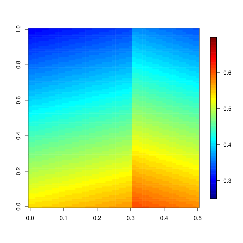
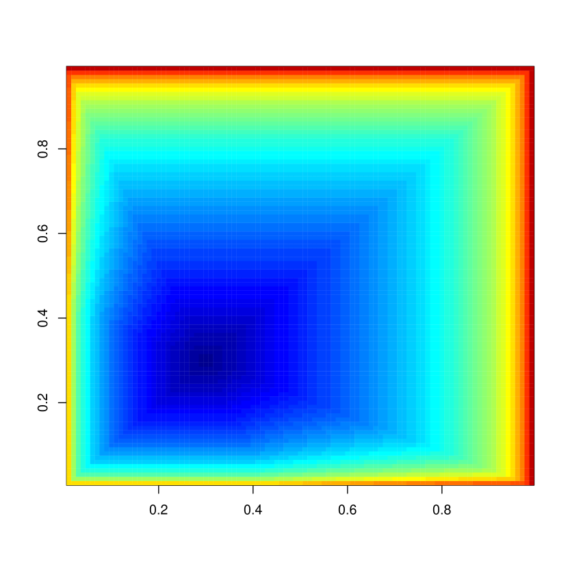
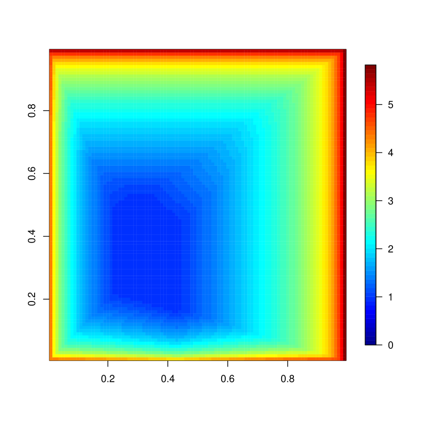
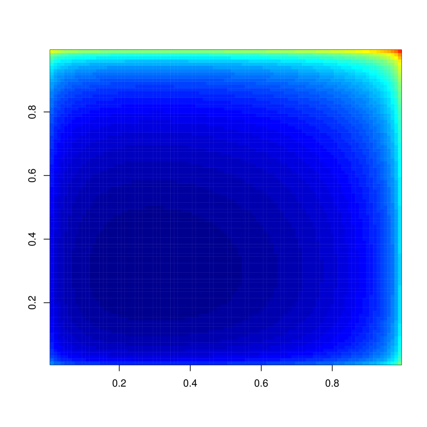
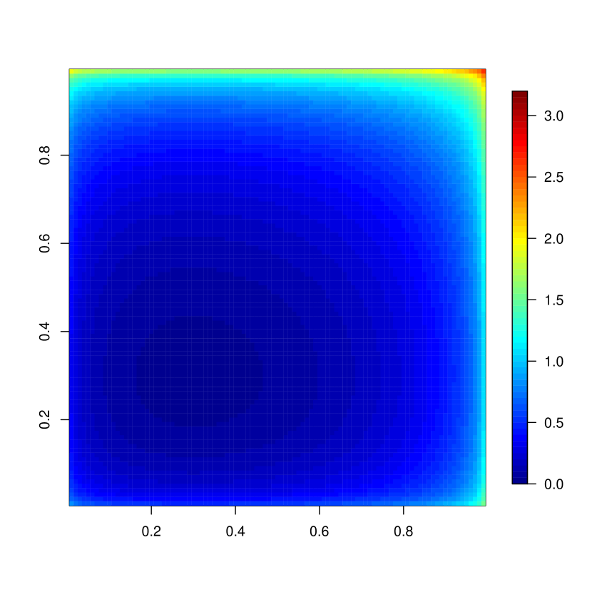
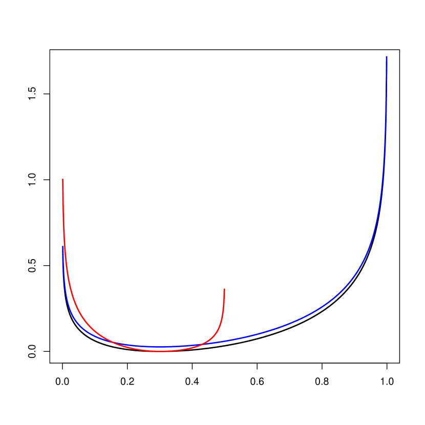
Suppose the context-specific model definition in Example 2 is completed by the probability specifications in Table 2. Suppose we are interested in the event that parents do not decide for vaccination. Figure 4 shows the sensitivity functions for this event when θ2111subscript𝜃subscript21subscript11\theta_{2_{1}1_{1}} (on the x-axis) and θ210subscript𝜃subscript210\theta_{21_{0}} (on the y-axis) are varied and the other covarying parameter are changed with different schemes. We can notice that for all schemes the functions are linear in their arguments and that more precisely for an order-preserving scheme the sensitivity function is piece-wise linear. Notice that whilst uniform and proportional covariation assigns similar, although different, probabilities to the event of interest, under order-preserving covariation the probability of interest changes very differently from the other schemes: a property we have often observed in our investigations.

Refer to caption
(a) Proportional.
Refer to caption
(b) Uniform.
Refer to caption
(c) Order-preserving.
Figure 4: Sensitivity functions for Example 4 under different covariation schemes.

4.3 The Chan-Darwiche distance

Whilst sensitivity functions study local changes, CD distances describe global variations in distributions [11]. These can be used to study by how much two vectors of atomic probabilities vary in their distributional assumptions if one arises from the other via a covariation scheme. We are then interested in the global impact of that local change.

We next characterize the form of the CD distance for multilinear models in single full CPT analyses, first generalizing its form, again derived in [45] for BN models. We demonstrate that the distance depends only on the varied and covaried parameters: thus very easy to compute.

Proposition 4.

Let 𝐩θ,𝐩θ~Ψsubscript𝐩𝜃subscript𝐩~𝜃subscriptΨ\bm{p}_{\theta},\bm{p}_{\tilde{\theta}}\in\mathbb{P}_{\Psi}, where ΨsubscriptΨ\mathbb{P}_{\Psi} is a multilinear parametric model and 𝐩θ~subscript𝐩~𝜃\bm{p}_{\tilde{\theta}} arises from 𝐩θsubscript𝐩𝜃\bm{p}_{\theta} by varying θjisubscript𝜃subscript𝑗𝑖\theta_{j_{i}} to θ~jisubscript~𝜃subscript𝑗𝑖\tilde{\theta}_{j_{i}} and θjsΘj{θji}subscript𝜃subscript𝑗𝑠subscriptΘ𝑗subscript𝜃subscript𝑗𝑖\theta_{j_{s}}\in\Theta_{j}\setminus\{\theta_{j_{i}}\} to θ~js=σj(θjs,θ~ji)subscript~𝜃subscript𝑗𝑠subscript𝜎𝑗subscript𝜃subscript𝑗𝑠subscript~𝜃subscript𝑗𝑖\tilde{\theta}_{j_{s}}=\sigma_{j}(\theta_{j_{s}},\tilde{\theta}_{j_{i}}), where σj(θjs,θ~ji)subscript𝜎𝑗subscript𝜃subscript𝑗𝑠subscript~𝜃subscript𝑗𝑖\sigma_{j}(\theta_{j_{s}},\tilde{\theta}_{j_{i}}) is a valid covariation scheme, j[n],s[rj]{ji}formulae-sequence𝑗delimited-[]𝑛𝑠delimited-[]subscript𝑟𝑗subscript𝑗𝑖j\in[n],s\in[r_{j}]\setminus\{j_{i}\}. Then the CD distance between 𝐩θsubscript𝐩𝜃\bm{p}_{\theta} and 𝐩θ~subscript𝐩~𝜃\bm{p}_{\tilde{\theta}} is equal to

𝒟CD(𝒑θ,𝒑θ~)=logmaxj[n]s[rj]θ~jsθjslogminj[n]s[rj]θ~jsθjs.subscript𝒟CDsubscript𝒑𝜃subscript𝒑~𝜃subscript𝑗delimited-[]𝑛𝑠delimited-[]subscript𝑟𝑗subscript~𝜃subscript𝑗𝑠subscript𝜃subscript𝑗𝑠subscript𝑗delimited-[]𝑛𝑠delimited-[]subscript𝑟𝑗subscript~𝜃subscript𝑗𝑠subscript𝜃subscript𝑗𝑠\mathcal{D}_{\textnormal{CD}}(\bm{p}_{\theta},\bm{p}_{\tilde{\theta}})=\log\max_{\begin{subarray}{c}j\in[n]\\ s\in[r_{j}]\end{subarray}}\frac{\tilde{\theta}_{j_{s}}}{\theta_{j_{s}}}-\log\min_{\begin{subarray}{c}j\in[n]\\ s\in[r_{j}]\end{subarray}}\frac{\tilde{\theta}_{j_{s}}}{\theta_{j_{s}}}. (11)
Proof.

For a multilinear parametric model the CD distance can be written as

𝒟CD(𝒑θ,𝒑θ~)subscript𝒟CDsubscript𝒑𝜃subscript𝒑~𝜃\displaystyle\mathcal{D}_{\textnormal{CD}}(\bm{p}_{\theta},\bm{p}_{\tilde{\theta}}) =logmax𝜶𝔸𝜽~𝜶𝜽𝜶logmin𝜶𝔸𝜽~𝜶𝜽𝜶absentsubscript𝜶𝔸superscript~𝜽𝜶superscript𝜽𝜶subscript𝜶𝔸superscript~𝜽𝜶superscript𝜽𝜶\displaystyle=\log\max_{\bm{\alpha}\in\mathbb{A}}\frac{\tilde{\bm{\theta}}^{\bm{\alpha}}}{\bm{\theta}^{\bm{\alpha}}}-\log\min_{\bm{\alpha}\in\mathbb{A}}\frac{\tilde{\bm{\theta}}^{\bm{\alpha}}}{\bm{\theta}^{\bm{\alpha}}}
=logmax{maxj[n]𝜶𝔸j𝜽~𝜶𝜽𝜶,max𝜶𝔸k[n]𝔸k𝜽~𝜶𝜽𝜶}logmin{minj[n]𝜶𝔸j𝜽~𝜶𝜽𝜶,min𝜶𝔸k[n]𝔸k𝜽~𝜶𝜽𝜶}.absentsubscript𝑗delimited-[]𝑛𝜶subscript𝔸𝑗superscript~𝜽𝜶superscript𝜽𝜶subscript𝜶limit-from𝔸subscript𝑘delimited-[]𝑛subscript𝔸𝑘superscript~𝜽𝜶superscript𝜽𝜶subscript𝑗delimited-[]𝑛𝜶subscript𝔸𝑗superscript~𝜽𝜶superscript𝜽𝜶subscript𝜶limit-from𝔸subscript𝑘delimited-[]𝑛subscript𝔸𝑘superscript~𝜽𝜶superscript𝜽𝜶\displaystyle=\log\max\left\{\max_{\begin{subarray}{c}j\in[n]\\ \bm{\alpha}\in\mathbb{A}_{j}\end{subarray}}\frac{\tilde{\bm{\theta}}^{\bm{\alpha}}}{\bm{\theta}^{\bm{\alpha}}},\max_{\bm{\alpha}\in\mathbb{A}\setminus\cup_{k\in[n]}\mathbb{A}_{k}}\frac{\tilde{\bm{\theta}}^{\bm{\alpha}}}{\bm{\theta}^{\bm{\alpha}}}\right\}-\log\min\left\{\min_{\begin{subarray}{c}j\in[n]\\ \bm{\alpha}\in\mathbb{A}_{j}\end{subarray}}\frac{\tilde{\bm{\theta}}^{\bm{\alpha}}}{\bm{\theta}^{\bm{\alpha}}},\min_{\bm{\alpha}\in\mathbb{A}\setminus\cup_{k\in[n]}\mathbb{A}_{k}}\frac{\tilde{\bm{\theta}}^{\bm{\alpha}}}{\bm{\theta}^{\bm{\alpha}}}\right\}.

If 𝜶𝔸k[n]𝔸k\bm{\alpha}\in\mathbb{A}\setminus\cup_{k\in[n]}\mathbb{A}_{k}, then 𝜽~=𝜽~𝜽𝜽\tilde{\bm{\theta}}=\bm{\theta} and thus 𝜽~𝜶/𝜽𝜶=1superscript~𝜽𝜶superscript𝜽𝜶1\tilde{\bm{\theta}}^{\bm{\alpha}}/\bm{\theta}^{\bm{\alpha}}=1. Because of the validity of the covariation scheme note that max𝜶𝔸j𝜽~𝜶/𝜽𝜶1subscript𝜶subscript𝔸𝑗superscript~𝜽𝜶superscript𝜽𝜶1\max_{\bm{\alpha}\in\mathbb{A}_{j}}\tilde{\bm{\theta}}^{\bm{\alpha}}/\bm{\theta}^{\bm{\alpha}}\geq 1 and min𝜶𝔸j𝜽~𝜶/𝜽𝜶1subscript𝜶subscript𝔸𝑗superscript~𝜽𝜶superscript𝜽𝜶1\min_{\bm{\alpha}\in\mathbb{A}_{j}}\tilde{\bm{\theta}}^{\bm{\alpha}}/\bm{\theta}^{\bm{\alpha}}\leq 1, for all j[n]𝑗delimited-[]𝑛j\in[n]. Thus

𝒟CD(𝒑θ,𝒑θ~)=logmaxj[n]𝜶𝔸j𝜽~𝜶𝜽𝜶logminj[n]𝜶𝔸j𝜽~𝜶𝜽𝜶.subscript𝒟CDsubscript𝒑𝜃subscript𝒑~𝜃subscript𝑗delimited-[]𝑛𝜶subscript𝔸𝑗superscript~𝜽𝜶superscript𝜽𝜶subscript𝑗delimited-[]𝑛𝜶subscript𝔸𝑗superscript~𝜽𝜶superscript𝜽𝜶\mathcal{D}_{\textnormal{CD}}(\bm{p}_{\theta},\bm{p}_{\tilde{\theta}})=\log\max_{\begin{subarray}{c}j\in[n]\\ \bm{\alpha}\in\mathbb{A}_{j}\end{subarray}}\frac{\tilde{\bm{\theta}}^{\bm{\alpha}}}{\bm{\theta}^{\bm{\alpha}}}-\log\min_{\begin{subarray}{c}j\in[n]\\ \bm{\alpha}\in\mathbb{A}_{j}\end{subarray}}\frac{\tilde{\bm{\theta}}^{\bm{\alpha}}}{\bm{\theta}^{\bm{\alpha}}}.

Now note that 𝜽~=𝜽jsθ~js~𝜽subscript𝜽subscript𝑗𝑠subscript~𝜃subscript𝑗𝑠\tilde{\bm{\theta}}=\bm{\theta}_{-j_{s}}\tilde{\theta}_{j_{s}}, for a θjsΘjsubscript𝜃subscript𝑗𝑠subscriptΘ𝑗\theta_{j_{s}}\in\Theta_{j}, j[n]𝑗delimited-[]𝑛j\in[n], since no two parameters in j[n]Θjsubscript𝑗delimited-[]𝑛subscriptΘ𝑗\cup_{j\in[n]}\Theta_{j} can have exponent non-zero in the same monomial. Thus 𝜽~𝜶/𝜽𝜶=θ~js/θjssuperscript~𝜽𝜶superscript𝜽𝜶subscript~𝜃subscript𝑗𝑠subscript𝜃subscript𝑗𝑠\tilde{\bm{\theta}}^{\bm{\alpha}}/\bm{\theta}^{\bm{\alpha}}=\tilde{\theta}_{j_{s}}/\theta_{j_{s}} since 𝜶{0,1}k𝜶superscript01𝑘\bm{\alpha}\in\{0,1\}^{k} and the result follows. ∎

We can now prove that the proportional covariation scheme is optimal for single full CPT analyses. This is important since a set of parameters might be varied to change an uncalibrated probability of interest, but a user might want to achieve this by choosing a distribution as close as possible to the original one. Several authors have posed this problem for BNs without finding a definitive answer [10, 45]. Here, exploiting our polynomial model representation, we can prove the optimality of the proportional scheme not only for BN models, but also for multilinear ones in single full CPT analyses.

Theorem 1.

Under the conditions of Proposition 4 and proportional covariations σj(θjs,θji)subscript𝜎𝑗subscript𝜃subscript𝑗𝑠subscript𝜃subscript𝑗𝑖\sigma_{j}(\theta_{j_{s}},\theta_{j_{i}}), the CD distance between 𝐩𝛉subscript𝐩𝛉\bm{p}_{\bm{\theta}} and 𝐩𝛉~subscript𝐩~𝛉\bm{p}_{\tilde{\bm{\theta}}} is minimized and can be written in closed form as

𝒟CD(𝒑θ,𝒑θ~)=logmaxj[n]{θ~jiθji,1θ~ji1θji}logminj[n]{θ~jiθji,1θ~ji1θji}.subscript𝒟CDsubscript𝒑𝜃subscript𝒑~𝜃subscript𝑗delimited-[]𝑛subscript~𝜃subscript𝑗𝑖subscript𝜃subscript𝑗𝑖1subscript~𝜃subscript𝑗𝑖1subscript𝜃subscript𝑗𝑖subscript𝑗delimited-[]𝑛subscript~𝜃subscript𝑗𝑖subscript𝜃subscript𝑗𝑖1subscript~𝜃subscript𝑗𝑖1subscript𝜃subscript𝑗𝑖\mathcal{D}_{\textnormal{CD}}(\bm{p}_{\theta},\bm{p}_{\tilde{\theta}})=\log\max_{j\in[n]}\left\{\frac{\tilde{\theta}_{j_{i}}}{\theta_{j_{i}}},\frac{1-\tilde{\theta}_{j_{i}}}{1-\theta_{j_{i}}}\right\}-\log\min_{j\in[n]}\left\{\frac{\tilde{\theta}_{j_{i}}}{\theta_{j_{i}}},\frac{1-\tilde{\theta}_{j_{i}}}{1-\theta_{j_{i}}}\right\}. (12)
Proof.

First note that we can write equation (11) as

𝒟CD(𝒑θ,𝒑θ~)=logmax{maxs[r1]θ~1sθ1s,,maxs[rn]θ~nsθns}logmin{mins[r1]θ~1sθ1s,,mins[rs]θ~nsθns}.subscript𝒟CDsubscript𝒑𝜃subscript𝒑~𝜃subscript𝑠delimited-[]subscript𝑟1subscript~𝜃subscript1𝑠subscript𝜃subscript1𝑠subscript𝑠delimited-[]subscript𝑟𝑛subscript~𝜃subscript𝑛𝑠subscript𝜃subscript𝑛𝑠subscript𝑠delimited-[]subscript𝑟1subscript~𝜃subscript1𝑠subscript𝜃subscript1𝑠subscript𝑠delimited-[]subscript𝑟𝑠subscript~𝜃subscript𝑛𝑠subscript𝜃subscript𝑛𝑠\mathcal{D}_{\textnormal{CD}}(\bm{p}_{\theta},\bm{p}_{\tilde{\theta}})=\log\max\left\{\max_{s\in[r_{1}]}\frac{\tilde{\theta}_{1_{s}}}{\theta_{1_{s}}},\dots,\max_{s\in[r_{n}]}\frac{\tilde{\theta}_{n_{s}}}{\theta_{n_{s}}}\right\}-\log\min\left\{\min_{s\in[r_{1}]}\frac{\tilde{\theta}_{1_{s}}}{\theta_{1_{s}}},\dots,\min_{s\in[r_{s}]}\frac{\tilde{\theta}_{n_{s}}}{\theta_{n_{s}}}\right\}. (13)

Now, let θ¯ji=θ~jisubscript¯𝜃subscript𝑗𝑖subscript~𝜃subscript𝑗𝑖\bar{\theta}_{j_{i}}=\tilde{\theta}_{j_{i}} and suppose θ¯jsΘj{θji}subscript¯𝜃subscript𝑗𝑠subscriptΘ𝑗subscript𝜃subscript𝑗𝑖\bar{\theta}_{j_{s}}\in\Theta_{j}\setminus\{\theta_{j_{i}}\} is obtained via a valid covariation scheme, j[n]𝑗delimited-[]𝑛j\in[n], s[rj]𝑠delimited-[]subscript𝑟𝑗s\in[r_{j}]. We want to prove that 𝒟CD(𝒑θ,𝒑θ¯)𝒟CD(𝒑θ,𝒑θ~)subscript𝒟CDsubscript𝒑𝜃subscript𝒑¯𝜃subscript𝒟CDsubscript𝒑𝜃subscript𝒑~𝜃\mathcal{D}_{\textnormal{CD}}(\bm{p}_{\theta},\bm{p}_{\bar{\theta}})\geq\mathcal{D}_{\textnormal{CD}}(\bm{p}_{\theta},\bm{p}_{\tilde{\theta}}). Suppose now the proportional scheme is optimal for one-way sensitivity analyses. If this is true, we must have that, for all j[n]𝑗delimited-[]𝑛j\in[n],

maxs[rj]θ¯jsθjsmaxs[rj]θ~jsθjs,andmins[rj]θ¯jsθjsmins[rj]θ~jsθjs.formulae-sequencesubscript𝑠delimited-[]subscript𝑟𝑗subscript¯𝜃subscript𝑗𝑠subscript𝜃subscript𝑗𝑠subscript𝑠delimited-[]subscript𝑟𝑗subscript~𝜃subscript𝑗𝑠subscript𝜃subscript𝑗𝑠andsubscript𝑠delimited-[]subscript𝑟𝑗subscript¯𝜃subscript𝑗𝑠subscript𝜃subscript𝑗𝑠subscript𝑠delimited-[]subscript𝑟𝑗subscript~𝜃subscript𝑗𝑠subscript𝜃subscript𝑗𝑠\max_{s\in[r_{j}]}\frac{\bar{\theta}_{j_{s}}}{\theta_{j_{s}}}\geq\max_{s\in[r_{j}]}\frac{\tilde{\theta}_{j_{s}}}{\theta_{j_{s}}},\hskip 28.45274pt\mbox{and}\hskip 28.45274pt\min_{s\in[r_{j}]}\frac{\bar{\theta}_{j_{s}}}{\theta_{j_{s}}}\leq\min_{s\in[r_{j}]}\frac{\tilde{\theta}_{j_{s}}}{\theta_{j_{s}}}.

Therefore,

max{maxs[r1]θ¯1sθ1s,,maxs[rn]θ¯nsθns}max{maxs[r1]θ~1sθ1s,,maxs[rn]θ~nsθns},subscript𝑠delimited-[]subscript𝑟1subscript¯𝜃subscript1𝑠subscript𝜃subscript1𝑠subscript𝑠delimited-[]subscript𝑟𝑛subscript¯𝜃subscript𝑛𝑠subscript𝜃subscript𝑛𝑠subscript𝑠delimited-[]subscript𝑟1subscript~𝜃subscript1𝑠subscript𝜃subscript1𝑠subscript𝑠delimited-[]subscript𝑟𝑛subscript~𝜃subscript𝑛𝑠subscript𝜃subscript𝑛𝑠\max\left\{\max_{s\in[r_{1}]}\frac{\bar{\theta}_{1_{s}}}{\theta_{1_{s}}},\dots,\max_{s\in[r_{n}]}\frac{\bar{\theta}_{n_{s}}}{\theta_{n_{s}}}\right\}\geq\max\left\{\max_{s\in[r_{1}]}\frac{\tilde{\theta}_{1_{s}}}{\theta_{1_{s}}},\dots,\max_{s\in[r_{n}]}\frac{\tilde{\theta}_{n_{s}}}{\theta_{n_{s}}}\right\},

and

min{mins[r1]θ¯1sθ1s,,mins[rn]θ¯nsθns}min{mins[r1]θ~1sθ1s,,mins[rn]θ~nsθns},subscript𝑠delimited-[]subscript𝑟1subscript¯𝜃subscript1𝑠subscript𝜃subscript1𝑠subscript𝑠delimited-[]subscript𝑟𝑛subscript¯𝜃subscript𝑛𝑠subscript𝜃subscript𝑛𝑠subscript𝑠delimited-[]subscript𝑟1subscript~𝜃subscript1𝑠subscript𝜃subscript1𝑠subscript𝑠delimited-[]subscript𝑟𝑛subscript~𝜃subscript𝑛𝑠subscript𝜃subscript𝑛𝑠\min\left\{\min_{s\in[r_{1}]}\frac{\bar{\theta}_{1_{s}}}{\theta_{1_{s}}},\dots,\min_{s\in[r_{n}]}\frac{\bar{\theta}_{n_{s}}}{\theta_{n_{s}}}\right\}\leq\min\left\{\min_{s\in[r_{1}]}\frac{\tilde{\theta}_{1_{s}}}{\theta_{1_{s}}},\dots,\min_{s\in[r_{n}]}\frac{\tilde{\theta}_{n_{s}}}{\theta_{n_{s}}}\right\},

from which the optimality condition follows.

We thus have to prove that for a single parameter change, the proportional covariation scheme minimizes the CD distance in any multilinear model. The proof follows similar steps to the one in [9] for BNs. Fix j[n]𝑗delimited-[]𝑛j\in[n] and note that if either θji=0subscript𝜃subscript𝑗𝑖0\theta_{j_{i}}=0 or θji=1subscript𝜃subscript𝑗𝑖1\theta_{j_{i}}=1 then the distance is infinite under both covariation schemes and the result holds. Consider now θji(0,1)subscript𝜃subscript𝑗𝑖01\theta_{j_{i}}\in(0,1) and suppose θ¯ji=θ~ji>θjisubscript¯𝜃subscript𝑗𝑖subscript~𝜃subscript𝑗𝑖subscript𝜃subscript𝑗𝑖\bar{\theta}_{j_{i}}=\tilde{\theta}_{j_{i}}>\theta_{j_{i}}. Under a proportional scheme, we have that

maxs[rj]θ~jsθjs=θ~jiθji and mins[rj]θ~jsθjs=θjs(1θ~ji)(θjs(1θji))=(1θ~ji)(1θji).subscript𝑠delimited-[]subscript𝑟𝑗subscript~𝜃subscript𝑗𝑠subscript𝜃subscript𝑗𝑠subscript~𝜃subscript𝑗𝑖subscript𝜃subscript𝑗𝑖 and subscript𝑠delimited-[]subscript𝑟𝑗subscript~𝜃subscript𝑗𝑠subscript𝜃subscript𝑗𝑠subscript𝜃subscript𝑗𝑠1subscript~𝜃subscript𝑗𝑖subscript𝜃subscript𝑗𝑠1subscript𝜃subscript𝑗𝑖1subscript~𝜃subscript𝑗𝑖1subscript𝜃subscript𝑗𝑖\max_{s\in[r_{j}]}\frac{\tilde{\theta}_{j_{s}}}{\theta_{j_{s}}}=\frac{\tilde{\theta}_{j_{i}}}{\theta_{j_{i}}}\,\,\,\,\mbox{ and }\,\,\,\,\min_{s\in[r_{j}]}\frac{\tilde{\theta}_{j_{s}}}{\theta_{j_{s}}}=\frac{\theta_{j_{s}}(1-\tilde{\theta}_{j_{i}})}{(\theta_{j_{s}}(1-\theta_{j_{i}}))}=\frac{(1-\tilde{\theta}_{j_{i}})}{(1-\theta_{j_{i}})}.

Conversely, for the generic covariation scheme σ(θjs,θ¯ji)𝜎subscript𝜃subscript𝑗𝑠subscript¯𝜃subscript𝑗𝑖\sigma(\theta_{j_{s}},\bar{\theta}_{j_{i}}) we have that

1θ¯ji1θji1subscript¯𝜃subscript𝑗𝑖1subscript𝜃subscript𝑗𝑖\displaystyle\frac{1-\bar{\theta}_{j_{i}}}{1-\theta_{j_{i}}} =s[rj]{ji}θ¯jss[rj]{ji}θjs=s[rj]{ji}θjs(θ¯js/θjs)s[rj]{ji}θjsabsentsubscript𝑠delimited-[]subscript𝑟𝑗subscript𝑗𝑖subscript¯𝜃subscript𝑗𝑠subscript𝑠delimited-[]subscript𝑟𝑗subscript𝑗𝑖subscript𝜃subscript𝑗𝑠subscript𝑠delimited-[]subscript𝑟𝑗subscript𝑗𝑖subscript𝜃subscript𝑗𝑠subscript¯𝜃subscript𝑗𝑠subscript𝜃subscript𝑗𝑠subscript𝑠delimited-[]subscript𝑟𝑗subscript𝑗𝑖subscript𝜃subscript𝑗𝑠\displaystyle=\frac{\sum_{s\in[r_{j}]\setminus\{j_{i}\}}\bar{\theta}_{j_{s}}}{\sum_{s\in[r_{j}]\setminus\{j_{i}\}}\theta_{j_{s}}}=\frac{\sum_{s\in[r_{j}]\setminus\{j_{i}\}}\theta_{j_{s}}(\bar{\theta}_{j_{s}}/\theta_{j_{s}})}{\sum_{s\in[r_{j}]\setminus\{j_{i}\}}\theta_{j_{s}}}
s[rj]{ji}θjs(mink[rj]θ¯k/θk)s[rj]{ji}θjs=mins[rj]θ¯sθs.absentsubscript𝑠delimited-[]subscript𝑟𝑗subscript𝑗𝑖subscript𝜃subscript𝑗𝑠subscript𝑘delimited-[]subscript𝑟𝑗subscript¯𝜃𝑘subscript𝜃𝑘subscript𝑠delimited-[]subscript𝑟𝑗subscript𝑗𝑖subscript𝜃subscript𝑗𝑠subscript𝑠delimited-[]subscript𝑟𝑗subscript¯𝜃𝑠subscript𝜃𝑠\displaystyle\geq\frac{\sum_{s\in[r_{j}]\setminus\{j_{i}\}}\theta_{j_{s}}(\min_{k\in[r_{j}]}\bar{\theta}_{k}/\theta_{k})}{\sum_{s\in[r_{j}]\setminus\{j_{i}\}}\theta_{j_{s}}}=\min_{s\in[r_{j}]}\frac{\bar{\theta}_{s}}{\theta_{s}}.

Thus since (1θ¯ji)/(1θji)=(1θ~ji)/(1θji)1subscript¯𝜃subscript𝑗𝑖1subscript𝜃subscript𝑗𝑖1subscript~𝜃subscript𝑗𝑖1subscript𝜃subscript𝑗𝑖(1-\bar{\theta}_{j_{i}})/(1-\theta_{j_{i}})=(1-\tilde{\theta}_{j_{i}})/(1-\theta_{j_{i}}) we have that mins[rj]θ~js/θjsmins[rj]θ¯js/θjssubscript𝑠delimited-[]subscript𝑟𝑗subscript~𝜃subscript𝑗𝑠subscript𝜃subscript𝑗𝑠subscript𝑠delimited-[]subscript𝑟𝑗subscript¯𝜃subscript𝑗𝑠subscript𝜃subscript𝑗𝑠\min_{s\in[r_{j}]}\tilde{\theta}_{j_{s}}/\theta_{j_{s}}\geq\min_{s\in[r_{j}]}\bar{\theta}_{j_{s}}/\theta_{j_{s}}. Furthermore,

maxs[rj]θ¯jsθjsθ¯jiθji=θ~jiθji=maxs[rj]θ~jsθjs.subscript𝑠delimited-[]subscript𝑟𝑗subscript¯𝜃subscript𝑗𝑠subscript𝜃subscript𝑗𝑠subscript¯𝜃subscript𝑗𝑖subscript𝜃subscript𝑗𝑖subscript~𝜃subscript𝑗𝑖subscript𝜃subscript𝑗𝑖subscript𝑠delimited-[]subscript𝑟𝑗subscript~𝜃subscript𝑗𝑠subscript𝜃subscript𝑗𝑠\max_{s\in[r_{j}]}\frac{\bar{\theta}_{j_{s}}}{\theta_{j_{s}}}\geq\frac{\bar{\theta}_{j_{i}}}{\theta_{j_{i}}}=\frac{\tilde{\theta}_{j_{i}}}{\theta_{j_{i}}}=\max_{s\in[r_{j}]}\frac{\tilde{\theta}_{j_{s}}}{\theta_{j_{s}}}.

It then follows that 𝒟CD(𝒑θ,𝒑θ¯)𝒟CD(𝒑θ,𝒑θ~)subscript𝒟CDsubscript𝒑𝜃subscript𝒑¯𝜃subscript𝒟CDsubscript𝒑𝜃subscript𝒑~𝜃\mathcal{D}_{\textnormal{CD}}(\bm{p}_{\theta},\bm{p}_{\bar{\theta}})\geq\mathcal{D}_{\textnormal{CD}}(\bm{p}_{\theta},\bm{p}_{\tilde{\theta}}) when θ~ji>θjisubscript~𝜃subscript𝑗𝑖subscript𝜃subscript𝑗𝑖\tilde{\theta}_{j_{i}}>\theta_{j_{i}} for one-way analyses. For the case θ~ji<θjisubscript~𝜃subscript𝑗𝑖subscript𝜃subscript𝑗𝑖\tilde{\theta}_{j_{i}}<\theta_{j_{i}} the proof mirrors the one presented here. The explicit form of the distance under a proportional covariation schemes in equation (12) follows by noting that the maximum and the minimum can either be θ~ji/θjisubscript~𝜃subscript𝑗𝑖subscript𝜃subscript𝑗𝑖\tilde{\theta}_{j_{i}}/\theta_{j_{i}} or (1θ~ji)/(1θji)1subscript~𝜃subscript𝑗𝑖1subscript𝜃subscript𝑗𝑖(1-\tilde{\theta}_{j_{i}})/(1-\theta_{j_{i}}). ∎

Example 5.
Refer to caption
(a) Proportional.
Refer to caption
(b) Uniform.
Refer to caption
(c) One-way analysis.
Figure 5: CD distances for Example 5 under different covariation schemes: proportional (black), uniform (blue), order-preserving (red).

In Figure 5 we plott the CD distance between the varied and the original probability distributions for Example 2 when θ2111subscript𝜃subscript21subscript11\theta_{2_{1}1_{1}} (x-axis) and θ210subscript𝜃subscript210\theta_{21_{0}} (y-axis in 5(a) and 5(b)) are varied for the covariation schemes so far considered. From Figures 5(a) and 5(b) we can get an intuition that the distance under proportional covariation is smaller than in the uniform case. This becomes clearer when we only let θ2111subscript𝜃subscript21subscript11\theta_{2_{1}1_{1}} vary as shown in Figure 5(c) since the black line is always underneath the others.

4.4 ϕitalic-ϕ\phi-divergences

Although the CD distance is widely used in sensitivity analyses, comparisons between two generic distributions are usually performed by computing the KL divergence. For one-way sensitivity analysis in BNs, the KL divergence equals the KL divergence between the original and varied conditional probability distribution of the manipulated parameter times the marginal probability of the conditioning parent configuration. This means that one way sensitivity analyses based on KL distances can become computationally infeasible, since this constant term might need to be computed an arbitrary large number of times. In Proposition 5 below we demonstrate that this property is common to any ϕitalic-ϕ\phi-divergence for any multilinear model and single full CPT analyses.

Proposition 5.

Let 𝐩θ,𝐩θ~Ψsubscript𝐩𝜃subscript𝐩~𝜃subscriptΨ\bm{p}_{\theta},\bm{p}_{\tilde{\theta}}\in\mathbb{P}_{\Psi}, where ΨsubscriptΨ\mathbb{P}_{\Psi} is a multilinear parametric model and 𝐩θ~subscript𝐩~𝜃\bm{p}_{\tilde{\theta}} arises from 𝐩θsubscript𝐩𝜃\bm{p}_{\theta} by varying θjisubscript𝜃subscript𝑗𝑖\theta_{j_{i}} to θ~jisubscript~𝜃subscript𝑗𝑖\tilde{\theta}_{j_{i}} and θjsΘj{θji}subscript𝜃subscript𝑗𝑠subscriptΘ𝑗subscript𝜃subscript𝑗𝑖\theta_{j_{s}}\in\Theta_{j}\setminus\{\theta_{j_{i}}\} to θ~js=σj(θjs,θ~ji)subscript~𝜃subscript𝑗𝑠subscript𝜎𝑗subscript𝜃subscript𝑗𝑠subscript~𝜃subscript𝑗𝑖\tilde{\theta}_{j_{s}}=\sigma_{j}(\theta_{j_{s}},\tilde{\theta}_{j_{i}}), where σj(θjs,θ~ji)subscript𝜎𝑗subscript𝜃subscript𝑗𝑠subscript~𝜃subscript𝑗𝑖\sigma_{j}(\theta_{j_{s}},\tilde{\theta}_{j_{i}}) is a valid covariation scheme, j[n],s[rj]{ji}formulae-sequence𝑗delimited-[]𝑛𝑠delimited-[]subscript𝑟𝑗subscript𝑗𝑖j\in[n],s\in[r_{j}]\setminus\{j_{i}\}. Then the ϕitalic-ϕ\phi-divergence between 𝐩θ~subscript𝐩~𝜃\bm{p}_{\tilde{\theta}} and 𝐩θsubscript𝐩𝜃\bm{p}_{\theta} is equal to

𝒟ϕ(𝒑θ~,𝒑θ)=j[n]𝒟ϕ(𝒑θ~j,𝒑θj)s[rj]𝜶𝔸js𝜽js𝜶,subscript𝒟italic-ϕsubscript𝒑~𝜃subscript𝒑𝜃subscript𝑗delimited-[]𝑛subscript𝒟italic-ϕsubscriptsuperscript𝒑𝑗~𝜃subscriptsuperscript𝒑𝑗𝜃subscript𝑠delimited-[]subscript𝑟𝑗subscript𝜶subscript𝔸subscript𝑗𝑠superscriptsubscript𝜽subscript𝑗𝑠𝜶\mathcal{D}_{\phi}(\bm{p}_{\tilde{\theta}},\bm{p}_{\theta})=\sum_{j\in[n]}\mathcal{D}_{\phi}(\bm{p}^{j}_{\tilde{\theta}},\bm{p}^{j}_{\theta})\sum_{s\in[r_{j}]}\sum_{\bm{\alpha}\in\mathbb{A}_{-j_{s}}}\bm{\theta}_{-j_{s}}^{\bm{\alpha}}, (14)

where 𝐩θjsubscriptsuperscript𝐩𝑗𝜃\bm{p}^{j}_{\theta} denotes the vector of atomic probabilities in ΘjsubscriptΘ𝑗\Theta_{j}.

Proof.

For a model with monomial parametrisation the ϕitalic-ϕ\phi-divergence can be written as

𝒟ϕ(𝒑θ~,𝒑θ)subscript𝒟italic-ϕsubscript𝒑~𝜃subscript𝒑𝜃\displaystyle\mathcal{D}_{\phi}(\bm{p}_{\tilde{\theta}},\bm{p}_{\theta}) =𝜶𝔸𝜽𝜶ϕ(𝜽~𝜶𝜽𝜶)=j[n]𝜶𝔸j𝜽𝜶ϕ(𝜽~𝜶𝜽𝜶)+𝜶𝔸j[n]𝔸j𝜽𝜶ϕ(𝜽~𝜶𝜽𝜶).absentsubscript𝜶𝔸superscript𝜽𝜶italic-ϕsuperscript~𝜽𝜶superscript𝜽𝜶subscript𝑗delimited-[]𝑛subscript𝜶subscript𝔸𝑗superscript𝜽𝜶italic-ϕsuperscript~𝜽𝜶superscript𝜽𝜶subscript𝜶limit-from𝔸subscript𝑗delimited-[]𝑛subscript𝔸𝑗superscript𝜽𝜶italic-ϕsuperscript~𝜽𝜶superscript𝜽𝜶\displaystyle=\sum_{\bm{\alpha}\in\mathbb{A}}\bm{\theta}^{\bm{\alpha}}\phi\left(\frac{\tilde{\bm{\theta}}^{\bm{\alpha}}}{\bm{\theta}^{\bm{\alpha}}}\right)=\sum_{j\in[n]}\sum_{\bm{\alpha}\in\mathbb{A}_{j}}\bm{\theta}^{\bm{\alpha}}\phi\left(\frac{\tilde{\bm{\theta}}^{\bm{\alpha}}}{\bm{\theta}^{\bm{\alpha}}}\right)+\sum_{\bm{\alpha}\in\mathbb{A}\setminus\cup_{j\in[n]}\mathbb{A}_{j}}\bm{\theta}^{\bm{\alpha}}\phi\left(\frac{\tilde{\bm{\theta}}^{\bm{\alpha}}}{\bm{\theta}^{\bm{\alpha}}}\right).

Notice that for 𝜶𝔸j[n]𝔸j\bm{\alpha}\in\mathbb{A}\setminus\cup_{j\in[n]}\mathbb{A}_{j}, 𝜽~𝜶/𝜽𝜶=1superscript~𝜽𝜶superscript𝜽𝜶1\tilde{\bm{\theta}}^{\bm{\alpha}}/\bm{\theta}^{\bm{\alpha}}=1. Thus, since ϕ(1)=0italic-ϕ10\phi(1)=0, we then have that

𝒟ϕ(𝒑θ~,𝒑θ)subscript𝒟italic-ϕsubscript𝒑~𝜃subscript𝒑𝜃\displaystyle\mathcal{D}_{\phi}(\bm{p}_{\tilde{\theta}},\bm{p}_{\theta}) =j[n]𝜶𝔸j𝜽𝜶ϕ(𝜽~𝜶𝜽𝜶)=j[n]s[rj]𝜶𝔸js𝜽js𝜶θjsϕ(𝜽js𝜶θ~js𝜽js𝜶θjs)absentsubscript𝑗delimited-[]𝑛subscript𝜶subscript𝔸𝑗superscript𝜽𝜶italic-ϕsuperscript~𝜽𝜶superscript𝜽𝜶subscript𝑗delimited-[]𝑛subscript𝑠delimited-[]subscript𝑟𝑗subscript𝜶subscript𝔸subscript𝑗𝑠superscriptsubscript𝜽subscript𝑗𝑠𝜶subscript𝜃subscript𝑗𝑠italic-ϕsuperscriptsubscript𝜽subscript𝑗𝑠𝜶subscript~𝜃subscript𝑗𝑠superscriptsubscript𝜽subscript𝑗𝑠𝜶subscript𝜃subscript𝑗𝑠\displaystyle=\sum_{j\in[n]}\sum_{\bm{\alpha}\in\mathbb{A}_{j}}\bm{\theta}^{\bm{\alpha}}\phi\left(\frac{\tilde{\bm{\theta}}^{\bm{\alpha}}}{\bm{\theta}^{\bm{\alpha}}}\right)=\sum_{j\in[n]}\sum_{s\in[r_{j}]}\sum_{\bm{\alpha}\in\mathbb{A}_{-j_{s}}}\bm{\theta}_{-j_{s}}^{\bm{\alpha}}\theta_{j_{s}}\phi\left(\frac{\bm{\theta}_{-j_{s}}^{\bm{\alpha}}\tilde{\theta}_{j_{s}}}{\bm{\theta}_{-j_{s}}^{\bm{\alpha}}\theta_{j_{s}}}\right)
=j[n]s[rj]θjsϕ(θ~jsθjs)𝜶𝔸js𝜽js𝜶=j[n]𝒟ϕ(𝒑θ~j,𝒑θj)s[rj]𝜶𝔸js𝜽js𝜶.absentsubscript𝑗delimited-[]𝑛subscript𝑠delimited-[]subscript𝑟𝑗subscript𝜃subscript𝑗𝑠italic-ϕsubscript~𝜃subscript𝑗𝑠subscript𝜃subscript𝑗𝑠subscript𝜶subscript𝔸subscript𝑗𝑠superscriptsubscript𝜽subscript𝑗𝑠𝜶subscript𝑗delimited-[]𝑛subscript𝒟italic-ϕsubscriptsuperscript𝒑𝑗~𝜃subscriptsuperscript𝒑𝑗𝜃subscript𝑠delimited-[]subscript𝑟𝑗subscript𝜶subscript𝔸subscript𝑗𝑠superscriptsubscript𝜽subscript𝑗𝑠𝜶\displaystyle=\sum_{j\in[n]}\sum_{s\in[r_{j}]}\theta_{j_{s}}\phi\left(\frac{\tilde{\theta}_{j_{s}}}{\theta_{j_{s}}}\right)\sum_{\bm{\alpha}\in\mathbb{A}_{-j_{s}}}\bm{\theta}_{-j_{s}}^{\bm{\alpha}}=\sum_{j\in[n]}\mathcal{D}_{\phi}(\bm{p}^{j}_{\tilde{\theta}},\bm{p}^{j}_{\theta})\sum_{s\in[r_{j}]}\sum_{\bm{\alpha}\in\mathbb{A}_{-j_{s}}}\bm{\theta}_{-j_{s}}^{\bm{\alpha}}.

The additional complexity of having to compute the constant term in equation (14) has limited the use of KL divergences, and more generally ϕitalic-ϕ\phi-divergences, in both practical and theoretical sensitivity investigations in discrete BNs. However, looking at probabilistic models from a polynomial point of view, we are able here to establish an additional strong theoretical justification for the use proportional covariation even in single full CPT analyses, since this also minimizes any ϕitalic-ϕ\phi-divergence.

Theorem 2.

Under the conditions of Proposition 5, 𝒟ϕ(𝐩θ~,𝐩θ)subscript𝒟italic-ϕsubscript𝐩~𝜃subscript𝐩𝜃\mathcal{D}_{\phi}(\bm{p}_{\tilde{\theta}},\bm{p}_{\theta}) is minimized by the proportional covariation schemes σj(θjs,θ~ji)=(1θ~ji)θjs/(1θji)subscript𝜎𝑗subscript𝜃subscript𝑗𝑠subscript~𝜃subscript𝑗𝑖1subscript~𝜃subscript𝑗𝑖subscript𝜃subscript𝑗𝑠1subscript𝜃subscript𝑗𝑖\sigma_{j}(\theta_{j_{s}},\tilde{\theta}_{j_{i}})=(1-\tilde{\theta}_{j_{i}})\theta_{j_{s}}/(1-\theta_{j_{i}}).

Proof.

Since s[rj]𝜶𝔸js𝜽js𝜶subscript𝑠delimited-[]subscript𝑟𝑗subscript𝜶subscript𝔸subscript𝑗𝑠superscriptsubscript𝜽subscript𝑗𝑠𝜶\sum_{s\in[r_{j}]}\sum_{\bm{\alpha}\in\mathbb{A}_{-j_{s}}}\bm{\theta}_{-j_{s}}^{\bm{\alpha}} in equation (14) is a positive constant, 𝒟ϕ(𝒑θ~,𝒑θ)subscript𝒟italic-ϕsubscript𝒑~𝜃subscript𝒑𝜃\mathcal{D}_{\phi}(\bm{p}_{\tilde{\theta}},\bm{p}_{\theta}) is minimized if each 𝒟ϕ(𝒑θ~j,𝒑θj)subscript𝒟italic-ϕsubscriptsuperscript𝒑𝑗~𝜃subscriptsuperscript𝒑𝑗𝜃\mathcal{D}_{\phi}(\bm{p}^{j}_{\tilde{\theta}},\bm{p}^{j}_{\theta}) attains its minimum. Fix a j[n]𝑗delimited-[]𝑛j\in[n]. We use the method of Lagrange multipliers to demonstrate that 𝒟ϕ(𝒑θ~j,𝒑θj)subscript𝒟italic-ϕsubscriptsuperscript𝒑𝑗~𝜃subscriptsuperscript𝒑𝑗𝜃\mathcal{D}_{\phi}(\bm{p}^{j}_{\tilde{\theta}},\bm{p}^{j}_{\theta}) is minimized by proportional covariation, subject to the constraint that s[rj]θ~js1=0subscript𝑠delimited-[]subscript𝑟𝑗subscript~𝜃subscript𝑗𝑠10\sum_{s\in[r_{j}]}\tilde{\theta}_{j_{s}}-1=0. Define

L=s[rj]θjsϕ(θ~jsθjs)λ(s[rj]θ~js1).𝐿subscript𝑠delimited-[]subscript𝑟𝑗subscript𝜃subscript𝑗𝑠italic-ϕsubscript~𝜃subscript𝑗𝑠subscript𝜃subscript𝑗𝑠𝜆subscript𝑠delimited-[]subscript𝑟𝑗subscript~𝜃subscript𝑗𝑠1L=\sum_{s\in[r_{j}]}\theta_{j_{s}}\phi\left(\frac{\tilde{\theta}_{j_{s}}}{\theta_{j_{s}}}\right)-\lambda\left(\sum_{s\in[r_{j}]}\tilde{\theta}_{j_{s}}-1\right).

Taking the first derivative of L𝐿L with respect to θ~jssubscript~𝜃subscript𝑗𝑠\tilde{\theta}_{j_{s}} and equating it to zero gives

θ~jsL=ϕ(θ~jsθjs)=λ,subscript~𝜃subscript𝑗𝑠𝐿superscriptitalic-ϕsubscript~𝜃subscript𝑗𝑠subscript𝜃subscript𝑗𝑠𝜆\frac{\partial}{\partial\tilde{\theta}_{j_{s}}}L=\phi^{\prime}\left(\frac{\tilde{\theta}_{j_{s}}}{\theta_{j_{s}}}\right)=\lambda,

where ϕsuperscriptitalic-ϕ\phi^{\prime} denotes the derivative of ϕitalic-ϕ\phi. By inverting we then deduce that

θ~js=ϕ(λ)1θjs.subscript~𝜃subscript𝑗𝑠superscriptitalic-ϕsuperscript𝜆1subscript𝜃subscript𝑗𝑠\tilde{\theta}_{j_{s}}=\phi^{\prime}(\lambda)^{-1}\theta_{j_{s}}. (15)

Since equation (15) holds for every s[rj]{ji}𝑠delimited-[]subscript𝑟𝑗subscript𝑗𝑖s\in[r_{j}]\setminus\{j_{i}\} we have that

s[rj]{ji}θ~js=ϕ(λ)1s[rj]{ji}θjssubscript𝑠delimited-[]subscript𝑟𝑗subscript𝑗𝑖subscript~𝜃subscript𝑗𝑠superscriptitalic-ϕsuperscript𝜆1subscript𝑠delimited-[]subscript𝑟𝑗subscript𝑗𝑖subscript𝜃subscript𝑗𝑠\sum_{s\in[r_{j}]\setminus\{j_{i}\}}\tilde{\theta}_{j_{s}}=\phi^{\prime}(\lambda)^{-1}\sum_{s\in[r_{j}]\setminus\{j_{i}\}}\theta_{j_{s}} (16)

Now take the first partial derivative of L𝐿L with respect to λ𝜆\lambda and equate it to zero. This gives

λL=s[rj]θ~js=1s[rj]{ji}θ~js=1θ~jiformulae-sequence𝜆𝐿subscript𝑠delimited-[]subscript𝑟𝑗subscript~𝜃subscript𝑗𝑠1subscript𝑠delimited-[]subscript𝑟𝑗subscript𝑗𝑖subscript~𝜃subscript𝑗𝑠1subscript~𝜃subscript𝑗𝑖\frac{\partial}{\partial\lambda}L=\sum_{s\in[r_{j}]}\tilde{\theta}_{j_{s}}=1\ \ \ \ \Longrightarrow\ \ \ \ \sum_{s\in[r_{j}]\setminus\{j_{i}\}}\tilde{\theta}_{j_{s}}=1-\tilde{\theta}_{j_{i}} (17)

Plugging the right hand side of (17) into (16), we deduce that

ϕ(λ)1=1θ~jis[rj]{ji}θjs=1θ~ji1θji.superscriptitalic-ϕsuperscript𝜆11subscript~𝜃subscript𝑗𝑖subscript𝑠delimited-[]subscript𝑟𝑗subscript𝑗𝑖subscript𝜃subscript𝑗𝑠1subscript~𝜃subscript𝑗𝑖1subscript𝜃subscript𝑗𝑖\phi^{\prime}(\lambda)^{-1}=\frac{1-\tilde{\theta}_{j_{i}}}{\sum_{s\in[r_{j}]\setminus\{j_{i}\}}\theta_{j_{s}}}=\frac{1-\tilde{\theta}_{j_{i}}}{1-\theta_{j_{i}}}. (18)

Thus, by plugging (18) into (15) we conclude that

θ~js=1θ~ji1θjiθjs.subscript~𝜃subscript𝑗𝑠1subscript~𝜃subscript𝑗𝑖1subscript𝜃subscript𝑗𝑖subscript𝜃subscript𝑗𝑠\tilde{\theta}_{j_{s}}=\frac{1-\tilde{\theta}_{j_{i}}}{1-\theta_{j_{i}}}\theta_{j_{s}}.

This is guaranteed to be a minimum by the convexity of the function ϕitalic-ϕ\phi. ∎

Example 6.
Refer to caption
(a) Proportional.
Refer to caption
(b) Uniform.
Refer to caption
(c) One-way analysis.
Figure 6: KL divergences for Example 6 under different covariation schemes: proportional (black), uniform (blue), order-preserving (red).

As an example of a ϕitalic-ϕ\phi-divergence, in Figure 6 we plot KL(𝐩θ,𝐩θ~)subscript𝐩𝜃subscript𝐩~𝜃(\bm{p}_{\theta},\bm{p}_{\tilde{\theta}}) for Example 2 when θ2111subscript𝜃subscript21subscript11\theta_{2_{1}1_{1}} (x-axis) and θ210subscript𝜃subscript210\theta_{21_{0}} (y-axis in 6(a) and 6(b)) are varied for the covariation schemes so far considered. From Figures 6(a) and 6(b) we can get an intuition that the KL divergence under proportional covariation is smaller than in the uniform case. This becomes clearer when we only let θ2111subscript𝜃subscript21subscript11\theta_{2_{1}1_{1}} vary as shown in Figure 6(c) since the black line is always underneath the others.

5 One-way sensitivity analysis in non-multilinear models

For multilinear models we have been able to provide a unifying framework to perform various sensitivity analyses by deducing closed forms for both sensitivity functions and various divergences. Unfortunately, this is not possible for non-multilinear parametric models because these will depend on the degree of both the indeterminate to be varied and the covaried parameters, which is not necessarily equal to one. However, representing the model through its interpolating polynomial will enable us to study central properties of various sensitivity analyses. Since sensitivity functions and CD distances are most commonly applied, in this section we will only focus on these. Furthermore, because of the much more general structure underlying non-multilinear models, we will restrict our discussion to one-way sensitivity methods. As in Section 4.1, we let θiΘCsubscript𝜃𝑖subscriptΘ𝐶\theta_{i}\in\Theta_{C} be varied to θ~isubscript~𝜃𝑖\tilde{\theta}_{i}, where ΘC={θj:j[r]}subscriptΘ𝐶conditional-setsubscript𝜃𝑗𝑗delimited-[]𝑟\Theta_{C}=\{\theta_{j}:j\in[r]\} is the set of parameters including θisubscript𝜃𝑖\theta_{i} which need to respect the sum-to-one condition.

5.1 Sensitivity functions

As in Section 4 we let f𝒚Tsubscript𝑓subscript𝒚𝑇f_{\bm{y}_{T}} denote a sensitivity function and f𝒚T𝒚Osuperscriptsubscript𝑓subscript𝒚𝑇subscript𝒚𝑂f_{\bm{y}_{T}}^{\bm{y}_{O}} a posterior sensitivity function.

Proposition 6.

Consider a parametric model ΨsubscriptΨ\mathbb{P}_{\Psi} with monomial parametrisation ΨΨ\Psi. Let θisubscript𝜃𝑖\theta_{i} vary to θ~isubscript~𝜃𝑖\tilde{\theta}_{i} and θjΘC{θi}subscript𝜃𝑗subscriptΘ𝐶subscript𝜃𝑖\theta_{j}\in\Theta_{C}\setminus\{\theta_{i}\} covary according to a linear scheme. The sensitivity function f𝐲T(θ~i)subscript𝑓subscript𝐲𝑇subscript~𝜃𝑖f_{\bm{y}_{T}}(\tilde{\theta}_{i}) is then a polynomial with degree lower or equal to d𝑑d, where d=max𝛂𝕋C,j[r]{αj}𝑑subscriptformulae-sequence𝛂subscript𝕋𝐶𝑗delimited-[]𝑟subscript𝛼𝑗d=\max_{\bm{\alpha}\in\mathbb{T}_{C},j\in[r]}\{\alpha_{j}\}. The posterior sensitivity function f𝐲T𝐲O(θ~i)superscriptsubscript𝑓subscript𝐲𝑇subscript𝐲𝑂subscript~𝜃𝑖f_{\bm{y}_{T}}^{\bm{y}_{O}}(\tilde{\theta}_{i}) is a rational function whose numerator and denominator are polynomials again with degree lower or equal to d𝑑d.

Proof.

This follows by noting that under the conditions of the proposition an exponent αi,𝒚subscript𝛼𝑖𝒚\alpha_{i,\bm{y}} in Definition 3 of monomial parametrisation, for any 𝜶𝒚𝔸subscript𝜶𝒚𝔸\bm{\alpha}_{\bm{y}}\in\mathbb{A} cannot be larger than d𝑑d. ∎

Similar results to Proposition 6 were presented in [13, 14, 44] for some specific classes of DBNs only.

The specific form of the sensitivity function in non-multilinear models depends both on the form of the interpolating polynomial, on the parameter to be varied and on the parameters that are consequently covaried. Therefore it is not possible to deduce a unique closed form expression since this will explicitly depend on the degree of all the above indeterminates. However, the interpolating polynomial enables us to identify a straightforward procedure to compute f𝒚T(θ~i)subscript𝑓subscript𝒚𝑇subscript~𝜃𝑖f_{\bm{y}_{T}}(\tilde{\theta}_{i}) as follows:

  1. 1.

    determine the polynomial cΨ(θ,𝒚T)subscript𝑐subscriptΨ𝜃subscript𝒚𝑇c_{\mathbb{P}_{\Psi}}(\theta,\bm{y}_{T}) for an event 𝕐Tsubscript𝕐𝑇\mathbb{Y}_{T};

  2. 2.

    replace θisubscript𝜃𝑖\theta_{i} by θ~isubscript~𝜃𝑖\tilde{\theta}_{i};

  3. 3.

    replace θjsubscript𝜃𝑗\theta_{j} by σ(θj,θ~i)𝜎subscript𝜃𝑗subscript~𝜃𝑖\sigma(\theta_{j},\tilde{\theta}_{i}) for θjΘC{θi}subscript𝜃𝑗subscriptΘ𝐶subscript𝜃𝑖\theta_{j}\in\Theta_{C}\setminus\{\theta_{i}\}.

θ^1120=0.4,subscript^𝜃subscript11subscript200.4\hat{\theta}_{1_{1}2_{0}}=0.4, θ^1121=0.6,subscript^𝜃subscript11subscript210.6\hat{\theta}_{1_{1}2_{1}}=0.6, θ^1122=0.7,subscript^𝜃subscript11subscript220.7\hat{\theta}_{1_{1}2_{2}}=0.7, θ^3020=0.9,subscript^𝜃subscript30subscript200.9\hat{\theta}_{3_{0}2_{0}}=0.9, θ^3021=0.6,subscript^𝜃subscript30subscript210.6\hat{\theta}_{3_{0}2_{1}}=0.6, θ^3022=0.2,subscript^𝜃subscript30subscript220.2\hat{\theta}_{3_{0}2_{2}}=0.2,
θ^212030=0.3,subscript^𝜃subscript21subscript20subscript300.3\hat{\theta}_{2_{1}2_{0}3_{0}}=0.3, θ^222030=0.2subscript^𝜃subscript22subscript20subscript300.2\hat{\theta}_{2_{2}2_{0}3_{0}}=0.2 θ^212130=0.3subscript^𝜃subscript21subscript21subscript300.3\hat{\theta}_{2_{1}2_{1}3_{0}}=0.3 θ^222130=0.5subscript^𝜃subscript22subscript21subscript300.5\hat{\theta}_{2_{2}2_{1}3_{0}}=0.5 θ^212230=0.5subscript^𝜃subscript21subscript22subscript300.5\hat{\theta}_{2_{1}2_{2}3_{0}}=0.5 θ^222230=0.3subscript^𝜃subscript22subscript22subscript300.3\hat{\theta}_{2_{2}2_{2}3_{0}}=0.3.
Table 3: Probability specifications for Example 7.
Refer to caption
Figure 7: Sensitivity functions in Example 7 when θ^212130subscript^𝜃subscript21subscript21subscript30\hat{\theta}_{2_{1}2_{1}3_{0}} (on the x-axis) is varied: proportional (black), uniform (blue) and order-preserving (red).
Example 7.

Suppose the definition of the DBN model in Example 3 is embellished by the probability specifications in Table 3. Suppose further the first time point distribution coincides with one defined in Table 1 for the context-specific BN in Example 2. We are now interested in the event (Y1(t)=1,Y2(1)=1,Y2(4)=1,Y3(t)=0,t[4])formulae-sequencesubscript𝑌1𝑡1formulae-sequencesubscript𝑌211formulae-sequencesubscript𝑌241formulae-sequencesubscript𝑌3𝑡0𝑡delimited-[]4(Y_{1}(t)=1,Y_{2}(1)=1,Y_{2}(4)=1,Y_{3}(t)=0,t\in[4]). By applying the above procedure to the interpolating polynomial of this DBN we can deduce that the sensitivity function when θ^212130subscript^𝜃subscript21subscript21subscript30\hat{\theta}_{2_{1}2_{1}3_{0}} is varied to x𝑥x equals

ax3+bxσ(θ^202130,x)+cxσ(θ^222130,x)+dσ(θ^202130,x)+eσ(θ^222130,x),𝑎superscript𝑥3𝑏𝑥𝜎subscript^𝜃subscript20subscript21subscript30𝑥𝑐𝑥𝜎subscript^𝜃subscript22subscript21subscript30𝑥𝑑𝜎subscript^𝜃subscript20subscript21subscript30𝑥𝑒𝜎subscript^𝜃subscript22subscript21subscript30𝑥ax^{3}+bx\sigma(\hat{\theta}_{2_{0}2_{1}3_{0}},x)+cx\sigma(\hat{\theta}_{2_{2}2_{1}3_{0}},x)+d\sigma(\hat{\theta}_{2_{0}2_{1}3_{0}},x)+e\sigma(\hat{\theta}_{2_{2}2_{1}3_{0}},x),

where a,b,c,d,e[0,1]𝑎𝑏𝑐𝑑𝑒01a,b,c,d,e\in[0,1]. This is plotted in Figure 7 for different covariation schemes. As formalized in Proposition 6 these are not linear in their arguments, but more generally polynomial. As in the multilinear case, we can notice that the probability of interest under order-preserving covariation behaves rather differently than under uniform and proportional covariation.

5.2 CD distance

We next introduce a general procedure to compute the CD distance for parametric models with monomial parametrisation.

Proposition 7.

Let 𝐩θ,𝐩θ~Ψsubscript𝐩𝜃subscript𝐩~𝜃subscriptΨ\bm{p}_{\theta},\bm{p}_{\tilde{\theta}}\in\mathbb{P}_{\Psi}, where ΨsubscriptΨ\mathbb{P}_{\Psi} is a parametric model with monomial parametrisation. The CD distance between 𝐩θsubscript𝐩𝜃\bm{p}_{\theta} and 𝐩θ~subscript𝐩~𝜃\bm{p}_{\tilde{\theta}} when θisubscript𝜃𝑖\theta_{i} is varied to θ~isubscript~𝜃𝑖\tilde{\theta}_{i} and θjΘC{θi}subscript𝜃𝑗subscriptΘ𝐶subscript𝜃𝑖\theta_{j}\in\Theta_{C}\setminus\{\theta_{i}\} is covaried to θ~j=σ(θj,θ~i)subscript~𝜃𝑗𝜎subscript𝜃𝑗subscript~𝜃𝑖\tilde{\theta}_{j}=\sigma(\theta_{j},\tilde{\theta}_{i}), j[r]{i}𝑗delimited-[]𝑟𝑖j\in[r]\setminus\{i\}, according to a valid covariation scheme can be computed from the interpolating polynomial as follows:

  1. 1.

    set 𝜽𝜶=0superscript𝜽𝜶0\bm{\theta}^{\bm{\alpha}}=0 for all 𝜶𝔸𝔸C𝜶𝔸subscript𝔸𝐶\bm{\alpha}\in\mathbb{A}\setminus\mathbb{A}_{C};

  2. 2.

    set θk=1subscript𝜃𝑘1\theta_{k}=1, if k[r]𝑘delimited-[]𝑟k\not\in[r], in any monomial 𝜽𝜶superscript𝜽𝜶\bm{\theta}^{\bm{\alpha}}, 𝜶𝔸C𝜶subscript𝔸𝐶\bm{\alpha}\in\mathbb{A}_{C};

  3. 3.

    call ΦΦ\Phi the set of remaining monomials, ϕ𝜶superscriptbold-italic-ϕ𝜶\bm{\phi}^{\bm{\alpha}} a generic element of ΦΦ\Phi and ϕ~𝜶superscript~bold-italic-ϕ𝜶\tilde{\bm{\phi}}^{\bm{\alpha}} its varied version;

  4. 4.

    set u=maxΦϕ~𝜶/ϕ𝜶𝑢subscriptΦsuperscript~bold-italic-ϕ𝜶superscriptbold-italic-ϕ𝜶u=\max_{\Phi}\tilde{\bm{\phi}}^{\bm{\alpha}}/\bm{\phi}^{\bm{\alpha}} and l=minΦϕ~𝜶/ϕ𝜶𝑙subscriptΦsuperscript~bold-italic-ϕ𝜶superscriptbold-italic-ϕ𝜶l=\min_{\Phi}\tilde{\bm{\phi}}^{\bm{\alpha}}/\bm{\phi}^{\bm{\alpha}};

  5. 5.

    compute CD(𝒑θ,𝒑θ~)=log(u)log(l)CDsubscript𝒑𝜃subscript𝒑~𝜃𝑢𝑙\textnormal{CD}(\bm{p}_{\theta},\bm{p}_{\tilde{\theta}})=\log(u)-\log(l).

It then follows that CD(𝐩θ,𝐩θ~)=CD(𝐩ϕ,𝐩ϕ~)CDsubscript𝐩𝜃subscript𝐩~𝜃CDsubscript𝐩italic-ϕsubscript𝐩~italic-ϕ\textnormal{CD}(\bm{p}_{\theta},\bm{p}_{\tilde{\theta}})=\textnormal{CD}(\bm{p}_{\phi},\bm{p}_{\tilde{\phi}}), where 𝐩ϕsubscript𝐩italic-ϕ\bm{p}_{\phi} and 𝐩ϕ~subscript𝐩~italic-ϕ\bm{p}_{\tilde{\phi}} denote respectively the original and the varied probability mass function of the parametric model whose atomic probabilities are the elements of ΦΦ\Phi.

Proof.

In a multilinear parametric model each atom is associated to a monomial 𝜽𝜶superscript𝜽𝜶\bm{\theta}^{\bm{\alpha}}. For all 𝜶𝔸𝔸C𝜶𝔸subscript𝔸𝐶\bm{\alpha}\in\mathbb{A}\setminus\mathbb{A}_{C}, we have that

pθ~(𝒚)pθ(𝒚)=𝜽~𝜶𝜽α=1,subscript𝑝~𝜃𝒚subscript𝑝𝜃𝒚superscript~𝜽𝜶superscript𝜽𝛼1\frac{p_{\tilde{\theta}}(\bm{y})}{p_{\theta}(\bm{y})}=\frac{\tilde{\bm{\theta}}^{\bm{\alpha}}}{\bm{\theta}^{\alpha}}=1,

and there will always be ratios smaller or bigger than one because of the validity of the covariation scheme. Therefore, these monomials have no impact on the distance (step 1). For 𝜶𝔸C𝜶subscript𝔸𝐶\bm{\alpha}\in\mathbb{A}_{C}, we have that

𝜽~𝜶𝜽𝜶=𝜽~C𝜶C𝜽C𝜶Cϕ~𝜶ϕ𝜶,superscript~𝜽𝜶superscript𝜽𝜶superscriptsubscript~𝜽𝐶subscript𝜶𝐶superscriptsubscript𝜽𝐶subscript𝜶𝐶superscript~bold-italic-ϕ𝜶superscriptbold-italic-ϕ𝜶\frac{\tilde{\bm{\theta}}^{\bm{\alpha}}}{\bm{\theta}^{\bm{\alpha}}}=\frac{\tilde{\bm{\theta}}_{C}^{\bm{\alpha}_{C}}}{\bm{\theta}_{C}^{\bm{\alpha}_{C}}}\triangleq\frac{\tilde{\bm{\phi}}^{\bm{\alpha}}}{\bm{\phi}^{\bm{\alpha}}},

where 𝜽C=j[r]θjsubscript𝜽𝐶subscriptproduct𝑗delimited-[]𝑟subscript𝜃𝑗\bm{\theta}_{C}=\prod_{j\in[r]}\theta_{j} and 𝜶C0rsubscript𝜶𝐶superscriptsubscript0𝑟\bm{\alpha}_{C}\in\mathbb{N}_{0}^{r} is the associated exponent vector. Therefore the distance depends only on the monomials computed in steps 2 and 3. The result then follows from the definition of the CD distance. ∎

Example 8.

By following the procedure in Proposition 7 we deduce that the set ΦΦ\Phi for the DBN model in Example 3 when θ^212130subscript^𝜃subscript21subscript21subscript30\hat{\theta}_{2_{1}2_{1}3_{0}} is varied equals

Φ={θ^2121303,θ^2121302θ^202130,θ^2121302θ^222130θ^2121302,θ^2021302,θ^2221302,θ^212130θ^202130,θ^212130θ^222130,θ^202130θ^222130,θ^212130,θ^202130,θ^222130}Φsuperscriptsubscript^𝜃subscript21subscript21subscript303superscriptsubscript^𝜃subscript21subscript21subscript302subscript^𝜃subscript20subscript21subscript30superscriptsubscript^𝜃subscript21subscript21subscript302subscript^𝜃subscript22subscript21subscript30superscriptsubscript^𝜃subscript21subscript21subscript302superscriptsubscript^𝜃subscript20subscript21subscript302superscriptsubscript^𝜃subscript22subscript21subscript302subscript^𝜃subscript21subscript21subscript30subscript^𝜃subscript20subscript21subscript30subscript^𝜃subscript21subscript21subscript30subscript^𝜃subscript22subscript21subscript30subscript^𝜃subscript20subscript21subscript30subscript^𝜃subscript22subscript21subscript30subscript^𝜃subscript21subscript21subscript30subscript^𝜃subscript20subscript21subscript30subscript^𝜃subscript22subscript21subscript30\Phi=\left\{\hat{\theta}_{2_{1}2_{1}3_{0}}^{3},\hat{\theta}_{2_{1}2_{1}3_{0}}^{2}\hat{\theta}_{2_{0}2_{1}3_{0}},\hat{\theta}_{2_{1}2_{1}3_{0}}^{2}\hat{\theta}_{2_{2}2_{1}3_{0}}\hat{\theta}_{2_{1}2_{1}3_{0}}^{2},\hat{\theta}_{2_{0}2_{1}3_{0}}^{2},\hat{\theta}_{2_{2}2_{1}3_{0}}^{2},\right.\\ \left.\hat{\theta}_{2_{1}2_{1}3_{0}}\hat{\theta}_{2_{0}2_{1}3_{0}},\hat{\theta}_{2_{1}2_{1}3_{0}}\hat{\theta}_{2_{2}2_{1}3_{0}},\hat{\theta}_{2_{0}2_{1}3_{0}}\hat{\theta}_{2_{2}2_{1}3_{0}},\hat{\theta}_{2_{1}2_{1}3_{0}},\hat{\theta}_{2_{0}2_{1}3_{0}},\hat{\theta}_{2_{2}2_{1}3_{0}}\right\}

The algorithm selects the maximum ratio and the minimum ratio between any of these monomials and their non-varied versions, and then use these in the standard formula of the CD distance. In Figure 8 we plot the CD distance as a function of θ^212130subscript^𝜃subscript21subscript21subscript30\hat{\theta}_{2_{1}2_{1}3_{0}} under different covariation schemes. This shows that the distance is smallest for the proportional covariation scheme. In Theorem 1 we showed that this is the case for single full CPT sensitivity analyses in multilinear models. Unfortunately, this result does not hold in the non-multilinear case as shown in the following example.
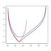
Refer to caption
Figure 8: CD distance in Example 8 when θ^212130subscript^𝜃subscript21subscript21subscript30\hat{\theta}_{2_{1}2_{1}3_{0}} (on the x-axis) is varied: proportional (black), uniform (blue) and order-preserving (red).
Example 9.

Consider two random variables Y1subscript𝑌1Y_{1} and Y2subscript𝑌2Y_{2} and suppose 𝕐1=𝕐2=[3]subscript𝕐1subscript𝕐2delimited-[]3\mathbb{Y}_{1}=\mathbb{Y}_{2}=[3]. Suppose also

θ1i=Pr(Y1=i)=Pr(Y2=i|Y1=j),i[3],j[2].formulae-sequencesubscript𝜃1𝑖Prsubscript𝑌1𝑖Prsubscript𝑌2conditional𝑖subscript𝑌1𝑗formulae-sequence𝑖delimited-[]3𝑗delimited-[]2\theta_{1i}=\Pr(Y_{1}=i)=\Pr(Y_{2}=i\,|\,Y_{1}=j),\,\,\,\,\,i\in[3],j\in[2].

Suppose we let θ11subscript𝜃11\theta_{11} vary and θ12subscript𝜃12\theta_{12} and θ13subscript𝜃13\theta_{13} covary according to a valid scheme. The set ΦΦ\Phi of Proposition 7 is then equal {θ112,θ11θ12,θ13,θ122,θ11θ13,θ12θ13}superscriptsubscript𝜃112subscript𝜃11subscript𝜃12subscript𝜃13superscriptsubscript𝜃122subscript𝜃11subscript𝜃13subscript𝜃12subscript𝜃13\{\theta_{11}^{2},\theta_{11}\theta_{12},\theta_{13},\theta_{12}^{2},\theta_{11}\theta_{13},\theta_{12}\theta_{13}\}. Suppose θ11=0.33subscript𝜃110.33\theta_{11}=0.33, θ12=0.33subscript𝜃120.33\theta_{12}=0.33, θ13=0.34subscript𝜃130.34\theta_{13}=0.34 and let θ11subscript𝜃11\theta_{11} be varied to 0.40.40.4. In this situation the CD distance under a proportional scheme is 2.522.522.52, whilst under a uniform scheme the distance equals 2.502.502.50. For this parameter variation, the uniform scheme would then be preferred to a proportional one if a user wishes to minimize the CD distance. Conversely, if θ11subscript𝜃11\theta_{11} is set to 0.20.20.2 the distance is smaller under the proportional scheme (2.89)2.89(2.89) than under the uniform one (2.92)2.92(2.92).

Therefore, whilst for multilinear models the choice of updating probabilities with a proportional covariation scheme can be justified in terms of some ‘optimality criterion’ based on the minimization of the CD distance, for non-multilinear models the choice of the covariation scheme becomes critical. Our examples demonstrated that inference can be greatly affected by the chosen covariation scheme. With no theoretical justification to use one over another, any output from such a sensitivity analysis of a non-multilinear model will be ambiguous unless a convincing rationale for the choice of the covariation scheme can be found.

We next deduce a closed form expression for the CD distance under the proportional covariation scheme.

Proposition 8.

Under the condition of Proposition 7 and assuming a proportional covariation scheme the CD distance is

CD(𝒑θ,𝒑θ~)=logmax𝜶𝔸C(1θ~i1θi)|𝜶i|θi~αiθiαilogmin𝜶𝔸C(1θ~i1θi)|𝜶i|θi~αiθiαi,\textnormal{CD}(\bm{p}_{\theta},\bm{p}_{\tilde{\theta}})=\log\max_{\bm{\alpha}\in\mathbb{A}_{-C}}\left(\frac{1-\tilde{\theta}_{i}}{1-\theta_{i}}\right)^{|\bm{\alpha}_{-i}|}\frac{\tilde{\theta_{i}}^{\alpha_{i}}}{{\theta_{i}}^{\alpha_{i}}}-\log\min_{\bm{\alpha}\in\mathbb{A}_{-C}}\left(\frac{1-\tilde{\theta}_{i}}{1-\theta_{i}}\right)^{|\bm{\alpha}_{-i}|}\frac{\tilde{\theta_{i}}^{\alpha_{i}}}{{\theta_{i}}^{\alpha_{i}}}, (19)

where 𝔸C0rsubscript𝔸𝐶subscriptsuperscript𝑟0\mathbb{A}_{-C}\in\mathbb{N}^{r}_{0} is the set including the exponents in 𝔸Csubscript𝔸𝐶\mathbb{A}_{C} where the entries relative to indeterminates not in ΘCsubscriptΘ𝐶\Theta_{C} are deleted, 𝛂i0r1subscript𝛂𝑖subscriptsuperscript𝑟10\bm{\alpha}_{-i}\in\mathbb{N}^{r-1}_{0} is an exponent where the entry relative to θisubscript𝜃𝑖\theta_{i} is deleted and |𝛂i|subscript𝛂𝑖|\bm{\alpha}_{-i}| is the sum of its entries.

Proof.

From Proposition 7 we can write the CD distance as

CD(𝒑θ,𝒑θ~)=logmax𝜶𝔸Cϕ~𝜶ϕ𝜶logmin𝜶𝔸Cϕ~𝜶ϕ𝜶.CDsubscript𝒑𝜃subscript𝒑~𝜃subscript𝜶subscript𝔸𝐶superscript~bold-italic-ϕ𝜶superscriptbold-italic-ϕ𝜶subscript𝜶subscript𝔸𝐶superscript~bold-italic-ϕ𝜶superscriptbold-italic-ϕ𝜶\textnormal{CD}(\bm{p}_{\theta},\bm{p}_{\tilde{\theta}})=\log\max_{\bm{\alpha}\in\mathbb{A}_{-C}}\frac{\tilde{\bm{\phi}}^{\bm{\alpha}}}{\bm{\phi}^{\bm{\alpha}}}-\log\min_{\bm{\alpha}\in\mathbb{A}_{-C}}\frac{\tilde{\bm{\phi}}^{\bm{\alpha}}}{\bm{\phi}^{\bm{\alpha}}}.

Recall that under a proportional scheme an indeterminate θjΘC{θi}subscript𝜃𝑗subscriptΘ𝐶subscript𝜃𝑖\theta_{j}\in\Theta_{C}\setminus\{\theta_{i}\} is varied to θ~j=θj(1θ~i)/(1θi)subscript~𝜃𝑗subscript𝜃𝑗1subscript~𝜃𝑖1subscript𝜃𝑖\tilde{\theta}_{j}=\theta_{j}(1-\tilde{\theta}_{i})/(1-\theta_{i}). We then have that, for any ϕΦitalic-ϕΦ\phi\in\Phi,

ϕ~𝜶=θ~iαij[r]{i}(1θ~i1θiθj)αj=(1θ~i1θi)|𝜶i|𝜽i𝜶iθ~iαi,superscript~bold-italic-ϕ𝜶superscriptsubscript~𝜃𝑖subscript𝛼𝑖subscriptproduct𝑗delimited-[]𝑟𝑖superscript1subscript~𝜃𝑖1subscript𝜃𝑖subscript𝜃𝑗subscript𝛼𝑗superscript1subscript~𝜃𝑖1subscript𝜃𝑖subscript𝜶𝑖superscriptsubscript𝜽𝑖subscript𝜶𝑖superscriptsubscript~𝜃𝑖subscript𝛼𝑖\tilde{\bm{\phi}}^{\bm{\alpha}}=\tilde{\theta}_{i}^{\alpha_{i}}\prod_{j\in[r]\setminus\{i\}}\left(\frac{1-\tilde{\theta}_{i}}{1-\theta_{i}}\theta_{j}\right)^{\alpha_{j}}=\left(\frac{1-\tilde{\theta}_{i}}{1-\theta_{i}}\right)^{|\bm{\alpha}_{-i}|}\bm{\theta}_{-i}^{\bm{\alpha}_{-i}}\tilde{\theta}_{i}^{\alpha_{i}},

and therefore

ϕ~𝜶ϕ𝜶=θ~iαiθiαi(1θ~i1θi)|𝜶i|.superscript~bold-italic-ϕ𝜶superscriptbold-italic-ϕ𝜶superscriptsubscript~𝜃𝑖subscript𝛼𝑖superscriptsubscript𝜃𝑖subscript𝛼𝑖superscript1subscript~𝜃𝑖1subscript𝜃𝑖subscript𝜶𝑖\frac{\tilde{\bm{\phi}}^{\bm{\alpha}}}{\bm{\phi}^{\bm{\alpha}}}=\frac{\tilde{\theta}_{i}^{\alpha_{i}}}{\theta_{i}^{\alpha_{i}}}\left(\frac{1-\tilde{\theta}_{i}}{1-\theta_{i}}\right)^{|\bm{\alpha}_{-i}|}.

Then, since CD(𝒑θ,𝒑θ~)=CD(𝒑ϕ,𝒑ϕ~)CDsubscript𝒑𝜃subscript𝒑~𝜃CDsubscript𝒑italic-ϕsubscript𝒑~italic-ϕ\textnormal{CD}(\bm{p}_{\theta},\bm{p}_{\tilde{\theta}})=\textnormal{CD}(\bm{p}_{\phi},\bm{p}_{\tilde{\phi}}) by Proposition 7, we deduce the closed form in equation (19) by substituting the above expression into the definition of CD distance. ∎

Example 10.

Consider again the monomial set ΦΦ\Phi of Example 8 and assume the parameters θ^202130subscript^𝜃subscript20subscript21subscript30\hat{\theta}_{2_{0}2_{1}3_{0}} and θ^222130subscript^𝜃subscript22subscript21subscript30\hat{\theta}_{2_{2}2_{1}3_{0}} are covaried according to a proportional scheme. Call θ^=θ^212130^𝜃subscript^𝜃subscript21subscript21subscript30\hat{\theta}=\hat{\theta}_{2_{1}2_{1}3_{0}} and let x𝑥x be its varied version. From Proposition 8 we can deduce that the CD distance will then depend on the maximum and minimum value in the set of ratios

{x3θ^3,x2θ^2,xθ^,x2θ^2(1x1θ^),xθ^(1x1θ^),(1x1θ^)2,1x1θ^}.superscript𝑥3superscript^𝜃3superscript𝑥2superscript^𝜃2𝑥^𝜃superscript𝑥2superscript^𝜃21𝑥1^𝜃𝑥^𝜃1𝑥1^𝜃superscript1𝑥1^𝜃21𝑥1^𝜃\left\{\frac{x^{3}}{\hat{\theta}^{3}},\frac{x^{2}}{\hat{\theta}^{2}},\frac{x}{\hat{\theta}},\frac{x^{2}}{\hat{\theta}^{2}}\left(\frac{1-x}{1-\hat{\theta}}\right),\frac{x}{\hat{\theta}}\left(\frac{1-x}{1-\hat{\theta}}\right),\left(\frac{1-x}{1-\hat{\theta}}\right)^{2},\frac{1-x}{1-\hat{\theta}}\right\}.

6 Discussion

The definition of a parametric model by its interpolating polynomial has proven useful to investigate how changes in the input probabilities affect an output of interest. We have been able to demonstrate not only that standard results for one-way analyses in BN models are valid for a large number of other models and single full CPT investigations, but also new theoretical justifications for the use of proportional covariation based on a variety of divergence measures. Then, the flexibility of the interpolating polynomial representation enabled us to investigate an even larger class of models, for instance DBNs, extending sensitivity methods to dynamic settings. In this framework both sensitivity functions and CD distances exhibit different properties than in the simpler multilinear case, with the potential of even more informative sensitivity investigations. Importantly, we have been able to produce a new fast procedure to compute the CD distance in non-multilinear models.

Having demonstrated the usefulness of our polynomial approach in single full CPT analyses, we next plan to address the rather more complicated situation of generic multi-way analyses. In particular by representing probabilities in terms of monomials we can relate multi-way analyses in multilinear models to one-way sensitivities in non-multilinear ones. It can be seen that sensitivity functions for multi-way analyses will not simply be multilinear but also include interaction terms. Similarly, the CD distance will be affected by such interactions and not simply correspond to the CD distance of the appropriate CPT. Example 9 would therefore suggest that the proportional covariation scheme is not optimal in this context. However, we notice that the monomials from multi-way analyses in multilinear models are a subset of those arising from non-multilinear ones. Although these can be of an arbitrary degree, each indeterminate of the monomial will have exponent one by construction. Therefore, there is no conclusive proof of the non-optimality of the proportional scheme in generic multi-way analyses for multilinear models and BNs. However the polynomial representation of probabilities in BNs and related models gives us a promising starting point to start investigating this class of problems.

Acknowledgements

M. Leonelli was supported by Capes, C. Görgen was supported by the EPSRC grant EP/L505110/1 and J. Q. Smith was supported by the EPSRC grant EP/K039628/1.

References

References

  • Aguilera et al. [2011] P. A. Aguilera, A. Fernández, R. Fernández, R. Rumí, and A. Salmerón. Bayesian networks in environmental modelling. Environ. Modell. Softw., 26:1376–1388, 2011.
  • Ali and Silvey [1966] S. M. Ali and S. D. Silvey. A general class of coefficients of divergence of one distribution from another. J. Roy. Statist. Soc. Ser. B, 28:131–142, 1966.
  • Anacleto and Queen [2013] O. Anacleto and C. M. Queen. Dynamic chain graph models for multivariate time series. Technical report, Department of Statistics, Open University, 2013.
  • Barclay et al. [2015] L. M. Barclay, R. A. Collazo, J. Q. Smith, P. A. Thwaites, and A. E. Nicholson. The dynamic chain event graph. Electron. J. Stat., 9:2130–2169, 2015.
  • Bolt and van der Gaag [2015] J. H. Bolt and L. C. van der Gaag. Balanced tuning of multi-dimensional Bayesian network classifiers. In Symbolic and Quantitative Approaches to Reasoning with Uncertainty, pages 210–220. Springer, 2015.
  • Boutilier et al. [1996] C. Boutilier, N. Friedman, M Goldszmidt, and D. Koller. Context-specific independence in Bayesian networks. In Proceedings of the 12th Conference on Uncertainty in Artiificial Intelligence, pages 115–123, 1996.
  • Cano et al. [2004] R. Cano, C. Sordo, and J. M. Gutiérrez. Applications of Bayesian networks in meteorology. In Advances in Bayesian Networks, pages 309–328. Springer, 2004.
  • Castillo et al. [1997] E. Castillo, J. M. Gutiérrez, and A. S. Hadi. Sensitivity analysis in discrete Bayesian networks. IEEE T. Syst. Man Cyb., 27:412–423, 1997.
  • Chan and Darwiche [2002] H. Chan and A. Darwiche. When do numbers really matter? J. Artificial Intelligence Res., 17:265–287, 2002.
  • Chan and Darwiche [2004] H. Chan and A. Darwiche. Sensitivity analysis in Bayesian networks: from single to multiple parameters. In Proocedings of the 16th Conference on Uncertainty in Artificial Intelligence, pages 317–325, 2004.
  • Chan and Darwiche [2005a] H. Chan and A. Darwiche. A distance measure for bounding probabilistic belief change. Internat. J. Approx. Reason., 38:149–174, 2005a.
  • Chan and Darwiche [2005b] H. Chan and A. Darwiche. Sensitivity analysis in Markov networks. In Proocedings of the 19th International Joint Conference on Artificial Intelligence, pages 1300–1305, 2005b.
  • Charitos and van der Gaag [2006a] T. Charitos and L. C. van der Gaag. Sensitivity analysis of Markovian models. In Proceedings of the FLAIRS Conference, pages 806–811, 2006a.
  • Charitos and van der Gaag [2006b] T. Charitos and L. C. van der Gaag. Sensitivity analysis for threshold decision making with dynamic networks. In Proceedings of the 22nd Conference on Uncertainty in Artificial Intelligence, pages 72–79, 2006b.
  • Chen and Pollino [2012] S. H. Chen and C. A. Pollino. Good practice in Bayesian network modelling. Environ. Modell. Softw., 37:134–145, 2012.
  • Coupé and van der Gaag [2002] V. M. H. Coupé and L. C. van der Gaag. Properties of sensitivity analysis of Bayesian belief networks. Ann. Math. Artif. Intell., 36:323–356, 2002.
  • Cowell et al. [1999] R. G. Cowell, A. P. Dawid, Lauritzen S. L., and D. J. Spiegelhalter. Probabilistic networks and expert systems. Springer-Verlag, New York, 1999.
  • Csiszár [1963] I. Csiszár. Eine informationstheoretische ungleichung und ihre anwendung auf den beweis der ergodizität von markoffschen ketten. Magyar Tud. Akad. Mat. Kutató Int. Közl., 8:85–108, 1963.
  • Dagum and Horvitz [1993] P. Dagum and E. Horvitz. A Bayesian analysis of simulation algorithms for inference in belief networks. Networks, 23:499–516, 1993.
  • Darwiche [2003] A. Darwiche. A differential approach to inference in Bayesian networks. J. ACM, 3:280–305, 2003.
  • Drton et al. [2009] M. Drton, B. Sturmfels, and S. Sullivant. Lectures on algebraic statistics. Birkhäuser Verlag, Basel, 2009.
  • French [2003] S. French. Modelling, making inferences and making decisions: the roles of sensitivity analysis. Top, 11:229–251, 2003.
  • Gómez-Villegas et al. [2007] M. A. Gómez-Villegas, P. Main, and R. Susi. Sensitivity analysis in Gaussian Bayesian networks using a divergence measure. Comm. Statist. Theory Methods, 36:523–539, 2007.
  • Gómez-Villegas et al. [2013] M. A. Gómez-Villegas, P. Main, and R. Susi. The effect of block parameter perturbations in Gaussian Bayesian networks: sensitivity and robustness. Inform. Sci., 222:429–458, 2013.
  • Görgen and Smith [2015] C. Görgen and J. Q. Smith. Equivalence classes of staged trees. Technical report, CRISM 15-12, University of Warwick, 2015.
  • Görgen et al. [2015] C. Görgen, M. Leonelli, and J. Q. Smith. A differential approach for staged trees. In Symbolic and Quantitative Approaches to Reasoning with Uncertainty, pages 346–355. Springer, 2015.
  • Heckerman et al. [1995] D. Heckerman, A. Mamdani, and M. P. Wellman. Real-world applications of Bayesian networks. Commun. ACM, 38:24–26, 1995.
  • Jeffreys [1946] H. Jeffreys. An invariant form for the prior probability in estimation problems. Proc. Roy. Soc. London Ser. A, 186:453–461, 1946.
  • Jordan [2004] M. I. Jordan. Graphical models. Statist. Sci., 19:140–155, 2004.
  • Koller and Lerner [2001] D. Koller and U. Lerner. Sampling in factored dynamic systems. In Sequential Monte Carlo Methods in Practice, pages 445–464. Springer, 2001.
  • Korb and Nicholson [2010] K. Korb and A. E. Nicholson. Bayesian artificial intelligence. CRC Press, Boca Raton, 2010.
  • Kullback and Leibler [1951] S. Kullback and R. A. Leibler. On information and sufficiency. Ann. Math. Statistics, 22:79–86, 1951.
  • Lauritzen [1996] S. L. Lauritzen. Graphical models. Oxford University Press, Oxford, 1996.
  • Low-Choy et al. [2012] S. Low-Choy, A. James, J. Murray, and K. Mengersen. Elicitator: a user-friendly interactive toll to support scenario-based elicitation of expert knowledge. In Expert Knowledge and its Application in Landscape Ecology, pages 39–67. Springer, 2012.
  • Murphy [2002] K. P. Murphy. Dynamic Bayesian networks: representation, inference and learning. PhD thesis, University of California, Berkeley, 2002.
  • Neil et al. [2000] M. Neil, N. Fenton, and L. Nielson. Building large-scale Bayesian networks. Knowl. Eng. Rev., 15:257–284, 2000.
  • Pardo [2005] L. Pardo. Statistical inference based on divergence measures. CRC Press, Boca Raton, 2005.
  • Pearl [1988] J. Pearl. Probabilistic reasoning in intelligent systems. Morgan-Kauffman, San Francisco, 1988.
  • Pensar et al. [2016] J. Pensar, H. Nyman, J. Lintusaari, and J. Corander. The role of local partial independence in learning of Bayesian networks. Intern. J. Approx. Reason., 69:91–105, 2016.
  • Pistone et al. [2001] G. Pistone, E. Riccomagno, and H. P. Wyn. Gröbner bases and factorisation in discrete probability and Bayes. Stat. Comput., 11:37–46, 2001.
  • Pitchforth and Mengersen [2013] J. Pitchforth and K. Mengersen. A proposed validation framework for expert elicited Bayesian networks. Expert Syst. Appl., 40:162–167, 2013.
  • Pollino et al. [2007] C. A. Pollino, O. Woodberry, A. Nicholson, K. Korb, and B. T. Hart. Parameterisation and evaluation of a Bayesian network for use in an ecological risk assessment. Environ. Modell. Softw., 22:1140–1152, 2007.
  • Rajabally et al. [2004] E. Rajabally, P. Sen, S. Whittle, and J. Dalton. Aids to Bayesian belief network construction. In Proceedings of the 2nd International Conference on Intelligence Systems, pages 457–461, 2004.
  • Renooij [2012] S. Renooij. Efficient sensitivity analysis in hidden Markov models. Internat. J. Approx. Reason., 53:1397–1414, 2012.
  • Renooij [2014] S. Renooij. Co-variation for sensitivity analysis in bayesian networks: properties, consequences and alternatives. Internat. J. Approx. Reason., 55:1022–1042, 2014.
  • Riccomagno [2009] E. Riccomagno. A short history of algebraic statistics. Metrika, 69:397–418, 2009.
  • Smith and Anderson [2008] J. Q. Smith and P. E. Anderson. Conditional independence and chain event graphs. Artificial Intelligence, 172:42–68, 2008.
  • van der Gaag et al. [2007] L. C. van der Gaag, S. Renooij, and V. M. H. Coupé. Sensitivity analysis of probabilistic networks. In Advances in Probabilistic Graphical Models, pages 103–124. Springer, 2007.