Present Address: ]Department of Physics, University of Cyprus, P.O. Box 20537, 1678 Nicosia, Cyprus and Department of Physics, Bergische Universität Wuppertal Gaussstr. 20, 42119 Wuppertal, Germany.
dependence in Yang-Mills theory from analytic continuation
Abstract
We investigate the topological properties of the pure gauge theory by performing numerical simulations at imaginary values of the parameter. By monitoring the dependence of various cumulants of the topological charge distribution on the imaginary part of and exploiting analytic continuation, we determine the free energy density up to the sixth order in , . That permits us to achieve determinations with improved accuracy, in particular for the higher order terms, with control over the continuum and the infinite volume extrapolations. We obtain and .
pacs:
12.38.Aw, 11.15.Ha, 12.38.GcI Introduction
The non-trivial consequences related to the possible presence of a topological parameter are among the most interesting properties of non-abelian gauge theories. That enters the Euclidean Yang-Mills Lagrangian as follows
| (1) |
where
| (2) |
is the topological charge density; is a superselected parameter, characterizing the vacuum as well as the other physical states of the theory. The topological charge density is odd under symmetry, hence a non-zero value would break such symmetry explicitly.
Experimental upper bounds on are quite stringent (), nevertheless, the dependence of Quantum ChromoDynamics (QCD) and of gauge theories on enters various aspects of hadron phenomenology, a paradigmatic example being the solution of the problem 'tHooft:1976up ; Witten:1979vv ; Veneziano:1979ec . By CP symmetry at , the free energy density of the theory is an even function of which can be parametrized as follows
| (3) |
where is the topological susceptibility, while is a dimensionless even function of , normalized as , which, assuming analyticity around , can be expanded as follows
| (4) |
The dependence on , being related to the topological properties of the theory, is of inherent non-perturbative nature. Therefore analytic predictions are restricted to particular regimes or effective approximation schemes Gross:1980br ; schschrev ; Zhitnitsky:2008ha ; Unsal:2012zj ; Poppitz:2012nz ; Anber:2013sga ; Bigazzi:2015bna . For instance, at asymptotically high temperatures the Dilute Instanton Gas Approximation is expected to hold, which predicts , while regarding the low-temperature phase and the -dependence of the ground state energy, large- arguments Witten-98 ; Witten-80 predict the various non-linear terms in to be suppressed by increasing powers of , in particular (see e.g. Vicari:2008jw for a general review of the subject).
Lattice QCD represents a valid non-perturbative approach, which is based on first principles only, however the complex nature of the Euclidean action in Eq. (1) hinders direct Monte-Carlo simulations at non-zero . Some possible, partial solutions to this problem are similar to the ones adopted for QCD at finite baryon chemical potential , where the fermion determinant becomes complex. In particular, assuming analyticity around , one can either obtain the free energy density in terms of its Taylor expansion coefficients computed at (see Refs. taylormu1 ; taylormu2 ; taylormu3 for analogous strategies at ), or perform numerical simulations at imaginary values of azcoiti ; alles_1 ; alles_2 ; aoki_1 ; pavim ; dene (or immu1 ; immu2 ; immu3 ; immu4 ; mdfs1 ; tadena ) and then exploit analytic continuation.
The first strategy has been traditionally adopted for the study of dependence. The topological susceptibility and the coefficients are proportional to the coefficients of the Taylor expansion in and can be directly computed in terms of the cumulants of the probability distribution at of the global topological charge . For instance the first few terms are given by
| (5) |
where is the four-dimensional volume,
| (6) |
and
| (7) |
As we will discuss in more detail in the following, a drawback of this approach is that the coefficients of the non-quadratic terms, , are determined as corrections to a purely gaussian behavior for the probability distribution of the topological charge at . By the central limit theorem, such corrections are less and less visible as the total four-dimensional volume increases, so that a significant increase in statistics is needed, in order to keep a constant statistical error, as one tries to increase in order to keep finite size effects under control.
This problem can be avoided with the approach based on analytic continuation from an imaginary . In this case, one typically determines a derivative of the free energy as a function of : for instance one has
| (8) |
and is obtained as a deviation from linearity of the response of the system to the external source , which is determined with no loss in accuracy as the system size is increased. A drawback in this case is represented by a finite renormalization appearing when the external source is added to the discretized theory; nevertheless, the method of analytic continuation turns out to be the most suitable to a high precision study of the coefficients , which must keep both finite size and discretization errors under control.
In this study we investigate the -dependence of pure gauge theory using the analytic continuation approach. We will explore variants of the original strategy presented in Ref. pavim , in particular we will perform a simultaneous fit to various derivatives of the free energy density as a function of , in analogy with a similar approach explored in lattice QCD at imaginary chemical potential tadena . That will permit us to maximize the information obtained from our numerical simulations and, at the same time, to determine the finite renormalization constant as a parameter of the global fit. That will result in an increased precision, which will give us the opportunity to determine a continuum extrapolated value of with an uncertainty at the level of a few percent.
II Numerical method
The free energy density of Yang-Mills theory in the presence of a term is given by
| (9) |
where is the standard euclidean action of Yang-Mills theory, is the topological charge and periodic boundary conditions are assumed. As discussed in the introduction it is not possible to use directly this form in a Monte Carlo simulation, since the action is not real for . To overcome this problem we will study the theory for imaginary values of , where standard importance sampling methods can be applied, using the analytic continuation of Eqs.(3), (4) to extract the values of the coefficients.
In practice, one defines , where is a real parameter, and studies the dependence of
| (10) | ||||
From Eq. (9) it follows that the derivatives of can be written as
| (11) |
where are the cumulants of the topological charge distribution at fixed . Since for the CP symmetry is explicitly broken, also the odd cumulants are generically non-vanishing. Using Eq. (11) together with the expansion in Eq. (10) we obtain an infinite chain of equations relating the cumulants of the topological charge to the coefficients and . The first few of these equations are the following
| (12) |
The general idea of the analytic continuation method is to perform Monte Carlo simulations at several values of , to compute some of the cumulants for each and to extract the coefficients , making use Eq. (12).
It is clear that in this procedure one can adopt different strategies. Each of the relations in Eq. (12) is itself sufficient to extract all the parameters, at least from a given order on: for example can be estimated by looking at the leading linear dependence of on or by looking at the small value of . While all these methods are equally valid from the theoretical point of view, they are not equivalent in computational efficiency, since at fixed statistics lower cumulants are determined with better accuracy (see Sec. III.1 for a detailed discussion on this point). On the other hand the computation of higher cumulants does not require new simulations or even new measurements, so that if we use also higher momenta we increase the information available at no additional cost. What appears to be the optimal strategy is to extract and from a combined fit of all the relations in Eq. (12). Since higher momenta get more and more noisy, it is natural to expect that, at some point, adding to the global fit still higher cumulants will not result in an increased precision, however it is not a priori clear when this will happen; in the following analysis we will use up to the fourth cumulant. Obviously, in order to correctly assess the statistical uncertainties of the extracted parameters, correlations among the cumulants have to be taken into account.
II.1 Lattice implementation and topological charge definition
Various methods exist to determine the topological content of lattice configurations, either based on fermionic or gluonic definitions, which have proven to provide consistent results as the continuum limit is approached (see Ref. Vicari:2008jw for a review). Gluonic definitions are typically affected by renormalizations related to fluctuations at the ultraviolet (UV) cutoff scale, which can be cured by a proper smoothing of gauge configurations. Cooling cooling1 ; cooling2 ; cooling3 ; cooling4 ; cooling5 is a standard procedure adopted to do that; recently the gradient flow Luscher:2009eq ; Luscher:2010iy has been introduced, which has been shown to provide results equivalent to cooling, at least regarding topology Bonati:2014tqa ; Cichy:2014qta ; Namekawa:2015wua ; Alexandrou:2015yba .
However, for the purpose of inserting a -term in the action, the use of a fermionic or of a smoothed gluonic definition of is impractical. The lattice partition function in the presence of an imaginary -term reads
| (13) |
where stands for the gauge link variables, , is the lattice pure gauge action and is the discretized topological charge. Standard efficient algorithms like heat-bath, which are available for pure gauge theories, are applicable in this case only if a particularly simple discretization of the topological charge density is chosen, while other choices would lead to a significant computational overhead. In our case, we choose the standard Wilson plaquette action for and the simplest discretization of with definite parity DiVecchia:1981qi ; DiVecchia:1981hh :
| (14) |
where is the plaquette operator, for positive directions, while and antisymmetry fix its value in the generic case. With this choice, gauge links still appear linearly in the Boltzmann weight, so that standard heat-bath and over-relaxation algorithms can be implemented, with a computational cost that is about a factor 2.5 higher than at .
A drawback of this choice is that takes a finite multiplicative renormalization with respect to the continuum density Teper:1989ig ; Campostrini:1989dh ; DiGiacomo:1989id ; DiGiacomo:1991ba
| (15) |
where is the lattice spacing and . Hence, the lattice parameter is related to the imaginary part of by : in order to know , one has to determine the value .
As for the operator used to determine the cumulants of the topological charge distribution, in order to avoid the appearance of further renormalization constants, we adopt a smoothed definition which is denoted simply as in the following. In particular, we adopt the topological charge density in Eq. (14), measured after cooling steps. Actually, in this case two possible prescriptions can be taken. One can simply define : in this case, at finite lattice spacing, does not take exactly integer values, although its distribution is characterized by sharp peaks located at approximately integer values. In alternative, one can define as follows DelDebbio:2002xa :
| (16) |
where denotes the integer closest to and the rescaling factor is determined in such a way to minimize
| (17) |
so that the sharp peaks in the distribution of will be located exactly onto integer values. The two definitions are expected to coincide as the continuum limit is approached. In the following we will refer to the latter as the rounded topological charge and to the former as the non-rounded one. The two definitions have been used alternately in various previous studies in the literature. In this study we consider both of them and show that, while results at finite lattice spacing differ, continuum extrapolated results coincide, as expected.
In order to make use of Eqs. (12) to obtain the free energy parameters from the -dependence of the cumulants of , one needs to know the values of used for each numerical simulation. That in turn requires a determination of the renormalization constant . Various methods exist to do that, for instance by using the relation pavim
| (18) |
or other similar approaches, like heating techniques DiGiacomo:1991ba . However, a drawback of this approach is that the statistical uncertainty on propagates to , so that a non-trivial fit with errors on both dependent and independent variables is required. For that reason in this study we investigate and adopt a different approach.
We rewrite a lattice version of Eqs. (12) in which the lattice parameter appears explicitly:
| (19) |
Our proposal is to extract the renormalization constant from the fitting procedure itself, treating as the independent variable and as a fit parameter. Notice however that, in order to do that, at least two cumulants must be fitted simultaneously, otherwise remains entangled as an arbitrary multiplicative renormalization of the other fit parameters. On the other hand, fitting the dependence of more cumulants at the same time coincides with our proposed strategy to extract the best possible information from our Monte-Carlo simulations. As we will show in the next section, the payoff of this strategy is not negligible.
III Numerical results
| [fm] | ||
|---|---|---|
| 5.95 | 4.898(12) | 0.1021(25) |
| 6.07 | 6.033(17) | 0.08288(23) |
| 6.20 | 7.380(26) | 0.06775(24) |
| 6.40 | 9.74(5) | 0.05133(26) |
| 5.95 | 0,2,4,6,8 | |
| 6.07 | 0,2,4,6,8,10 | |
| 6.20 | , , , | 0,2,4,6,8,10,12 |
| 6.40 | 0,2,4,6,8,10,12,14 | |
| 6.173 | 0,2,4,6,8,10,12 |
We have performed simulations at four different lattice spacings on hypercubical lattices; the values of the bare parameters adopted are reported in Tabs. 1-2. The Monte Carlo updates were performed using a mixture of standard heatbath Creutz1980 ; KP and overrelaxation Creutz1987 algorithms, implemented à la Cabibbo-Marinari CM , in the ratio of 1 to 5. The topological charge was measured every updates and from 5 to 25 cooling steps were used: data that will be presented in the following refer to the case of 15 cooling steps and we checked that results are stable, well within errors, if a different choice is made.
Unless otherwise explicitly stated, we present data which refer to the case of a common fit to the first four cumulants of the topological charge, see Eq. (19). An example of such a fit is reported in Fig. 1. Since cumulants of different order are computed on the same samples of gauge configurations, in order to take into account the possible correlations among them we have used a bootstrap procedure, and checked that a correlated fit exploiting the full covariance matrix leads to consistent results.
In the following we
are going to illustrate our estimation of the various possible
systematic uncertainties that may affect our results. First, we will analyze
those related to analytic continuation itself, by considering the stability
of our fits as either the fit range or the number of fitted terms
in Eq. (19) (i.e. the truncation of the Taylor series)
is changed; then we will turn to the analysis of the infinite volume
and continuum limit extrapolations.
That will permit us to provide final estimates of the free energy
coefficients entering Eqs. (3) and (4), with
a reliable determination of both statistical and systematic uncertainties.
In the last part of our analysis we will try to understand which aspects
of our strategy lead to a more significant improvement with respect
to other methods used in the past literature.
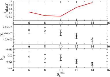
In Fig. 2 we report an example of how the fitted coefficients and the quality of the fit change as a function of the range of imaginary values of included in the fit, in particular of the maximum value . The final range from which we extract our determination is chosen so as to have a reasonable value of the test and stability, within errors, of the fitted parameters as the range is reduced further: this is important to ensure the reliability of analytic continuation, since the expressions in Eq. (19) are expected to hold, in principle, in a limited range around . A full account of the ranges used in the various cases is reported in Tab. 2.
We notice that grows as one approaches the continuum limit. That can be interpreted by observing that, since growing values of induce growing values of the net non-zero topological charge density, one may expect saturation effects to be present for large enough values of . Such effects are expected to appear earlier on lattices with less resolution, i.e. with larger values of the lattice spacing.
A source of systematic error that is generically present in the analytic continuation approach is the one related to the choice of the fitting function, in particular to the truncation of the series to be fitted. In the present work, the estimated value of turns out to be compatible with zero for all the data sets, so it appears reasonable to fix the value of to zero and fit just , and . To check that this does not introduce any significant systematic error we verified that fits with fixed well describe data and give results compatible with the ones obtained by fitting also .
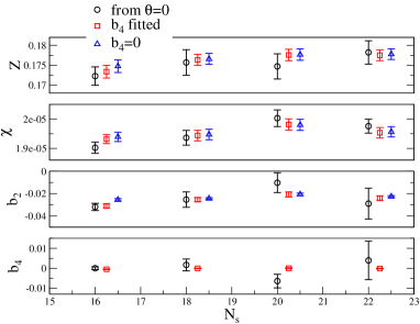
In order to investigate finite size effects, we have explored different lattice sizes for one case, in particular corresponding to a lattice spacing fm. In Fig. 3 we report the corresponding results obtained both from analytic continuation and from a direct measurement of the cumulants at . We notice that errors on and obtained from analytic continuation scale much better as the volume is increased (the underlying reason is discussed in Sec. III.1), so that in this case one can investigate finite size effects with much more reliability than with a traditional approach based on simulations only. One could try to estimate the infinite volume limit by explicitly fitting the volume dependence of the results, which is expected to decay exponentially with , however it is clearly visible from the figure that finite size effects are negligible within errors for lattices with , i.e. for fm. Lattices explored at the other values of the lattice spacing have been chosen accordingly, i.e. they correspond to linear sizes which are well above this threshold ( at least).
| # measures | |||
| 5.96 | 240K, 130K | 3.47(8) | |
| 6.07 | 110K, 70K | 4.8(2) | |
| 6.20 | 170K, 60K | 18(1) | |
| 6.20 | 100K, 70K | 17(1) | |
| 6.20 | 100K, 90K | 17(1) | |
| 6.20 | 110K, 80K | 16(1) | |
| 6.40 | 200K, 120K | 214(30) | |
| 6.173 | 50K, 20K | 27(3) |
| rounded | |||
|---|---|---|---|
| 5.95 | |||
| 6.07 | |||
| 6.20 | |||
| 6.40 | |||
| non-rounded | |||
| 5.95 | 0.13838(36) | ||
| 6.07 | 0.16300(73) | ||
| 6.20 | 0.1900(14) | ||
| 6.40 | 0.2185(28) | ||
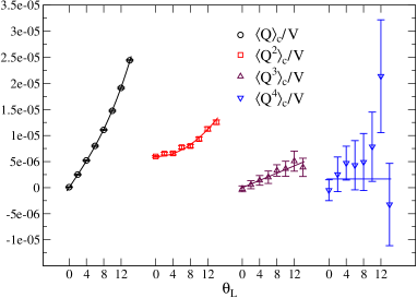
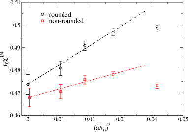
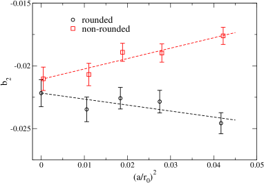
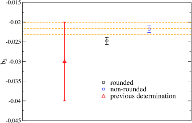
Let us now go to a discussion of the continuum limit. In order to have better control on the systematics of the continuum extrapolation, we used two different definitions of the topological charge, the rounded and the non-rounded one, see Sec. II.1. Since the two definitions are expected to coincide in the continuum limit and they were measured on the same set of gauge configurations, the differences obtained for the continuum extrapolated values in the two cases can be used as an estimate of the residual systematic uncertainties on the final results. In Fig. 4 we report results obtained for the topological susceptibility as a function of , where is the Sommer scale parameter Sommer:1993ce . In both cases (rounded and non-rounded) finite cut-off effects can be reasonably fitted by a quadratic function of if the three finest lattices are considered. Our final estimate is
| (20) |
where the first error is the statistical one and the second the systematic one; this value is compatible with previous determinations Alles:1996nm ; DelDebbio:2002xa ; DelDebbio:2004ns ; Durr:2006ky ; Luscher:2010ik ; Cichy:2015jra ; Ce:2015qha and has a similar error. The conversion to physical units can be performed e.g. using (from Ref. Garden:1999fg ) and the experimental value , thus obtaining . The first error originates from the uncertainty in (the systematic and statistical components were summed in quadrature), while the second error is related to the scale setting and it is the dominant one.
A similar analysis for is reported in Fig. 5. In this case our final result is
| (21) |
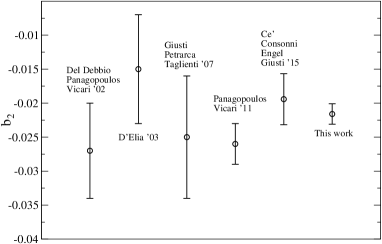
where again the numbers in parentheses are, from left to right, the statistical and the systematic error. This number is compatible with previous results in the literature DelDebbio:2002xa ; D'Elia:2003gr ; Giusti:2007tu ; pavim ; Ce:2015qha , as can be appreciated from Fig. 6 where we report a summary of all existing determinations, however a sizable error reduction has been achieved in the present study.
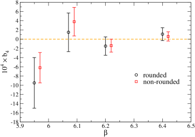
Finally, as we have already emphasized, we do not find any evidence of a nonvanishing coefficient, so the best we can do is to set an upper bound to its absolute value. In Fig. 7 we show the results obtained by using a combined fit for the first four cumulants, with , , and as fit parameters. All data are compatible with zero and a reasonable upper bound appears to be
| (22) |
III.1 Comparison with the efficiency of other approaches
As we have already emphasized, Fig. 3 shows that, at least for the higher order cumulants, the gain in statistical accuracy obtained by analytic continuation with respect to a direct determination at becomes overwhelming as the lattice volume grows. We are now going to understand why.
The cumulants of the topological charge distribution, , are proportional to the coefficients of the Taylor expansion of the free energy as a function of . Since the free energy is an extensive quantity, the cumulants are extensive as well, therefore scales proportionally to the four-dimensional volume , and the ratios of cumulants, i.e. the coefficients entering the free energy density, are volume independent. On the other hand, in the large volume limit the probability distribution of the topological charge is dominated by Gaussian fluctuations with variance , hence the typical fluctuation has size . Since at the distribution of is centered around zero, one has that the terms that sum up to (i.e. ) grow like . Therefore the cumulant itself, which is of order , comes out from the precise cancellation of higher order terms, so that the signal-to-noise ratio is expected to scale like
This is consistent with the fact that the cumulants measure the deviations from a purely Gaussian distribution, and such deviations, because of the central limit theorem, become less and less visible as the infinite volume limit is approached.
We conclude that the error expected in the standard determination of through the cumulants at is of the order of , where is the size of the statistical sample, i.e. the number of independent gauge configurations. This is a particularly severe case of lacking of self-averaging MBH , for instance in the case of one has to increase the number of measurement proportionally to , in order to keep a fixed statistical accuracy as the volume is increased. Notice that this problem is not marginal. Indeed, the important parameter entering this scaling is the combination : since , we expect a strong degradation in the signal-to-noise ratio as one approaches lattices which exceed one fermi in size, which is consistent with our observations; unfortunately, this is also at a threshold where finite size effects are still important.
On the contrary, when using the analytic continuation approach, this problem disappears. Indeed, in this case the information about each free energy coefficient is contained also in the dependence of the lowest order cumulants, including , whose signal to noise ratio scales with volume as . The improvement is related to the fact that one is probing the system with an explicit non-zero external source, and is similar to that obtained when switching from the measurement of fluctuations to the measurement of the magnetization as a function of the external field in the determinations of the magnetic susceptibility of a material.
Therefore, one expects that the final statistical accuracy at fixed number of measurements, improves when increasing the volume, rather than degrading, like for standard self-averaging quantities. Actually, in the particular case of the analytic continuation in , there is a slight complication related to the renormalization constant . This can be computed as in Eq. (18), but in this case we need also , whose precision scales like with volume. The method of global fit is not qualitatively better in this respect: since appears as a rescaling of it cannot be determined just by using the first cumulant, its value is fixed by the comparison of at least and and the precision of the second scales as . We thus see that the best we can obtain with the analytic continuation approach is a scaling of the precision of with volume like ; this is suboptimal with respect to the naive expectation , but still a tremendous improvement with respect to the Taylor expansion method. On the other hand, the precisions of and scale in both approaches as .
All these scalings, and the improvement gained by analytic continuation, can be
nicely seen in Fig. 3. Three determinations of , and
are shown: the first one is obtained by using the Taylor expansion
method, i.e using just the sets, the second one uses the analytic
continuation approach, including in the global fit up to the fourth cumulant of
the topological charge and fitting , , and , the last one
follows the same strategy as the second one but is fixed to zero in the
fit. The determination of obviously used only the first two methods.
Actually, a reasonable comparison between different methods should proceed
along the following lines: compare the errors obtained by different approaches
when using the same machine-time. For the comparison to be fair we thus have to
rescale the statistics of the determination by about a factor of
, i.e. the errors of the corresponding determination by about a factor of
. We thus see that no gain is obtained by using the analytic continuation
approach to determine and , while it is extremely beneficial for
and , as theoretically expected.
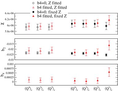
A last point that remains to be investigated is the effectiveness, within the analytic continuation approach, of the global fit to all the cumulants with respect to the traditional procedure of using just , with fixed using Eq. (18). Such a comparison is performed in Fig. 8, in which also intermediate cases are shown: a global fit of all the parameters using different numbers of cumulants or a global fit of all the parameters but (which was fixed by Eq. (18)), using different numbers of cumulants. As can be seen the inclusion in the fit of cumulants of order higher than the second does not improve appreciably the precision of the result; the error reduction attainable by fitting also instead of fixing it before the fit is not huge, but still significant. Indeed, by using all the cumulants of the topological charge and fitting we reduced the errors by about a factor of with respect to the traditional procedure of using just with fixed by Eq. (18).
III.2 Some considerations about the finite temperature case
A strategy allowing to measure on arbitrary large volumes represents a substantial improvement, that permits to gain in statistical accuracy and reduces the possible systematics related to finite size effects. There are however cases in which this possibility is not just an “improvement”, but it enables the study of otherwise intractable problems. This is the case of at finite temperature for . Once the lattice spacing is fixed and the temperature is fixed (i.e. and are fixed), to ensure that we are studying a finite temperature system we have to impose the constraint (typically is used) and this fixes a lower value for the acceptable four-volumes to be used. What typically happens is that this minimum value of is large enough to make a measure of using the Taylor expansion method extremely difficult.
In order to verify that the analytic continuation approach works equally well also at finite temperature, we performed a simulation at on a lattice . Such a point was previously investigated in Bonati:2013tt using the Taylor expansion method. The result from Ref. Bonati:2013tt , together with our new determinations and the result are reported in Fig. 9. The old determination of Ref. Bonati:2013tt was based on a statistics of about measures: our present determination obtained via analytic continuation reaches a precision which is more than one order of magnitude larger, with about half the computational effort (in particular, a machine-time equivalent to around measures taken at ).
Different considerations should be made for temperatures above the critical temperature . Indeed, in all the recent studies of at finite temperature Bonati:2013tt ; Bonati:2015uga ; Borsanyi:2015cka ; Xiong:2015dya (in which the Taylor expansion method was always used) it was noted that the determination of in the low temperature phase is very difficult, while it gets abruptly easier above deconfinement. The reason for this fact is simple: we have seen that the relevant parameter for the degradation of the statistical accuracy in the determination of the cumulants at is . Since at the deconfinement transition the topological susceptibility steeply decreases Alles:1996nm ; Gattringer:2002mr ; Lucini:2004yh ; DelDebbio:2004rw ; Berkowitz:2015aua ; Kitano:2015fla ; Borsanyi:2015cka ; Xiong:2015dya , a precise determination of by the standard Taylor expansion approach becomes much easier, in the deconfined phase, even on moderately large volumes.
IV Conclusions
In this study we have exploited numerical simulations performed at imaginary values of and analytic continuation in order to determine the dependence of the free energy density of the pure gauge theory on the topological parameter . As an improvement with respect to previous applications of the same strategy pavim , we have considered a global fit to the dependence of various free energy derivatives, i.e. various cumulants of the topological charge distribution. That has permitted us to reach an increased precision, obtaining the following estimates for the continuum extrapolated values: , and .
The strategy based on analytic continuation turns out to be particularly well suited for the determination of the higher order terms, for which the traditional Taylor expansion method, based on the determination of cumulants of the topological charge distribution at , faces a severe problem when approaching large volumes, where corrections to Gaussian-like fluctuations become hardly measurable. Indeed, we have shown that the statistical error attained in the determination of through the cumulants at scales with the four-dimensional volume , for a fixed number of measurements, like , where is the topological susceptibility. As we have shown, this property of analytic continuation turns out to be essential for the determination of -dependence right below the deconfinement temperature , hence this strategy could be adopted for a future improved determination of the change of -dependence taking place at deconfinement Bonati:2013tt .
Acknowledgements.
We thank Francesco Negro and Ettore Vicari for useful discussions. Numerical simulations have been performed on the CSN4 cluster of the Scientific Computing Center at INFN-PISA and on the Galileo machine at CINECA (under INFN project NPQCD). Work partially supported by the INFN SUMA Project.References
- (1) G. ’t Hooft, Phys. Rev. Lett. 37, 8 (1976).
- (2) E. Witten, Nucl. Phys. B 156, 269 (1979).
- (3) G. Veneziano, Nucl. Phys. B 159, 213 (1979).
- (4) D. J. Gross, R. D. Pisarski and L. G. Yaffe, Rev. Mod. Phys. 53, 43 (1981).
- (5) T. Schaefer and E. V. Shuryak, Rev. Mod. Phys. 70, 323 (1998) [hep-ph/9610451].
- (6) A. R. Zhitnitsky, Nucl. Phys. A 813, 279 (2008) [arXiv:0808.1447 [hep-ph]].
- (7) M. Unsal, Phys. Rev. D 86, 105012 (2012) [arXiv:1201.6426 [hep-th]].
- (8) E. Poppitz, T. Schaefer and M. Unsal, JHEP 1303, 087 (2013) [arXiv:1212.1238 [hep-th]].
- (9) M. M. Anber, Phys. Rev. D 88, 085003 (2013) [arXiv:1302.2641 [hep-th]].
- (10) F. Bigazzi, A. L. Cotrone and R. Sisca, JHEP 1508, 090 (2015) [arXiv:1506.03826 [hep-th]].
- (11) E. Witten, Phys. Rev. Lett. 81, 2862 (1998).
- (12) E. Witten, Ann. Phys. (NY) 128, 363 (1980).
- (13) E. Vicari and H. Panagopoulos, Phys. Rept. 470, 93 (2009) [arXiv:0803.1593 [hep-th]].
- (14) C. R. Allton, S. Ejiri, S. J. Hands, O. Kaczmarek, F. Karsch, E. Laermann, C. Schmidt and L. Scorzato, Phys. Rev. D 66, 074507 (2002) [hep-lat/0204010].
- (15) R. V. Gavai and S. Gupta, Phys. Rev. D 68, 034506 (2003) [hep-lat/0303013].
- (16) C. R. Allton, M. Doring, S. Ejiri, S. J. Hands, O. Kaczmarek, F. Karsch, E. Laermann and K. Redlich, Phys. Rev. D 71, 054508 (2005) [hep-lat/0501030].
- (17) V. Azcoiti, G. Di Carlo, A. Galante and V. Laliena, Phys. Rev. Lett. 89, 141601 (2002) [hep-lat/0203017].
- (18) B. Alles and A. Papa, Phys. Rev. D 77, 056008 (2008) [arXiv:0711.1496 [cond-mat.stat-mech]].
- (19) B. Alles, M. Giordano and A. Papa, Phys. Rev. B 90, , 184421 (2014) [arXiv:1409.1704 [hep-lat]].
- (20) S. Aoki, R. Horsley, T. Izubuchi, Y. Nakamura, D. Pleiter, P. E. L. Rakow, G. Schierholz and J. Zanotti, arXiv:0808.1428 [hep-lat].
- (21) H. Panagopoulos and E. Vicari, JHEP 1111, 119 (2011) [arXiv:1109.6815 [hep-lat]].
- (22) M. D’Elia and F. Negro, Phys. Rev. Lett. 109, 072001 (2012) [arXiv:1205.0538 [hep-lat]]; Phys. Rev. D 88, 034503 (2013) [arXiv:1306.2919 [hep-lat]].
- (23) M. G. Alford, A. Kapustin and F. Wilczek, Phys. Rev. D 59, 054502 (1999); [hep-lat/9807039];
- (24) A. Hart, M. Laine and O. Philipsen, Phys. Lett. B 505, 141 (2001); [hep-lat/0010008];
- (25) P. de Forcrand and O. Philipsen, Nucl. Phys. B 642, 290 (2002); [hep-lat/0205016];
- (26) M. D’Elia and M. -P. Lombardo, Phys. Rev. D 67, 014505 (2003). [hep-lat/0209146].
- (27) M. D’Elia and F. Sanfilippo, Phys. Rev. D 80, 014502 (2009) [arXiv:0904.1400 [hep-lat]].
- (28) T. Takaishi, P. de Forcrand and A. Nakamura, PoS LAT 2009, 198 (2009) [arXiv:1002.0890 [hep-lat]].
- (29) B. Berg, Phys. Lett. B 104, 475 (1981);
- (30) Y. Iwasaki and T. Yoshie, Phys. Lett. B 131, 159 (1983);
- (31) S. Itoh, Y. Iwasaki and T. Yoshie, Phys. Lett. B 147, 141 (1984);
- (32) M. Teper, Phys. Lett. B 162, 357 (1985);
- (33) E. -M. Ilgenfritz et al., Nucl. Phys. B 268, 693 (1986).
- (34) M. Luscher, Commun. Math. Phys. 293, 899 (2010) [arXiv:0907.5491 [hep-lat]].
- (35) M. Luscher, JHEP 1008, 071 (2010) [JHEP 1403, 092 (2014)] [arXiv:1006.4518 [hep-lat]].
- (36) C. Bonati and M. D’Elia, Phys. Rev. D 89, 105005 (2014) [arXiv:1401.2441 [hep-lat]].
- (37) K. Cichy, A. Dromard, E. Garcia-Ramos, K. Ottnad, C. Urbach, M. Wagner, U. Wenger and F. Zimmermann, PoS LATTICE 2014, 075 (2014) [arXiv:1411.1205 [hep-lat]].
- (38) Y. Namekawa, PoS LATTICE 2014, 344 (2015) [arXiv:1501.06295 [hep-lat]].
- (39) C. Alexandrou, A. Athenodorou and K. Jansen, Phys. Rev. D 92, no. 12, 125014 (2015) [arXiv:1509.04259 [hep-lat]].
- (40) P. Di Vecchia, K. Fabricius, G. C. Rossi and G. Veneziano, Nucl. Phys. B 192, 392 (1981).
- (41) P. Di Vecchia, K. Fabricius, G. C. Rossi and G. Veneziano, Phys. Lett. B 108, 323 (1982).
- (42) M. Teper, Phys. Lett. B 232, 227 (1989).
- (43) M. Campostrini, A. Di Giacomo, H. Panagopoulos and E. Vicari, Nucl. Phys. B 329, 683 (1990).
- (44) A. Di Giacomo, H. Panagopoulos and E. Vicari, Nucl. Phys. B 338, 294 (1990).
- (45) A. Di Giacomo and E. Vicari, Phys. Lett. B 275 (1992) 429.
- (46) L. Del Debbio, H. Panagopoulos and E. Vicari, JHEP 0208, 044 (2002) [hep-th/0204125].
- (47) M. Guagnelli et al. [ALPHA Collaboration], Nucl. Phys. B 535, 389 (1998) [hep-lat/9806005].
- (48) R. Sommer, Nucl. Phys. B 411, 839 (1994) [hep-lat/9310022].
- (49) M. Creutz, Phys. Rev. D 21, 2308 (1980).
- (50) A. D. Kennedy and B. J. Pendleton, Phys. Lett. B 156, 393 (1985).
- (51) M. Creutz, Phys. Rev. D 36, 515 (1987).
- (52) N. Cabibbo and E. Marinari, Phys. Lett. B 119, 387 (1982).
- (53) B. Alles, M. D’Elia and A. Di Giacomo, Nucl. Phys. B 494, 281 (1997) [Erratum Nucl. Phys. B 679, 397 (2004)] [hep-lat/9605013].
- (54) L. Del Debbio, L. Giusti and C. Pica, Phys. Rev. Lett. 94, 032003 (2005) [hep-th/0407052].
- (55) S. Durr, Z. Fodor, C. Hoelbling and T. Kurth, JHEP 0704, 055 (2007) [hep-lat/0612021].
- (56) M. Luscher and F. Palombi, JHEP 1009, 110 (2010) [arXiv:1008.0732 [hep-lat]].
- (57) K. Cichy et al. [ETM Collaboration], JHEP 1509, 020 (2015) [arXiv:1504.07954 [hep-lat]].
- (58) M. Cé, C. Consonni, G. P. Engel and L. Giusti, Phys. Rev. D 92, 074502 (2015) [arXiv:1506.06052 [hep-lat]].
- (59) J. Garden et al. [ALPHA and UKQCD Collaborations], Nucl. Phys. B 571, 237 (2000) [hep-lat/9906013].
- (60) M. D’Elia, Nucl. Phys. B 661, 139 (2003) [hep-lat/0302007].
- (61) L. Giusti, S. Petrarca and B. Taglienti, Phys. Rev. D 76, 094510 (2007) [arXiv:0705.2352 [hep-th]].
- (62) A. Milchev, K. Binder, D. W. Heermann Z. Phys. B -Condensed Matter 63, 521 (1986).
- (63) C. Bonati, M. D’Elia, H. Panagopoulos and E. Vicari, Phys. Rev. Lett. 110, 252003 (2013) [arXiv:1301.7640 [hep-lat]].
- (64) C. Bonati, JHEP 1503, 006 (2015) [arXiv:1501.01172 [hep-lat]].
- (65) S. Borsanyi et al., Phys. Lett. B 752, 175 (2016) [arXiv:1508.06917 [hep-lat]].
- (66) G. Y. Xiong, J. B. Zhang, Y. Chen, C. Liu, Y. B. Liu and J. P. Ma, Phys. Lett. B 752, 34 (2016) [arXiv:1508.07704 [hep-lat]].
- (67) C. Gattringer, R. Hoffmann and S. Schaefer, Phys. Lett. B 535, 358 (2002) [hep-lat/0203013].
- (68) B. Lucini, M. Teper and U. Wenger, Nucl. Phys. B 715, 461 (2005) [hep-lat/0401028].
- (69) L. Del Debbio, H. Panagopoulos and E. Vicari, JHEP 0409, 028 (2004) [hep-th/0407068].
- (70) E. Berkowitz, M. I. Buchoff and E. Rinaldi, Phys. Rev. D 92, 034507 (2015) [arXiv:1505.07455 [hep-ph]].
- (71) R. Kitano and N. Yamada, JHEP 1510, 136 (2015) [arXiv:1506.00370 [hep-ph]].