The Joint Projected and Skew Normal

Abstract

We introduce a new multivariate circular linear distribution suitable for modeling direction and speed in (multiple) animal movement data. To properly account for specific data features, such as heterogeneity and time dependence, a hidden Markov model is used. Parameters are estimated under a Bayesian framework and we provide computational details to implement the Markov chain Monte Carlo algorithm.

The proposed model is applied to a dataset of six free-ranging Maremma Sheepdogs. Its predictive performance, as well as the interpretability of the results, are compared to those given by hidden Markov models built on all the combinations of von Mises (circular), wrapped Cauchy (circular), gamma (linear) and Weibull (linear) distributions

Keywords: Animal movement, Circular-linear distribution, Multivariate projected normal, Multivariate skew normal, Dirichlet Process, Hidden Markov model

1 Introduction

In the recent literature, the interest in modelling animal movement data, with the goal to understand the animals behaviour, is increasing. Animal movement modeling has a long history, dating back to the diffusion model of Brownlee (1912). A wide range of different models have been proposed, such as stochastic differential equations (Blackwell, 2003), mixture of random walks (Morales et al., 2004), Brownian bridge (Horne et al., 2007), agent-based model (Hooten et al., 2010), mechanistic approach (McClintock et al., 2012) or the continuous-time discrete-space model (Hanks et al., 2015).

Animal movement data often take the form of a bivariate time series of spatial coordinates obtained by equipping an animal with a tracking device, e.g. a GPS collar, that records locations at different times. These type of data are called telemetry data. From telemetry data, movements are measured by computing the so-called movement metrics (Patterson et al., 2008), such as step-length and turning-angle, see for example D’Elia (2001), Jonsen et al. (2005) or Ciucci et al. (2009). Observed metrics are random variables and, accordingly, a parametric distribution is often needed to model these data.

Improved communication systems, shrinking battery sizes and the prices drop of GPS devices, have led to an increasing availability of datasets (Cagnacci et al., 2010). The data, often freely available (see for example the movebank data repository at www.movebank.org), have a complex structure because the animal behaviour changes over time and the occurrences of behavioural modes are not time-independent (Houston and Mcnamara, 1999) (temporal dependence) (Morales et al., 2004), each behaviour is characterized by different distributions of the associated movement metrics (heterogeneity) and there is dependence in the movement metrics between and within animals (multivariate associations) (Langrock et al., 2014).

Time dependence and heterogeneity have been addressed, in the literature, by using hidden Markov models (HMMs), see for example Franke et al. (2004), Holzmann et al. (2006), Jonsen et al. (2007), Eckert et al. (2008), Patterson et al. (2009), Schliehe-Diecks et al. (2012) or Langrock et al. (2014). In most of the animal movement applications, the number of behavioural modes is fixed at priori using external knowledge.

The multivariate interactions between animals have been modeled in several ways. Jonsen et al. (2006) assume a common distribution for some individual-level parameters that allows inference about population-level parameters. Langrock et al. (2014) propose a parent-child structure, where the animals (the children) are all attracted to an abstract point (the parent) while in Morales et al. (2010) the animals are treated as independent assuming that the movement of one animal is representative of the group’s overall movement.

A natural way to model the multivariate interactions is to define a joint distribution for the movement metrics that, generally, are composed by measures of speed (e.g. the step-length) and direction (e.g the turning-angle). The direction is a circular variable, it represents an angle or a point over a circumference and due to the particular topology of the circle must be treated differently from the linear (or inline) ones, e.g. variables defined over $\mathbb{R}$ or $\mathbb{R}^{+}$; for an introduction on circular variables see the book of Mardia and Jupp (1999) or Jammalamadaka and SenGupta (2001). A joint modelling of step-lengths and turning-angles requires a multivariate distribution for circular-linear variables but in the literature have been proposed only distribution for cylindrical data (SenGupta, 2004; Sengupta and Ong, 2014; Mastrantonio et al., 2015a; Abe and Ley, 2015), i.e. one circular and one linear variable.

In this work we are interested in finding the behavioural modes of six free-ranging sheepdogs attending livestock (van Bommel and Johnson, 2014b, a) and understand how they interact. Motivated by the data at hand we introduce a new flexible multivariate circular-linear distribution with dependent components, called the joint projected and skew normal, based on the skew normal of Sahu et al. (2003) and on a multivariate extension of the projected normal (Wang and Gelfand, 2013). This distribution allows us to model jointly the movement metrics, introducing dependence among animals. The proposal is used as emission distribution in an HMM. We propose to estimate the parameters in a non-parametric Bayesian framework, relying on the sticky hierarchical Dirichlet process-hidden Markov model (sHDP-HMM) of Fox et al. (2011). This allows to jointly estimate model parameters and the number of behavioural modes without fixing it a priori. We show how to estimate the parameters using a Markov chain Monte Carlo (MCMC) algorithm. As a by-product, our MCMC implementation solves the well-known identification problem of the univariate projected normal distribution (Wang and Gelfand, 2013).

The paper is organized as follows. In Section 2 we introduce the proposed distribution and in Section 3 we show how to estimate its parameters in a Bayesian framework. In Section 4 we introduce the HMM (Section 4.1) and the non-parametric extension (Section 4.2). In Section 5 we apply the model to the real data example and in Section 5.3 we compare the proposed emission distribution with the most used in the literature. The paper ends with some conclusion remarks in Section 6.

2 The multivariate circular-linear distribution

In this Section we introduce the projected normal, its multivariate extension and the skew normal of Sahu et al. (2003) used to built the new multivariate circular-linear distribution.

2.1 The multivariate projected normal distribution

Let $\mathbf{W}_{i}=(W_{i1},W_{i2})^{\prime}$ be a $2$-dimensional random variable, normally distributed with mean vector $\boldsymbol{\mu}_{wi}$ and covariance matrix $\boldsymbol{\Sigma}_{wi}$. The random variable

$$\Theta_{i}=\text{ atan}^{*}\frac{W_{i2}}{W_{i1}}\in[0,2\pi),$$ (1)

is a circular variable, i.e. a variable that represents an angle over the unit circle, distributed as a projected normal (PN): $\Theta\sim PN(\boldsymbol{\mu}_{wi},\boldsymbol{\Sigma}_{wi})$. Let $\mathbf{U}_{i}=(U_{i1},U_{i2})^{\prime}$, where $U_{i1}=\cos\Theta_{i}$ and $U_{i2}=\sin\Theta_{i}$, the following explicit relation exists between $\mathbf{W}_{i}$ and $\Theta_{i}$:

$$\mathbf{W}_{i}=R_{i}\left(\begin{array}[]{c}\cos\Theta_{i}\\ \sin\Theta_{i}\end{array}\right)=R_{i}\mathbf{U}_{i},\,R_{i}=||\mathbf{W}_{i}||.$$ (2)

The couple $(\Theta_{i},R_{i})$ is the representation in polar coordinates of $\mathbf{W}_{i}$.

A natural way to define an $n-$variate projected normal is to consider a $2n$-dimensional vector $\mathbf{W}=\{\mathbf{W}_{i}\}_{i=1}^{n}$ distributed as a $2n$-variate normal with mean vector $\boldsymbol{\mu}_{w}$ and covariance matrix $\boldsymbol{\Sigma}_{w}$. The random vector $\boldsymbol{\Theta}=\{\Theta_{i}\}_{i=1}^{n}$, of associated circular variables, is said to be distributed as an $n-$variate projected normal ($PN_{n}$): $\boldsymbol{\Theta}\sim PN_{n}(\boldsymbol{\mu}_{w},\boldsymbol{\Sigma}_{w})$.

The projected normal distribution is often considered in a univariate setting. Multivariate extensions have been developed in a spatial or spatio-temporal framework only, see for example Wang and Gelfand (2014) or Mastrantonio et al. (2015b).

2.2 The skew normal

To model the linear part of telemetry data, we consider a skew normal distribution. Let $\boldsymbol{Y}=\{Y_{j}\}_{j=1}^{q}$ be a $q-$variate random variable, let $\boldsymbol{\mu}_{y}$ be a vector of length $q$, $\boldsymbol{\Sigma}_{y}$ be a $q\times q$ covariance matrix and $\boldsymbol{\Lambda}$ be a $q\times q$ matrix with elements belonging to $\mathbb{R}$. $\boldsymbol{Y}$ is distributed as a $q-$variate skew normal (Sahu et al., 2003) with parameters $\boldsymbol{\mu}_{y}$, $\boldsymbol{\Sigma}_{y}$ and $\boldsymbol{\Lambda}$ ($\boldsymbol{Y}\sim SN_{q}(\boldsymbol{\mu}_{y},\boldsymbol{\Sigma}_{y},\boldsymbol{\Lambda})$) and it has probability density function (pdf)

$$2^{q}\phi_{q}\left(\mathbf{y}|\boldsymbol{\mu}_{y},\boldsymbol{\Upsilon}\right)\Phi_{q}\left(\boldsymbol{\Lambda}^{\prime}\boldsymbol{\Upsilon}^{-1}(\mathbf{y}-\boldsymbol{\mu}_{y})|\mathbf{0}_{q},\boldsymbol{\varGamma}\right),$$ (3)

where $\phi_{q}(\cdot|\cdot,\cdot)$ and $\Phi_{q}(\cdot|\cdot,\cdot)$ indicate respectively the $q-$variate normal pdf and cumulative distribution function, $\mathbf{0}_{q}$ is a vector of 0s of dimension $q$, $\boldsymbol{\Upsilon}=\boldsymbol{\Sigma}_{y}+\boldsymbol{\Lambda}\boldsymbol{\Lambda}^{\prime}$ and $\boldsymbol{\varGamma}=\mathbf{I}_{q}-\boldsymbol{\Lambda}^{\prime}\boldsymbol{\Upsilon}^{-1}\boldsymbol{\Lambda}$. The parameter $\boldsymbol{\Lambda}$ is generally called the skew parameter and if all its elements are 0, then $\mathbf{Y}\sim N_{q}\left(\boldsymbol{\mu}_{y},\boldsymbol{\Sigma}_{y}\right)$.

The skew normal distribution has a nice stochastic representation, that follows from Proposition 1 of Arellano-Valle et al. (2007). Let $\mathbf{D}\sim HN_{q}(\mathbf{0},\mathbf{I}_{q})$, where $HN_{q}(\cdot,\cdot)$ indicates the $q-$dimensional half normal distribution, and $\mathbf{H}\sim N_{q}(\mathbf{0},\boldsymbol{\Sigma}_{y})$, then

$$\mathbf{Y}=\boldsymbol{\mu}_{y}+\boldsymbol{\Lambda}\mathbf{D}+\mathbf{H},$$ (4)

and $Y\sim SN_{q}(\boldsymbol{\mu}_{y},\boldsymbol{\Sigma}_{y},\boldsymbol{\Lambda})$. The mean vector and covariance matrix of $\mathbf{Y}$ are given by:

$$E(\mathbf{Y}) =\boldsymbol{\mu}_{y}+\boldsymbol{\Lambda}\sqrt{\frac{2}{\pi}},$$ (5)

$$\mbox{Var}(\mathbf{Y}) =\boldsymbol{\Sigma}_{y}+\left(1+\frac{2}{\pi}\right)\boldsymbol{\Lambda}\boldsymbol{\Lambda}^{\prime}.$$ (6)

In the general case, the (multivariate or univariate) marginal distributions of $\mathbf{Y}$ are not skew normal (Sahu et al., 2003) but if $\boldsymbol{\Lambda}=\mbox{diag}(\boldsymbol{\lambda})$, where $\boldsymbol{\lambda}=\{\lambda_{i}\}_{i=1}^{q}$, then all the marginal distributions are skew normal and $\lambda_{i}$ affects only the mean and variance of $Y_{i}$.

2.3 The joint linear-circular distribution

The new multivariate circular-linear distribution proposed is obtained as follows. Let

$$(\mathbf{W},\mathbf{Y})^{\prime}\sim SN_{2n+q}(\boldsymbol{\mu},\boldsymbol{\Sigma},\text{diag}((\mathbf{0}_{2n},\boldsymbol{\lambda}))),$$

with $\boldsymbol{\mu}=(\boldsymbol{\mu}_{w},\boldsymbol{\mu}_{y})$ and $\boldsymbol{\Sigma}=\left(\begin{array}[]{cc}\boldsymbol{\Sigma}_{w}&\boldsymbol{\Sigma}_{wy}\\ \boldsymbol{\Sigma}_{wy}^{\prime}&\boldsymbol{\Sigma}_{y}\end{array}\right),$ where $\boldsymbol{\Sigma}$ is a $(2n+q)\times(2n+q)$ covariance matrix. The marginal distribution of $\mathbf{W}$ is a $2n$-variate normal with mean $\boldsymbol{\mu}_{w}$ and covariance matrix $\boldsymbol{\Sigma}_{w}$, since the associate skew parameters are all zeros, while $\mathbf{Y}\sim SN_{q}(\boldsymbol{\mu}_{y},\boldsymbol{\Sigma}_{y},\text{diag}(\boldsymbol{\lambda}))$.

If we apply the transformation (1) to the components $\mathbf{W}_{i}$ of $(\mathbf{W},\mathbf{Y})$, then $(\boldsymbol{\Theta},\mathbf{Y})^{\prime}$ is a multivariate vector of $n$ circular and $q$ linear variables and we say that is distributed as an $(n,q)$-variate joint projected and skew normal ($JPSN_{n,q}$) with parameters $\boldsymbol{\mu}$, $\boldsymbol{\Sigma}$ and $\boldsymbol{\lambda}$: $(\boldsymbol{\Theta},\mathbf{Y})^{\prime}\sim JPSN_{n,q}(\boldsymbol{\mu},\boldsymbol{\Sigma},\boldsymbol{\lambda})$. A closed form for the joint distribution is available by introducing suitable latent variables (see Section 3)

As the skew matrix is diagonal, each marginal distribution of $(\mathbf{W},\mathbf{Y})^{\prime}$ is still a skew normal with parameters given by the appropriate subset of $\boldsymbol{\mu}$, $\boldsymbol{\Sigma}$ and $\boldsymbol{\lambda}$. Accordingly all the marginal distributions of $(\boldsymbol{\Theta},\mathbf{Y})^{\prime}$ are joint projected and skew normals.

The interpretation of the parameters $\boldsymbol{\mu}_{y}$, $\boldsymbol{\Sigma}_{y}$ and $\boldsymbol{\lambda}$ is straightforward. The interpretation of $(\boldsymbol{\mu}_{wi},\boldsymbol{\Sigma}_{wi})^{\prime}$, i.e. the parameters of the univariate marginal projected distribution, is not easy because there is a complex interaction between them and it is not clear how a single component of $\boldsymbol{\mu}_{w}$ or $\boldsymbol{\Sigma}_{w}$ affects the shape of the univariate density, that can be symmetric, asymmetric, unimodal or bimodal (for a discussion see Wang and Gelfand (2013)). However, in a Bayesian framework we can compute Monte Carlo approximations of all the features of the marginal univariate circular distribution (Mastrantonio et al., 2015a), such as the directional mean, the circular concentration and the posterior predictive density, bypassing the difficult in the interpretation of the parameters $(\boldsymbol{\mu}_{wi},\boldsymbol{\Sigma}_{wi})^{\prime}$.

The two components of $\mathbf{U}_{i}$ are respectively the cosine and sine of the circular variable $\Theta_{i}$, see (2), and the correlation matrix of $(\mathbf{W},\mathbf{Y})^{\prime}$, $\boldsymbol{\Omega}$, is the same of $(\mathbf{U},\mathbf{Y})^{\prime}$, where $\mathbf{U}=\{\mathbf{U}_{i}\}_{i=1}^{n}$. We can easily interpret the circular-circular and circular-linear dependence in terms of the correlation between the linear variables and the sine and cosine of the circular ones.

The parameters of the JPSN are not identifiable, since $\mathbf{W}_{i}$ and $c_{i}\mathbf{W}_{i}$, with $c_{i}>0$, produce the same $\Theta_{i}$, and hence the same $\boldsymbol{\Theta}$. As consequence the distribution of $(\boldsymbol{\Theta},\mathbf{Y})^{\prime}$ is unchanged if the parameters $(\boldsymbol{\Sigma},\boldsymbol{\mu},\boldsymbol{\lambda})$ are replaced by $\left(\mathbf{C}\boldsymbol{\mu},\mathbf{C}\boldsymbol{\Sigma}\mathbf{C},\boldsymbol{\lambda}\right)$, where $\mathbf{C}=\mbox{diag}(\mathbf{c},\mathbf{1}_{q})$ with $\mathbf{c}=\{(c_{i},c_{i})^{\prime}\}_{i=1}^{n}$; to identify the parameters a constraint is needed. Without loss of generality, following and extending Wang and Gelfand (2013), we can fix the scale of each $\mathbf{W}_{i}$ by setting to a constant, say 1, each second element of the diagonals of the $\boldsymbol{\Sigma}_{wi}$s. The constrains create some difficult in the estimation of $\boldsymbol{\Sigma}$ since we have to ensure that it is a positive definite (PD) matrix. To avoid confusion, from now to go on we indicate with $\tilde{\boldsymbol{\Sigma}}$ and $\tilde{\boldsymbol{\mu}}$ the identifiable version of $\boldsymbol{\Sigma}=\mathbf{C}\tilde{\boldsymbol{\Sigma}}\mathbf{C}$ and $\boldsymbol{\mu}=\mathbf{C}\tilde{\boldsymbol{\mu}}$.

3 The Bayesian inference

Suppose to have $T$ observations drawn from an $(n,q)$-variate JPSN, $(\boldsymbol{\Theta}_{t},\mathbf{Y}_{t})^{\prime}\sim JPSN_{n,q}(\tilde{\boldsymbol{\mu}},\tilde{\boldsymbol{\Sigma}},\boldsymbol{\lambda})$ with $t=1,\dots,T$, where $\boldsymbol{\Theta}_{t}=\{\Theta_{ti}\}_{i=1}^{n}$ and $\mathbf{Y}_{t}=\{Y_{tj}\}_{j=1}^{q}$. With a slight abuse of notation, let $\boldsymbol{\Theta}=\{\boldsymbol{\Theta}_{t}\}_{t=1}^{T}$ and $\mathbf{Y}=\{\mathbf{Y}_{t}\}_{t=1}^{T}$ and suppose that given $({\boldsymbol{\Theta}},{\mathbf{Y}})$ we want to learn about $\tilde{\boldsymbol{\mu}}$, $\tilde{\boldsymbol{\Sigma}}$ and $\boldsymbol{\lambda}$ in a Bayesian perspective using an MCMC algorithm, i.e. obtaining samples from the posterior distribution

$$f(\tilde{\boldsymbol{\mu}},\tilde{\boldsymbol{\Sigma}},\boldsymbol{\lambda}|\boldsymbol{\theta},\mathbf{y})\propto\prod_{t=1}^{T}f(\boldsymbol{\theta}_{t},\mathbf{y}_{t}|\tilde{\boldsymbol{\mu}},\tilde{\boldsymbol{\Sigma}},\boldsymbol{\lambda})f(\tilde{\boldsymbol{\mu}},\tilde{\boldsymbol{\Sigma}},\boldsymbol{\lambda}).$$ (7)

We cannot work directly with the posterior (7) since $f(\boldsymbol{\theta}_{t},\mathbf{y}_{t}|\tilde{\boldsymbol{\mu}},\tilde{\boldsymbol{\Sigma}},\boldsymbol{\lambda})$ is not known in closed form and it is not easy to find an appropriate prior distribution $f(\tilde{\boldsymbol{\mu}},\tilde{\boldsymbol{\Sigma}},\boldsymbol{\lambda})$, even if we assume independence between the parameters, i.e. $f(\tilde{\boldsymbol{\mu}},\tilde{\boldsymbol{\Sigma}},\boldsymbol{\lambda})=f(\tilde{\boldsymbol{\mu}})f(\tilde{\boldsymbol{\Sigma}})f(\boldsymbol{\lambda})$, because $f(\tilde{\boldsymbol{\Sigma}})$ must be a valid distribution for a PD matrix with some of its diagonal elements constrained.

To solve both problems let $\mathbf{W}_{ti}$ be the bivariate linear variable associated with $\Theta_{ti}$, let $R_{ti}=||\mathbf{W}_{ti}||$ and let $\mathbf{D}_{t}$ be the $q-$variate half normal random variable associated with $\mathbf{Y}_{t}$ in the stochastic representation given in (4). Let $\mathbf{R}_{t}=\{R_{ti}\}_{i=1}^{n}$, $\mathbf{R}=\{\mathbf{R}_{t}\}_{t=1}^{T}$ and, again with a slight abuse of notation, $\mathbf{D}=\{\mathbf{D}_{t}\}_{t=1}^{T}$. Instead of the posterior (7) we evaluate, i.e. we obtain posterior samples, from the posterior

$$f({\boldsymbol{\mu}},{\boldsymbol{\Sigma}},\boldsymbol{\lambda},{\mathbf{r}},{\mathbf{d}}|\boldsymbol{\theta},\mathbf{y})\propto\prod_{t=1}^{T}f(\boldsymbol{\theta}_{t},{\mathbf{r}}_{t},\mathbf{y}_{t},{\mathbf{d}}_{t}|{\boldsymbol{\mu}},{\boldsymbol{\Sigma}},\boldsymbol{\lambda})f({\boldsymbol{\mu}},{\boldsymbol{\Sigma}},\boldsymbol{\lambda}),$$ (8)

where the joint density of $(\boldsymbol{\Theta}_{t},\mathbf{R}_{t},\mathbf{Y}_{t},\mathbf{D}_{t})$ is

$$2^{q}\phi_{2n+q}((\mathbf{w}_{t},\mathbf{y}_{t}-\text{diag}(\boldsymbol{\lambda})\mathbf{d}_{t})^{\prime}|{\boldsymbol{\mu}},{\boldsymbol{\Sigma}})\phi_{q}(\mathbf{d}_{t}|\mathbf{0},\mathbf{I}_{q})\prod_{i=1}^{n}r_{ti}.$$ (9)

Equation (9) is the density that arises by transforming each $\mathbf{W}_{ti}$, in the joint density of $(\mathbf{W}_{t},\mathbf{Y}_{t},\mathbf{D}_{t})$, to its representation in polar coordinate (equation (2)). Note that in (8) we work with the unconstrained PD matrix ${\boldsymbol{\Sigma}}$ and then the definition of the prior distribution is easier with respect to (7). The posterior distribution (8) is not identifiable, but nevertheless we can obtain samples from it. Suppose to have $B$ samples from (8), i.e. $\{{\boldsymbol{\mu}}^{b},{\boldsymbol{\Sigma}}^{b},\boldsymbol{\lambda}^{b},{\mathbf{r}}^{b},{\mathbf{d}}^{b}\}_{b=1}^{B}$. The subset $\{{\boldsymbol{\mu}}^{b},{\boldsymbol{\Sigma}}^{b},\boldsymbol{\lambda}^{b}\}_{b=1}^{B}$ are samples from the posterior distribution $f({\boldsymbol{\mu}},{\boldsymbol{\Sigma}},\boldsymbol{\lambda}|\boldsymbol{\theta},\mathbf{y})$ and if we transform the set $\{{\boldsymbol{\mu}}^{b},{\boldsymbol{\Sigma}}^{b},\boldsymbol{\lambda}^{b}\}_{b=1}^{B}$ to the set $\{\tilde{\boldsymbol{\mu}}^{b},\tilde{\boldsymbol{\Sigma}}^{b},\mathbf{C}^{b},\boldsymbol{\lambda}^{b}\}_{b=1}^{B}$, the latter is a set of samples from $f(\tilde{\boldsymbol{\mu}},\tilde{\boldsymbol{\Sigma}},\mathbf{C},\boldsymbol{\lambda}|\mathbf{u},\mathbf{y})$. As consequence the subset $\{\tilde{\boldsymbol{\mu}}^{b},\tilde{\boldsymbol{\Sigma}}^{b},\boldsymbol{\lambda}^{b}\}_{b=1}^{B}$ are samples from (7), the posterior distribution of interest. From a practical point of view, we can work with (8) and put a prior distribution over $({\boldsymbol{\mu}},{\boldsymbol{\Sigma}},\boldsymbol{\lambda})$. The posterior samples $\{{\boldsymbol{\mu}}^{b},{\boldsymbol{\Sigma}}^{b},\boldsymbol{\lambda}^{b}\}_{b=1}^{B}$ are transformed to the set $\{\tilde{\boldsymbol{\mu}}^{b},\tilde{\boldsymbol{\Sigma}}^{b},\boldsymbol{\lambda}^{b}\}_{b=1}^{B}$ that are posterior samples from (7). The prior distribution $f(\tilde{\boldsymbol{\mu}},\tilde{\boldsymbol{\Sigma}},\boldsymbol{\lambda})$ in (7) is induced by $f({\boldsymbol{\mu}},{\boldsymbol{\Sigma}},\boldsymbol{\lambda})$ in (8). To verify what is the real advantage of this approach, let assume $f({\boldsymbol{\mu}},{\boldsymbol{\Sigma}},\boldsymbol{\lambda})=f({\boldsymbol{\mu}},{\boldsymbol{\Sigma}})f(\boldsymbol{\lambda})$. The full conditional of $({\boldsymbol{\mu}},{\boldsymbol{\Sigma}})$ is proportional to $\prod_{t=1}^{T}\phi_{2n+q}((\mathbf{w}_{t},\mathbf{y}_{t}-\text{diag}(\boldsymbol{\lambda})\mathbf{d}_{t})^{\prime}|\boldsymbol{\mu},\boldsymbol{\Sigma})f({\boldsymbol{\mu}},{\boldsymbol{\Sigma}}),$ i.e. the product of a $(2n+q)$-variate normal density and a prior distribution over its mean and covariance matrix. We can then use the standard prior for the normal likelihood that gives the possibility to find in closed form the full conditional of $(\boldsymbol{\mu},\boldsymbol{\Sigma})$.

We suggest ${\boldsymbol{\mu}},{\boldsymbol{\Sigma}}\sim NIW(\cdot,\cdot,\cdot,\cdot)$, where $NIW(\cdot,\cdot,\cdot,\cdot)$ indicates the normal inverse Wishart (NIW) distribution. This induces a full conditional for $({\boldsymbol{\mu}},{\boldsymbol{\Sigma}})$ that is NIW and then it is easy to simulate with a Gibbs step. We can apply our approach to obtain posterior samples with a Gibbs step even when we have only circular variables, i.e. we are working with the multivariate projected normal, and also in the univariate case where, till now, the components of $\boldsymbol{\Sigma}_{wi}$ were sampled using Metropolis steps, see for example Wang and Gelfand (2013), Wang and Gelfand (2014), Mastrantonio et al. (2015a) or Mastrantonio et al. (2015b). Under the NIW we are not able to compute, in closed form, the induced prior on $(\tilde{\boldsymbol{\mu}},\tilde{\boldsymbol{\Sigma}})$ but, if needed, it can always be evaluated through simulation. Of course the NIW it is not the only possible choice, for example can be used the prior proposed by Huang and Wand (2013) or the one of O’Malley and Zaslavsky (2008), but we think that the NIW is easiest to implement.

To conclude the MCMC specification, we have to show how to sample the remaining parameters and latent variables. Let $\boldsymbol{\mu}_{y_{t}|w_{t}}=\boldsymbol{\mu}_{y}+\boldsymbol{\Sigma}_{wy}^{\prime}\boldsymbol{\Sigma}_{w}^{-1}\left(\mathbf{w}_{t}-\boldsymbol{\mu}_{w}\right)$ and $\boldsymbol{\Sigma}_{y|w}=\boldsymbol{\Sigma}_{y}-\boldsymbol{\Sigma}_{wy}^{\prime}\boldsymbol{\Sigma}_{w}^{-1}\boldsymbol{\Sigma}_{wy}$. The full conditional of $\boldsymbol{\lambda}$ is proportional to $\prod_{t=1}^{T}\phi_{q}(\mathbf{y}_{t}|\boldsymbol{\mu}_{y_{t}|w_{t}}+\text{diag}(\mathbf{d}_{t})\boldsymbol{\lambda},\boldsymbol{\Sigma}_{y|w})f(\boldsymbol{\lambda})$ and if we use a multivariate normal prior over $\boldsymbol{\lambda}$, we obtain a multivariate normal full conditional. Let $\mathbf{V}_{d}=\left(\boldsymbol{\Lambda}^{\prime}\boldsymbol{\Sigma}_{y|w}^{-1}\boldsymbol{\Lambda}+\mathbf{I}_{q}\right)^{-1}$ and $\mathbf{M}_{d_{t}}=\mathbf{V}_{d}\boldsymbol{\Lambda}^{\prime}\boldsymbol{\Sigma}_{y|w}^{-1}\left(\mathbf{y}_{t}-\boldsymbol{\mu}_{y|w}\right)$ then the full condition of $\mathbf{d}_{t}$ is $N_{q}\left(\mathbf{M}_{d_{t}},\mathbf{V}_{q}\right)I_{\mathbf{0_{q},\boldsymbol{\infty}}}$, where $N_{q}\left(\cdot,\cdot\right)I_{\mathbf{0_{q},\boldsymbol{\infty}}}$ is a $q-$dimensional truncated normal distribution with components having support $\mathbb{R}^{+}$. We are not able to find in closed form the full conditionals of the $r_{ti}$s and then we sample them with Metropolis steps.

4 The hidden Markov model

In this Section, we introduce the HMM and its Bayesian non-parametric version, the sHDP-HMM.

4.1 The model

Let $z_{t}\in\mathcal{K}\subseteq\mathbb{Z}^{+}\backslash\{0\}$ be a discrete variable which indicates the latent behaviour at time $t$ and let $\boldsymbol{\psi}_{k}$ be the vector of parameters of the JPSN in the behaviour $k$, i.e. $\boldsymbol{\psi}_{k}=(\boldsymbol{\mu}_{k},\boldsymbol{\Sigma}_{k},\boldsymbol{\lambda}_{k})$.

In the HMM the observations are time independent given $\{z_{t}\}_{t=1}^{T}$ and $\{\boldsymbol{\psi}_{k}\}_{k\in\mathcal{K}}$, i.e.:

$$f(\boldsymbol{\theta},\mathbf{y}|\{z_{t}\}_{t\in\mathcal{T}},\{\boldsymbol{\psi}_{k}\}_{k\in\mathcal{K}}) =\prod_{t\in\mathcal{T}}\prod_{k\in\mathcal{K}}\left[f(\boldsymbol{\theta}_{t},\mathbf{y}_{t}|\boldsymbol{\psi}_{z_{t}})\right]^{I(z_{t},k)},$$ (10)

where $I(z_{t},k)$, the indicator function, is equal to 1 if $z_{t}=k$, 0 otherwise. The hidden variables $\{z_{t}\}_{t=1}^{T}$ follow a first-order Markov chain with $P(z_{t}=k|z_{t-1}=j)=\pi_{jk}$ and

$$z_{t}|z_{t-1},\boldsymbol{\pi}_{z_{t-1}}\sim\boldsymbol{\pi}_{z_{t-1}},$$

where $\boldsymbol{\pi}_{j}=\{{\pi}_{jk}\}_{k\in\mathcal{K}}$. As pointed out by Cappé et al. (2005), the initial state $z_{0}$ cannot be estimated consistently since we have no observation at time 0 and then we set $z_{0}=1$. The distribution of $\boldsymbol{\Theta}_{t},\mathbf{Y}_{t}|\boldsymbol{\psi}_{z_{t}}$, that in the HMM literature it is called the emission distribution, is the JPSN, i.e. $\boldsymbol{\Theta}_{t},\mathbf{Y}_{t}|z_{t},\boldsymbol{\psi}_{z_{t}}\sim JPSN_{n,q}(\boldsymbol{\mu}_{z_{t}},\boldsymbol{\Sigma}_{z_{t}},\boldsymbol{\lambda}_{z_{t}})$. We remark that, although the model is specified with respect to $(\boldsymbol{\mu}_{k},\boldsymbol{\Sigma}_{k})$, we can only estimate $(\tilde{\boldsymbol{\mu}}_{k},\tilde{\boldsymbol{\Sigma}}_{k})$

We can equivalently express the hidden process in a more suitable way for the specification of the sHDP-HMM. Let $\boldsymbol{\eta}_{t}=\boldsymbol{\psi}_{z_{t}}$, with $\boldsymbol{\psi}_{k}\in\boldsymbol{\Psi},\,k\in\mathcal{K}$, and suppose that each element of the sequence $\{\boldsymbol{\eta}_{t}\}_{t\in\mathcal{T}}$, is drawn from a discrete space $\boldsymbol{\Xi}=\{\boldsymbol{\psi}_{k}\}_{k\in\mathcal{K}}$ and the probability of drawing $\boldsymbol{\eta}_{t}$ depends only on the value $\boldsymbol{\eta}_{t-1}$. We let $P(\boldsymbol{\eta}_{t}|\boldsymbol{\eta}_{t-1}=\boldsymbol{\psi}_{l})\sim G_{\boldsymbol{\eta}_{t-1}}\equiv G_{\boldsymbol{\psi}_{l}}$, with $G_{\boldsymbol{\psi}_{l}}=\sum_{k\in\mathcal{K}}\pi_{lk}\delta_{\boldsymbol{\psi}_{k}}$ where $\delta_{\boldsymbol{\psi}_{k}}$ is the Dirac delta function placed on $\boldsymbol{\psi}_{k}$. The above HMM can be expressed as

$$f(\boldsymbol{\theta},\mathbf{y}|\{\boldsymbol{\eta}_{t}\}_{t\in\mathcal{T}}) =\prod_{t\in\mathcal{T}}f(\boldsymbol{\theta}_{t},\mathbf{y}_{t}|\boldsymbol{\eta}_{t}),$$ (11)

$$\boldsymbol{\Theta}_{t},\mathbf{Y}_{t}|\boldsymbol{\eta}_{t} \sim JPSN_{n,q}(\boldsymbol{\mu}_{z_{t}},\boldsymbol{\Sigma}_{z_{t}},\boldsymbol{\lambda}_{z_{t}}),$$ (12)

$$\boldsymbol{\eta}_{t}|\boldsymbol{\eta}_{t-1},G_{\eta_{t-1}} \sim G_{\eta_{t-1}}.$$ (13)

The standard way to estimate the cardinality of $\mathcal{K}$ $(K^{*})$ is to set it a priori and then run models with different values of $K^{*}$. The models are compared using informational criteria such as the AIC, BIC or ICL and the model that has the better value of the selected criterion is chosen. They can suggest different values of $K^{*}$ and moreover they are used to obtain the optimal $K^{*}$ but without any measurement of uncertainty.

In a Bayesian framework there are several ways to deal with an unknown number of behaviours. We can use the Reversible Jump proposed by Green (1995) or the HDP by Teh et al. (2006) and its modification, the sticky hierarchical Dirichlet process (sHDP), proposed by Fox et al. (2011). Here we use the sHDP because it is easier to implement. This method let $K^{*}\rightarrow\infty$ and estimates from the data the number of non-empty behaviours, $K$. $K$ is a random variable and we can have a measurement of uncertainty on its estimate.

4.2 The sHDP-HMM

In the sHDP-HMM is assumed the following:

$$G_{\boldsymbol{\eta}_{t}}|\tau,\rho,\gamma,H \sim sHDP(\tau,\gamma,\rho,H),\quad\tau>0,\gamma>0,\rho\in[0,1],$$ (14)

where with $sHDP(\cdot)$ we indicate the sticky hierarchical Dirichlet process (Fox et al., 2011) with first level concentration parameter $\tau$, second level concentration parameter $\gamma$, self-transition parameter $\rho$ and base measure $H$, where the base measure is a distribution over the space $\boldsymbol{\Psi}$. Fox et al. (2011) show that equation (14) can be written equivalently as

$$G_{\boldsymbol{\eta}_{t}}|\rho,\gamma \sim DP(\gamma,(1-\rho)G_{0}+\rho\delta_{\boldsymbol{\eta}_{t}}),$$ (15)

$$G_{0}|\tau,H \sim DP(\tau,H),$$ (16)

where $DP(v,L)$ indicates the Dirichlet process with base measure $L$ and concentration parameter $a$.

We can write the sHDP-HMM as

$$f(\boldsymbol{\theta},\mathbf{y}|\{\boldsymbol{\eta}_{t}\}_{t\in\mathcal{T}}) =\prod_{t\in\mathcal{T}}f(\boldsymbol{\theta}_{t},\mathbf{y}_{t}|\boldsymbol{\eta}_{t}),$$ (17)

$$\boldsymbol{\Theta}_{t},\mathbf{Y}_{t}|\boldsymbol{\eta}_{t} \sim JPSN_{n,q}(\boldsymbol{\mu}_{z_{t}},\boldsymbol{\Sigma}_{z_{t}},\boldsymbol{\lambda}_{z_{t}}),$$ (18)

$$\boldsymbol{\eta}_{t}|\boldsymbol{\eta}_{t-1},G_{\eta_{t-1}} \sim G_{\eta_{t-1}},$$ (19)

$$G_{\boldsymbol{\eta}_{t}}|\rho,\gamma \sim DP(\gamma,(1-\rho)G_{0}+\rho\delta_{\boldsymbol{\eta}_{t}}),$$ (20)

$$G_{0}|\tau,H \sim DP(\tau,H).$$ (21)

To simplify the implementation we write the model using the stick-breaking representation of the Dirichlet process (Sethuraman, 1994) and we introduce the latent variables $\mathbf{r}=\{\mathbf{r}_{t}\}_{t=1}^{T}$ and $\mathbf{d}=\{\mathbf{d}_{t}\}_{t=1}^{T}$. Then, let $\boldsymbol{\beta}=\{\beta_{k}\}_{k=1}^{\infty}$, the model we estimate with the MCMC algorithm is

$$f(\boldsymbol{\theta},\mathbf{y},\mathbf{r},\mathbf{d}|\{z_{t}\}_{t\in\mathcal{T}},\{\boldsymbol{\psi}_{k}\}_{k\in\mathcal{K}}) =\prod_{t\in\mathcal{T}}\prod_{k\in\mathcal{K}}\left[f(\boldsymbol{\theta}_{t},\mathbf{r}_{t},\mathbf{y}_{t},\mathbf{d}_{t}|\boldsymbol{\psi}_{k})\right]^{I({k=z_{t}})},$$ (22)

$$z_{t}|z_{t-1},\boldsymbol{\pi}_{z_{t-1}} \sim\boldsymbol{\pi}_{z_{t-1}},$$ (23)

$$\boldsymbol{\pi}_{{k}}|\rho,\gamma,\boldsymbol{\beta},\boldsymbol{\psi}_{k} \sim DP\left(\gamma,(1-\rho)\boldsymbol{\beta}+\rho\delta_{\boldsymbol{\psi}_{k}}\right),$$ (24)

$$\boldsymbol{\beta}|\tau \sim GEM(\tau),$$ (25)

$$\boldsymbol{\psi}_{k}|H \sim H,$$ (26)

where $GEM(\cdot)$ indicates the stick-breaking process (Sethuraman, 1994).

To complete the model we have to specify the base measure $H$, that in the stick-breaking representation acts as a prior distribution over the parameters $(\boldsymbol{\mu}_{k},\boldsymbol{\Sigma}_{k},\boldsymbol{\lambda}_{k})$. We use $\boldsymbol{\mu}_{k},\boldsymbol{\Sigma}_{k}\sim NIW({\boldsymbol{\mu}}_{0},{\eta},{\varsigma},{\boldsymbol{\Psi}})$ and $\boldsymbol{\lambda}\sim N_{q}({\mathbf{M}},{\mathbf{V}})$ because, as noted in Section 2.3, these choices lead to full conditionals easy to simulate.

We assume that the parameters of the sHDP, $\tau$, $\gamma$ and $\rho$, are random quantities and following Fox et al. (2011) we choose as priors: $\tau\sim G(a_{\tau},b_{\tau})$, $\gamma\sim G(a_{\gamma},b_{\gamma})$ and $\rho\sim B(a_{\rho},b_{\rho})$, where $G(\cdot,\cdot)$ indicates the gamma distribution, expressed in terms of shape and scale, and $B(\cdot,\cdot)$ is the beta. Since we treat $\rho$ as a random variable we can estimate through the data the strength of the self-transition. For the MCMC sampling of the behaviour indicator variables we use the beam sampler (Van Gael et al., 2008). Despite the complexity of the model, in terms of emission distribution and the underline Markov structure, with the exception of the $r_{it}$s, all the other unknown quantities can be updated in the MCMC with Gibbs steps.

5 Real data example

(a) First dog

(b) Second dog

(c) Third dog

(d) Fourth dog

(e) Fifth dog

(f) Sixth dog

Figure 1: Marginal densities of the turning-angles.

(a) First dog

(b) Second dog

(c) Third dog

(d) Fourth dog

(e) Fifth dog

(f) Sixth dog

Figure 2: Marginal densities of the log-step-lengths.

(a) First dog

(b) Second dog

(c) Third dog

(d) Fourth dog

(e) Fifth dog

(f) Sixth dog

Figure 3: Posterior marginal densities of the turning-angles. The dashed-dotted line is the marginal density of the first behaviour, the dashed one is the second and the full the third. $\hat{K}=3$.

(a) First dog

(b) Second dog

(c) Third dog

(d) Fourth dog

(e) Fifth dog

(f) Sixth dog

Figure 4: Posterior marginal densities of the log-step-lengths. The dashed-dotted line is the marginal density of the first behaviour, the dashed one is the second and the full the third. $\hat{K}=3$.

(a) First behaviour

(b) Second behaviour

(c) Third behaviour

Figure 5: Graphical representation of the posterior means of the correlation matrices $\boldsymbol{\Omega}_{k}$s. A filled square indicates a positive value while an empty one a negative; a square is depicted only if the associated correlation is significantly different from 0. The dimension of the square is proportional to the absolute value of the associated mean correlation coefficient. The full lines separate the correlation matrix of the cosine and sine of the circular variables (top-left), the correlation matrix of the linear ones (bottom-right) and the correlation matrix between the linear variables and the sine and cosine of the circular ones (top-right). $\hat{K}=3$.

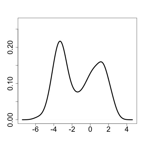
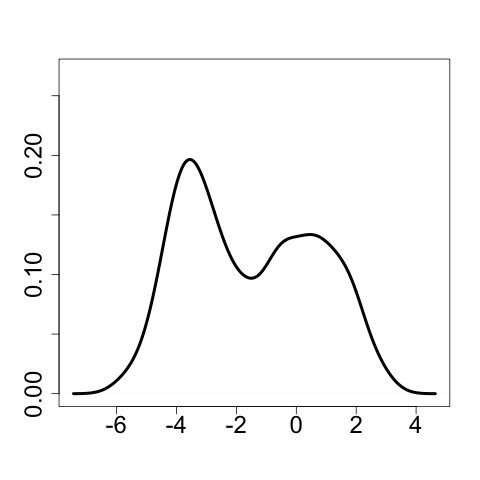
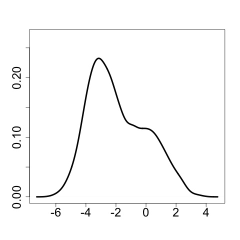
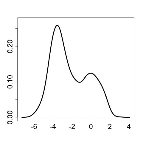
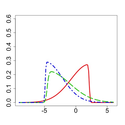
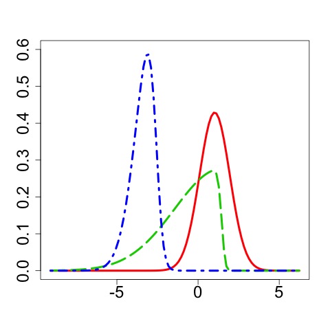
In this Section we apply our proposal on a real dataset, taken from the movebank website (van Bommel and Johnson, 2014a).

5.1 Data description

Data on free-ranging Maremma sheepdogs positions are recorded by tracking collars every 30 minutes. The behaviour of the dogs is unknown because there is minimal supervision by their owners and the animals are allowed to range freely. The dataset was first analyzed in van Bommel and Johnson (2014b) with the aim to understand how much space the dogs utilize and the portion of time that the dogs spent with livestock. Even if the primary purpose was not to identify behavioural modes, van Bommel and Johnson (2014b) results show that the dogs can be clustered in two states, one characterized by low speeds and tortuous path at the core of their home ranges (we call it state VB1), when they are resting or attending livestock, and large step-lengths (i.e. high movement speeds) in relatively straight lines, related to boundary patrolling or seeing off predators (we call it state VB2), at the edge of their home ranges.

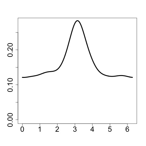
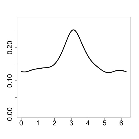
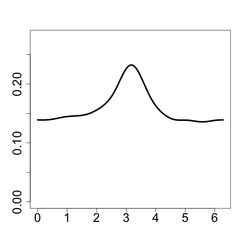
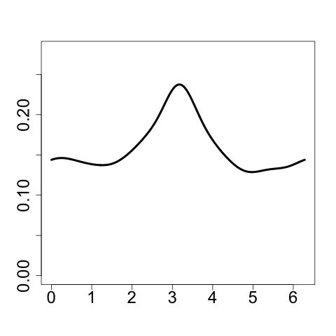
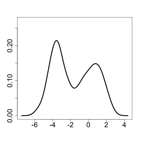
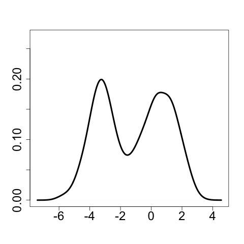
We characterize the hidden behaviours by analyzing the turning-angles and the logarithm of the step-lengths (log-step-lengths) for each dog taken into consideration. We model movement metrics belonging to dogs sharing the same property and observed on a common time period. We select the data from the “Heatherlie” property where between the 08/02/2012 5:30 and 10/03/2012 17:00, six dogs are observed, having then a time series of 3000 points with 6 circular and 6 linear variables. The six dogs have respectively 107, 63, 231, 43, 31 and 63 missing circular observations and 95, 53, 117, 32, 22 and 45 linear ones. The density estimates of the turning-angles and log-step-lengths can be seen in Figures 1 and 2. In the selected property and observational interval, van Bommel and Johnson (2014b) note that four of the six dogs form one social group responsible for protecting all livestock, one dog is old and mostly solitary and the last one suffers of an extreme social exclusion which severely restrict its movements. The animals that are part of the social group are often found together, but regularly they split into sub-groups.

5.2 Results

	1	2	3
1	0.711	0.181	0.108
	(0.679 0.741)	(0.154 0.209)	(0.085 0.132)
2	0.141	0.672	0.187
	(0.121 0.164)	(0.640 0.704)	(0.161 0.215)
3	0.083	0.209	0.708
	(0.065 0.103)	(0.180 0.239)	(0.676 0.739)

Table 1: Posterior mean estimates and 95 % credible intervals for the transition probability matrix: $\hat{K}=3$.

The model is estimated considering 400000 iterations, burnin 300000, thin 20 and by taking 5000 samples for inferential purposes. As prior distributions we choose $\boldsymbol{\mu}_{k},\boldsymbol{\Sigma}_{k}\sim NIW\left(\mathbf{0}_{6},0.001,25,\mathbf{I}_{6}\right)$ and $\boldsymbol{\lambda}_{k}\sim N_{2}\left(\mathbf{0}_{2},50\mathbf{I}_{2}\right)$ that are standard weak informative distributions. For the parameter $\rho$, that governs the self-transition probabilities, we decide to use $\rho\sim B(1,1)$, that is equivalent to a uniform distribution over $[0,1]$, while $\tau\sim G(1,0.01)$ and $\gamma\sim G(1,0.01)$. The priors of $\rho$, $\tau$ and $\gamma$ induce a prior over $K$ (Fox et al., 2011) that we evaluated through simulation, by using the degree $\ell$ weak limit approximation (Ishwaran and Zarepour, 2002) with $\ell=1000$; we found that ${K}\in[4,465]$ with a coverage of 95%.

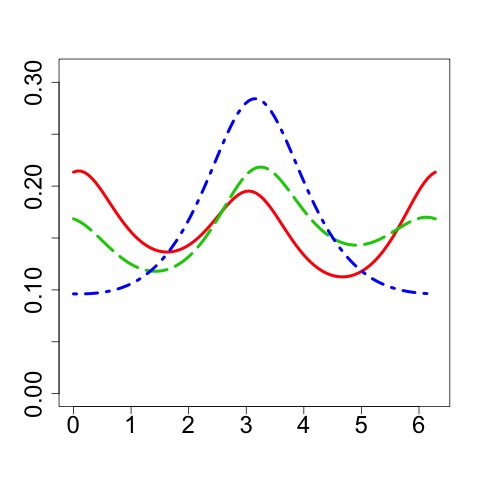
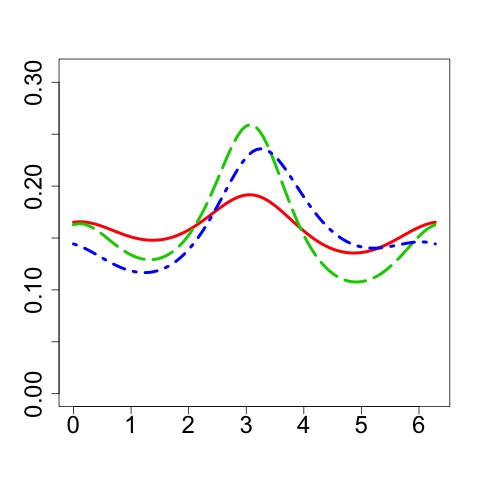
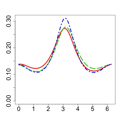
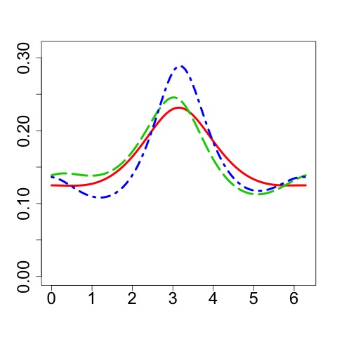
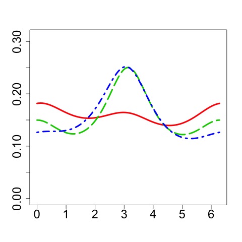
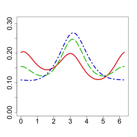
The model estimates 3 behavioural modes with $P(K=3|\boldsymbol{\theta},\mathbf{y})=1$. From the analysis of the posterior marginal distributions, Figures 3 and 4, and the correlation matrices $\boldsymbol{\Omega}_{k}$, Figure 5, we can easily interpret the behaviour modes, we can confirm what van Bommel and Johnson (2014b) found, we find connections between our estimated behavioural modes and the states VB1 and VB2 hypothesized by van Bommel and Johnson (2014b), and we add some new results. There are three groups of dogs that share similar marginal distributions: the dogs group one (DG1) composed by the dogs three and four, Figure 3 (c) and (d) and Figure 4 (c) and (d), the dog group two (DG2) is composed by the dogs two and five, Figure 3 (b) and (e) and Figure 4 (d) and (e), and the dogs one and six form the third group (DG3), Figure 3 (a) and (f) and Figure 4 (a) and (f).

In the first behaviour, all the dogs are in state VB1. They have small log-step-lengths and there are few movements in a straight line, i.e. the circular densities have low values at 0. There are few correlations that differ significantly from 0, see Figure 5 (a), and they have all mean posterior values (PEs) below 0.5. The stronger correlation (PE 0.474) is between the linear variables of the first and sixth dogs, i.e. the one in the DG3.

In the second behaviour, the linear distributions of the dogs in the DG3 have more mass of probability at higher values, but still having mass at low ones, and the correlation between the log-step-lengths increases (PE 0.840). The dogs in the DG3 have more movements in a straight line. The linear and circular distributions of the dogs in the DG1 and DG2 are similar to the ones of the first behaviour. The log-step-length of the dog two is correlated with the one of the dog three (PE 0.568) and five (PE 0.757) and the linear variables of the dogs five and six are correlated with PE 0.450. In this behaviour the dogs in the DG3 move to the state VB2 while the ones of the DG1 and DG2 remain in the state VB1.

In the third behaviour the linear distributions of the dogs in the DG3 put all the mass of probability on high values and the circular distributions have two modes, with more or less the same heights, at about 0 and $3.141$. The correlation between the linear variables of the dogs in the DG3 increases, with respect to the second behaviour, and it is almost one (PE 0.982). The two dogs change direction one accordingly to the other, since the cosine and sine of the circular variables are highly correlated (PEs 0.958 and 0.916). The linear distributions of the dogs in the DG2 move their mass of probability to higher values and the distributions resemble the ones of the dogs in the DG3, second behaviour. The circular distributions of the dogs in the DG2 are close to the circular uniform. The circular and linear distributions of the dogs in the DG1 are similar to the one of the first and second behaviours but their linear variables are now correlated (PE 0.781). In this behaviour the dogs in the DG3 remain in the state VB2 but, with respect to the second behaviour, they increase the amount of movement (in terms of higher step-length and more tortuous path). The dogs in the DG2 are in the state VB2 while the one in the DG1 remain in the state VB1. The dogs in the DG2 and DG3 have all the linear variables correlated.

The fourth dog is the one that suffers of an extreme social exclusion since its variables (circular and linear) are never correlated with the ones of the other dogs, with the exception of the third. The third dog is, probably, the old one since it does not move a lot, see Figure 4 (c), it is solitary, i.e. it bonds (in terms of correlation) only with the socially excluded one and, occasionally, with the dog two (second behaviour). The dogs in the DG2 and DG3 form one social group in the third behaviour, i.e. all the linear variables are correlated, and they split into subgroup in the behaviours one and two.

From Table 1 we see that there is a strong self-transition in all three behaviours (respectively PE 0.711, 0.672 and 0.708). The CIs of the probabilities to move to a new empty behaviour $\left(\sum_{k=4}^{\infty}\pi_{jk},\,j=1,2,3\right)$, not shown in Table 1, have always right side limit below 0.00001.

5.3 Comparisons with other emission distributions

	JPSN	VMLG	VMLW	WCLG	WCLW
$\hat{K}$	3	14	14	14	13
$CRPSc$	0.489	0.491	0.499	0.492	0.501
$CRPSl$	2.342	2.782	3.225	2.466	2.965

Table 2: Estimated number of non-empty behaviours ($\hat{K}$), mean CRPS for circular ($CRPSc$) and linear ($CRPSl$) variables, for the five models based on the JPSN, VMLG, VMLW, WCLG and WCLW.

(a)

(b)

Figure 6: Posterior marginal densities of the turning-angle (a) and the log-step-length (b) of the first dog estimated with the emission distribution WCLG.

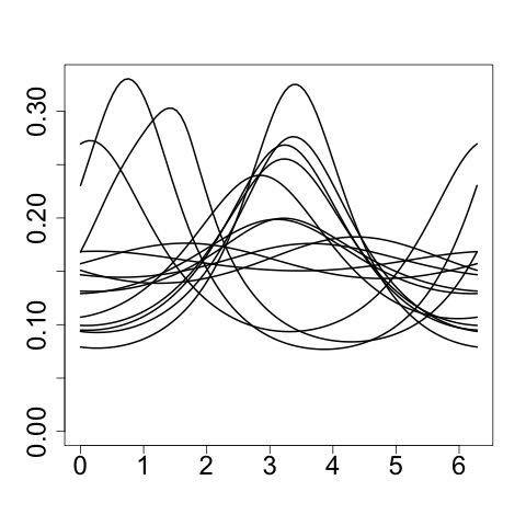
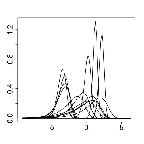
In this Section we show that our proposed emission distribution performs better, on the data we used in Section 5.2, than the standard distributions used in the literature. We are going to estimate sHDP-HMMs with different emission distributions and we compare the results. Unfortunately there are not measures of goodness of fit, such as the AIC or the BIC, when the model is based on the sHDP. Then we decide to base our comparison between models in terms of missing observations estimate, i.e. predictive ability, and behavioural modes interpretability.

To have a measure of how the model estimates the missing, we randomly select, for each circular and linear variables, 10% of the observations. We treat them as missing and, using the continuous ranked probability score (CRPS) (Matheson and Winkler, 1976), we compare the holdout values with the associated posterior distributions. The CRPS is a proper scoring rule that can be easily computed for both circular (Grimit et al., 2006) and linear (Gneiting and Raftery, 2007) variables using the MCMC output. Let $\mathcal{C}_{i}$ be the set of time points where the $i^{th}$ value of the circular variable is setted as missing, $\mathcal{L}_{j}$ be the ones of the $j^{th}$ linear variable and let $\theta_{ti}^{b}$, $t\in\mathcal{C}_{i}$ and $y_{tj}^{b}$, $t\in\mathcal{L}_{j}$ be respectively the $b^{th}$ posterior sample of $\theta_{ti}$ and $y_{tj}$. A Monte Carlo approximation of the CRPS for a circular variable is computed as

$$CRPSc_{i}\approx\frac{1}{B}\sum_{b=1}^{B}d(\theta_{ti},\theta_{ti}^{b})-\frac{1}{2B^{2}}\sum_{b=1}^{B}\sum_{b^{\prime}=1}^{B}d(\theta_{ti}^{b},\theta_{ti}^{b^{\prime}}),\,t\in\mathcal{C}_{i},$$ (27)

where $d(\cdot,\cdot)$ is the angular distance. The CRPS for a linear variable is approximated with

$$CRPSl_{j}\approx\frac{1}{B}\sum_{b=1}^{B}|y_{tj}-y_{tj}^{b}|-\frac{1}{2B^{2}}\sum_{b=1}^{B}\sum_{b^{\prime}=1}^{B}|y_{tj}^{b}-y_{tj}^{b^{\prime}}|,\,t\in\mathcal{L}_{j}.$$ (28)

We then compute the overall mean CRPS for the circular variables, $CRPSc=\frac{1}{n}\sum_{i=1}^{n}CRPSc_{i}$, and the linear ones, $CRPSl=\frac{1}{q}\sum_{j=1}^{q}CRPSl_{j}$, and we use these two indeces to measure the ability of the model in estimating the missing observations.

It is generally supposed, in the literature, that the turning-angle is distributed as a von Mises (Langrock et al., 2012; Holzmann et al., 2006; Eckert et al., 2008) or a wrapped Cauchy (Langrock et al., 2012; Eckert et al., 2008; Morales et al., 2004; Holzmann et al., 2006) while the gamma (Langrock et al., 2012; Holzmann et al., 2006) or the Weibull (Langrock et al., 2012; Morales et al., 2004) are used for the step-length; these distributions are compared with our proposal. In the model specification, Section 4.1, we assume that each linear variable belongs to $\mathbb{R}$ and then, instead of the gamma and Weibull, we use the log-gamma and log-Weibull, i.e. the distributions that arise by taking the log of, respectively, a random variable gamma or Weibull distributed. The model in Section 4 is compared with the ones based on the von Mises and the log-gamma (VMLG), the von Mises and the log-Weibull (VMLW), the wrapped Cauchy and the log-gamma (WCLG), the wrapped Cauchy and the log-Weibull (WCLW). There is not an obvious way to introduce dependence between the movement metrics on the model VMLG, VMLW, WCLG and WCLW, and, in the literature, they are generally supposed to be independent (see for example Morales et al. (2004) or Langrock et al. (2012)). Then, in these models, we assume the following:

$$f(\boldsymbol{\theta},\mathbf{y}|\{z_{t}\}_{t\in\mathcal{T}}\{\boldsymbol{\psi}_{k}\}_{k\in\mathcal{K}})=\prod_{t\in\mathcal{T}}\prod_{k\in\mathcal{K}}\left[\prod_{i=1}^{n}f(\theta_{ti}|\boldsymbol{\psi}_{z_{t}})\prod_{j=1}^{q}f(y_{tj}|\boldsymbol{\psi}_{z_{t}})\right]^{I(z_{t},k)}.$$ (29)

We use a $G(1,0.5)$ as prior for the shape and rate parameters of the log-gamma and the log-Weibull, that is a standard weak-informative prior. For the two parameters of the wrapped Cauchy, one defined over $[0,2\pi)$ and one over $[0,1]$, we use uniform distributions in the respective domains while on the two parameters of the von Mises, one defined over $[0,2\pi)$ and one over $\mathbb{R}^{+}$, we use respectively the non-informative $U(0,2\pi)$ and the weak informative $G(1,0.5)$. As prior distributions for the sHDP parameters, we use the same used in Section 5.

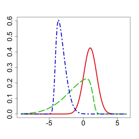
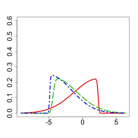
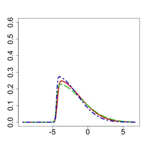
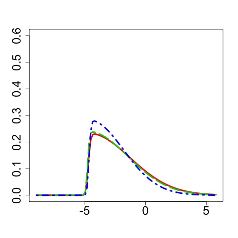
In Table 2 we can see the estimated number of non-empty behaviours $(\hat{K})$, $CRPSc$s and $CRPSl$s. The predictive ability of our model outperforms all the others in both CRPS for circular and linear variables. The models based on the VMLG, VMLW, WCLG and WCLW estimate a larger number of behaviours, with respect to our proposal, i.e. in three of them $\hat{K}=$14 and in one $\hat{K}=$13; we can see an example of the estimated behaviours in Figure 6. It is challenging to give an interpretation to these behaviours and moreover such a large number of behaviours does not increase the predictive ability of the models, see Table 2.

A possible explanation of why the models based on the VMLG, VMLW, WCLG and WCLW estimate 13 or 14 behaviours can be found in Mastrantonio et al. (2015a). They simulate datasets using bivariate emission distributions with dependent components, bimodal marginals for the circular variable, with the aim to understand what happens if, on the simulated datasets, are estimated HMMs with emission distributions that do not allow for dependent components and bimodality in the circular marginal. They found that the number of behaviours is generally overestimated, since each behaviour is separated into two, one for each mode of the circular distribution.
In our real data application, we have six circular and six linear variables, some of them are correlated and often the marginal circular distributions have two modes, see Figure 3. If we assume independence between the circular and linear variables, as we did in the model base on the VMLG, VMLW, WCLG and WCLW, and the marginal circular distributions are unimodal, as the von Mises and the wrapped Cauchy, then we can expect a large number of behaviours.

6 Conclusions

The primary objective of this work, motivated by our real data, was to introduce an HMM capable of modelling a group of animals, taking into account possible correlations between the associated movement metrics. For this reason we introduced a new multivariate circular-linear distribution, namely the JPSN. The new distribution has dependent components and it is used as emission distribution in the HMM. The HMM was estimated under a non-parametric Bayesian framework and we showed how to implement the MCMC algorithm.

The model, applied to the real data example, confirmed known results and added new ones. We showed that our emission distribution outperforms the most used in the literature in terms of predictive ability and the estimated behaviours are more easily interpretable.

Future work will lead us to incorporate covariates to model the circular-linear mean and variance of the JPSN and we will explore different temporal dependence structures, such as the semi-HMM or the autoregressive-HMM.

References

- Abe and Ley (2015) Abe, T. and Ley, C. (2015). A tractable, parsimonious and highly flexible model for cylindrical data, with applications. ArXiv e-prints.
- Arellano-Valle et al. (2007) Arellano-Valle, R., Bolfarine, H., and Lachos, V. (2007). Bayesian inference for skew-normal linear mixed models. Journal of Applied Statistics, 34(6), 663–682.
- Blackwell (2003) Blackwell, P. G. (2003). Bayesian inference for markov processes with diffusion and discrete components. Biometrika, 90(3), 613–627.
- Brownlee (1912) Brownlee, J. (1912). The mathematical theory of random migration and epidemic distribution. Proceedings of the Royal Society of Edinburgh, 31, 262–289.
- Cagnacci et al. (2010) Cagnacci, F., Boitani, L., Powell, R. A., and Boyce, M. S. (2010). Animal ecology meets gps-based radiotelemetry: a perfect storm of opportunities and challenges. Philosophical Transactions of the Royal Society of London B: Biological Sciences, 365(1550), 2157–2162.
- Cappé et al. (2005) Cappé, O., Moulines, E., and Ryden, T. (2005). Inference in Hidden Markov Models. Springer Series in Statistics. Springer.
- Ciucci et al. (2009) Ciucci, P., Reggioni, W., Maiorano, L., and Boitani, L. (2009). Long-distance dispersal of a rescued wolf from the northern apennines to the western alps. The Journal of Wildlife Management, 73(8), 1300–1306.
- D’Elia (2001) D’Elia, A. (2001). A statistical model for orientation mechanism. Statistical Methods and Applications, 10(1-3), 157–174.
- Eckert et al. (2008) Eckert, S. A., Moore, J. E., Dunn, D. C., van Buiten, R. S., Eckert, K. L., and Halpin, P. N. (2008). Modeling loggerhead turtle movement in the mediterranean: importance of body size and oceanography. Ecological Applications, 18(2), 290–308.
- Fox et al. (2011) Fox, E. B., Sudderth, E. B., Jordan, M. I., and Willsky, A. S. (2011). A sticky hdp-hmm with application to speaker diarization. The Annals of Applied Statistics, 5(2A), 1020–1056.
- Franke et al. (2004) Franke, A., Caelli, T., and Hudson, R. J. (2004). Analysis of movements and behavior of caribou (rangifer tarandus) using hidden markov models. Ecological Modelling, 173(2â3), 259 – 270.
- Gneiting and Raftery (2007) Gneiting, T. and Raftery, A. E. (2007). Strictly proper scoring rules, prediction, and estimation. Journal of the American Statistical Association, 102(477), 359–378.
- Green (1995) Green, P. J. (1995). Reversible jump Markov chain monte carlo computation and Bayesian model determination. Biometrika, 82(4), 711–732.
- Grimit et al. (2006) Grimit, E. P., Gneiting, T., Berrocal, V. J., and Johnson, N. A. (2006). The continuous ranked probability score for circular variables and its application to mesoscale forecast ensemble verification. Quarterly Journal of the Royal Meteorological Society, 132(621C), 2925–2942.
- Hanks et al. (2015) Hanks, E. M., Hooten, M. B., and Alldredge, M. W. (2015). Continuous-time discrete-space models for animal movement. Ann. Appl. Stat., 9(1), 145–165.
- Holzmann et al. (2006) Holzmann, H., Munk, A., Suster, M., and Zucchini, W. (2006). Hidden Markov models for circular and linear-circular time series. Environmental and Ecological Statistics, 13(3), 325–347.
- Hooten et al. (2010) Hooten, M., Johnson, D., Hanks, E., and Lowry, J. (2010). Agent-based inference for animal movement and selection. Journal of Agricultural, Biological, and Environmental Statistics, 15(4), 523–538.
- Horne et al. (2007) Horne, J. S., Garton, E. O., Krone, S. M., and Lewis, J. S. (2007). Analyzing animal movements using brownian brigdes. Ecology, 88(9), 2354–2363.
- Houston and Mcnamara (1999) Houston, A. I. and Mcnamara, J. M. (1999). Models of Adaptive Behaviour: An approach based on state. Cambridge University Press, Cambridge, United Kingdom.
- Huang and Wand (2013) Huang, A. and Wand, M. P. (2013). Simple marginally noninformative prior distributions for covariance matrices. Bayesian Analysis, 1, 1–14.
- Ishwaran and Zarepour (2002) Ishwaran, H. and Zarepour, M. (2002). Exact and approximate sum representations for the dirichlet process. Canadian Journal of Statistics, 30(2), 269–283.
- Jammalamadaka and SenGupta (2001) Jammalamadaka, S. R. and SenGupta, A. (2001). Topics in Circular Statistics. World Scientific, Singapore.
- Jonsen et al. (2005) Jonsen, I. D., Flemming, J. M., and Myers, R. A. (2005). Robust state-space modeling of animal movement data. Ecology, 86(11), 2874–2880.
- Jonsen et al. (2006) Jonsen, I. D., Myers, R. A., and James, M. C. (2006). Robust hierarchical state-space models reveal diel variation in travel rates of migrating leatherback turtles. Journal of Animal Ecology, 75(5), 1046–1057.
- Jonsen et al. (2007) Jonsen, I. D., Myers, R. A., and James, M. C. (2007). Identifying leatherback turtle foraging behaviour from satellite telemetry using a switching state-space model. Marine Ecology Progress Series, 337, 255–264.
- Langrock et al. (2012) Langrock, R., King, R., Matthiopoulos, J., Thomas, L., Fortin, D., and Morales, J. M. (2012). Flexible and practical modeling of animal telemetry data: hidden Markov models and extensions. Ecology, 93(11), 2336–2342.
- Langrock et al. (2014) Langrock, R., Hopcraft, G., Blackwell, P., Goodall, V., King, R., Niu, M., Patterson, T., Pedersen, M., Skarin, A., and Schick, R. (2014). Modelling group dynamic animal movement. Methods in Ecology and Evolution, 5(2), 190–199.
- Mardia and Jupp (1999) Mardia, K. V. and Jupp, P. E. (1999). Directional Statistics. John Wiley and Sons, Chichester.
- Mastrantonio et al. (2015a) Mastrantonio, G., Maruotti, A., and Jona Lasinio, G. (2015a). Bayesian hidden markov modelling using circular-linear general projected normal distribution. Environmetrics, 26, 145–158.
- Mastrantonio et al. (2015b) Mastrantonio, G., Jona Lasinio, G., and Gelfand, A. E. (2015b). Spatio-temporal circular models with non-separable covariance structure. TEST, To appear.
- Matheson and Winkler (1976) Matheson, J. E. and Winkler, R. L. (1976). Scoring rules for continuous probability distributions. Management Science, 22(10), 1087–1096.
- McClintock et al. (2012) McClintock, B. T., King, R., Thomas, L., Matthiopoulos, J., McConnell, B. J., and Morales, J. M. (2012). A general discrete-time modeling framework for animal movement using multistate random walks. Ecological Monographs, 82(3), 335–349.
- Morales et al. (2004) Morales, J. M., Haydon, D. T., Frair, J., Holsinger, K. E., and Fryxell, J. M. (2004). Extracting more out of relocation data: building movement models as mixtures of random walks. Ecology, 85(9), 2436–2445.
- Morales et al. (2010) Morales, J. M., Moorcroft, P. R., Matthiopoulos, J., Frair, J. L., Kie, J. G., Powell, R. A., Merrill, E. H., and Haydon, D. T. (2010). Building the bridge between animal movement and population dynamics. Philosophical Transactions of the Royal Society B: Biological Sciences, 365(1550), 2289–2301.
- O’Malley and Zaslavsky (2008) O’Malley, A. J. and Zaslavsky, A. M. (2008). Domain-level covariance analysis for multilevel survey data with structured nonresponse. Journal of the American Statistical Association, 103(484), 1405–1418.
- Patterson et al. (2008) Patterson, T., Thomas, L., Wilcox, C., Ovaskainen, O., and Matthiopoulos, J. (2008). State-space models of individual animal movement. Trends in Ecology & Evolution, 23(2), 87–94.
- Patterson et al. (2009) Patterson, T. A., Basson, M., Bravington, M. V., and Gunn, J. S. (2009). Classifying movement behaviour in relation to environmental conditions using hidden markov models. Journal of Animal Ecology, 78(6), 1113–1123.
- Sahu et al. (2003) Sahu, S. K., Dey, D. K., and Branco, M. D. (2003). A new class of multivariate skew distributions with applications to Bayesian regression models. Canadian Journal of Statistics, 31(2), 129–150.
- Schliehe-Diecks et al. (2012) Schliehe-Diecks, S., Kappeler, P. M., and Langrock, R. (2012). On the application of mixed hidden markov models to multiple behavioural time series. Interface Focus, 2(2), 180–189.
- SenGupta (2004) SenGupta, A. (2004). On the construction of probability distributions for directional data. Bulletin of Calcutta Mathematical Society, 96, 139–154.
- Sengupta and Ong (2014) Sengupta, A. and Ong, S. H. (2014). A unified approach for construction of probability models for bivariate linear and directional data. Communications in Statistics - Theory and Methods, 43(10-12), 2563–2569.
- Sethuraman (1994) Sethuraman, J. (1994). A constructive definition of Dirichlet priors. Statistica Sinica, 4, 639–650.
- Teh et al. (2006) Teh, Y. W., Jordan, M. I., Beal, M. J., and Blei, D. M. (2006). Hierarchical dirichlet processes. Journal of the American Statistical Association, 101(476), 1566–1581.
- van Bommel and Johnson (2014a) van Bommel, L. and Johnson, C. (2014a). Data from: Where do livestock guardian dogs go? movement patterns of free-ranging maremma sheepdogs. movebank data repository.
- van Bommel and Johnson (2014b) van Bommel, L. and Johnson, C. (2014b). Where do livestock guardian dogs go? movement patterns of free-ranging maremma sheepdogs. PLoS ONE, 9(10).
- Van Gael et al. (2008) Van Gael, J., Saatci, Y., Teh, Y. W., and Ghahramani, Z. (2008). Beam sampling for the infinite hidden Markov model. In Proceedings of the 25th International Conference on Machine Learning, ICML ’08, pages 1088–1095, New York, NY, USA. ACM.
- Wang and Gelfand (2013) Wang, F. and Gelfand, A. E. (2013). Directional data analysis under the general projected normal distribution. Statistical Methodology, 10(1), 113–127.
- Wang and Gelfand (2014) Wang, F. and Gelfand, A. E. (2014). Modeling space and space-time directional data using projected Gaussian processes. Journal of the American Statistical Association, 109(508), 1565–1580.