Convergent Learning: Do different neural networks learn the same representations?
Abstract
Recent successes in training large, deep neural networks have prompted active investigation into the representations learned on their intermediate layers. Such research is difficult because it requires making sense of non-linear computations performed by millions of learned parameters, but valuable because it increases our ability to understand current models and training algorithms and thus create improved versions of them. In this paper we investigate the extent to which neural networks exhibit what we call convergent learning, which is when the representations learned by multiple nets converge to a set of features which are either individually similar between networks or where subsets of features span similar low-dimensional spaces. We propose a specific method of probing representations: training multiple networks and then comparing and contrasting their individual, learned representations at the level of neurons or groups of neurons. We begin research into this question by introducing three techniques to approximately align different neural networks on a feature or subspace level: a bipartite matching approach that makes one-to-one assignments between neurons, a sparse prediction and clustering approach that finds one-to-many mappings, and a spectral clustering approach that finds many-to-many mappings. This initial investigation reveals a few interesting, previously unknown properties of neural networks, and we argue that future research into the question of convergent learning will yield many more. The insights described here include (1) that some features are learned reliably in multiple networks, yet other features are not consistently learned; (2) that units learn to span low-dimensional subspaces and, while these subspaces are common to multiple networks, the specific basis vectors learned are not; (3) that the representation codes show evidence of being a mix between a local (single unit) code and slightly, but not fully, distributed codes across multiple units; (4) that the average activation values of neurons vary considerably within a network, yet the mean activation values across different networks converge to an almost identical distribution. 111A preliminary version of this work was presented at the NIPS 2015 Feature Extraction workshop.
1 Introduction
Many recent studies have focused on understanding deep neural networks from both a theoretical perspective (Arora et al., 2014; Neyshabur & Panigrahy, 2013; Montavon et al., 2011; Paul & Venkatasubramanian, 2014; Goodfellow et al., 2014) and from an empirical perspective (Erhan et al., 2009; Eigen et al., 2013; Szegedy et al., 2013; Simonyan et al., 2013; Zeiler & Fergus, 2014; Nguyen et al., 2014; Yosinski et al., 2014; Mahendran & Vedaldi, 2014; Yosinski et al., 2015; Zhou et al., 2014). In this paper we continue this trajectory toward attaining a deeper understanding of neural net training by proposing a new approach. We begin by noting that modern deep neural networks (DNNs) exhibit an interesting phenomenon: networks trained starting at different random initializations frequently converge to solutions with similar performance (see Dauphin et al. (2014) and Section 2 below). Such similar performance by different networks raises the question of to what extent the learned internal representations differ: Do the networks learn radically different sets of features that happen to perform similarly, or do they exhibit convergent learning, meaning that their learned feature representations are largely the same? This paper makes a first attempt at asking and answering these questions. Any improved understanding of what neural networks learn should improve our ability to design better architectures, learning algorithms, and hyperparameters, ultimately enabling more capable models. For instance, distributed data-parallel neural network training is more complicated than distributed data-parallel training of convex models because periodic direct averaging of model parameters is not an effective strategy: perhaps solving a neuron correspondence problem before averaging would mitigate the need for constant synchronization. As another example, if networks converge to diverse solutions, then perhaps additional performance improvements are possible via training multiple models and then using model compilation techniques to realize the resulting ensemble in a single model.
In this paper, we investigate the similarities and differences between the representations learned by neural networks with the same architecture trained from different random initializations. We employ an architecture derived from AlexNet (Krizhevsky et al., 2012) and train multiple networks on the ImageNet dataset (Deng et al., 2009) (details in Section 2). We then compare the representations learned across different networks. We demonstrate the effectiveness of this method by both visually and quantitatively showing that the features learned by some neuron clusters in one network can be quite similar to those learned by neuron clusters in an independently trained neural network. Our specific contributions are asking and shedding light on the following questions:
-
1.
By defining a measure of similarity between units222Note that we use the words “filters”, “channels”, “neurons”, and “units” interchangeably to mean channels for a convolutional layer or individual units in a fully connected layer. in different neural networks, can we come up with a permutation for the units of one network to bring it into a one-to-one alignment with the units of another network trained on the same task? Is this matching or alignment close, because features learned by one network are learned nearly identically somewhere on the same layer of the second network, or is the approach ill-fated, because the representations of each network are unique? (Answer: a core representation is shared, but some rare features are learned in one network but not another; see Section 3).
-
2.
Are the above one-to-one alignment results robust with respect to different measures of neuron similarity? (Answer: yes, under both linear correlation and estimated mutual information metrics; see Section 3.2).
-
3.
To the extent that an accurate one-to-one neuron alignment is not possible, is it simply because one network’s representation space is a rotated version333Or, more generally, a space that is an affine transformation of the first network’s representation space. of another’s? If so, can we find and characterize these rotations? (Answers: by learning a sparse weight LASSO model to predict one representation from only a few units of the other, we can see that the transform from one space to the other can be possibly decoupled into transforms between small subspaces; see Section 4).
-
4.
Can we further cluster groups of neurons from one network with a similar group from another network? (Answer: yes. To approximately match clusters, we adopt a spectral clustering algorithm that enables many-to-many mappings to be found between networks. See Section S.3).
-
5.
For two neurons detecting similar patterns, are the activation statistics similar as well? (Answer: mostly, but with some differences; see Section S.4).
2 Experimental Setup
All networks in this study follow the basic architecture laid out by Krizhevsky et al. (2012), with parameters learned in five convolutional layers ( – ) followed by three fully connected layers ( – ). The structure is modified slightly in two ways. First, Krizhevsky et al. (2012) employed limited connectivity between certain pairs of layers to enable splitting the model across two GPUs.444In Krizhevsky et al. (2012) the , , and layers were only connected to half of the preceding layer’s channels. Here we remove this artificial group structure and allow all channels on each layer to connect to all channels on the preceding layer, as we wish to study only the group structure, if any, that arises naturally, not that which is created by architectural choices. Second, we place the local response normalization layers after the pooling layers following the defaults released with the Caffe framework, which does not significantly impact performance (Jia et al., 2014). Networks are trained using Caffe on the ImageNet Large Scale Visual Recognition Challenge (ILSVRC) 2012 dataset (Deng et al., 2009). Further details and the complete code necessary to reproduce these experiments is available at https://github.com/yixuanli/convergent_learning.
We trained four networks in the above manner using four different random initializations. We refer to these as , , , and . The four networks perform very similarly on the validation set, achieving top-1 accuracies of 58.65%, 58.73%, 58.79%, and 58.84%, which are similar to the top-1 performance of 59.3% reported in the original study (Krizhevsky et al., 2012).
We then aggregate certain statistics of the activations within the networks. Given a network trained in this manner, the scalar random variable denotes the series of activation values produced over the entire ILSVRC validation dataset by unit on layer .555 For the fully connected layers, the random variable has one specific value for each input image; for the convolutional layers, the value of takes on different values at each spatial position. In other words, to sample an for an FC layer, we pick a random image from the validation set; to sample for a conv layer, we sample a random image and a random position within the conv layer. We collect the following statistics by aggregating over the validation set (and in the case of convolutional layers also over spatial positions):
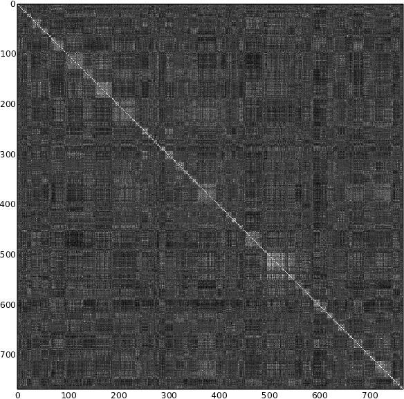
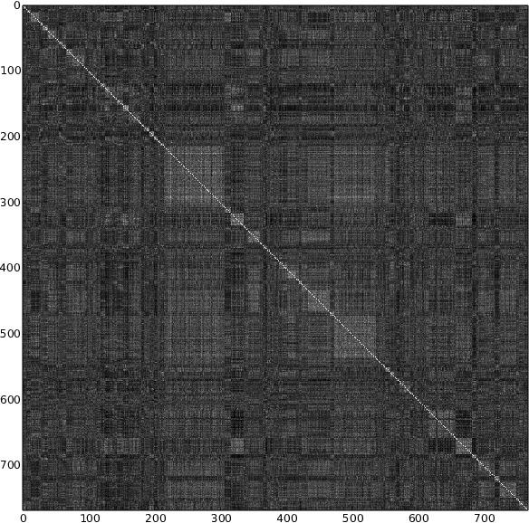
Intuitively, we compute the mean and standard deviation of the activation of each unit in the network over the validation set. For convolutional layers, we compute the mean and standard deviation of each channel. The mean and standard deviation for a given network and layer is a vector with length equal to the number of channels (for convolutional layers) or units (for fully connected layers).666 For reference, the number of channels for to is given by: . The corresponding size of the correlation matrix in each layer is: . Furthermore, the spatial extents of each channel in each convolutional layer is given by: The within-net correlation values for each layer can be considered as a symmetric square matrix with side length equal to the number of units in that layer (e.g. a matrix for as in Figure 1a,b). For a pair of networks, the between-net correlation values also form a square matrix, which in this case is not symmetric (Figure 1c,d).

(a) (b) (c) (d)
We use these correlation values as a way of measuring how related the activations of one unit are to another unit, either within the network or between networks. We use correlation to measure similarity because it is independent of the scale of the activations of units. Within-net correlation quantifies the similarity between two neurons in the same network; whereas the between-net correlation matrix quantifies the similarity of two neurons from different neural networks. Note that the units compared are always on the same layer on the network; we do not compare units between different layers. In the Supplementary Information (see Figure S1), we plot the activation values for several example high correlation and low correlation pairs of units from and layers; the simplicity of the distribution of values suggests that the correlation measurement is an adequate indicator of the similarity between two neurons. To further confirm this suspicion, we also tested with a full estimate of the mutual information between units and found it to yield similar results to correlation (see Section 3.2).
3 Is There a One-to-One Alignment Between Features Learned by Different Neural Networks?
We would like to investigate the similarities and differences between multiple training runs of same network architecture. Due to symmetries in the architecture and weight initialization procedures, for any given parameter vector that is found, one could create many equivalent solutions simply by permuting the unit orders within a layer (and permuting the outgoing weights accordingly). Thus, as a first step toward analyzing the similarities and differences between different networks, we ask the following question: if we allow ourselves to permute the units of one network, to what extent can we bring it into alignment with another? To do so requires finding equivalent or nearly-equivalent units across networks, and for this task we adopt the magnitude independent measures of correlation and mutual information. We primarily give results with the simpler, computationally faster correlation measure (Section 3.1), but then confirm the mutual information measure provides qualitatively similar results (Section 3.2).
3.1 Alignment via Correlation
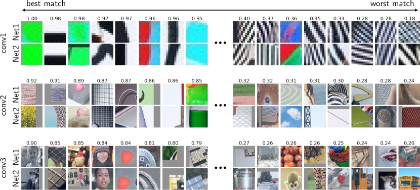
As discussed in Section 2, we compute within-net and between-net unit correlations. Figure 1 shows the within-net correlation values computed between units on a network and other units on the same network (panels a,b) as well as the between-net correlations between two different networks (panel c). We find matching units between a pair of networks — here and — in two ways. In the first approach, for each unit in , we find the unit in with maximum correlation to it, which is the max along each row of Figure 1c. This type of assignment is known as a bipartite semi-matching in graph theory (Lawler, 1976), and we adopt the same nomenclature here. This procedure can result in multiple units of being paired with the same unit in . Figure 2 shows the eight highest correlation matched features and eight lowest correlation matched features using the semi-matching approach (corresponding to the leftmost eight and rightmost eight points in Figure 3.1). To visualize the functionality each unit, we plot the image patch from the validation set that causes the highest activation for that unit. For all the layers shown, the most correlated filters (on the left) reveal that there are nearly perfect counterparts in each network, whereas the low-correlation filters (on the right) reveal that there are many features learned by one network that are unique and thus have no corollary in the other network.
An alternative approach is to find the one-to-one assignment between units in and without replacement, such that every unit in each network is paired with a unique unit in the other network. This more common approach is known as bipartite matching.777Note that the semi-matching is “row-wise greedy” and will always have equal or better sum of correlation than the matching, which maximizes the same objective but must also satisfy global constraints. A matching that maximizes the sum of the chosen correlation values may be found efficiently via the Hopcroft-Karp algorithm (Hopcroft & Karp, 1973) after turning the between-net correlation matrix into a weighted bipartite graph. Figure 1c shows an example between-net correlation matrix; the max weighted matching can be thought of as a path through the matrix such that each row and each column are selected exactly once, and the sum of elements along the path is maximized. Once such a path is found, we can permute the units of to bring it into the best possible alignment with , so that the first channel of approximately matches (has high correlation with) the first channel of , the second channels of each also approximately match, and so on. The correlation matrix of with the permuted version of is shown in Figure 1d. Whereas the diagonal of the self correlation matrices are exactly one, the diagonal of the permuted between-net correlation matrix contains values that are generally less than one. Note that the diagonal of the permuted between-net correlation matrix is bright (close to white) in many places, which shows that for many units in it is possible to find a unique, highly correlated unit in .
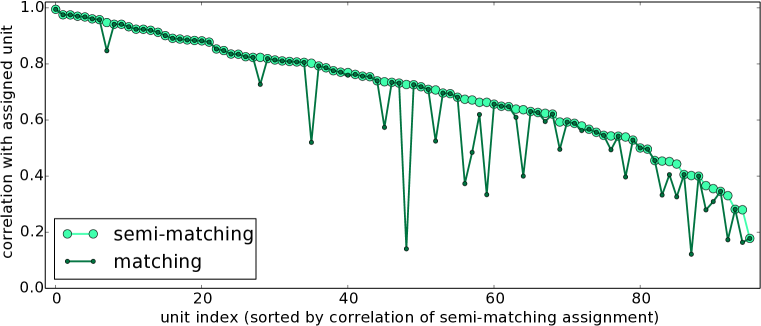
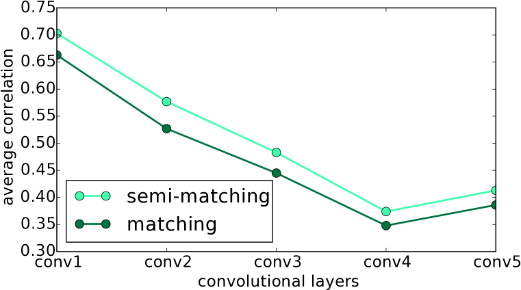
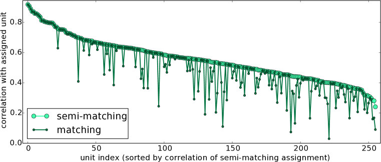
Figure 3.1 shows a comparison of assignments produced by the semi-matching and matching methods for the layer (Figure S3 shows results for other layers). Insights into the differing representations learned can be gained from both assignment methods. The first conclusion is that for most units, particularly those with the higher semi-matching and matching correlations (Figure 3.1, left), the semi-matching and matching assignments coincide, revealing that for many units a one-to-one assignment is possible. Both methods reveal that the average correlation for one-to-one alignments varies from layer to layer (Figure 3.1), with the highest matches in the and layers, but worse matches in between. This pattern implies that the path from a relatively matchable representation to representation passes through an intermediate middle region where matching is more difficult, suggesting that what is learned by different networks on and is more convergent than , and . This result may be related to previously observed greater complexity in the intermediate layers as measured through the lens of optimization difficulty (Yosinski et al., 2014).
Next, we can see that where the semi-matching and matching differ, the matching is often much worse.One hypothesis for why this occurs is that the two networks learn different numbers of units to span certain subspaces. For example, might learn a representation that uses six filters to span a subspace of human faces, but learns to span the same subspace with five filters. With unique matching, five out of the six filters from may be matched to their nearest counterpart in , but the sixth unit will be left without a counterpart and will end up paired with an almost unrelated filter.
Finally, with reference to Figure 3.1 (but similarly observable in Figure S3 for other layers), another salient observation is that the correlation of the semi-matching falls significantly from the best-matched unit (correlations near 1) to the lowest-matched (correlations near 0.3). This indicates that some filters in can be paired up with filters in with high correlation, but other filters in and are network-specific and have no high-correlation pairing in the alternate network, implying that those filters are rare and not always learned. This holds across the – layers.
3.2 Alignment via Mutual Information
Because correlation is a relatively simple mathematical metric that may miss some forms of statistical dependence, we also performed one-to-one alignments of neurons by measuring the mutual information between them. Mutual information measures how much knowledge one gains about one variable by knowing the value of another. Formally, the mutual information of the two random variables and representing the activation of the -th neuron in and the -th neuron in , is defined as:
where is the joint probability distribution of and , and and are their marginal probability distributions, respectively. The within-net mutual information matrix and between-net mutual information matrix have the same shapes as their equivalent correlation matrices.
We apply the same matching technique described in Section 3.1 to the between-net mutual information matrix,888The mutual information between each pair of neurons is estimated using 1D and 2D histograms of paired activation values over 60,000 random activation samples. We discretize the activation value distribution into percentile bins along each dimension, each of which captures 5% of the marginal distribution mass. We also add a special bin with range in order to capture the significant mass around 0. and compare the highest and lowest mutual information matches (Figure S4) to those obtained via correlation (Figure 2). The results are qualitatively the same. For example, seven out of eight best matched pairs in the layer stay the same. These results suggest that correlation is an adequate measurement of the similarity between two neurons, and that switching to a mutual information metric would not qualitatively change the correlation-based conclusions presented above.
4 Relaxing the One-to-One Constraint to Find Sparse, Few-to-One Mappings
The preceding section showed that, while some neurons have a one-to-one match in another network, for other neurons no one-to-one match exists (with correlation above some modest threshold). For example, 17% of neurons in have no match in with a correlation above (Figure 3.1); this number rises to 37% for , 63% for , and 92% for , before dropping to 75% for (see Figure S3).
These numbers indicate that, particularly for intermediate layers, a simple one-to-one mapping is not a sufficient model to predict the activations of some neurons in one network given the activations of neurons in another network (even with the same architecture trained on the same task). That result could either be because the representations are unique (i.e. not convergent), or because the best possible one-to-one mapping is insufficient to tell the complete story of how one representation is related to another. We can think of a one-to-one mapping as a model that predicts activations in the second network by multiplying the activations of the first by a permutation matrix — a square matrix constrained such that each row and each column contain a single one and the rest zeros. Can we do better if we learn a model without this constraint?
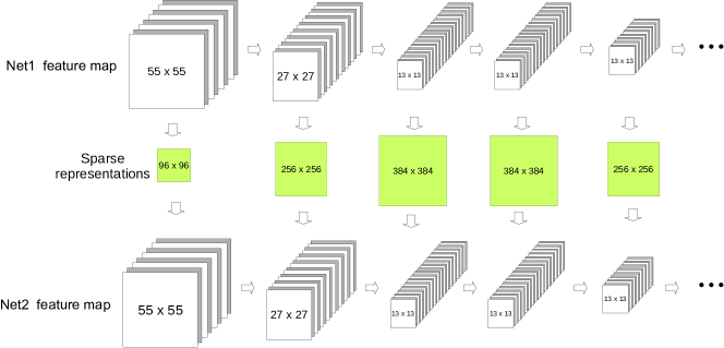
We can relax this one-to-one constraint to various degrees by learning a mapping layer with an L1 penalty (known as a LASSO model, (Tibshirani, 1996)), where stronger penalties will lead to sparser (more few-to-one or one-to-one) mappings. This sparsity pressure can be varied from quite strong (encouraging a mostly one-to-one mapping) all the way to zero, which encourages the learned linear model to be dense. More specifically, to predict one layer’s representation from another, we learn a single mapping layer from one to the other (similar to the “stitching layer” in Lenc & Vedaldi (2015)). In the case of convolutional layers, this mapping layer is a convolutional layer with kernel size and number of output channels equal to the number of input channels. The mapping layer’s parameters can be considered as a square weight matrix with side length equal to the number of units in the layer; the layer learns to predict any unit in one network via a linear weighted sum of any number of units in the other. The model and resulting square weight matrices are shown in Figure 5. This layer is then trained to minimize the sum of squared prediction errors plus an L1 penalty, the strength of which is varied.999Both representations (input and target) are taken after the relu is applied. Before training, each channel is normalized to have mean zero and standard deviation , where is the number of dimensions of the representation at that layer (e.g. for ). This normalization has two effects. First, the channels in a layer are all given equal importance, without which the channels with large activation values (see Figure S10) dominate the cost and are predicted well at the expense of less active channels, a solution which provides little information about the less active channels. Second, the representation at any layer for a single image becomes approximately unit length, making the initial cost about the same on all layers and allowing the same learning rate and SGD momentum hyperparameters to be used for all layers. It also makes the effect of specific L1 multipliers approximately commensurate and allows for rough comparison of prediction performance between layers, because the scale is constant.
| Sparse Prediction Loss (after 4,500 iterations) | ||||||
| decay 0 | decay | decay | decay | decay | decay | |
| 0.170 | 0.169 | 0.162 | 0.172 | 0.484 | 0.517 | |
| 0.372 | 0.368 | 0.337 | 0.392 | 0.518 | 0.514 | |
| 0.434 | 0.427 | 0.383 | 0.462 | 0.497 | 0.496 | |
| 0.478 | 0.470 | 0.423 | 0.477 | 0.489 | 0.488 | |
| 0.484 | 0.478 | 0.439 | 0.436 | 0.478 | 0.477 | |
Mapping layers are trained for layers – . The average squared prediction errors for each are shown in Table 1 for a variety of L1 penalty weights (i.e. different decay values). For the and layers, the prediction errors do not rise with the imposition of a sparsity penalty until a penalty greater than . A sparsity penalty as high as results in mapping layer models that are nearly as accurate as their dense counterparts, but that contain mostly zero weights. Additional experiments for revealed that a penalty multiplier of provides a good trade-off between sparsity and accuracy, resulting in a model with sparse prediction loss 0.235, and an average of 4.7 units used to predict each unit in the target network (i.e. an average of 4.7 significantly non-zero weights). For the multiplier worked well, producing a model with an average of 2.5 non-zero connections per predicted unit. The mapping layers for higher layers ( – ) showed poor performance even without regularization, for reasons we do not yet fully understand, so further results on those layers are not included here. Future investigation with different hyperparameters or different architectures (e.g. multiple hidden layers) could train more powerful predictive models for these layers.
The one-to-one results of Section 3 considered in combination with these results on sparse prediction shed light on the open, long-standing debate about the extent to which learned representations are local vs. distributed : The units that match well one-to-one suggest the presence of a local code, where each of these dimensions is important enough, independent enough, or privileged enough in some other way to be relearned by different networks. Units that do not match well one-to-one, but are predicted well by a sparse model, suggest the presence, along those dimensions, of slightly distributed codes.
The results could have been otherwise: if all units could accurately be matched one-to-one, we would suspect a local code across the whole layer. On the other hand, if making predictions from one network to another required a dense affine transformation, then we would interpret the code as fully distributed, with each unit serving only as a basis vector used to span a large dimensional subspace, whose only requirement was to have large projection onto the subspace (to be useful) and small projection onto other basis vectors (to be orthogonal). The story that actually emerges is that the first two layers use a mix of a local and a slightly distributed code.
Figure 6 shows a visualization of the learned weight matrix for , along with a permuted weight matrix that aligns units from with the units that most predict them. We also show two example units in and, for each, the only three units in that are needed to predict their activation values.
These sparse prediction results suggest that small groups of units in each network span similar subspaces, but we have not yet identified or visualized the particular subspaces that are spanned. Below we present one approach to do so by using the sparse prediction matrix directly, and in the Supplementary Section S.3 we discuss a related approach using spectral clustering.
For a layer with channels we begin by creating a block matrix by concatenating the blocks where is the identity matrix and is the learned weight matrix. Then we use Hierarchical Agglomerative Clustering (HAC), as implemented in Scikit-learn (Pedregosa et al., 2011) to recursively cluster individual units into clusters, and those clusters into larger clusters, until all have been joined into one cluster. The HAC algorithm as adapted to this application works in the following way: (1) For all pairs of units, we find the biggest off-diagonal value in B, i.e. the largest prediction weight; (2) We pair those two units together into a cluster and consider it as a single entity for the remainder of the algorithm; (3) We start again from step 2 using the same process (still looking for the biggest value), but whenever we need to compare unit cluster or cluster cluster, we use the average unit unit weight over all cross-cluster pairs;(4) Eventually the process terminates when there is a single cluster.101010For example, in the layer with channels, this happens after steps.
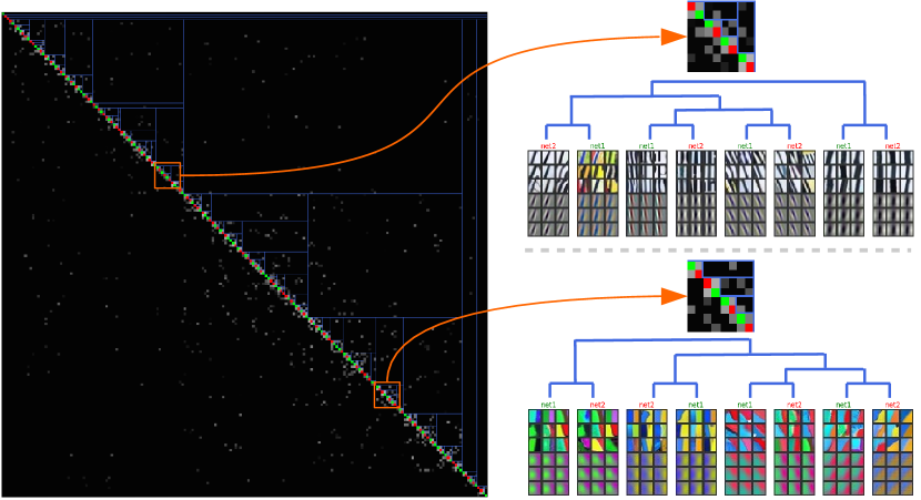
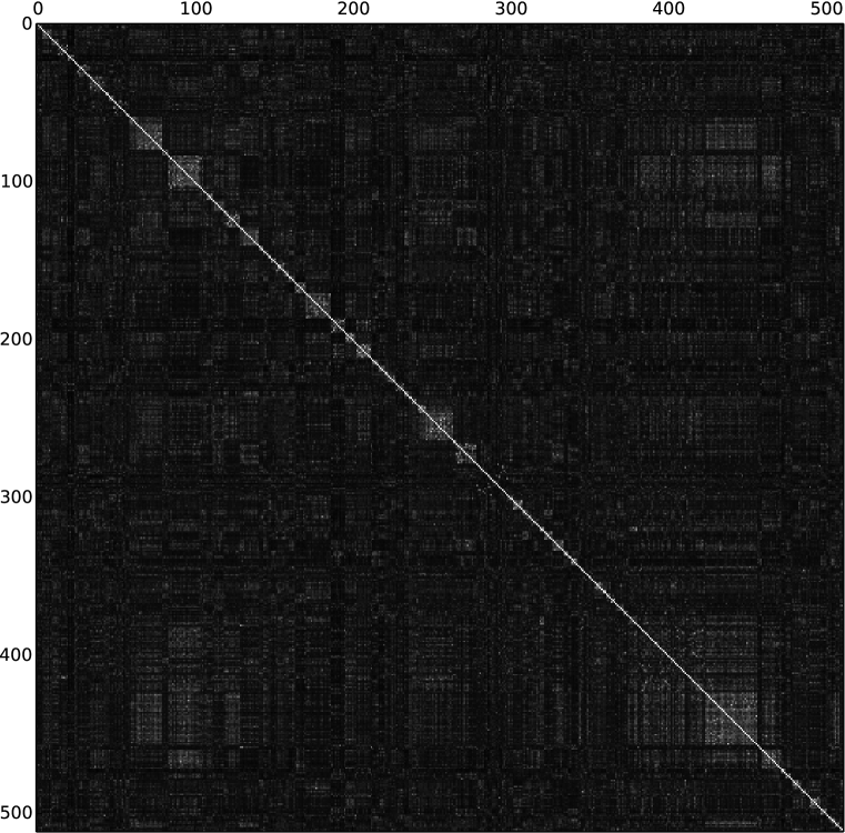
The resulting clustering can be interpreted as a tree with units as leaves, clusters as intermediate nodes, and the single final cluster as the root node. In Figure 7 we plot the matrix with rows and columns permuted together in the order leaves are encountered when traversing the tree, and intermediate nodes are overlaid as lines joining their subordinate units or clusters. For clarity, we color the diagonal pixels (which all have value one) with green or red if the associated unit came from or , respectively.
Plotted in this way, structure is readily visible: Most parents of leaf clusters (the smallest merges shown as two blue lines of length two covering a region) contain one unit from and one from . These units can be considered most predictive of each other.111111Note that the upper right corner of is , the matrix predicting , and the lower left is just the transpose . The corners could instead be and , respectively. Slightly higher level clusters show small subspaces, comprised of multiple units from each network, where multiple units from one network are useful for predicting activations from the other network (see the example zoomed regions on the right side of Figure 7).
The HAC method employs greedy merges, which could in some cases be suboptimal. In the Supplementary Section S.3 we explore a related method that is less greedy, but operates on the denser correlation matrix instead. Future work investigating or developing other methods for analyzing the structure of the sparse prediction matrices may shed further light on the shared, learned subspaces of independently trained networks.

5 Conclusions
We have demonstrated a method for quantifying the feature similarity between different, independently trained deep neural networks. We show how insights may be gain by approximately aligning different neural networks on a feature or subspace level by blending three approaches: a bipartite matching that makes one-to-one assignments between neurons, a sparse prediction and clustering approach that finds one-to-many mappings, and a spectral clustering approach that finds many-to-many mappings. Our main findings include:
-
1.
Some features are learned reliably in multiple networks, yet other features are not consistently learned.
-
2.
Units learn to span low-dimensional subspaces and, while these subspaces are common to multiple networks, the specific basis vectors learned are not.
-
3.
The representation codes are a mix between a local (single unit) code and slightly, but not fully, distributed codes across multiple units.
-
4.
The average activation values of neurons vary considerably within a network, yet the mean activation values across different networks converge to an almost identical distribution.
6 Future Work
The findings in this paper open up new future research directions, for example: (1) Model compression. How would removing low-correlation, rare filters affect performance? (2) Optimizing ensemble formation. The results show some features (and subspaces) are shared between independently trained DNNs, and some are not. This suggests testing how feature correlation among different DNNs in an ensemble affects ensemble performance. For example, the “shared cores” of multiple networks could be deduplicated, but the unique features in the tails of their feature sets could be kept. (3) Similarly, one could (a) post-hoc assemble ensembles with greater diversity, or even (b) directly encourage ensemble feature diversity during training. (4) Certain visualization techniques, e.g., deconv (Zeiler & Fergus, 2014), DeepVis (Yosinski et al., 2015), have revealed neurons with multiple functions (e.g. detectors that fire for wheels and faces). The proposed matching methods could reveal more about why these arise. Are these units consistently learned because they are helpful or are they just noisy, imperfect features found in local optima? (5) Model combination: can multiple models be combined by concatenating their features, deleting those with high overlap, and then fine-tuning? (6) Apply the analysis to networks with different architectures — for example, networks with different numbers of layers or different layer sizes — or networks trained on different subsets of the training data. (7) Study the correlations of features in the same network, but across training iterations, which could show whether some features are trained early and not changed much later, versus perhaps others being changed in the later stages of fine-tuning. This could lead to complementary insights on learning dynamics to those reported by Erhan et al. (2009). (8) Study whether particular regularization or optimization strategies (e.g., dropout, ordered dropout, path SGD, etc.) increase or decrease the convergent properties of the representations to facilitate different goals (more convergent would be better for data-parallel training, and less convergent would be better for ensemble formation and compilation).
Acknowledgments
The authors are grateful to the NASA Space Technology Research Fellowship (JY) for funding, Wendy Shang for conversations and initial ideas, Yoshua Bengio for modeling suggestions, and Anh Nguyen and Kilian Weinberger for helpful comments and edits. This work was supported in part by US Army Research Office W911NF-14-1-0477, NSF grant 1527232. Jeff Clune was supported by an NSF CAREER award (CAREER: 1453549) and a hardware donation from the NVIDIA Corporation.
References
- Arora et al. (2014) Arora, Sanjeev, Bhaskara, Aditya, Ge, Rong, and Ma, Tengyu. Provable bounds for learning some deep representations. In ICML, pp. 584–592, 2014.
- Dauphin et al. (2014) Dauphin, Yann, Pascanu, Razvan, Gülçehre, Çaglar, Cho, Kyunghyun, Ganguli, Surya, and Bengio, Yoshua. Identifying and attacking the saddle point problem in high-dimensional non-convex optimization. CoRR, abs/1406.2572, 2014. URL http://arxiv.org/abs/1406.2572.
- Deng et al. (2009) Deng, Jia, Dong, Wei, Socher, Richard, Li, Li-Jia, Li, Kai, and Fei-Fei, Li. Imagenet: A large-scale hierarchical image database. In Computer Vision and Pattern Recognition, 2009. CVPR 2009. IEEE Conference on, pp. 248–255. IEEE, 2009.
- Eigen et al. (2013) Eigen, David, Rolfe, Jason, Fergus, Rob, and LeCun, Yann. Understanding deep architectures using a recursive convolutional network. arXiv preprint arXiv:1312.1847, 2013.
- Erhan et al. (2009) Erhan, Dumitru, Manzagol, Pierre-Antoine, Bengio, Yoshua, Bengio, Samy, and Vincent, Pascal. The difficulty of training deep architectures and the effect of unsupervised pre-training. In International Conference on artificial intelligence and statistics, pp. 153–160, 2009.
- Goodfellow et al. (2014) Goodfellow, Ian J, Shlens, Jonathon, and Szegedy, Christian. Explaining and Harnessing Adversarial Examples. ArXiv e-prints, December 2014.
- Hopcroft & Karp (1973) Hopcroft, John E and Karp, Richard M. An n^5/2 algorithm for maximum matchings in bipartite graphs. SIAM Journal on computing, 2(4):225–231, 1973.
- Jia et al. (2014) Jia, Yangqing, Shelhamer, Evan, Donahue, Jeff, Karayev, Sergey, Long, Jonathan, Girshick, Ross, Guadarrama, Sergio, and Darrell, Trevor. Caffe: Convolutional architecture for fast feature embedding. arXiv preprint arXiv:1408.5093, 2014.
- Krizhevsky et al. (2012) Krizhevsky, Alex, Sutskever, Ilya, and Hinton, Geoff. Imagenet classification with deep convolutional neural networks. In Advances in Neural Information Processing Systems 25, pp. 1106–1114, 2012.
- Lawler (1976) Lawler, Eugene L. Combinatorial optimization: networks and matroids. Courier Corporation, 1976.
- Lenc & Vedaldi (2015) Lenc, Karel and Vedaldi, Andrea. Understanding image representations by measuring their equivariance and equivalence. The IEEE Conference on Computer Vision and Pattern Recognition (CVPR), 2015.
- Mahendran & Vedaldi (2014) Mahendran, Aravindh and Vedaldi, Andrea. Understanding deep image representations by inverting them. arXiv preprint arXiv:1412.0035, 2014.
- Montavon et al. (2011) Montavon, Grégoire, Braun, Mikio L, and Müller, Klaus-Robert. Kernel analysis of deep networks. The Journal of Machine Learning Research, 12:2563–2581, 2011.
- Neyshabur & Panigrahy (2013) Neyshabur, Behnam and Panigrahy, Rina. Sparse matrix factorization. arXiv preprint arXiv:1311.3315, 2013.
- Nguyen et al. (2014) Nguyen, Anh, Yosinski, Jason, and Clune, Jeff. Deep neural networks are easily fooled: High confidence predictions for unrecognizable images. arXiv preprint arXiv:1412.1897, 2014.
- Paul & Venkatasubramanian (2014) Paul, Arnab and Venkatasubramanian, Suresh. Why does deep learning work?-a perspective from group theory. arXiv preprint arXiv:1412.6621, 2014.
- Pedregosa et al. (2011) Pedregosa, F., Varoquaux, G., Gramfort, A., Michel, V., Thirion, B., Grisel, O., Blondel, M., Prettenhofer, P., Weiss, R., Dubourg, V., Vanderplas, J., Passos, A., Cournapeau, D., Brucher, M., Perrot, M., and Duchesnay, E. Scikit-learn: Machine learning in Python. Journal of Machine Learning Research, 12:2825–2830, 2011.
- Simonyan et al. (2013) Simonyan, Karen, Vedaldi, Andrea, and Zisserman, Andrew. Deep inside convolutional networks: Visualising image classification models and saliency maps. arXiv preprint arXiv:1312.6034, presented at ICLR Workshop 2014, 2013.
- Szegedy et al. (2013) Szegedy, Christian, Zaremba, Wojciech, Sutskever, Ilya, Bruna, Joan, Erhan, Dumitru, Goodfellow, Ian J., and Fergus, Rob. Intriguing properties of neural networks. CoRR, abs/1312.6199, 2013.
- Tibshirani (1996) Tibshirani, Robert. Regression shrinkage and selection via the lasso. Journal of the Royal Statistical Society. Series B (Methodological), pp. 267–288, 1996.
- Yosinski et al. (2014) Yosinski, J., Clune, J., Bengio, Y., and Lipson, H. How transferable are features in deep neural networks? In Ghahramani, Z., Welling, M., Cortes, C., Lawrence, N.D., and Weinberger, K.Q. (eds.), Advances in Neural Information Processing Systems 27, pp. 3320–3328. Curran Associates, Inc., December 2014.
- Yosinski et al. (2015) Yosinski, Jason, Clune, Jeff, Nguyen, Anh, Fuchs, Thomas, and Lipson, Hod. Understanding neural networks through deep visualization. In Deep Learning Workshop, International Conference on Machine Learning (ICML), 2015.
- Zeiler & Fergus (2014) Zeiler, Matthew D and Fergus, Rob. Visualizing and understanding convolutional networks. In ECCV, pp. 818–833, 2014.
- Zhou et al. (2014) Zhou, Bolei, Khosla, Aditya, Lapedriza, Àgata, Oliva, Aude, and Torralba, Antonio. Object detectors emerge in deep scene cnns. In International Conference on Learning Representations (ICLR), volume abs/1412.6856, 2014. URL http://arxiv.org/abs/1412.6856.
Supplementary Information
Appendix S.1 Activation Values: High Correlation vs. Low Correlation


Appendix S.2 Additional Matching Results
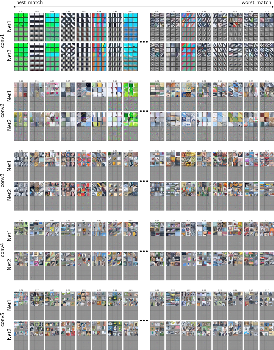
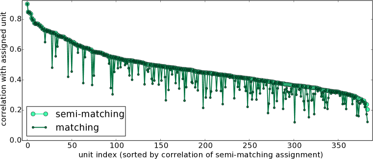
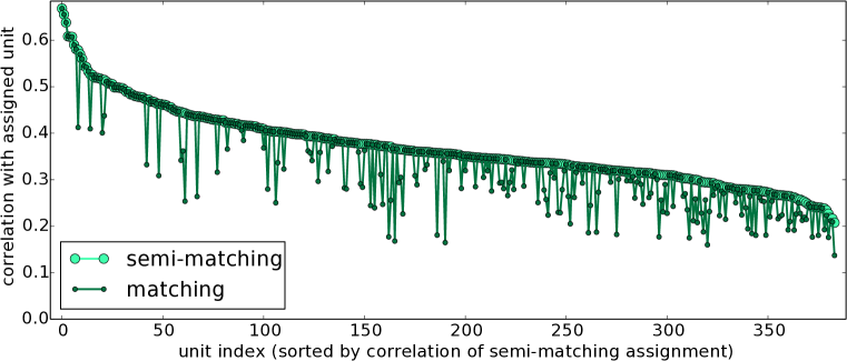
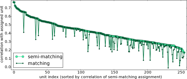
Figure S3 shows additional results of comparison of assignments produced by semi-matching and matching methods in – . For each unit, both the semi-matching and matching are found, then the units are sorted in order of decreasing semi-matching value and both correlation values are plotted.

Appendix S.3 Does Relaxing the One-to-One Constraint to Find Many-to-Many Groupings Reveal More Similarities Between what Different Networks Learn?
Since the preceding sections have shown that neurons may not necessarily correspond via a globally consistent one-to-one matching between networks, we now seek to find many-to-many matchings between networks using a spectral clustering approach.
S.3.1 Neuron Similarity Graphs
We define three types of similarity graphs based on the correlation matrices obtained above.
Single-net neuron similarity graphs. Given a fully trained DNN and a specified layer , we first construct the single-net neuron similarity graph . Each vertex in this graph represents a unit in layer . Two vertices are connected by an edge of weight if the correlation value in the self-correlation matrix between unit and unit is greater than a certain threshold .
Between-net neuron similarity graphs. Given a pair of fully trained DNNs and , the between-net neuron similarity graph can be constructed in a similar manner. Note that is a bipartite graph and contains twice as many vertices as that in since it incorporates units from both networks. Two vertices are connected by an edge of weight if the correlation value in the between-net correlation matrix between unit in and unit in is greater than a certain threshold .
Combined similarity graphs. The problem of matching neurons in different networks can now be reformulated as finding a partition in the combined neuron similarity graphs , such that the edges between different groups have very low weights and the edges within a group have relatively high weights.
S.3.2 Spectral Clustering and Metrics for Neuron Clusters
We define three types of similarity graphs based on the correlation matrices obtained above (see Section S.3.1 for definition). Define to be the combined correlation matrices between two DNNs, and in layer , where is the entry at th row and th column of that matrix. is the number of channels (units) in layer . is given by
The unnormalized Laplacian matrix is defined as , where the degree matrix is the diagonal matrix with the degrees . The unnormalized Laplacian matrix and its eigenvalues and eigenvectors can be used to effectively embed points in a lower-dimension representation without losing too information about spatial relationships. If neuron clusters can be identified, then the Laplacian is approximately block-diagonal, with each block corresponding a cluster. Assuming there are clusters in the graph, spectral clustering would then take the first eigenvectors121212In practice, when the number of clusters is unknown, the best value of to choose is where where the eigenvalue shows a relatively abrupt change., , corresponding to the smallest eigenvalues, and partition neurons in the eigenspace with the -means algorithm.
S.3.3 Spectral Clustering Results
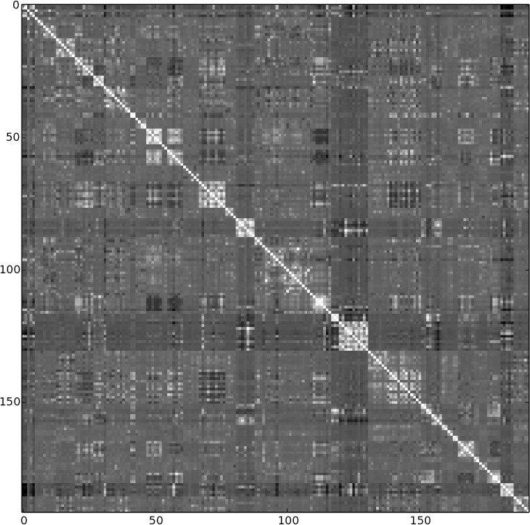
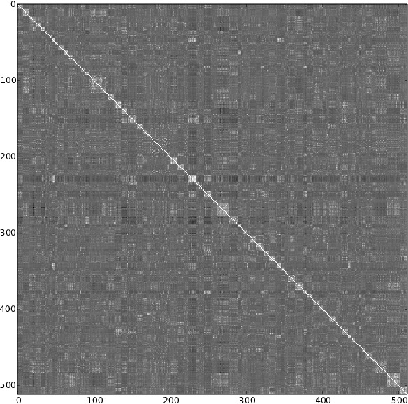
We use and as an example for showing the results of matching neurons between DNNs. Figure S5 shows the permuted combined correlation matrix after apply the spectral clustering algorithm for – . Figure S6 displays 12 neuron clusters with high between-net similarity measurement in layer, and Figure S7 displays the top 8 neuron clusters with highest between-net similarity measurement in layer. The matching results imply that there exists many-to-many correspondence of the feature maps between two fully trained networks with different random initializations, and the number of neurons learning the same feature can be different between networks. For example, the four units of {89, 90, 134, 226} in and three units of {2, 39, 83} in are learning the features about green objects.
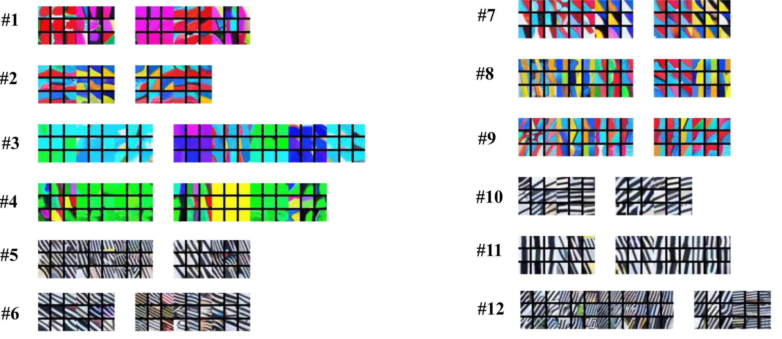

We also computed and visualized the matching neurons in other layers as well. The results of are shown in Figure S6. As noted earlier, the layer tends to learn more general features like Gabor filters (edge detectors) and blobs of color. Our approach finds many matching Gabor filters (e.g., clusters #5, #6, #10, #11 and #12), and also some matching color blobs (e.g., clusters #1, #3 and #4).
S.3.4 Hierarchical Spectral Clustering Results
Due to the stochastic effects of randomly initializing centroids in -means clustering, some of the initial clusters contains more neurons than others. To get more fine-grained cluster structure, we recurrently apply -means clustering on any clusters with size , where is a tunable parameter for adjusting the maximum size of the leaf clusters. Figure S8 shows the partial hierarchical structure of neuron matchings in the layer. The cluster at the root of the tree is a first-level cluster that contains many similar units from both DNNs. Here we adopt for the layer, resulting in a hierarchical neuron cluster tree structure with leaf clusters containing less than 6 neurons from each network. The bold box of each subcluster contains neurons from and the remaining neurons are from . For example, in subcluster #3, which shows features, units {62, 137, 148} from learned similar features as units {33, 64, 230} from , namely, red and magenta objects.

S.3.5 Metrics for Neuron Clusters
Here we introduce two metrics for quantifying the similarity among neurons grouped together after applying the clustering algorithm above.
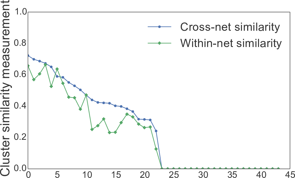
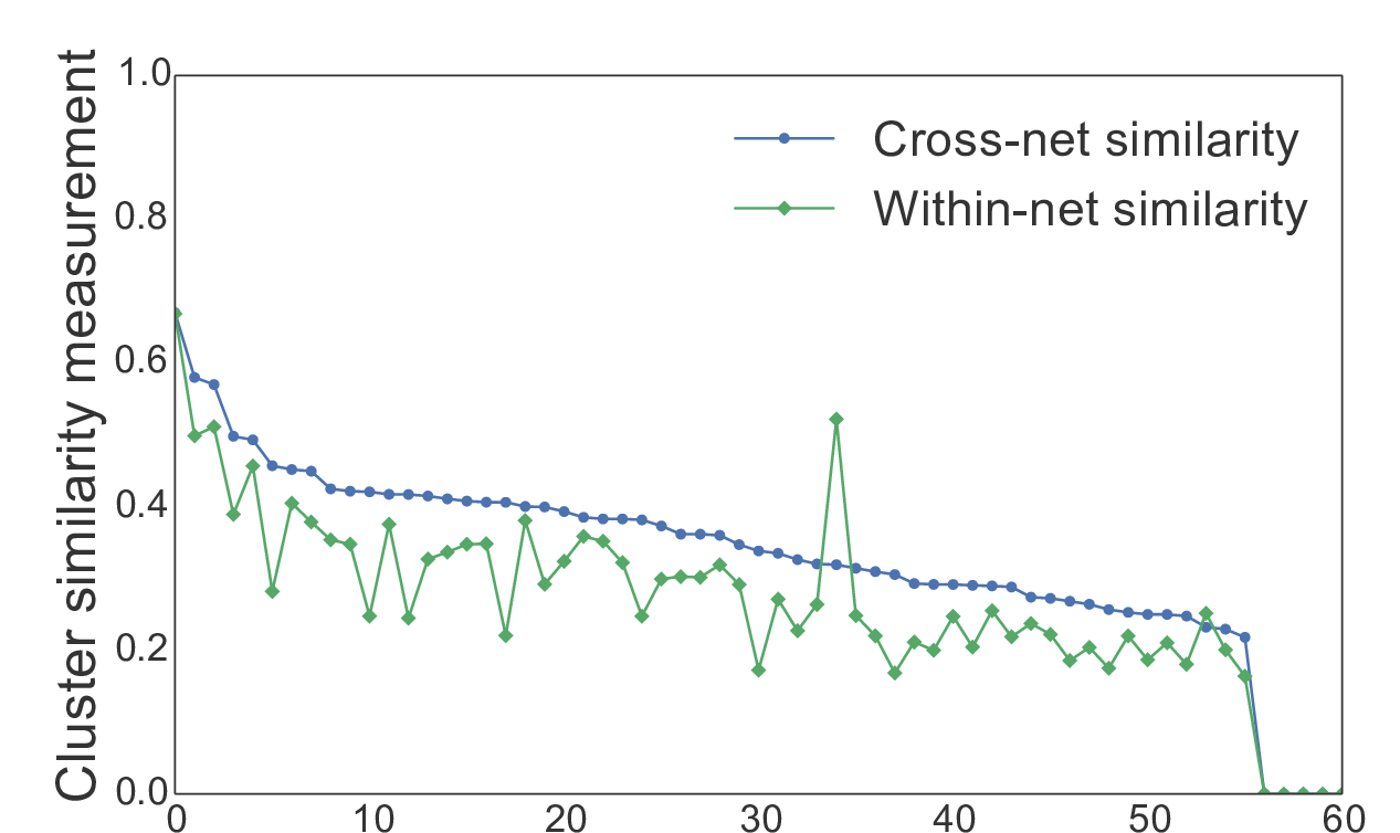
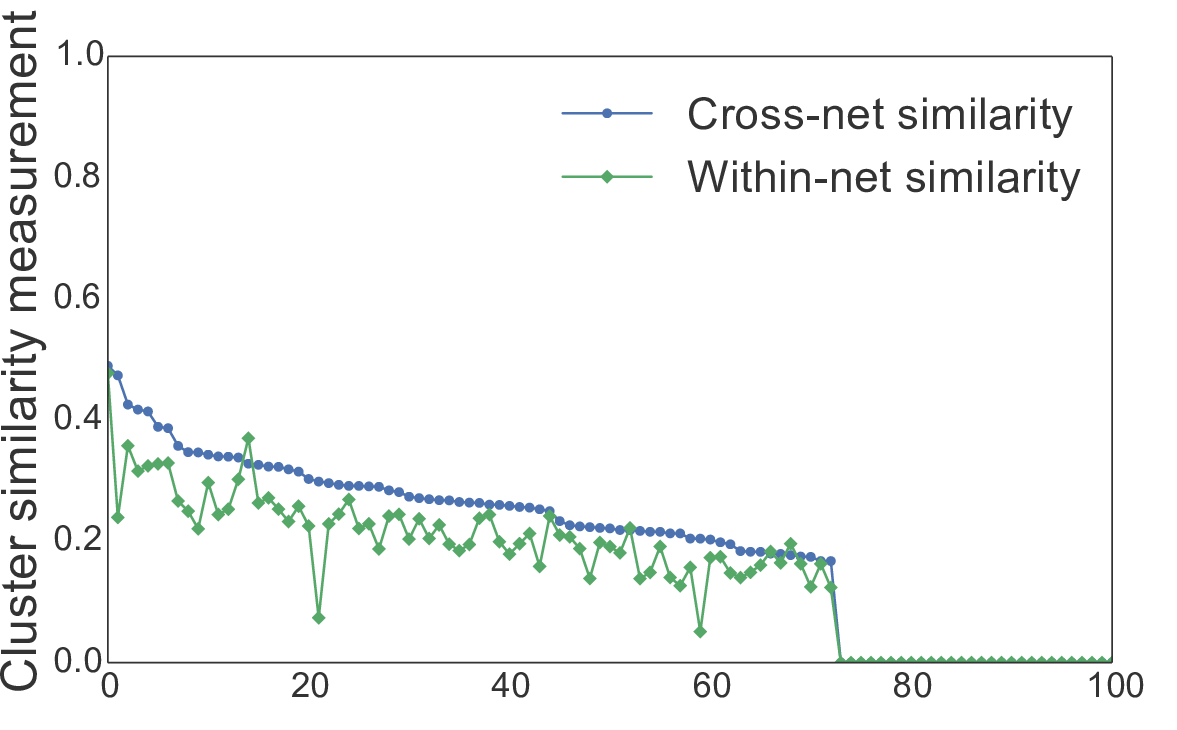
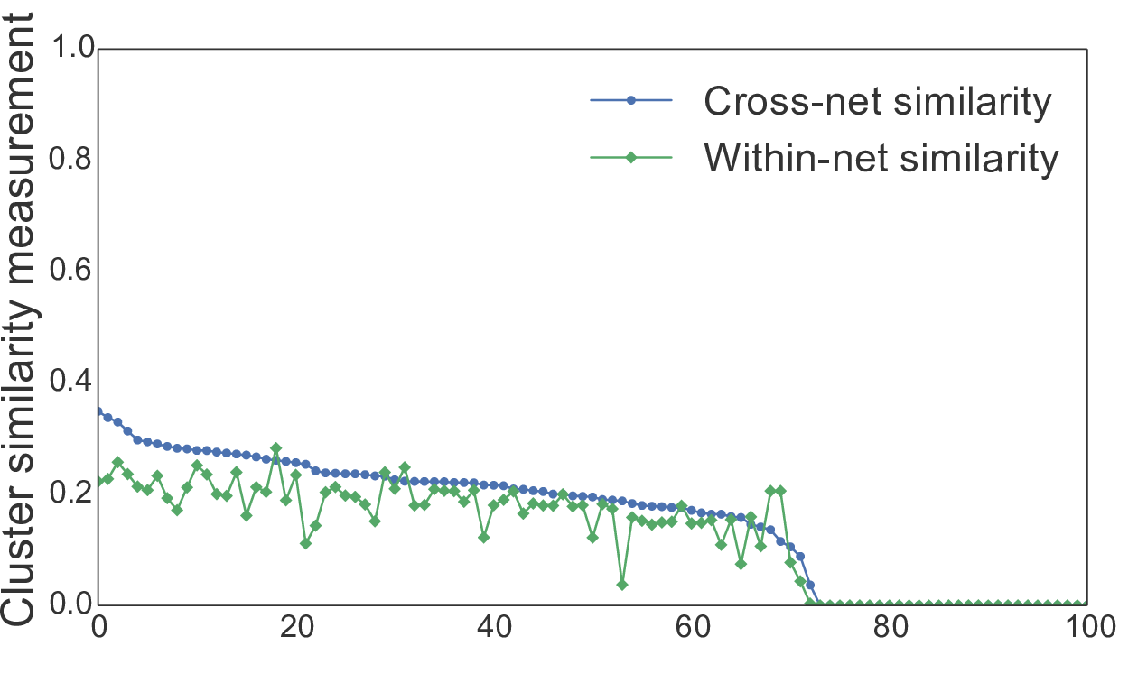
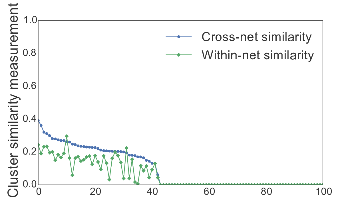
We further performed experiments in quantifying the similarity among neurons that are clustered together. Figure S9 shows the between-net and within-net similarity measurement for – . The value of for initial clustering is set to be 40 for layer and 100 for all the other layers. In our experiments, the number of final clusters obtained after further hierarchical branching is {43, 113, 130, 155, 131}. The tail in those curves with value 0 is due to the non-existence of between-net similarity for the clusters containing neurons from only one of the two DNNs. To better capture the distribution of non-zero similarity values, we leave out the tail after 100 in the plot for - layers.
Appendix S.4 Comparing Average Neural Activations within and between Networks
The first layer of networks trained on natural images (here the layer) tends to learn channels matching patterns similar to Gabor filters (oriented edge filters) and blobs of color. As shown in Figures S10, S11, and S12, there are certain systematic biases in the relative magnitudes of the activations of the different channels of the first layer. Responses of the low frequency filters have much higher magnitude than that of the high frequency filters. This phenomenon is likely a consequence of the power spectrum of natural images in which, on average, low spatial frequencies tend to contain higher energy (because they are more common) than high spatial frequencies.

In Figure S10 we show the mean activations for each unit of four networks, plotted in sorted order from highest to lowest. First and most saliently, we see a pattern of widely varying mean activation values across units, with a gap between the most active and least active units of one or two orders of magnitude (depending on the layer). Second, we observe a rough overall correspondence in the spectrum of activations between the networks. However, the correspondence is not perfect: although much of the spectrum matches well, the most active filters converged to solutions of somewhat different magnitudes. For example, the average activation value of the filter on with the highest average activation varies between 49 to 120 over the four networks; the range for was 98 to 130.131313Recall that the units use rectified linear activation functions, so the activation magnitude is unbounded. The max activation over all channels and all spatial positions of the first layer is often over 2000. This effect is more interesting considering that all filters were learned with constant weight decay, which pushes all individual filter weights and biases (and thus subsequent activations) toward zero with the same force.
Figure S11 shows the units with the highest and lowest activations for each of the four networks. As mentioned earlier (and as expected), filters for lower spatial frequencies have higher average activation, and vice versa. What is surprising is the relative lack of ordering between the four networks. For example, the top two most active filters in respond to constant color regions of black or light blue, whereas none of the top eight filters in or respond to such patterns. One might have thought that whatever influence from the dataset caused the largest filters to be black and blue in the first network would have caused similar constant color patches to dominate the other networks, but we did not observe such consistency. Similar differences exist when observing the learned edge filters: in and the most active edge filter is horizontal; in and it is vertical. The right half of Figure S11 depicts the least active filters. The same lack of alignment arises, but here the activation values are more tightly packed, so the exact ordering is less meaningful. Figure S12 shows the even more widely varying activations from .

