Learning Visual Predictive Models of Physics for Playing Billiards
Abstract
The ability to plan and execute goal specific actions in varied and unseen environments settings is a central requirement of intelligent agents. In this paper, we explore how an agent can be equipped with an internal model of the dynamics of the external world, and how it can use this model to plan novel actions by running multiple internal simulations (“visual imagination”). Our models directly process raw visual input, and use a novel object-centric prediction formulation based on visual glimpses centered on objects (fixations) to enforce translational invariance of the learned physical laws. The agent trains itself through random interaction with a collection of different environments, and the resulting model can then be used to plan goal-directed actions in novel environments that were previously never encountered by the agent. We demonstrate that our agent can accurately plan actions for playing a simulated billiards game, which requires pushing a ball into a target position or into collision with another ball.
1 Introduction
Imagine a hypothetical person who has never encountered the game of billiards. While this person may not be very adept at playing the game, he would still be capable of inferring the direction in which the cue ball needs to be hit to displace the target ball to a desired location. How can this person make such an inference without any prior billiards-specific experience? One explanation is that humans are aware of the laws of physics, and a strategy for playing billiards can be inferred from knowledge about dynamics of bouncing objects. However, humans do not appear to consciously solve Newton’s equations of motion, but rather have an intuitive understanding of how their actions affect the world. In the specific example of billiards, humans can imagine the trajectory that the ball would follow when a force is applied, and how the trajectory of ball would change when it hits the side of the billiards table or another ball. We term models that can enable the agents to visually anticipate the future states of the world as visual predictive models of physics.
A visual predictive model of physics equips an agent with the ability to generate potential future states of the world in response to an action without actually performing that action (“visual imagination”). Such visual imagination can be thought of as running an internal simulation of the external world. By running multiple internal simulations to imagine the effects of different actions, the agent can perform planning, choosing the action with the best outcome and executing it in the real world. The idea of using internal models for planning actions is well known in the control literature (Mayne, 2014). However, the question of how such models can be learned from raw visual input has received comparatively little attention, particularly in situations where the external world can change significantly, requiring generalization to a variety of environments and situations.
Previous methods have addressed the question of learning models, including visual models, of the agent’s own body (Watter et al., 2015; Lillicrap et al., 2015). However, when performing actions in complex environments, models of both the agent and the external world are required. The external world can exhibit considerably more variation than the agent itself, and therefore such models must generalize more broadly. This makes problem of modelling the environment substantially harder than modelling the agent itself.
The complexities associated with modeling the external world may be elucidated through an example. Consider the family of worlds composed of moving balls on a 2D table (i.e. moving-ball world). This family contains diverse worlds that can be generated by varying factors such as the number of balls, the table geometries, ball sizes, the colors of balls and walls, and the forces applied to push the balls. Because the number of objects can change across worlds, it is not possible to explicitly define a single state space for these worlds. For the purpose of modeling, an implicit state space must be learnt directly from visual inputs. In addition to this combinatorial structure, differences in geometry and nonlinear phenomena such as collisions result in considerable complexity.
Similar to the real world, in the moving-ball world, an agent must perform actions in novel conditions it has never encountered before. Although moving-ball worlds are relatively constrained and synthetic, the diversity of such worlds can be manipulated using a small number of factors. This makes them a good case study for systematically evaluating and comparing the performance of different model-based action selection methods under variation in external conditions (i.e. generalization).
Both the real world and the synthetic moving-ball worlds also contain regularities that allow learning generalizable models in the face of extensive variation, such as the translational invariance of physical laws. The main contribution of this work is a first step towards learning dynamical model of the external world directly from visual inputs that can handle combinatorial structure and exploits translation invariance in dynamics. We propose an object-centric (OC) prediction approach, illustrated in Figure 1), that predicts the future states of the world by individually modeling the temporal evolution of each object from object-centric glimpses. The object-centric (OC) approach naturally incorporates translation invariance and model sharing across different worlds and object instances.

We use a simulated billiards-playing domain where the agent can push balls on a 2D billiard table with varying geometry as a working example to evaluate our approach. We show that our agent learns a model of the billiards world that can be used to effectively simulate the movements of balls and consequently plan actions without requiring any goal-specific supervision. Our agent successfully predicts forces required to displace the ball to a desired location on the billiards table and to hit another moving ball.
2 Previous Work
Vision-based control
Due to the recent success of deep neural networks for learning feature representations that can handle the complexity of visual input Krizhevsky et al. (2012), there has been considerable interest in utilizing this capability for learning to control dynamical systems directly from visual input. Methods that directly learn policies for prediction actions from visual inputs have been successfully used to learn to play Atari games Mnih et al. (2013) and control a real robot for a predefined set of manipulation tasks Levine et al. (2015). However, these methods do not attempt to model how visual observations will evolve in response to agent’s actions. This makes it difficult to repurpose the learned policies for new tasks.
Another body of work (Kietzmann & Riedmiller, 2009; Lange et al., 2012) has attempted to build models that transform raw sensory observations into a low-dimensional feature space that is better suited for reinforcement learning and control. More recently works such as (Wahlström et al., 2015; Watter et al., 2015) have shown successful results on relatively simple domains of manipulating a synthetic two degree of freedom robotic arm or controlling an inverted pendulum in simulation. However, training and testing environments in these works were exactly the same. In contrast, our work shows that vision based model predictive control can be used in scenarios where the test environments are substantially different from training environments.
Models of physics and model based control
(Hamrick et al., 2011) provided evidence that human judgement of how dynamical systems evolve in future can be explained by the hypothesis that humans use internal models of physics. (Jordan & Rumelhart, 1992; Wolpert et al., 1995; Haruno et al., 2001; Todorov & Ghahramani, 2003) proposed using internal models of the external world for planning actions. However these works have either been theoretical or have striven to explain sensorimotor learning in humans. To the best of our knowledge we are the first work that strives to build an internal model of the external world purely from visual data and use it for planning novel actions. (Oh et al., 2015) successfully predict future frames in Atari game videos and train a Q-controller for playing Atari games using the predicted frames. Training a Q-controller requires task specific supervision whereas our work explores whether effective dynamical models for action planning can be learnt without requiring any task specific supervision.
Learning Physics from Images and Videos
Works of Wu et al. (2015); Bhat et al. (2002); Brubaker et al. (2009); Mottaghi et al. (2015) propose methods for estimating the parameters of Newtonian equations from images and videos. As laws of physics governing the dynamics of balls and walls on a billiards table are well understood, it is possible to use these laws instead of learning a predictive model for planning actions. However, there are different dynamic models that control ball-ball collisions, ball-wall collisions and the movement of ball in free space. Therefore, if these known dynamical model are to be used, then a system for detecting different event types would be required for selecting the appropriate dynamics model at different time points. In contrast, our approach avoids hand designing such event detectors and switches and provides a more general and scalable solution even in the case of billiards.
Video prediction
(Michalski et al., 2014; Sutskever et al., 2008) learn models capable of generating images of bouncing balls. However, these models are not shown to generalize to novel environments. Further these works donot include any notion of an agent or its influence on the environment. (Boots et al., 2014) proposes model for predicting the future visual appearance of a robotic arm, but the method is only shown to work when the same object in the same visual environment is considered. Further it is not obvious how the non-parametric approach would scale with large datasets. In contrast our approach generalized to novel environments and can scale easily with large amounts of data.
Motion prediction for Visual Tracking
In Computer Vision, object trackers use a wide variety of predictive models, from simple constant velocity models, to linear dynamical systems and their variants (Urtasun et al., 2006), HMMs (Brand et al., 1997; Ghahramani & Jordan, 1997), and other models. Standard smoothers or filters, such as Kalman filters (Weng et al., 2006), usually operate on Cartesian coordinates, rather than the visual content of the targets, and in this way discard useful information that may be present in the images. Finally, methods for 3D tracking of Kyriazis et al. (2011); Salzmann & Urtasun (2011) use Physics simulators to constrain the search space during data association.
3 Learning Predictive Visual Models
We consider an agent observing an interacting with dynamic moving-ball worlds consisting of multiple balls and multiple walls. We also refer to these worlds as billiard worlds. The agent interacts with the world by applying forces to change the velocities of the balls. In the real world, the environment of an agent is not fixed, and the agent can find itself in environments that it has not seen before. To explore this kind of generalization, we train our predictive model in a variety of billiards environments, which involve different numbers of balls and different wall geometries, and then test the learnt model in previously unseen settings.
In the case of moving-ball world, it is sufficient to predict the displacement of the ball during the next time step to generate the visual of the world in the future. Therefore, instead of directly predicting image pixels, we predict each object’s current and future velocity given a sequence of visual glimpses centered at the object (visual fixation) and the forces applied to it.
We assume that during training the agent can perfectly track the objects. This assumption is a mild one because not only tracking is a well studied problem but also because there is evidence in the child development literature that very young infants can redirect their gaze to keep an object in focus by anticipating its motion (i.e. smooth pursuit) (Hofsten & Rosander, 1997). The early development of smooth pursuit suggests that it is important for further development of visual and motor faculties of a human infant.
3.1 Model Details
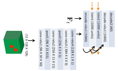
Our network architecture is illustrated in figure 2. The input to the model is a stack of 4 images comprised of the current and previous 3 glimpses of the fixated object and the exercised force on the object at the current time step. The model predicts the velocity of the object at each of the time steps in the future. We use = 20. The same model is applied to all the objects in the world.
Our network uses an AlexNet style architecture (Krizhevsky et al., 2012) to extract visual features. The first layer (conv1) is adapted to process a stack of 4 frames. Layers 2 and 3 have the same architecture as that of AlexNet. Layer 4 (conv4) is composed of 128 convolution kernels of size . The output of conv4 is rescaled to match the value range of the applied forces, then is concatenated with the current force and is passed into a fully connected (encoder) layer. Two layers of LSTM units operate on the output of the encoder to model long range temporal dynamics. Then, the output is decoded to predicted velocities.
The model is trained by minimizing the Euclidean loss between ground-truth and predicted object velocities for time steps in the future. The ground-truth velocities are known because we assume object tracking. The loss is mathematically expressed as:
| (1) |
where represent ground-truth and predicted velocities at the time step in the future respectively. Velocities are expressed in cartesian coordinates. We weigh the loss in a manner that errors in predictions at a shorter time horizon are penalized more than predictions at a longer time horizon. This weighting is achieved using penalty weights . We use the publicly available Caffe package for training our model.
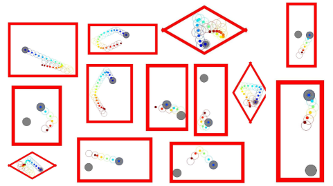
For model learning, we generate sequences of ball motions in a randomly sampled world configuration. As shown in Figure 3, we experimented both with rectangular and non-rectangular wall geometries. For rectangular walls, a single sample of the world was generated by randomly choosing the size of the walls, location of the balls and the forces applied on the balls from a predefined range. The length of each sequence was sampled from the range [20, 200]. The length of the walls was sampled from a range of [300 pixels, 550 pixels]. Balls were of radius 25 pixels and uniform density. Force direction was uniformly sampled and the force magnitude was sampled from the range [30K Newtons, 80K Newtons]. Forces were only applied on the first frame. The size of visual glimpses is 600x600 pixels. The objects can move up to 10 pixels in each time step and therefore in 20 time steps they can cover distances up to 200 pixels.
For training, we pre-generated 10K such sequences. We constructed minibatches by choosing 50 random subsets of 20 consequent frames from this pre-generated dataset. Weights in layers conv2 and conv3 were initialized from the weights of Alexnet that was trained for performing image classification on Imagenet (Krizhevsky et al., 2012). Weights in other layers are randomly initialized.
4 Model Evaluation
First we report evaluations on random worlds sampled from the same distribution as the training data. Next, we report evaluations on worlds sampled from a different distribution of world configurations to study the generalization of the proposed approach. Error in the angle and magnitude of the predicted velocities were used as performance metrics. We compared the performance of the proposed object centric (OC) model with a constant velocity (CV) and frame centric (FC) model. The constant velocity model predicts the velocity of a ball for all the future frames to be same as the ground truth velocity at the previous time step. The ball changes the velocity only when it strikes another ball or hits a wall. As collisions are relatively infrequent, the constant velocity model is a good baseline.
We first trained a model on the family of rectangular worlds consisting of 1 ball only. The results of this evaluation are reported in Table 1. We used average error across all the frames and the error averaged across frames only near the collisions as the error metrics for measuring performance. As balls move in linear trajectories except for time of collision, accurately predicting the velocities after a collision event is of specific interest. Results in Table 1 show that the object centric (OC) model is better than frame centric model (FC) model and much better than the constant velocity model. These results show that object centric modelling leads to better learning.
| Time | Overall Error | Error Near Collisions | ||||
|---|---|---|---|---|---|---|
| CV | FC | OC | CV | FC | OC | |
| t+1 | /0.00 | /0.04 | /0.00 | /0.06 | /0.04 | |
| t+5 | /0.01 | /0.05 | /0.05 | /0.12 | /0.10 | |
| t+20 | /0.01 | /0.09 | /0.04 | /0.20 | /0.20 | |
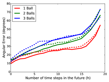
How well does our model scale with increasing number of balls? For studying this, we trained models on families of world consisting of 2 and 3 balls respectively. We used the learnt 1-ball model to initialize the training of the 2-ball model, which in turn was used to initialize the training of the 3-ball model. We found this curriculum learning approach to outperform models trained from scratch. The 2 and 3-ball models were evaluated on worlds separate from training set that consisted of 2 and 3 ball respectively. The angular errors measured near collisions (for 1 to 20) are shown Figure 4. The performance of our model degrades only by small amounts as the number of balls increase. Also, in general the OC model performs better than the FC model.
We also trained and tested our models on non-rectangular walls. Qualitative visualizations of ground truth and predicted ball trajectories are show in figure 3. The figure shows that our model accurately predicts the velocities of balls after collisions in varied environments. This result indicates that our models are not constrained to any specific environment and have learnt something about the dynamics of balls and their collisions.
4.1 Evaluating Generalization
The results reported in the previous section show generalization to worlds sampled from the same distribution as the training set. In addition to this, we also tested our models on worlds substantially different from the worlds in the training set.
Figure 7 shows that our model can generalize to much larger wall configurations than those used in the training. The wall lengths in the training set were between 300-550 pixels, whereas the the wall lengths in the testing set were sampled from the range of 800-1200 pixels. This shows that our models can generalize to different wall geometries.
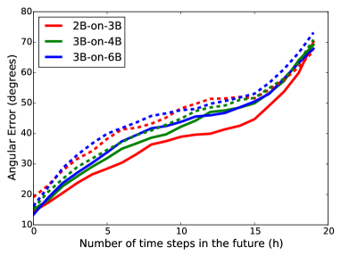
Figure 4 (right) shows that models trained on 2 and 3-ball worlds perform well when tested on 3, 4 and 6-ball worlds. This shows that our models can generalize to worlds with larger number of balls without requiring any additional training. The results in the figure also show that proposed OC model generalizes substantially better than the FC model.
5 Generating Visual Imaginations
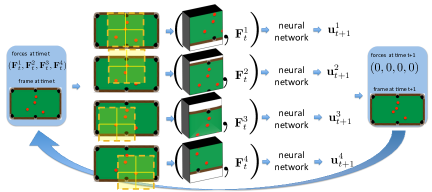
As our models can accurately predict ball dynamics in the future, we can use these models to generate visual imaginations of the future. The procedure we use for generating visual imaginations is illustrated in figure 5. Given a configuration of the world and applied forces, the visual image of the world at the time step is generated by translating each ball by amount to equal to its predicted velocity () at time . This generated image forms the input to the model for generating the visual image of the world at time step . This process is repeated iteratively to generate visual imaginations of the future world states.
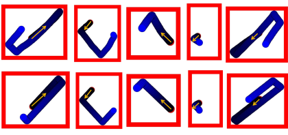
Some examples of visual imaginations by our model are shown in figure 6. Our model learns to anticipate collisions early in time. Predicting trajectory reversals at collisions is not possible using methods Kalman filter based methods that are extensively used in object tracking(Welch & Bishop, 1995). Comparison with ground truth trajectories reveals that our models are not perfect and in some cases accumulation of errors can produce imagined trajectories that are different from the ground truth trajectories (for instance see the first column in figure 6). Even in the cases when predicted trajectories do not exactly match up with the ground truth trajectories, the visual imaginations are consistent with the dynamics of balls and collisions.
Figure 7 shows visual imaginations by our model in environments that are much larger than the environments used in the training set. Notice that the glimpse size is considerably smaller than the size of the environment. With glimpses of this size, visual inputs when the ball is not close to any of the walls are uninformative because such visual inputs merely comprise of a ball present in center of white background. In such scenarios, our model is able to make accurate predictions of velocity due to the long-range LSTM memory of the past. Without LSTM units, we noticed that imagined ball trajectory exhibited unexpected reversal in directions and other errors. For more examples, please see accompanying video for imaginations in two and three ball worlds.

6 Using Predictive Visual Models for Action Planning
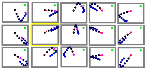
We used the learnt predictive models for planning actions to achieve goals which the agent has never received any direct supervision. We first show results on a relatively simple task of planning the force required to push the desired ball to a desired location. Next, we show results on a more challenging task of planning the force required to push the desired ball to hit a second moving ball.
Figure 8 illustrates the method of action planning. Given a target state, the optimal force is found by running multiple simulations (i.e. visual imaginations) of the world after applying different forces. The optimal force is the one that produces the world state that is closest to the target state. In order to verify the accuracy of this method, we use the predicted force from our model as input to our physics engine to generate its actual (rather than the imagined) outcome and compare the resulting states against the goal states. In practice, instead of exhaustively searching for all forces we use CMA-ES method (Hansen & Ostermeier, 2001) for determining the optimal force.
Table 2 reports the hit accuracy of our system in pushing the ball to a desired location. The hit accuracy was measured as the number of trials for which the closest point on the ball’s trajectory was within pixels of the target. With an accuracy of 56% our model is able to push the ball within 25 pixels (the size of the arena was between 300-550 pixels in size) of the target location as compared to the oracle which is successful 100% times. The OC model significantly outperforms the FC model. The oracle was constructed by using the ground truth physics simulator for making predictions and used the same mechanism for action selection as described above. Qualitative results of our methods are best seen in the accompanying video. We will include quantitative evaluation of more complex actions in the next revision of the paper.
| Method | Hit Accuracy | ||
|---|---|---|---|
| pixels | pixels | pixels | |
| Oracle | 95% | 100% | 100% |
| Random | 3% | 14% | 23% |
| Ours (FC-Model) | 15% | 39% | 60% |
| Ours (OC-Model) | 30% | 56% | 85% |
7 Discussion and Conclusion
We have presented an object-centric prediction approach that exploits translation invariance in dynamics of physical systems to learn a dynamical model of the world directly from visual inputs. We show that the model generalizes to environments never encountered during training and can be used for planning actions in novel environments without the requirement of task-specific supervision.
Using our method in complex real world settings requires more nuanced mechanisms for creating visual renderings. We are investigating multiple directions like creating imaginations in a latent abstract feature space, or using visual exemplars as proxies of per frame visual renderings. We are also exploring different mechanisms for improving predictions using error denoising and alternate loss functions. We believe that the direction of learning to predict the effect of agent’s actions on the world directly from visual inputs is an important direction for enabling robots to act in previously unseen environments. Our work makes a small step in this direction.
References
- Bhat et al. (2002) Bhat, Kiran S., Seitz, Steven M., and Popovic, Jovan. Computing the physical parameters of rigid-body motion from video. In Heyden, Anders, Sparr, Gunnar, Nielsen, Mads, and Johansen, Peter (eds.), ECCV (1), volume 2350 of Lecture Notes in Computer Science, pp. 551–565. Springer, 2002. ISBN 3-540-43745-2. URL http://dblp.uni-trier.de/db/conf/eccv/eccv2002-1.html#BhatSP02.
- Boots et al. (2014) Boots, Byron, Byravan, Arunkumar, and Fox, Dieter. Learning predictive models of a depth camera & manipulator from raw execution traces. In 2014 IEEE International Conference on Robotics and Automation, ICRA 2014, Hong Kong, China, May 31 - June 7, 2014, pp. 4021–4028, 2014. doi: 10.1109/ICRA.2014.6907443. URL http://dx.doi.org/10.1109/ICRA.2014.6907443.
- Brand et al. (1997) Brand, M., Oliver, N., and Pentland, A. Coupled hidden markov models for complex action recognition. In CVPR, 1997.
- Brubaker et al. (2009) Brubaker, Marcus A., Sigal, L., and Fleet, D.J. Estimating contact dynamics. In Computer Vision, 2009 IEEE 12th International Conference on, pp. 2389–2396, Sept 2009. doi: 10.1109/ICCV.2009.5459407.
- Ghahramani & Jordan (1997) Ghahramani, Zoubin and Jordan, Michael I. Factorial hidden markov models. Mach. Learn., 29, 1997.
- Hamrick et al. (2011) Hamrick, Jessica, Battaglia, Peter, and Tenenbaum, Joshua B. Internal physics models guide probabilistic judgments about object dynamics. In Proceedings of the 33rd annual conference of the cognitive science society, pp. 1545–1550. Cognitive Science Society Austin, TX, 2011.
- Hansen & Ostermeier (2001) Hansen, Nikolaus and Ostermeier, Andreas. Completely derandomized self-adaptation in evolution strategies. Evolutionary computation, 9(2):159–195, 2001.
- Haruno et al. (2001) Haruno, Masahiko, Wolpert, David H, and Kawato, Mitsuo. Mosaic model for sensorimotor learning and control. Neural computation, 13(10):2201–2220, 2001.
- Hofsten & Rosander (1997) Hofsten, Claes Von and Rosander, Kerstin. Development of smooth pursuit tracking in young infants. Vision Research, 37(13):1799 – 1810, 1997. ISSN 0042-6989. doi: http://dx.doi.org/10.1016/S0042-6989(96)00332-X. URL http://www.sciencedirect.com/science/article/pii/S004269899600332X.
- Jordan & Rumelhart (1992) Jordan, Michael I and Rumelhart, David E. Forward models: Supervised learning with a distal teacher. Cognitive science, 16(3):307–354, 1992.
- Kietzmann & Riedmiller (2009) Kietzmann, Tim C. and Riedmiller, Martin A. The neuro slot car racer: Reinforcement learning in a real world setting. In International Conference on Machine Learning and Applications, ICMLA 2009, Miami Beach, Florida, USA, December 13-15, 2009, pp. 311–316, 2009. doi: 10.1109/ICMLA.2009.15. URL http://dx.doi.org/10.1109/ICMLA.2009.15.
- Krizhevsky et al. (2012) Krizhevsky, Alex, Sutskever, Ilya, and Hinton, Geoffrey E. Imagenet classification with deep convolutional neural networks. In NIPS. 2012.
- Kyriazis et al. (2011) Kyriazis, Nikolaos, Oikonomidis, Iason, and Argyros, Antonis A. Binding computer vision to physics based simulation: The case study of a bouncing ball. In British Machine Vision Conference, BMVC 2011, Dundee, UK, August 29 - September 2, 2011. Proceedings, pp. 1–11, 2011. doi: 10.5244/C.25.43. URL http://dx.doi.org/10.5244/C.25.43.
- Lange et al. (2012) Lange, Sascha, Riedmiller, Martin A., and Voigtländer, Arne. Autonomous reinforcement learning on raw visual input data in a real world application. In The 2012 International Joint Conference on Neural Networks (IJCNN), Brisbane, Australia, June 10-15, 2012, pp. 1–8, 2012. doi: 10.1109/IJCNN.2012.6252823. URL http://dx.doi.org/10.1109/IJCNN.2012.6252823.
- Levine et al. (2015) Levine, Sergey, Finn, Chelsea, Darrell, Trevor, and Abbeel, Pieter. End-to-end training of deep visuomotor policies. CoRR, abs/1504.00702, 2015. URL http://arxiv.org/abs/1504.00702.
- Lillicrap et al. (2015) Lillicrap, Timothy P., Hunt, Jonathan J., Pritzel, Alexander, Heess, Nicolas, Erez, Tom, Tassa, Yuval, Silver, David, and Wierstra, Daan. Continuous control with deep reinforcement learning. CoRR, abs/1509.02971, 2015.
- Mayne (2014) Mayne, David Q. Model predictive control: Recent developments and future promise. Automatica, 50(12):2967 – 2986, 2014. ISSN 0005-1098. doi: http://dx.doi.org/10.1016/j.automatica.2014.10.128. URL http://www.sciencedirect.com/science/article/pii/S0005109814005160.
- Michalski et al. (2014) Michalski, Vincent, Memisevic, Roland, and Konda, Kishore Reddy. Modeling deep temporal dependencies with recurrent grammar cells””. In Advances in Neural Information Processing Systems 27: Annual Conference on Neural Information Processing Systems 2014, December 8-13 2014, Montreal, Quebec, Canada, pp. 1925–1933, 2014. URL http://papers.nips.cc/paper/5549-modeling-deep-temporal-dependencies-with-recurrent-grammar-cells.
- Mnih et al. (2013) Mnih, Volodymyr, Kavukcuoglu, Koray, Silver, David, Graves, Alex, Antonoglou, Ioannis, Wierstra, Daan, and Riedmiller, Martin A. Playing atari with deep reinforcement learning. CoRR, abs/1312.5602, 2013. URL http://arxiv.org/abs/1312.5602.
- Mottaghi et al. (2015) Mottaghi, Roozbeh, Bagherinezhad, Hessam, Rastegari, Mohammad, and Farhadi, Ali. Newtonian image understanding: Unfolding the dynamics of objects in static images. CoRR, abs/1511.04048, 2015. URL http://arxiv.org/abs/1511.04048.
- Oh et al. (2015) Oh, Junhyuk, Guo, Xiaoxiao, Lee, Honglak, Lewis, Richard, and Singh, Satinder. Action-conditional video prediction using deep networks in atari games. arXiv preprint arXiv:1507.08750, 2015.
- Salzmann & Urtasun (2011) Salzmann, Mathieu and Urtasun, Raquel. Physically-based motion models for 3d tracking: A convex formulation. In Metaxas, Dimitris N., Quan, Long, Sanfeliu, Alberto, and Gool, Luc J. Van (eds.), ICCV, pp. 2064–2071. IEEE, 2011. ISBN 978-1-4577-1101-5. URL http://dblp.uni-trier.de/db/conf/iccv/iccv2011.html#SalzmannU11.
- Sutskever et al. (2008) Sutskever, Ilya, Hinton, Geoffrey E., and Taylor, Graham W. The recurrent temporal restricted boltzmann machine. In NIPS, 2008.
- Todorov & Ghahramani (2003) Todorov, Emanuel and Ghahramani, Zoubin. Unsupervised learning of sensory-motor primitives. In Engineering in Medicine and Biology Society, 2003. Proceedings of the 25th Annual International Conference of the IEEE, volume 2, pp. 1750–1753. IEEE, 2003.
- Urtasun et al. (2006) Urtasun, Raquel, Fleet, David J., and Fua, Pascal. 3d people tracking with gaussian process dynamical models. In CVPR, 2006.
- Wahlström et al. (2015) Wahlström, Niklas, Schön, Thomas B., and Deisenroth, Marc Peter. From pixels to torques: Policy learning with deep dynamical models. CoRR, abs/1502.02251, 2015. URL http://arxiv.org/abs/1502.02251.
- Watter et al. (2015) Watter, Manuel, Springenberg, Jost Tobias, Boedecker, Joschka, and Riedmiller, Martin A. Embed to control: A locally linear latent dynamics model for control from raw images. CoRR, abs/1506.07365, 2015. URL http://arxiv.org/abs/1506.07365.
- Welch & Bishop (1995) Welch, Greg and Bishop, Gary. An introduction to the kalman filter. Technical report, Chapel Hill, NC, USA, 1995.
- Weng et al. (2006) Weng, Shiuh-Ku, Kuo, Chung-Ming, and Tu, Shu-Kang. Video object tracking using adaptive kalman filter. J. Vis. Comun. Image Represent., 17(6):1190–1208, 2006. ISSN 1047-3203. doi: 10.1016/j.jvcir.2006.03.004. URL http://dx.doi.org/10.1016/j.jvcir.2006.03.004.
- Wolpert et al. (1995) Wolpert, Daniel M, Ghahramani, Zoubin, and Jordan, Michael I. An internal model for sensorimotor integration. Science-AAAS-Weekly Paper Edition, 269(5232):1880–1882, 1995.
- Wu et al. (2015) Wu, Jiajun, Yildirim, Ilker, Lim, Joseph J, Freeman, Bill, and Tenenbaum, Josh. Galileo: Perceiving physical object properties by integrating a physics engine with deep learning. In Cortes, C., Lawrence, N.D., Lee, D.D., Sugiyama, M., Garnett, R., and Garnett, R. (eds.), Advances in Neural Information Processing Systems 28, pp. 127–135. Curran Associates, Inc., 2015. URL http://papers.nips.cc/paper/5780-galileo-perceiving-physical-object-properties-by-integrating-a-physics-engine-with-deep-learning.pdf.