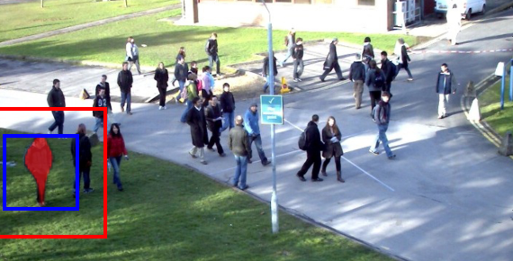
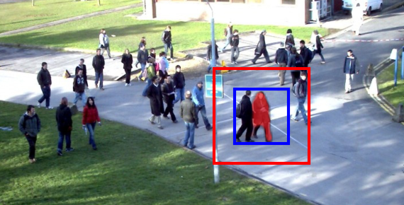
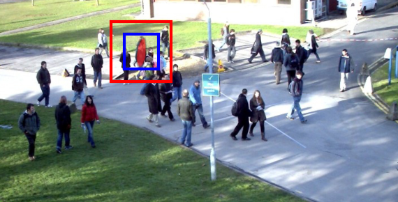
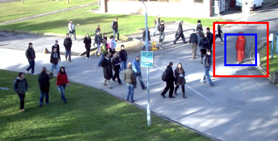
A convnet for non-maximum suppression

Abstract

Non-maximum suppression (NMS) is used in virtually all state-of-the-art object detection pipelines. While essential object detection ingredients such as features, classifiers, and proposal methods have been extensively researched surprisingly little work has aimed to systematically address NMS. The de-facto standard for NMS is based on greedy clustering with a fixed distance threshold, which forces to trade-off recall versus precision. We propose a convnet designed to perform NMS of a given set of detections. We report experiments on a synthetic setup, and results on crowded pedestrian detection scenes. Our approach overcomes the intrinsic limitations of greedy NMS, obtaining better recall and precision.

1 Introduction

The bulk of current object detection pipelines are based on three steps: 1) propose a set of windows (either via sliding window, or object proposals), 2) score each window via a properly trained classifier, 3) remove overlapping detections (non-maximum suppression). The popular DPM (Felzenszwalb et al., 2010) and R-CNN family (Girshick et al., 2014; Girshick, 2015; Ren et al., 2015) follow this approach. Both object proposals (Hosang et al., 2015) and detection classifiers (Russakovsky et al., 2015) have received enormous attention, while non-maximum suppression (NMS) has been seldom addressed. The de-facto standard for NMS consists of greedily merging the higher scoring windows with lower scoring windows if they overlap enough (e.g. intersection-over-union $\mbox{IoU}>0.5$), which we call GreedyNMS in the following.

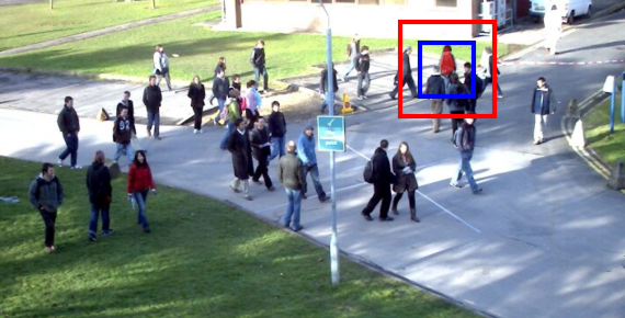
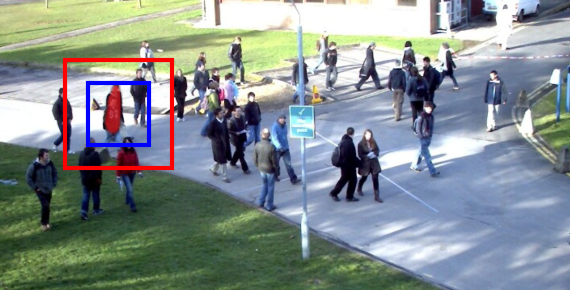
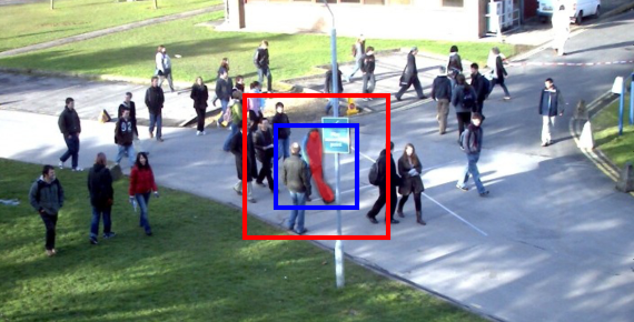
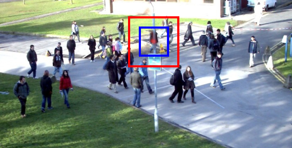
GreedyNMS is popular because it is conceptually simple, fast, and for most tasks results in satisfactory detection quality. Despite its popularity, GreedyNMS has important shortcomings. As illustrated in figure 1 (and also shown experimentally in section 4) GreedyNMS trades off precision vs. recall. If the IoU threshold is too large (too strict) then not enough surrounding detections are suppressed, high scoring false positives are introduced and precision suffers; if the IoU threshold is too low (too loose) then multiple true positives are merged together and the recall suffers (right-most case in figure 1). For any IoU threshold, GreedyNMS is sacrificing precision or recall. One can do better than this by leveraging the full signal of the score map (statistics of the surrounding detections) rather than blindly applying a fixed policy everywhere in the image.

Figure 1: 1D illustration of the GreedyNMS shortcomings. Black dots indicate true objects, grey curve is the detector response, green dots are true positives, red dots/circles are false positives/negatives. Whenever the merge criterion is too narrow false positives will be introduced (low precision, middle case), when the merge criterion is too wide there are missed detections (low recall, right case). A fixed merging criterion is doomed to fail across different situations.

Current object detectors are becoming surprisingly effective on both general (e.g. Pascal VOC, MS COCO) and specific objects detection (e.g pedestrians, faces). The oracle analyses for “perfect NMS” from Hosang et al. (2015, table 5) and Parikh & Zitnick (2011, figure 12) both indicate that NMS accounts for almost a quarter of the remaining detection problem.

GreedyNMS is, strictly speaking, not a “non-maximum suppression” method since it focuses on removing overlapping detections, ignoring if a detection is a local maximum or not. To improve detections, we would like to prune false positives (and keep true positives). Instead of doing hard pruning decisions, we design our network to make soft decisions by re-scoring (re-ranking) the input detection windows. Our re-scoring is final, and no post-processing is done afterwards, thus the resulting score maps must be very “peaky”. We call our proposed network “Tyrolean network”, abbreviated Tnet.

Contribution

We are the first to show that a convnet can be trained and used to overcome the limitations of GreedyNMS. Our experiments demonstrate that, across different occlusion levels, the Tyrolean network (Tnet) performs strictly better than GreedyNMS at any IoU threshold.

As an interesting scenario for NMS, we report results over crowded pedestrian scenes. Our Tnet is focused on the NMS task, it does not directly access image content (thus does not act as “second detector”), does not use external training data, and provides better results than auto-context (Tu & Bai, 2010).

1.1 Related work

Despite being a core ingredient of detection, non-maximum suppression has received little attention compared to feature design, classifier design, and object proposals.

Clustering detections

The decade old greedy NMS (GreedyNMS) is used in popular detectors such as V&J (Viola & Jones, 2004), DPM (Felzenszwalb et al., 2010), and is still used in the state-of-the-art R-CNN detector family (Girshick et al., 2014; Girshick, 2015; Ren et al., 2015). Alternatives such as mean-shift clustering (Dalal & Triggs, 2005; Wojek et al., 2008), agglomerative clustering (Bourdev et al., 2010), and heuristic variants (Sermanet et al., 2014) have been considered, but they have yet to show consistent gains. Recently Tang et al. (2015); Rothe et al. (2015) proposed principled clustering approaches that provide globally optimal solutions, however the results reached are on par, but do not surpass, GreedyNMS.

Linking detections to pixels

The Hough voting framework enables more sophisticated reasoning amongst conflicting detections by linking the detections to local image evidence (Leibe et al., 2008; Barinova et al., 2012; Wohlhart et al., 2012). Hough voting itself, however, provides low detection accuracy. Yao et al. (2012) and Dai et al. (2015) refine detections by linking them with semantic labelling; while Yan et al. (2015) side-steps NMS all-together by defining the detection task directly as a labelling problem. These approaches arguably propose a sound formulation of the detection problem, however they rely on semantic labelling/image segmentation. Our system can operate directly on bounding box detections.

Co-occurrence

To better handle dense crowds or common object pairs, it has been proposed to use specialized 2-object detectors (Sadeghi & Farhadi, 2011; Tang et al., 2012; Ouyang & Wang, 2013), which then require a more careful NMS strategy to merge single-object with double-object detections. Similarly Rodriguez et al. (2011) proposed to adapt the NMS threshold using crowd density estimation. Our approach is directly learning based (no hand-crafted 2-objects or density estimators), and does not use additional image information.
Desai et al. (2011) considered improving the NMS procedure by considering the spatial arrangement between detections of different classes. The feature for spatial arrangement are fully hand-crafted, while we let a convnet learn the spatial arrangement patterns. We focus here on the single class case (albeit our approach could be extended to handle multiple classes).

Speed

Neubeck & Van Gool (2006) discuss how to improve NMS speed, without aiming to improve quality. Here we aim at improving quality, while still having practical speeds.

Auto-context

uses the local (Tu & Bai, 2010; Chen et al., 2013) or global information (Vezhnevets & Ferrari, 2015) on the image to re-score detections. Albeit such approaches do improve detection quality, they still require a final NMS processing step. Our convnet does re-score detections, but at the same time outputs a score map that does not require further processing. We provide experiments (section 4) that show improved performance over auto-context.

Convnets and NMS

Recently a few works have linked convnets and NMS. Detection convnets are commonly trained unaware of the NMS post-processing step; Wan et al. (2015) connected NMS with the loss to train the detection convnet, making the training truly end-to-end. The used NMS is greedy and with fixed parameters. Stewart & Andriluka (2015) propose to use an LSTM to decide how many detections should be considered in a local region. The detections amongst the regions are then merged via traditional NMS. In contrast our convnet runs in a fully convolutional mode and requires no post-processing. Both Wan et al. (2015) and Stewart & Andriluka (2015) served as inspiration for the design of our training loss. To the best of our knowledge our Tnet is the first network explicitly designed to replace the final NMS stage.
This work focuses on NMS itself, our proposed network is independent of the detections source (it can be from a convnet or not). We report experiment applied over DPM (Felzenszwalb et al., 2010) detections.

2 Base Tyrolean network

The main intuition behind our proposed Tyrolean network (Tnet) is that the score map of a detector together with a map that represents the overlap between neighbouring hypotheses contains valuable information to perform better NMS than GreedyNMS (also see figure 1). Thus, our network is a traditional convnet but with access to two slightly unusual inputs (described below), namely score map information and IoU maps. Figure 2 shows the overall network. The parameter range (number of layers, number of units per layer) is inspired by AlexNet (Krizhevsky et al., 2012) and VGG (Simonyan & Zisserman, 2015). In our base Tnet the first stage applies $512$ $11\times 11$ filters over each input layer, and $512$ $1\times 1$ filters are applied on layers 2, 3, and 4. ReLU non-linearities are used after each layer but the last one.

The network is trained and tested in a fully convolutional fashion. It uses the same information as GreedyNMS, and does not access the image pixels directly. The required training data are only a set of object detections (before NMS), and the ground truth bounding boxes of the dataset.

Figure 2: Base architecture of our Tyrolean network (Tnet). See text for the variants considered. Each grey box is a feature map, its dimensions are indicated at its bottom, the coloured square indicates the convolutional filters size, the stride is marked next to the downward arrow. Unless indicated each layer uses ReLu non-linearities. No max-pooling nor local normalization is used. Any other processing marked in grey text.

Input grid

As preprocessing all detections in an image are mapped into a 2d grid (based on their centre location). If more than one detection falls into the same cell, we keep only the highest scoring detection. Each cell in the grid is associated with a detection bounding box and score. We use cells of $4\times 4\ \mbox{pixels}$, thus an input image of size $\mbox{W}\times\mbox{H}$ will be mapped to input layers of size $\mbox{w}\times\mbox{h}=\nicefrac{{\mbox{W}}}{{4}}\times\nicefrac{{\mbox{\mbox{H}}}}{{4}}$. Since the cells are small, mapping detections to the input grid has minimal impact on the NMS procedure. In preliminary experiments we validated that: a) we can at least recover the performance of GreedyNMS (applying GreedyNMS over the input grid provides the same results as directly applying GreedyNMS), b) the detection recall stays the same (after mapping to the input grid the overall recall is essentially identical to the raw detections).
The current incarnation of Tnet can handle mild changes in scale amongst neighbouring detections. We report experiments with detections over a $3\times$ scale range (most boxes have $[50,\,150]\ \mbox{pixel}$ height). The overall approach can handle a wider range of scale differences with simple modifications (making the grid 3d, i.e. x-y-scale), which is left for future work.

IoU layer

In order to reason about neighbouring detection boxes (or segments) we feed Tnet with IoU values. For each location we consider a $11\times 11=121$ neighbourhood, thus the input IoU layer has $\mbox{w}\times\mbox{h}\times 121$ values. Together the cell size and neighbourhood size should provide the Tnet with sufficient information about surroundings of a detection, where this choice depends on the object sizes in the image and the expected object density and thus are application dependent.

Score maps layer

To reason about the detection confidence, we feed Tnet with the raw detection score map (once mapped to the input grid). The NMS task involves ranking operations which are not easily computed by linear and relu ($\max(\cdot,\,0)$) operators. To ease the task we also feed the Tnet with score maps resulting from GreedyNMS at multiple IoU thresholds. All score maps are stacked as a multi-channel input image and feed into the network. $\mbox{S}\negthinspace\left(\tau\right)$ denotes a score map resulting from applying GreedyNMS with IoU$\geq\tau$, $\mbox{S}\negthinspace\left(\tau_{1},\,\tau_{2}\right)$ denotes a two channels map ($\mbox{S}\negthinspace\left(\tau_{1}\right)$ and $\mbox{S}\negthinspace\left(\tau_{2}\right)$ stacked). Note that $\mbox{S}\negthinspace\left(1\right)$ returns the raw detection score map. Our base Tnet uses $\mbox{S}\negthinspace\left(1,\,0.3\right)$ which has dimensionality $\mbox{w}\times\mbox{h}\times 2$ (see figure 2). The convolutional filters applied over the score maps input have the same size as the IoU layer neighbourhood ($11\times 11\ \mbox{cells}$).

Tnet is then responsible for interpreting the multiple score maps and the IoU layer, and make the best local decision. Our Tnet operates in a fully feed-forward convolutional manner. Each location is visited only once, and the decision is final. In other words, for each location the Tnet has to decide if a particular detection score corresponds to a correct detection or will be suppressed by a neighbouring detection in a single feed-forward path.

Parameter rules of thumb

Figure 2 indicates the base parameters used. Preliminary experiments indicated that removing some of the top layers has a clear negative impact on the network performance, while the width of these layers is not that important ($512$, $1\,024$, $2\,048$ filters in layers 2,3, and 4 shows a slow increase in quality). Having a high enough resolution in the input grid is critical, while keeping a small enough number of convolutions over the inputs allows to keep the number of model parameters under control. During training data augmentation is necessary to avoid overfitting. The training procedure is discussed in more detail in 2.1, while experimental results for some parameters variants are reported in section 4.

Input variants

In the experiments in the next sections we consider different input variants. The IoU layer values can be computed over bounding boxes (regressed by the sliding window detector), or over estimated instance segments (Pinheiro et al., 2015).
Similarly, for the score maps we consider different numbers of GreedyNMS thresholds, which changes the dimensionality of the input score map layer.
In all cases we expect the Tnet to improve over a fixed threshold GreedyNMS by discovering patterns in the detector score maps and IoU arrangements that enable to do adaptive NMS decisions.

2.1 Training procedure

Typically detectors are trained as classifiers on a set of positive and negative windows, determined by the IoU between detection and object annotation. When doing so the spatial relation between detector outputs and the annotations is being neglected and little work has addressed this.The DPM (Felzenszwalb et al., 2010; Pepik et al., 2015) includes structured output learning to ensure the detection score falls off linearly with the overlap between detector window and annotation. Wan et al. (2015) explicitly include a fixed NMS procedure into the network loss during training so the detector is tuned towards the NMS at test time. We adopt from Stewart & Andriluka (2015) the idea of computing the loss by matching detections to annotations, but instead of regressing bounding boxes at every location we predict new detection scores that are high for matched detections and low everywhere else. In contrast to the conventional wisdom of training the detector to have a smooth score decrease around positive instances, we declare a detection right next to a true positive to be a negative training sample as long as it is not matched to an annotation. We do this because our network must itself perform NMS.

Training loss

Our goal is to reduce the score of all detections that belong to the same person, except exactly one of them. To that end, we match every annotation to all detections that overlap at least $0.5$ IoU and choose the maximum scoring detection among them as the one positive training sample. All other detections are negative training examples. This yields a label $y_{p}$ for every location $p$ in the input grid (see previous section). Since background detections are much more frequent than true positives, it is necessary to weight the loss terms to balance the two. We use the weighted logistic loss

$$L(\mathbf{x})=\frac{1}{\sum_{p\in G}w_{y_{p}}}\sum_{p\in G}w_{y_{p}}\log\left(1+e^{-y_{p}f(x_{p})}\right)$$ (1)

where $x_{p}$ is the feature descriptor at position $p$, $f(x_{p})$ is the output of the network at position $p$. The weights $w_{y_{p}}$ are chosen so that both classes have the same weight either per frame or globally on the entire dataset (denoted by $w_{f}$ and $w_{g}$ respectively). Since we have a one-to-one correspondence between input grid cells and labels it is straight forward to train a fully convolutional network to minimize this loss.

Relaxed loss

It is impossible for the network to recover from certain mistakes that are already present in the input detections. For example, false positives on the background might be impossible to tell apart from true positives since the network does not have access to the image and only sees detection scores and overlaps between detections. On the other hand detections of distinct objects with high overlap can be hard to detect since the detections can assign low scores to barely visible objects. It proved beneficial to assign lower weight to these cases, which we call the relaxed loss. We declare negative samples to be hard if the corresponding detections are not suppressed by a 0.3 NMS and true positives to be hard if they are suppressed by a 0.3 NMS on the annotations with the matched detection scores. The weight of hard examples is decreased by a factor of $r$. Our base Tnet uses $r=1$ (non-relaxed) with weighting strategy $w_{f}$, and section 4 reports results for other $r$ values and $w_{g}$.

Training parameters

The model is trained from scratch, randomly initialized with MSRA (He et al., 2015), and optimized with Adam (Kingma & Ba, 2015). We use a learning rate of $10^{-4}$, a weight decay of $5\cdot 10^{-5}$, a momentum of 0.9, and gradient clipping at $1\,000$. The model is trained for $100\,000$ iterations with one image per iteration. All experiments are implemented with the Caffe framework (Jia et al., 2014).

As pointed out in Mathias et al. (2014) the threshold for GreedyNMS requires to be carefully selected on the validation set of each task, the commonly used default $\mbox{IoU}>0.5$ can severely underperform. Other NMS approaches such as (Tang et al., 2015; Rothe et al., 2015) also require training data to be adjusted. When maximizing performance in cluttered scenes is important, training a Tnet is thus not a particularly heavy burden. Currently, training our base Tnet on un-optimized CPU and GPU code takes a day.

3 Controlled setup experiments

NMS is usually the last stage of an entire detection pipeline. Therefore, in an initial set of experiments, we want to understand the problem independent of a specific detector and abstract away the particularities of a given dataset.

3.1 oMNIST dataset

If all objects appeared alone in the images, NMS would be trivial. The core issue for NMS is deciding if two local maxima in the detection score map correspond to only one object or to multiple ones. To investigate this core aspect we create the oMNIST (“overlapping MNIST”) toy dataset. This data does not aim at being particularly realistic, but rather to enable a detailed analysis of the NMS problem.

Image
Score map

Figure 3: Example data from our controlled experiments setup. The convnet must decide if one or two digits are present (and predict is their exact location) while using only a local view of score and IoU maps (no access to the input image).

Each image is composed of one or two MNIST digits. To emphasise the occlusion cases, we sample $\nicefrac{{1}}{{5}}$ single digits, and $\nicefrac{{4}}{{5}}$ double digit cases. The digits are off-centre and when two digits are present they overlap with bounding box $\mbox{IoU}\in[0.2,\,0.6]$. We also mimic a detector by generating synthetic score maps. Each ground truth digit location generates a perturbed bump with random magnitude in the range $[1,\,9]$, random x-y scaling, rotation, a small translation, and additive Gaussian noise. Albeit noisy, the detector is “ideal” since its detection score remains high despite strong occlusions. Figure 3 shows examples of the generated score maps and corresponding images. By design GreedyNMS will have difficulties handling such cases (at any IoU threshold).

Other than score maps our convnet uses IoU information between neighbouring detections (like GreedyNMS). In our experiments we consider using the perfect segmentation masks for IoU (ideal case), noisy segmentation masks, and the sliding window bounding boxes.

Image
Score map
GreedyNMS
Tnet

Figure 4: Example score maps on the oMNIST dataset. First to last row: Image, input score map, GreedyNMS $\mbox{IoU}>0.3$, and Tnet $\mbox{IoU}\,\&\,\mbox{S}\negthinspace\left(1,\,0\rightarrow 0.6\right)$. GreedyNMS produces false positives and prunes true positives, while Tnet correctly localize even very close digits.

We generate a training/test split of $100\mbox{k}$/$10\mbox{k}$ images, kept fix amongst different experiments.

3.2 Results

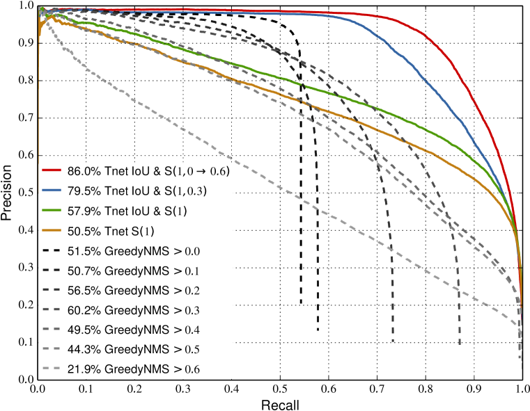
Results are summarised in table 1 and figure 5. We summarise the curves via AR; the average recall on the precision range $[0.5,\,1.0]$. The evaluation is done using the standard Pascal VOC protocol, with $\mbox{IoU}>0.5$ (Everingham et al., 2015).

GreedyNMS

As can be easily seen in figure 5 varying the IoU thresholds for GreedyNMS trades off precision and recall as discussed in section 1. The best AR that can be obtained with GreedyNMS is $60.2\%$ for $\mbox{IoU}>0.3$. Example score maps for this method can be found in figure 4.

Upper bound

As an upper bound for any method relying on score map information we can calculate the overlap between neighbouring hypotheses based on perfect segmentation masks available in this toy scenario. In that case even a simple strategy such as GreedyNMS can be used and based on our idealized but noisy detection score maps this results in $90.0\%\ \mbox{AR}$. In section 4 we report experiments using segmentation masks estimated from the image content that result in inferior performance however.

Figure 5: Detection results on controlled setup (oMNIST test set).

Table 1: Results from controlled setup experiments. $\mbox{S}\left(\cdot\right)$ indicates the different input score maps.

Method	AR
Upper bound
perfect masks	90.0%
GreedyNMS
bboxes $\mbox{IoU}>0.3$	60.2%
Tnet
$\mbox{IoU}\,\&\,\mbox{S}\negthinspace\left(1,\,0\rightarrow 0.6\right)$	86.0%
$\mbox{IoU}\,\&\,\mbox{S}\negthinspace\left(1,\,0.3\right)$	79.5%
$\mbox{IoU}\,\&\,\mbox{S}\negthinspace\left(1\right)$	57.9%
$\mbox{S}\negthinspace\left(1\right)$	50.5%

Base Tnet

Using the same information as GreedyNMS with bounding boxes, our base Tnet reaches better performance for the entire recall range (see figure 5 and table 1, $\mbox{S}\negthinspace\left(1,\,0.3\right)$ indicates the score maps from GreedyNMS with $\mbox{IoU}>0.3$ and $\geq 1$, i.e. the raw score map). In this configuration Tnet obtains $79.5\%\ \mbox{AR}$ clearly superior to GreedyNMS. This shows that, at least in a controlled setup, a convnet can indeed exploit the available information to overcome the limitations of the popular GreedyNMS method.

Instead of picking a specific IoU threshold to feed Tnet, we consider $\mbox{IoU}\,\&\,\mbox{S}\negthinspace\left(1,\,0\rightarrow 0.6\right)$, which includes $\mbox{S}\negthinspace\left(1,\,0.6,\,0.4,\,0.3,\,0.2,\,0.0\right)$. As seen in figure 5, not selecting a specific threshold results in the best performance of $86.0\%\ \mbox{AR}$. As soon as some ranking signal is provided (via GreedyNMS results), our Tnet is able to learn how to exploit best the information available. Qualitative results are presented in figure 4.

Table 1 reports results for a few degraded cases. If we remove GreedyNMS $\mbox{S}\negthinspace\left(0.3\right)$ and only provide the raw score map ($\mbox{IoU}\,\&\,\mbox{S}\negthinspace\left(1,\,0.3\right)$) performance decreases somewhat.

Auto-context

Importantly we show that $\mbox{IoU}\,\&\,\mbox{S}\negthinspace\left(1\right)$ improves over $\mbox{S}\negthinspace\left(1\right)$ only. ($\mbox{S}\negthinspace\left(1\right)$ is the information exploited by auto-context methods, see §1.1). This shows that the convnet is learning to do more than simple auto-context. The detection improves not only by noticing patterns on the score map, but also on how the detection boxes overlap.

4 Person detection experiments

After the proof of concept for a controlled setup, we move to a realistic pedestrian detection setup. We are particularly interested in datasets that show diverse amounts of occlusion (and thus NMS is non-trivial). We decided for the PETS dataset, which exhibits diverse levels of occlusion and provides a reasonable volume of training and test data. Additionally we test the generalization of the trained model on the ParkingLot dataset.

Figure 6: Distribution of overlap between ground truth PETS and ParkingLot annotations (measured in IoU). Most persons on the datasets have some occlusion, and about $\sim\negmedspace 20\%$ have significant occlusion ($\mbox{IoU}>0.4$).

PETS

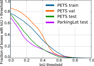
We use 8 of the PETS sequences (Ferryman & Ellis, 2010), $\sim\negmedspace 200$ frames each, that we split in 5 for training (S1L1-1, S1L1-2, S1L2-1, S1L2-2, S2L1, and S3MF1), 1 for validation (S2L3) and 1 for testing (S2L2). The different videos show diverse densities of crowds. As shown in figure 6 more than $40$/$50$/$25\%$ of the train/val/test data has an $\mbox{IoU}>0.3$ with another ground truth box.
Since detectors tend to have non-zero detection scores in most areas of the image, the training volume is proportional to number of pixels not the number of images. Thus we can adequately train our Tnet with only a few hundred frames.
PETS has been previously used to study person detection (Tang et al., 2013), tracking (Milan et al., 2014), and crowd density estimation (Subburaman et al., 2012). Standard pedestrian datasets such as Caltech (Dollár et al., 2012) or KITTI Geiger et al. (2012) average less than two pedestrian per frame, making close-by detections a rare occurrence.
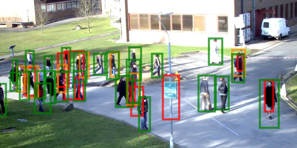
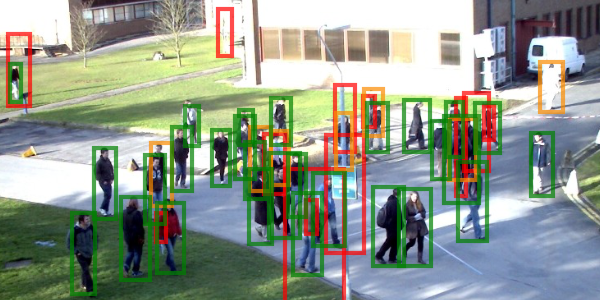
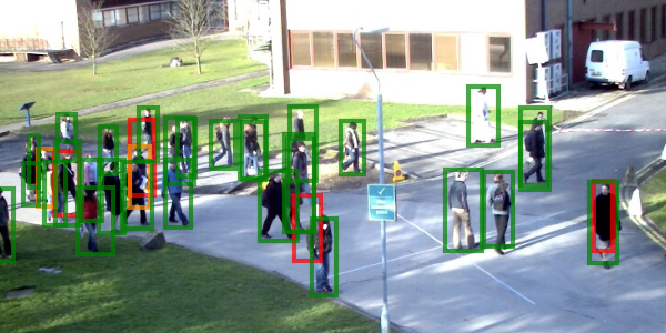
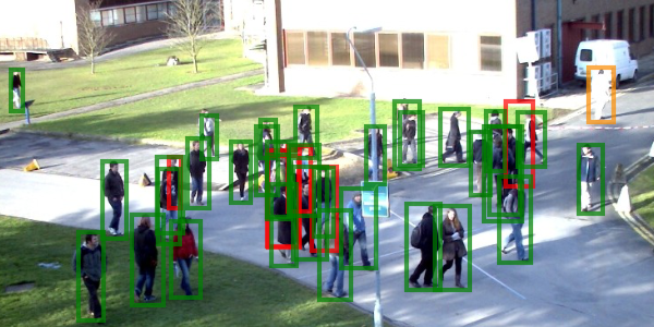
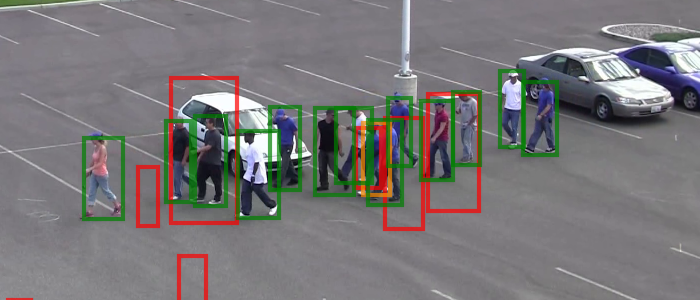
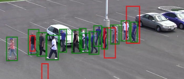
Due to its size and challenging occlusion statistics we consider PETS a suitable dataset to explore NMS. Figure 11 shows example frames.

ParkingLot

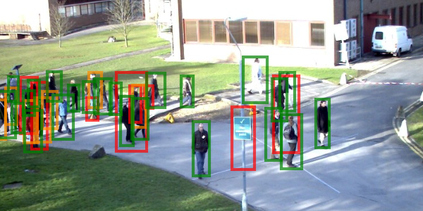
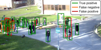
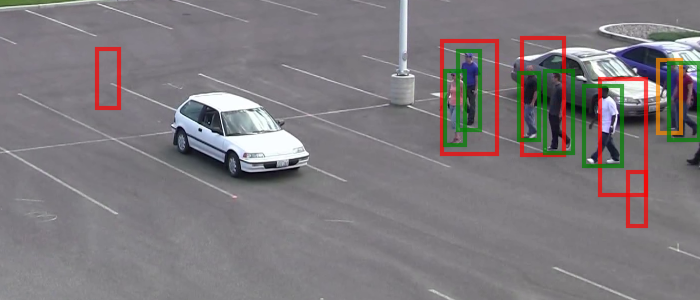
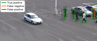
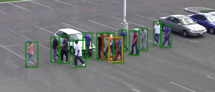
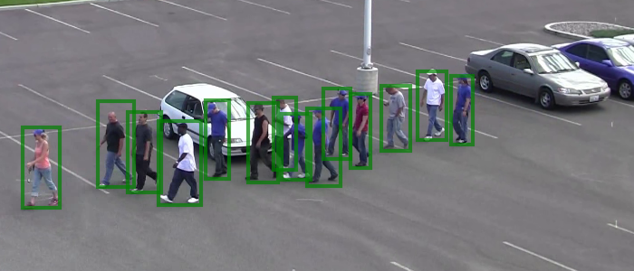
We use the first ParkingLot (Shu et al., 2012) sequence to evaluate the generalization capabilities of the model. We use an improved set annotations, provided every third frame (250 frames in total) and rectify the mistakes from the original annotations. Compared to PETS the sequence has similar overlap statistics than the PETS test set (see figure 6), but presents different background and motion patterns. Figure 12 shows examples from the dataset.

Person detector

In this work we take the detector as a given. For our experiments we use the baseline DPM detector from (Tang et al., 2013). We are not aware of a detector (convnet or not) providing better results on PETS-like sequences (we considered some of the top detectors in (Dollár et al., 2012)). Importantly, for our exploration the detector quality is not important per-se. As discussed in section 3.1 GreedyNMS suffers from intrinsic issues, even when providing an idealized detector. In fact Tnet benefits from better detectors, since there will be more signal in the score maps, it becomes easier to do NMS. We thus consider our DPM detector a fair detection input.
We use the DPM detections after bounding box regression, but before any NMS processing.

Person segments

In section 4.1 we report results using segments estimated from the image content. We use our re-implementation of DeepMask (Pinheiro et al., 2015), trained on the Coco dataset (Lin et al., 2014). DeepMask is a network specifically designed for objects segmentation which provides competitive performance. Our re-implementation obtains results of comparable quality as the original; example results on PETS are provided in the appendix section A. We use DeepMask as a realistic example of what can be expected from modern techniques for instance segmentation.

4.1 PETS results

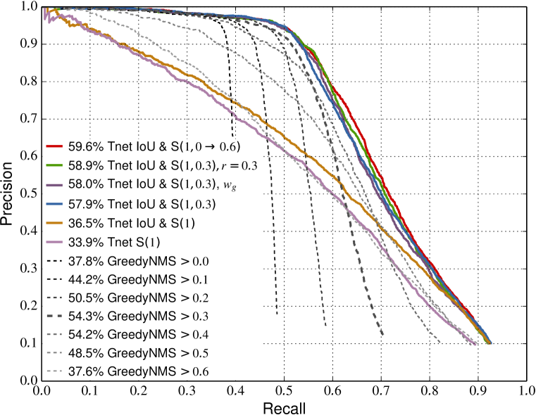
Our PETS results are presented in table 2, figure 7 (validation set), figures 9, 9 (test set). Qualitative results are shown in figure 11.

Table 2: Results on PETS validation set. Underlined is our base Tnet.

Method	AR
GreedyNMS
bboxes $\mbox{IoU}>0.3$	54.3%
DeepMask segments	52.0%
Tnet variants
$\mbox{IoU}\,\&\,\mbox{S}\negthinspace\left(1,\,0\negthinspace\rightarrow\negthinspace 0.6\right)$	59.6%
$\mbox{IoU}\,\&\,\mbox{S}\negthinspace\left(1,\,0.3\right)$, $r=0.3$	58.9%
$\mbox{IoU}\,\&\,\mbox{S}\negthinspace\left(1,\,0.3\right)$, $w_{g}$	58.0%
$\mbox{IoU}\,\&\,\mbox{S}\negthinspace\left(1,\,0.3\right)$	57.9%
$\mbox{IoU}\,\&\,\mbox{S}\negthinspace\left(1\right)$	36.5%
$\mbox{S}\negthinspace\left(1\right)$	33.9%

Figure 7: Detection results on PETS validation set. Global weighting is indicated by $w_{g}$, all other curves use frame weighting.

GreedyNMS on boxes

Just like in the oMNIST case, the GreedyNMS curves in figure 7 have a recall versus precision trade-off. For PETS we pick $\mbox{IoU}>0.3$ as a reference threshold which provides a reasonable balance.

GreedyNMS on segments

As discussed in section 3, GreedyNMS should behave best when the detection overlap is based on the visible area of the object. We compute DeepMask segmentations on the DPM detection, feed these in GreedyNMS, and select the best IoU threshold for the validation set. As seen in table 2 results are slightly under-performing the bounding boxes cases. Albeit many segments are rather accurate (see appendix section A), segments tend to be accurate on the easy cases for the detector, and drop in performance when heavier occlusion is present. Albeit in theory having good segmentations should make GreedyNMS quite better, in practice they do not. At the end, the segments hurt more than they help for GreedyNMS.

Auto-context

The entry $\mbox{S}\left(1\right)$ in table 2 shows the case where only the raw detection score map is feed to Tnet (same nomenclature as section 3.2). Since performance is lower than other variants (e.g. $\mbox{IoU}\,\&\,\mbox{S}\left(1\right)$), this shows that our approach is exploiting available information better than just doing auto-context over DPM detections.

Tnet

Both in validation and test set (figures 7 and 9) our trained network with $\mbox{IoU}\,\&\,\mbox{S}\left(1,\,0.3\right)$ input provides a clear improvement over vanilla GreedyNMS. Just like in the oMNIST case, the network is able to leverage patterns in the detector output to do better NMS than the de-facto standard GreedyNMS method.
Table 2 report the results for a few additional variants. $\mbox{IoU}\,\&\,\mbox{S}\negthinspace\left(1,\,0\rightarrow 0.6\right)$ shows that it is not necessary to select a specific IoU threshold for the input score map layer. Given an assortment ($\mbox{S}\negthinspace\left(1,\,0.6,\,0.4,\,0.3,\,0.2,\,0.0\right)$) the network will learn to leverage the information available.
Using the relaxed loss described in 2.1 helps further improve the results. Amongst the parameters tried on the validation set, $r=0.3$ provides the largest improvement. Lower $r$ values decrease performance, while higher $r$ values converge towards the default $r=1$ performance (base Tnet).
Weighting classes equally on the entire dataset ($w_{g}$ strategy) gives a mild improvement from $57.9\%$ to $58.0$% AR compared to the default per frame weighting $w_{f}$.

Figure 8: Detection results on PETS test set. Our approach is better than any GreedyNMS threshold and better than the upper envelope of all GreedyNMS curves.

Figure 9: GreedyNMS versus Strong Tnet when evaluated over different subsets of PETS test data, based on level of occlusion. In each subset our Tnet improves over the upper envelope of all GreedyNMS threshold curves.

Strong Tnet

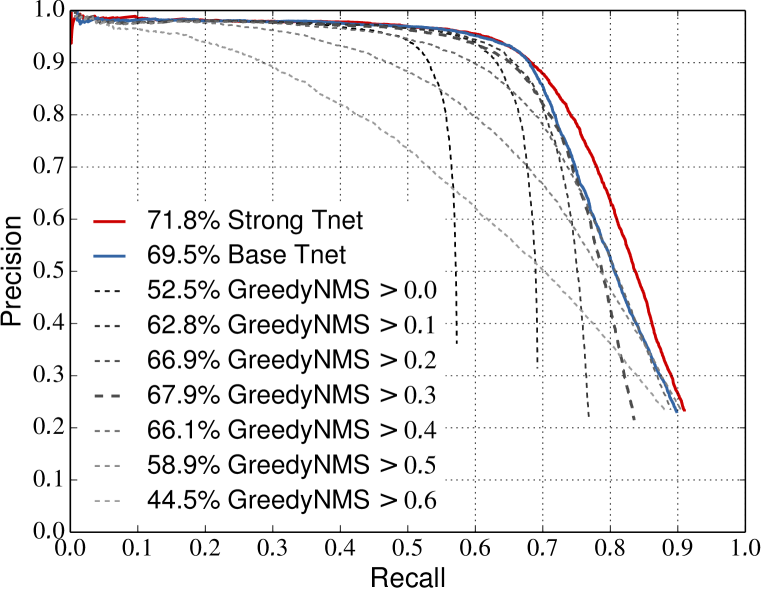
We combine the best ingredients identified on the validation set into one strong model. We use $\mbox{IoU}\,\&\,\mbox{S$\left(1,\,0\negthinspace\rightarrow\negthinspace 0.6\right)$}$, relaxed loss with $r=0.3$, and global weighting $w_{g}$. Figure 9 shows that we further improve over the base Tnet from $59.5\%$ to $71.8\%\ \mbox{AR}$ on the PETS test set. The gap between base Tnet and GreedyNMS is smaller on the test set than on validation, because test set has lighter occlusions (see figure 6). Still our strong Tnet provides a consistent improvement over GreedyNMS.
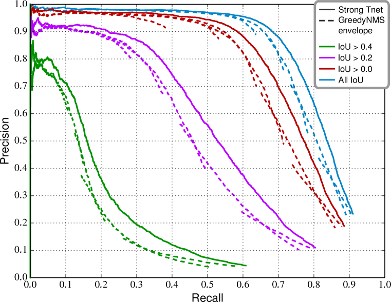
Figure 9 provides a more detailed view of the results from figure 9. It compares our strong Tnet result versus the upper envelope of GreedyNMS over all thresholds ($[0,\,1]$), when evaluated over different subsets of the test set. Each subset corresponds to ground truth bounding boxes with other boxes overlapping more than a given IoU level (see figure 6). For all ranges, our strong Tnet improves over GreedyNMS. This shows that our network does not fit to a particular range of occlusions, but learns to handle all of them with comparable effectiveness.
At test time Tnet is reasonably fast, taking $\sim\negmedspace 200\ \mbox{milliseconds}$ per frame (all included).

4.2 ParkingLot results

Figure 10: Detection results on the ParkingLot dataset. Tnet is better than any GreedyNMS threshold, even though it has been trained using PETS data only.

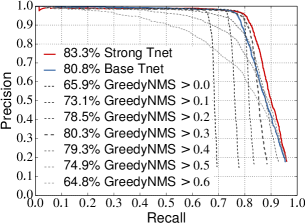
To verify that our Tnet can generalize beyond PETS, we run the same DPM detector as on the PETS experiment over the ParkingLot sequence and do NMS using the networks trained on PETS training set only. Results in figure 10 show that Tnet improves from $80.3\%$ to $83.3\%$ AR over the best GreedyNMS threshold of $\text{{IoU}}>0.3$. Even though Tnet was not trained on this sequence we see a similar result as on the PETS dataset. Not only does our Strong Tnet improve over the best GreedyNMS result, but it improves over the upper envelope of all GreedyNMS thresholds. See qualitative results in figure 12.

5 Conclusion

We have discussed in detail the limitations of GreedyNMS and presented experimental examples showing its recall versus precision trade-off. For the sake of speed and simplicity GreedyNMS disregards most of the information available in the detector response. Our proposed Tyrolean network (Tnet) mines the patterns in the score map values and bounding box arrangements to surpass the performance of GreedyNMS. On the person detection task, our final results show that our approach provides, compared to any GreedyNMS threshold, both high recall and improved precision. These results confirm that Tnet overcomes the intrinsic limitations of GreedyNMS, while keeping practical test time speeds.

Albeit the proposed architecture results in good results for the scenario covered, there is certainly room for further probing the parameter space of convnets for NMS and exploring other applications domains (e.g. NMS for boundaries estimation, or other detection datasets). Explicitly handling detection scales, considering multi-class problems, or back-propagating into the detector itself are future directions of interest.

Current detection pipelines start with a convnet and end with a hard-coded NMS procedure. For detection problems where occlusions are present, we reckon that significant improvements can be obtained by ending with a Tnet.

(a) GreedyNMS

(b) Strong Tnet

Figure 11: Qualitative detection results of GreedyNMS $>0.3$ and Strong Tnet over DPM detections on PETS test set (both operating at 75% recall). Tnet is able to suppress false positives as well as recover recall that is lost with GreedyNMS. This is the case for both crowded and non-crowded areas.

(a) GreedyNMS

(b) Strong Tnet

Figure 12: Qualitative detection results of GreedyNMS $>0.3$ and Strong Tnet over DPM detections on ParkingLot dataset (both operating at 85% recall). Tnet was trained using PETS only.

Acknowledgements

We thank Siyu Tang and Anton Milan for providing the pre-trained DPM model and additional PETS ground-truth annotations, respectively.

Supplementary material

Appendix A DeepMask results on PETS

To obtain segmentation masks on PETS, we train our reimplementation of DeepMask (Pinheiro et al., 2015) for all classes on the COCO training set. Our implementation is based on the Fast-RCNN network Girshick (2015). To generate instance segmentations on PETS, we upscale the image by a factor of $2\times$ and predict segments on detections. Figure 13 shows mask predictions for annotations on the PETS test set. It works well in low occlusion cases (left and middle column), however, under heavy occlusion it makes mistakes by collapsing the segment or merging the occluding and the occluded person (see right-most column).

Figure 13: Example DeepMask segmentation masks on PETS images. Pixels inside the red area are used to predict a foreground segment inside the blue area. In these examples, boxes are centred on ground truth annotations.

References

- Barinova et al. (2012) Barinova, Olga, Lempitsky, Victor, and Kholi, Pushmeet. On detection of multiple object instances using hough transforms. PAMI, 2012.
- Bourdev et al. (2010) Bourdev, Lubomir, Maji, Subhransu, Brox, Thomas, and Malik, Jitendra. Detecting people using mutually consistent poselet activations. In ECCV, 2010.
- Chen et al. (2013) Chen, Guang, Ding, Yuanyuan, Xiao, Jing, and Han, Tony X. Detection evolution with multi-order contextual co-occurrence. In CVPR, 2013.
- Dai et al. (2015) Dai, Jifeng, He, Kaiming, and Sun, Jian. Convolutional feature masking for joint object and stuff segmentation. In CVPR, 2015.
- Dalal & Triggs (2005) Dalal, N. and Triggs, B. Histograms of oriented gradients for human detection. In CVPR, 2005.
- Desai et al. (2011) Desai, C., Ramanan, D., and Fowlkes, C. Discriminative models for multi-class object layout. IJCV, 2011.
- Dollár et al. (2012) Dollár, Piotr, Wojek, Christian, Schiele, Bernt, and Perona, Pietro. Pedestrian detection: An evaluation of the state of the art. PAMI, 2012.
- Everingham et al. (2015) Everingham, M., Eslami, S. M. A., Van Gool, L., Williams, C. K. I., Winn, J., and Zisserman, A. The pascal visual object classes challenge: A retrospective. IJCV, 2015.
- Felzenszwalb et al. (2010) Felzenszwalb, P., Girshick, R., McAllester, D., and Ramanan, D. Object detection with discriminatively trained part-based models. PAMI, 2010.
- Ferryman & Ellis (2010) Ferryman, J and Ellis, Anna. Pets2010: Dataset and challenge. In AVSS, 2010.
- Geiger et al. (2012) Geiger, Andreas, Lenz, Philip, and Urtasun, Raquel. Are we ready for autonomous driving? the kitti vision benchmark suite. In CVPR, 2012.
- Girshick (2015) Girshick, R. Fast R-CNN. In ICCV, 2015.
- Girshick et al. (2014) Girshick, R., Donahue, J., Darrell, T., and Malik, J. Rich feature hierarchies for accurate object detection and semantic segmentation. In CVPR, 2014.
- He et al. (2015) He, Kaiming, Zhang, Xiangyu, Ren, Shaoqing, and Sun, Jian. Delving deep into rectifiers: Surpassing human-level performance on imagenet classification. In ICCV, 2015.
- Hosang et al. (2015) Hosang, Jan, Benenson, Rodrigo, Dollár, Piotr, and Schiele, Bernt. What makes for effective detection proposals? PAMI, 2015.
- Jia et al. (2014) Jia, Yangqing, Shelhamer, Evan, Donahue, Jeff, Karayev, Sergey, Long, Jonathan, Girshick, Ross, Guadarrama, Sergio, and Darrell, Trevor. Caffe: Convolutional architecture for fast feature embedding. arXiv:1408.5093, 2014.
- Kingma & Ba (2015) Kingma, D.P. and Ba, J. Adam: A method for stochastic optimization. In ICLR, 2015.
- Krizhevsky et al. (2012) Krizhevsky, A., Sutskever, I., and Hinton, G. E. Imagenet classification with deep convolutional neural networks. In NIPS, 2012.
- Leibe et al. (2008) Leibe, Bastian, Leonardis, Aleš, and Schiele, Bernt. Robust object detection with interleaved categorization and segmentation. IJCV, 2008.
- Lin et al. (2014) Lin, Tsung-Yi, Maire, Michael, Belongie, Serge, Hays, James, Perona, Pietro, Ramanan, Deva, Dollár, Piotr, and Zitnick, C Lawrence. Microsoft coco: Common objects in context. In ECCV, 2014.
- Mathias et al. (2014) Mathias, M., Benenson, R., Pedersoli, M., and Van Gool, L. Face detection without bells and whistles. In ECCV, 2014.
- Milan et al. (2014) Milan, A., Roth, S., and Schindler, K. Continuous energy minimization for multitarget tracking. PAMI, 2014.
- Neubeck & Van Gool (2006) Neubeck, Alexander and Van Gool, Luc. Efficient non-maximum suppression. In ICPR, 2006.
- Ouyang & Wang (2013) Ouyang, W. and Wang, X. Single-pedestrian detection aided by multi-pedestrian detection. In CVPR, 2013.
- Parikh & Zitnick (2011) Parikh, Devi and Zitnick, C. Human-debugging of machines. In NIPS WCSSWC, 2011.
- Pepik et al. (2015) Pepik, Bojan, Stark, Michael, Gehler, Peter, and Schiele, Bernt. Multi-view and 3d deformable part models. PAMI, 2015.
- Pinheiro et al. (2015) Pinheiro, Pedro O, Collobert, Ronan, and Dollar, Piotr. Learning to segment object candidates. In NIPS, 2015.
- Ren et al. (2015) Ren, S., He, K., Girshick, R., and Sun, J. Faster R-CNN: Towards real-time object detection with region proposal networks. In NIPS, 2015.
- Rodriguez et al. (2011) Rodriguez, Mikel, Laptev, Ivan, Sivic, Josef, and Audibert, Jean-Yves. Density-aware person detection and tracking in crowds. In ICCV, 2011.
- Rothe et al. (2015) Rothe, Rasmus, Guillaumin, Matthieu, and Van Gool, Luc. Non-maximum suppression for object detection by passing messages between windows. In ACCV, 2015.
- Russakovsky et al. (2015) Russakovsky, Olga, Deng, Jia, Su, Hao, Krause, Jonathan, Satheesh, Sanjeev, Ma, Sean, Huang, Zhiheng, Karpathy, Andrej, Khosla, Aditya, Bernstein, Michael, Berg, Alexander C., and Fei-Fei, Li. ImageNet Large Scale Visual Recognition Challenge. IJCV, 2015.
- Sadeghi & Farhadi (2011) Sadeghi, M. A. and Farhadi, A. Recognition using visual phrases. In CVPR, 2011.
- Sermanet et al. (2014) Sermanet, Pierre, Eigen, David, Zhang, Xiang, Mathieu, Michael, Fergus, Rob, and LeCun, Yann. Overfeat: Integrated recognition, localization and detection using convolutional networks. In ICLR, 2014.
- Shu et al. (2012) Shu, Guang, Dehghan, Afshin, Oreifej, Omar, Hand, Emily, and Shah, Mubarak. Part-based multiple-person tracking with partial occlusion handling. In CVPR, 2012.
- Simonyan & Zisserman (2015) Simonyan, K. and Zisserman, A. Very deep convolutional networks for large-scale image recognition. In ICLR, 2015.
- Stewart & Andriluka (2015) Stewart, Russell and Andriluka, Mykhaylo. End-to-end people detection in crowded scenes. arXiv:1506.04878, 2015.
- Subburaman et al. (2012) Subburaman, Venkatesh Bala, Descamps, Adrien, and Carincotte, Cyril. Counting people in the crowd using a generic head detector. In AVSS, 2012.
- Tang et al. (2012) Tang, S., Andriluka, M., and Schiele, B. Detection and tracking of occluded people. In BMVC, 2012.
- Tang et al. (2013) Tang, Siyu, Andriluka, Mykhaylo, Milan, Anton, Schindler, Kaspar, Roth, Stefan, and Schiele, Bernt. Learning people detectors for tracking in crowded scenes. In ICCV, 2013.
- Tang et al. (2015) Tang, Siyu, Andres, Bjoern, Andriluka, Mykhaylo, and Schiele, Bernt. Subgraph decomposition for multi-target tracking. In CVPR, 2015.
- Tu & Bai (2010) Tu, Zhuowen and Bai, Xiang. Auto-context and its application to high-level vision tasks and 3d brain image segmentation. PAMI, 2010.
- Vezhnevets & Ferrari (2015) Vezhnevets, Alexander and Ferrari, Vittorio. Object localization in imagenet by looking out of the window. In BMVC, 2015.
- Viola & Jones (2004) Viola, P. and Jones, M. Robust real-time face detection. In IJCV, 2004.
- Wan et al. (2015) Wan, Li, Eigen, David, and Fergus, Rob. End-to-end integration of a convolutional network, deformable parts model and non-maximum suppression. In CVPR, 2015.
- Wohlhart et al. (2012) Wohlhart, Paul, Donoser, Michael, Roth, Peter M., and Bischof, Horst. Detecting partially occluded objects with an implicit shape model random field. In ACCV, 2012.
- Wojek et al. (2008) Wojek, Christian, Dorkó, Gyuri, Schulz, André, and Schiele, Bernt. Sliding-windows for rapid object class localization: A parallel technique. In DAGM, 2008.
- Yan et al. (2015) Yan, Junjie, Yu, Yinan, Zhu, Xiangyu, Lei, Zhen, and Li, Stan Z. Object detection by labeling superpixels. In CVPR, 2015.
- Yao et al. (2012) Yao, J., Fidler, S., and Urtasun, R. Describing the scene as a whole: Joint object detection, scene classification and semantic segmentation. In CVPR, 2012.