Neutrino Anarchy and Renormalization Group Evolution

Vedran Brdar1 vbrdar@uni-mainz.de    Matthias König1 m.koenig@uni-mainz.de    Joachim Kopp1 jkopp@uni-mainz.de 1 PRISMA Cluster of Excellence and Mainz Institute for Theoretical Physics,
Johannes Gutenberg-Universität Mainz, 55099 Mainz, Germany
(March 7, 2024)
Abstract

The observed pattern of neutrino mixing angles is in good agreement with the hypothesis of neutrino anarchy, which posits that Nature has chosen the entries of the leptonic mixing matrix at random. In this paper we investigate how stable this conclusion is under renormalization group effects. Working in the simplest type-I seesaw model and two variants of the inverse seesaw model we study how the statistical distributions of the neutrino mixing parameters evolve between the Grand Unification scale and the electroweak scale. Especially in the inverse seesaw case we find significant distortions: mixing angles tend to be smaller after RG running, and the Dirac CP phase tends to be closer to zero. The p𝑝p-value describing the compatibility between the observed mixing angles and the anarchy hypothesis increases by 10–20%. This illustrates that RG effects are highly relevant for quantitative studies of the anarchy scenario.

pacs:
preprint: MITP/15-104

I Introduction

The flavor structure of leptons in the Standard Model (SM) is experimentally well established, but our theoretical understanding of its origin is very poor. The simplest postulate is that there is no particular structure to the neutrino mass matrix, but that its elements are randomly chosen 𝒪(1)𝒪1\mathcal{O}(1) parameters. This scenario is called neutrino anarchy [1, 2]. While one may view the idea of nature choosing model parameters at random with some reservation, it does not seem so unnatural given that nature also chooses the outcome of quantum mechanical measurements at random. Moreover, it can be considered a valid low-energy description if the underlying UV-complete theory is sufficiently complicated [2].

Once we accept the idea of anarchy, it can be used to derive meaningful predictions for the values of the neutrino mixing parameters. In particular, as shown in [2], the requirement that different elements of the mass matrices are statistically independent and that their distributions are basis-independent leads uniquely to the conclusion that the lepton mixing matrix UPMNSsubscript𝑈PMNSU_{\text{PMNS}} must have a flat distribution in the Haar measure of the U(3)𝑈3U(3) group. This allows one to compute p𝑝p-values for the experimentally measured mixing parameters [2, 3, 4, 5]. The original neutrino anarchy scenario [1] has been criticized in [4] on the grounds that it cannot be formulated unambiguously if mass matrices that only differ in their unphysical phases are considered identical. This viewpoint is valid if one assumes that nature does not “know” about the unphysical phases at all, i.e. that they do not appear as hidden variables in the theory. It becomes invalid if we accept the unphysical phases as equipollent with the physical ones, for instance on the grounds that they might have physical significance in an underlying UV-complete theory.

Of course the idea of anarchy is not restricted to the neutrino mass models in which it was originally proposed, but has also been applied for instance to scenarios with sterile neutrinos [6, 7], models with extra dimensions [8], and in the context of grand unified theories (GUTs) [9, 10, 11]. Moreover, the idea that physical parameters are drawn from a statistical distribution has received some attention in the context of the string landscape, see for instance [12, 13].

In this paper we investigate how stable the predictions of neutrino anarchy are under the effects of renormalization group (RG) running. This is an important question given that we do not know how and at what scale the random selection of model parameters happens. It could be a feature of a grand unified theory, of quantum gravity, or it could be an outcome of the dynamics at the end of inflation. We will show that in the simplest type-I seesaw scenario, which augments the SM by three heavy right-handed neutrinos, mixing angles derived from anarchical mass matrices at a high energy scale can differ from those at experimentally testable scales by several degrees. The probability of the neutrino oscillation parameters being at their experimentally observed values under the anarchy hypothesis increases by 7%similar-toabsentpercent7\sim 7\% because of this. We show that this result does not depend on the statistical test we choose to make the comparison. We also investigate how our results change in extended neutrino mass models. In particular, we show that renormalization group effects become larger in inverse seesaw models.

The plan of the paper is as follows: In section II, we will review neutrino anarchy and its predictions without including renormalization group effects. Comparing these predictions to data quantitatively, we will show that results are robust with respect to the choice of statistical test. Section III contains our main results: we will investigate how the predictions of neutrino anarchy are modified when renormalization group running from the GUT breaking scale MGUT1016similar-tosubscript𝑀GUTsuperscript1016M_{\text{GUT}}\sim 10^{16} GeV to the electroweak scale is taken into account. We will do this for the type-I seesaw scenario (section III.1), for the phenomenological inverse seesaw model (section III.2), and for a particular realization of the inverse seesaw model involving a gauged U(1)BL𝑈subscript1𝐵𝐿U(1)_{B-L} symmetry (section III.3). Besides looking at the mixing angles and complex phases, we will also study the predictions that neutrino anarchy makes for the effective neutrino mass parameter probed in searches for neutrinoless double beta (0ν2β0𝜈2𝛽0\nu 2\beta) decay. We will present our conclusions in section IV. In the appendices, we will offer details on the renormalization group equations we employ. In particular for the inverse seesaw model with U(1)BL𝑈subscript1𝐵𝐿U(1)_{B-L} symmetry, these equations have, to the best of our knowledge, not been presented before.

II Neutrino Anarchy

II.1 Statistical tests

We consider first the type-I seesaw scenario, where the SM is extended by adding three right-handed singlet fermions NRαsuperscriptsubscript𝑁𝑅𝛼N_{R}^{\alpha}. The relevant terms in the Lagrangian are

type-IYeαβeRα¯HLβYναβNRα¯H~Lβ12MαβNα¯(Nβ)c+h.c.,formulae-sequencesuperscriptsubscript𝑌𝑒𝛼𝛽¯superscriptsubscript𝑒𝑅𝛼superscript𝐻superscript𝐿𝛽superscriptsubscript𝑌𝜈𝛼𝛽¯superscriptsubscript𝑁𝑅𝛼superscript~𝐻superscript𝐿𝛽12superscript𝑀𝛼𝛽¯superscript𝑁𝛼superscriptsuperscript𝑁𝛽𝑐subscripttype-I𝑐\displaystyle\mathcal{L}_{\text{type-I}}\supset-Y_{e}^{\alpha\beta}\overline{e_{R}^{\alpha}}H^{\dagger}L^{\beta}-Y_{\nu}^{\alpha\beta}\overline{N_{R}^{\alpha}}\tilde{H}^{\dagger}L^{\beta}-\frac{1}{2}M^{\alpha\beta}\overline{N^{\alpha}}(N^{\beta})^{c}+h.c.\,, (1)

where Lα=(νLα,eLα)superscript𝐿𝛼superscriptsubscript𝜈𝐿𝛼superscriptsubscript𝑒𝐿𝛼L^{\alpha}=(\nu_{L}^{\alpha},e_{L}^{\alpha}) are the left-handed lepton doublets (α=e,μ,τ𝛼𝑒𝜇𝜏\alpha=e,\mu,\tau), eRαsuperscriptsubscript𝑒𝑅𝛼e_{R}^{\alpha} are the right-handed charged lepton fields, H𝐻H is the SM Higgs doublet, and H~=iσ2H~𝐻𝑖superscript𝜎2superscript𝐻\tilde{H}=i\sigma^{2}H^{*} is the charge conjugate Higgs field. The Yukawa matrices Yesubscript𝑌𝑒Y_{e} and Yνsubscript𝑌𝜈Y_{\nu} are general complex 3×3333\times 3 matrices, while the Majorana mass matrix M𝑀M for the right-handed neutrinos is a complex symmetric 3×3333\times 3 matrix. After electroweak symmetry breaking, the Higgs field acquires a vacuum expectation value (vev) H=(0,v/2)delimited-⟨⟩𝐻0𝑣2\left\langle H\right\rangle=(0,v/\sqrt{2}). If the eigenvalues of M𝑀M are much larger than those of mDYνv/2subscript𝑚𝐷subscript𝑌𝜈𝑣2m_{D}\equiv Y_{\nu}v/\sqrt{2}, the effective neutrino mass term at low energies becomes

m,type-I12mναβ(νLα)c¯νLβ+h.c.,formulae-sequence12superscriptsubscript𝑚𝜈𝛼𝛽¯superscriptsuperscriptsubscript𝜈𝐿𝛼𝑐superscriptsubscript𝜈𝐿𝛽subscript𝑚type-I𝑐\displaystyle\mathcal{L}_{m,\text{type-I}}\supset-\frac{1}{2}m_{\nu}^{\alpha\beta}\,\overline{(\nu_{L}^{\alpha})^{c}}\nu_{L}^{\beta}+h.c.\,, (2)

with

mν=v(v2YνTM1Yν+𝒪(v3M3)).subscript𝑚𝜈𝑣𝑣2superscriptsubscript𝑌𝜈𝑇superscript𝑀1subscript𝑌𝜈𝒪superscript𝑣3superscript𝑀3\displaystyle m_{\nu}=-v\left(\frac{v}{2}Y_{\nu}^{T}M^{-1}Y_{\nu}+\mathcal{O}\left(\frac{v^{3}}{M^{3}}\right)\right)\,. (3)

The charged lepton mass matrix meYev/2subscript𝑚𝑒subscript𝑌𝑒𝑣2m_{e}\equiv Y_{e}v/\sqrt{2} is diagonalized by a transformation eLαVeαβeLβsuperscriptsubscript𝑒𝐿𝛼superscriptsubscript𝑉𝑒𝛼𝛽superscriptsubscript𝑒𝐿𝛽e_{L}^{\alpha}\to V_{e}^{\alpha\beta}e_{L}^{\beta}, eRαVeαβeRβsuperscriptsubscript𝑒𝑅𝛼superscriptsubscript𝑉𝑒𝛼𝛽superscriptsubscript𝑒𝑅𝛽e_{R}^{\alpha}\to V_{e}^{\prime\alpha\beta}e_{R}^{\beta}, and the neutrino mass matrix mνsubscript𝑚𝜈m_{\nu} is diagonalized by a transformation νLαVναβνLβsuperscriptsubscript𝜈𝐿𝛼superscriptsubscript𝑉𝜈𝛼𝛽superscriptsubscript𝜈𝐿𝛽\nu_{L}^{\alpha}\to V_{\nu}^{\alpha\beta}\nu_{L}^{\beta}. The leptonic mixing matrix UPMNSsubscript𝑈PMNSU_{\text{PMNS}} is then given by UPMNS=VeVνsubscript𝑈PMNSsuperscriptsubscript𝑉𝑒subscript𝑉𝜈U_{\text{PMNS}}=V_{e}^{\dagger}V_{\nu}.

The anarchy hypothesis states that the entries of mDsubscript𝑚𝐷m_{D} and M𝑀M are randomly and independently drawn from a statistical distribution. One usually imposes the additional requirement that this distribution is the same in any basis, i.e. it is invariant under transformations of the form νLαUαβνβsubscriptsuperscript𝜈𝛼𝐿superscript𝑈𝛼𝛽superscript𝜈𝛽\nu^{\alpha}_{L}\to U^{\alpha\beta}\nu^{\beta}, NαUαβNβsuperscript𝑁𝛼superscript𝑈𝛼𝛽superscript𝑁𝛽N^{\alpha}\to U^{\prime\alpha\beta}N^{\beta}, where U𝑈U and Usuperscript𝑈U^{\prime} are unitary matrices. One can show [2] that basis independence implies that the parameters of UPMNSsubscript𝑈PMNSU_{\text{PMNS}} have a flat distribution in the Haar measure [2]. If the U(3)𝑈3U(3) matrix UPMNSsubscript𝑈PMNSU_{\text{PMNS}} is parameterized in terms of the three mixing angles θ12subscript𝜃12\theta_{12}, θ13subscript𝜃13\theta_{13}, θ23subscript𝜃23\theta_{23}, the Dirac CP phase δCPsubscript𝛿CP\delta_{\text{CP}}, the two Majorana CP phases ϕ1subscriptitalic-ϕ1\phi_{1}, ϕ2subscriptitalic-ϕ2\phi_{2}, and the three unphysical phases δesubscript𝛿𝑒\delta_{e}, δμsubscript𝛿𝜇\delta_{\mu}, δτsubscript𝛿𝜏\delta_{\tau} (see for instance [14]), the Haar measure reads

dUPMNS=d(sin2θ12)d(sin2θ23)d(cos4θ13)dδCPdϕ1dϕ2dδedδμdδτ.𝑑subscript𝑈PMNS𝑑superscript2subscript𝜃12𝑑superscript2subscript𝜃23𝑑superscript4subscript𝜃13𝑑subscript𝛿CP𝑑subscriptitalic-ϕ1𝑑subscriptitalic-ϕ2𝑑subscript𝛿𝑒𝑑subscript𝛿𝜇𝑑subscript𝛿𝜏\displaystyle dU_{\text{PMNS}}=d(\sin^{2}\theta_{12})\,d(\sin^{2}\theta_{23})\,d(\cos^{4}\theta_{13})\,d\delta_{\text{CP}}\,d\phi_{1}\,d\phi_{2}\,d\delta_{e}\,d\delta_{\mu}\,d\delta_{\tau}\,. (4)

A flat distribution in the Haar measure thus means that the distributions of the parameters sin2θ12superscript2subscript𝜃12\sin^{2}\theta_{12}, sin2θ23superscript2subscript𝜃23\sin^{2}\theta_{23}, cos4θ13superscript4subscript𝜃13\cos^{4}\theta_{13}, δCPsubscript𝛿CP\delta_{\text{CP}}, ϕ1subscriptitalic-ϕ1\phi_{1}, ϕ2subscriptitalic-ϕ2\phi_{2}, δesubscript𝛿𝑒\delta_{e}, δμsubscript𝛿𝜇\delta_{\mu}, and δτsubscript𝛿𝜏\delta_{\tau} are flat within their physically allowed ranges [15]. In order to obtain a Haar-flat leptonic mixing matrix, the elements Yναβsuperscriptsubscript𝑌𝜈𝛼𝛽Y_{\nu}^{\alpha\beta} of the neutrino Yukawa matrix must be drawn from a Gaussian distribution exp[|Yναβ|2]proportional-toabsentsuperscriptsuperscriptsubscript𝑌𝜈𝛼𝛽2\propto\exp[-|Y_{\nu}^{\alpha\beta}|^{2}], and the entries Mαβsuperscript𝑀𝛼𝛽M^{\alpha\beta} of the right-handed mass matrix must be drawn from a Gaussian distribution exp[|Mαα|2/2]proportional-toabsentsuperscriptsuperscript𝑀𝛼𝛼2superscript2\propto\exp[-|M^{\alpha\alpha}|^{2}/\mathcal{M}^{2}] for the diagonal elements and exp[2|Mαβ|2/2]proportional-toabsent2superscriptsuperscript𝑀𝛼𝛽2superscript2\propto\exp[-2|M^{\alpha\beta}|^{2}/\mathcal{M}^{2}] for the off-diagonal elements [16]. Here, \mathcal{M} is a dimensionful parameter that sets the overall mass scale of the right-handed neutrino. This way of generating random mass matrices will be used throughout this work. The statistical distribution of \mathcal{M} does not follow from principles like basis independence and statistical independence of parameters, unlike the distribution of |Mαβ|/superscript𝑀𝛼𝛽|M^{\alpha\beta}|/\mathcal{M}. Therefore, \mathcal{M} must be considered an ad hoc choice, and consequently neutrino anarchy cannot make firm predictions for dimensionful quantities like the neutrino mass squared differences.

A suitable statistical test for quantifying the compatibility of the data with neutrino anarchy is the multidimensional Kolmogorov–Smirnov (KS) test [3, 5]. For a given oscillation parameter X𝑋X, the test statistic

DKS(x0)supx|Θ(xx0)F(x)|,subscript𝐷KSsubscript𝑥0subscriptsupremumsuperscript𝑥Θsuperscript𝑥subscript𝑥0𝐹superscript𝑥\displaystyle D_{\text{KS}}(x_{0})\equiv\sup_{x^{\prime}}\big{|}\Theta(x^{\prime}-x_{0})-F(x^{\prime})\big{|}\,, (5)

measures the maximum distance between the theoretically predicted cumulative distribution function (CDF) F(x)𝐹superscript𝑥F(x^{\prime}) of x𝑥x and the experimentally determined approximation Θ(xx0)Θsuperscript𝑥subscript𝑥0\Theta(x^{\prime}-x_{0}) to the CDF. Since we have only one Universe to measure the neutrino oscillation parameters in, we have to contend ourselves with just one measurement x0subscript𝑥0x_{0}, therefore the experimental approximation to the CDF is simply a Heaviside step function. In our case, X𝑋X is one of the parameters appearing in the Haar measure (4), namely sin2θ12superscript2subscript𝜃12\sin^{2}\theta_{12}, sin2θ23superscript2subscript𝜃23\sin^{2}\theta_{23} or cos4θ13superscript4subscript𝜃13\cos^{4}\theta_{13}. Since the predicted distributions of these parameters are flat, we have F(x)=x𝐹superscript𝑥superscript𝑥F(x^{\prime})=x^{\prime}. Thus, the test statistic is simply given by DKS(x0)=12+|12x0|subscript𝐷KSsubscript𝑥01212subscript𝑥0D_{\text{KS}}(x_{0})=\frac{1}{2}+\big{|}\frac{1}{2}-x_{0}\big{|}. The p𝑝p-value

pKS(x0)2[1DKS(x0)]=1|12x0|subscript𝑝KSsubscript𝑥02delimited-[]1subscript𝐷KSsubscript𝑥0112subscript𝑥0\displaystyle p_{\text{KS}}(x_{0})\equiv 2[1-D_{\text{KS}}(x_{0})]=1-|1-2x_{0}| (6)

gives the probability that, for a randomly drawn value xsuperscript𝑥x^{\prime} of X𝑋X, the test statistic DKS(x)subscript𝐷KSsuperscript𝑥D_{\text{KS}}(x^{\prime}) is larger than for the reference value x0subscript𝑥0x_{0}, i.e. that DKS(x)DKS(x0)subscript𝐷KSsuperscript𝑥subscript𝐷KSsubscript𝑥0D_{\text{KS}}(x^{\prime})\geq D_{\text{KS}}(x_{0}). In other words, pKS(x0)subscript𝑝KSsubscript𝑥0p_{\text{KS}}(x_{0}) measures the probability that the parameter takes a value more “extreme” (closer to the minimum and maximum values of 0 and 1) than the reference value x0subscript𝑥0x_{0}. Small pKSsubscript𝑝KSp_{\text{KS}} means that x0subscript𝑥0x_{0} is an unlikely outcome of the random draw, i.e. that the data does not support the anarchy hypothesis. For testing the compatibility of the anarchy hypothesis with not only the measurement of one parameter, but with measurements of all three mixing angles, we define the probability of the data as

PKS01dsin2θ12dsin2θ23dcos4θ13Θ[pKS(sin2θ12obs)pKS(sin2θ23obs)pKS(cos4θ13obs)pKS(sin2θ12)pKS(sin2θ23)pKS(cos4θ13)].subscript𝑃KSsuperscriptsubscript01𝑑superscript2subscript𝜃12𝑑superscript2subscript𝜃23𝑑superscript4subscript𝜃13Θdelimited-[]subscript𝑝KSsuperscript2superscriptsubscript𝜃12obssubscript𝑝KSsuperscript2superscriptsubscript𝜃23obssubscript𝑝KSsuperscript4superscriptsubscript𝜃13obssubscript𝑝KSsuperscript2subscript𝜃12subscript𝑝KSsuperscript2subscript𝜃23subscript𝑝KSsuperscript4subscript𝜃13P_{\text{KS}}\equiv\int_{0}^{1}\!d\sin^{2}{\theta_{12}}\ d\sin^{2}{\theta_{23}}\ d\cos^{4}{\theta_{13}}\,\Theta\Big{[}p_{\text{KS}}(\sin^{2}\theta_{12}^{\text{obs}})\,p_{\text{KS}}(\sin^{2}\theta_{23}^{\text{obs}})\,p_{\text{KS}}(\cos^{4}\theta_{13}^{\text{obs}})\\ -p_{\text{KS}}(\sin^{2}\theta_{12})\,p_{\text{KS}}(\sin^{2}\theta_{23})\,p_{\text{KS}}(\cos^{4}\theta_{13})\Big{]}\,. (7)

Here, θijobssuperscriptsubscript𝜃𝑖𝑗obs\theta_{ij}^{\text{obs}} denotes the measured values of the oscillation parameters. Note that the statistical independence of the parameters appearing in the Haar measure implies that we can easily generalize this procedure to include additional parameters, for instance the Dirac CP phase δCPsubscript𝛿CP\delta_{\text{CP}}. Since the experimentally measured parameter values [17]

sin2θ12=0.304sin2θ23={0.452(NH)0.579(IH)sin2θ13=0.0218,formulae-sequencesuperscript2subscript𝜃120.304formulae-sequencesuperscript2subscript𝜃23cases0.452NHotherwise0.579IHotherwisesuperscript2subscript𝜃130.0218\displaystyle\sin^{2}\theta_{12}=0.304\qquad\sin^{2}\theta_{23}=\begin{cases}0.452\,\,(\text{NH})\\ 0.579\,\,(\text{IH})\end{cases}\qquad\sin^{2}\theta_{13}=0.0218\,, (8)

depend on whether the mass ordering is assumed to be normal (NH) or inverted (IH), we define the mass hierarchy-weighted probability of the data under the anarchy hypothesis

P~KS=pNHPKS,NH+pIHPKS,IH.subscript~𝑃KSsubscript𝑝NHsubscript𝑃KS,NHsubscript𝑝IHsubscript𝑃KS,IH\displaystyle\tilde{P}_{\text{KS}}=p_{\text{NH}}P_{\text{KS,NH}}+p_{\text{IH}}P_{\text{KS,IH}}\,. (9)

Here pNHsubscript𝑝𝑁𝐻p_{NH} (pIHsubscript𝑝𝐼𝐻p_{IH}) denotes the probability of obtaining a normal (inverted) mass hierarchy in the anarchy scenario, and PKS,NHsubscript𝑃KS,NHP_{\text{KS,NH}} (PKS,IHsubscript𝑃KS,IHP_{\text{KS,IH}}) is the Kolmogorov–Smirnov probability of the normal hierarchy (inverted hierarchy) best fit point, computed according to eq. 7. Note that P~KSsubscript~𝑃KS\tilde{P}_{\text{KS}} is dominated by the first term since pNH0.95similar-tosubscript𝑝NH0.95p_{\text{NH}}\sim 0.95. When comparing neutrino anarchy predictions to data in the remainder of this paper, we will always use these weighted P~KSsubscript~𝑃KS\tilde{P}_{\text{KS}} values.

Numerically, we find

P~KS=0.411.subscript~𝑃KS0.411\displaystyle\tilde{P}_{\text{KS}}=0.411\,. (10)

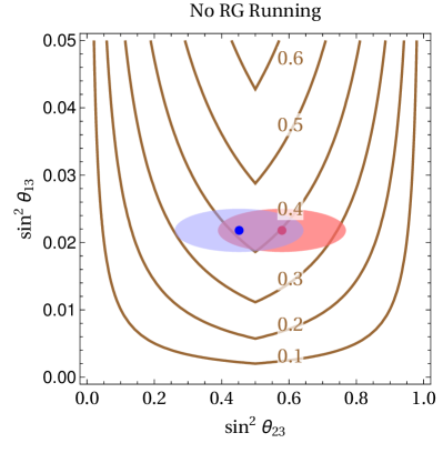
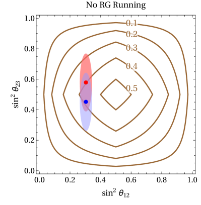
This implies that the probability that a set of mixing angles randomly chosen according to the Haar measure gives worse p𝑝p-values than the experimentally observed ones is 41.1%. We can thus conclude that the data is well consistent with the anarchy hypothesis, in accord with ref. [5]. Figure 1 shows the value of PKSsubscript𝑃KSP_{\text{KS}} as a function of sin2θ12obssuperscript2superscriptsubscript𝜃12obs\sin^{2}\theta_{12}^{\text{obs}} and sin2θ23obssuperscript2superscriptsubscript𝜃23obs\sin^{2}\theta_{23}^{\text{obs}} (left panel) and of sin2θ23obssuperscript2superscriptsubscript𝜃23obs\sin^{2}\theta_{23}^{\text{obs}} and sin2θ13obssuperscript2superscriptsubscript𝜃13obs\sin^{2}\theta_{13}^{\text{obs}} (right panel), with the third mixing angle fixed in both cases (see ref. [5] for similar plots).
Refer to caption Refer to caption
(a) (b)
Figure 1: (a) Contours of equal probability PKSsubscript𝑃KSP_{\text{KS}} (see eq. (7)) in the sin2θ12superscript2subscript𝜃12\sin^{2}\theta_{12}sin2θ23superscript2subscript𝜃23\sin^{2}\theta_{23} plane. The red (blue) ellipses show the favored region from the global fit in ref. [17] at the 3σ3𝜎3\sigma confidence level for inverted (normal) mass ordering. The colored dots indicate the corresponding best fit points. We have fixed the third mixing angle at its best fit value, sin2θ13=0.0218superscript2subscript𝜃130.0218\sin^{2}\theta_{13}=0.0218. (b) Contours of equal probability PKSsubscript𝑃KSP_{\text{KS}} in the sin2θ23superscript2subscript𝜃23\sin^{2}\theta_{23}sin2θ13superscript2subscript𝜃13\sin^{2}\theta_{13} plane, compared to the experimentally allowed regions for both mass orderings (same coloring as in (a)). We have fixed the solar mixing angle at its best fit value, sin2θ12=0.304superscript2subscript𝜃120.304\sin^{2}\theta_{12}=0.304.

In addition to the KS test, we have considered two additional statistical tests, namely the Anderson–Darling and the Cramér–von Mises tests. For our simple case where only one measurement is available and parameters have uniform distributions in the interval [0,1]01[0,1], the test statistic for the Anderson–Darling test is

DAD(x0)1log(1x0)log(x0),subscript𝐷ADsubscript𝑥011subscript𝑥0subscript𝑥0\displaystyle D_{\text{AD}}(x_{0})\equiv-1-\log(1-x_{0})-\log(x_{0})\,, (11)

and the one for the Cramér–von Mises test reads

DCvM(x0)13x0+x02.subscript𝐷CvMsubscript𝑥013subscript𝑥0superscriptsubscript𝑥02\displaystyle D_{\text{CvM}}(x_{0})\equiv\frac{1}{3}-x_{0}+x_{0}^{2}\,. (12)

It is, however, easy to see that the corresponding p𝑝p-values pAD(x0)subscript𝑝ADsubscript𝑥0p_{\text{AD}}(x_{0}) and pCvM(x0)subscript𝑝CvMsubscript𝑥0p_{\text{CvM}}(x_{0}), i.e. the probabilities that a randomly drawn value xsuperscript𝑥x^{\prime} leads to a larger value for the test statistic than the reference value x0subscript𝑥0x_{0}, are identical to the p𝑝p-value for the KS test, eq. 6. Therefore, the Anderson–Darling and Cramer-von Mises tests do not provide any additional insights. In this context, let us also mention ref. [18], which discusses a Bayesian comparison of various anarchical models to models with flavor symmetries, finding consistence with both and a slight preference for the latter. Similar conclusions have been reached also in ref. [9].

Even though the predictions of the neutrino anarchy scenario depend on the ad hoc choice of the right-handed mass scale \mathcal{M}, it is possible to draw non-trivial conclusions on the relations between different neutrino mass eigenvalues. A particularly interesting quantity to consider in this context is the effective Majorana mass measured in neutrinoless double beta decay,

|mee||jUej2mj|.\displaystyle\big{|}m_{ee}\bigr{|}\equiv\Big{|}\sum_{j}U_{ej}^{2}m_{j}\Big{|}\,. (13)

where Uejsubscript𝑈𝑒𝑗U_{ej} are the elements in the first row of the leptonic mixing matrix and mjsubscript𝑚𝑗m_{j} are the light mass eigenvalues. (In this paper, we always assume neutrinos to have Majorana masses, so that neutrinoless double beta decay is in principle possible.) We will therefore also discuss how neutrinoless double beta decay experiments can probe the predictions of anarchy in the future, and how these predictions are affected by renormalization group running.

III Renormalization Group Evolution and Anarchy

Like all Lagrangian parameters in a quantum field theory, the neutrino masses and mixing parameters are subject to renormalization group running. It follows that, when comparing the predicted probability distribution of a parameter to its measured value, we have to be careful to evaluate both at the same renormalization scale. In particular, neutrino oscillation measurements are typically carried out at energy scales of order MeV–GeV, while the flavor structure of a typical seesaw model depends on scales MGUT1016GeVsimilar-tosubscript𝑀GUTsuperscript1016GeVM_{\text{GUT}}\sim 10^{16}\,\mathrm{GeV}. Therefore, we will in the following repeat the analysis of neutrino anarchy, but now carefully taking into account renormalization group effects.

III.1 Type-I Seesaw Model

The first example we will study is the type-I seesaw scenario, which extends the Standard Model by three heavy gauge singlet neutrinos with Majorana masses of 𝒪(1014GeV)𝒪superscript1014GeV\mathcal{O}(10^{14}\,\mathrm{GeV}), which couple to the active SM neutrinos via a Yukawa coupling [19, 20]. The Lagrangian is given by eq. 1.

The renormalization group equations for the type-I seesaw model have been studied in great detail in refs. [21, 22, 23, 24, 25]. To investigate the effect of RG evolution on neutrino anarchy in this model, we have randomly generated 105superscript10510^{5} sets of parameters, defined by the Yukawa matrices Yνsubscript𝑌𝜈Y_{\nu} and the right-handed neutrino mass matrices M𝑀M. We assume these randomly generated matrices to enter the Lagrangian at the high scale MGUT=1016subscript𝑀GUTsuperscript1016M_{\text{GUT}}=10^{16} GeV. As explained in ref. [16], to ensure basis invariance of the probability distributions and statistical independence of different mass matrix elements, the elements of Yναβsuperscriptsubscript𝑌𝜈𝛼𝛽Y_{\nu}^{\alpha\beta} must follow a Gaussian distribution exp[|Yναβ|2/𝒴]proportional-toabsentsuperscriptsuperscriptsubscript𝑌𝜈𝛼𝛽2𝒴\propto\exp[-|Y_{\nu}^{\alpha\beta}|^{2}/\mathcal{Y}]. The diagonal elements Mααsuperscript𝑀𝛼𝛼M^{\alpha\alpha} of the right-handed Majorana mass matrix follow a similar distribution exp[|Mαα|2/]proportional-toabsentsuperscriptsuperscript𝑀𝛼𝛼2\propto\exp[-|M^{\alpha\alpha}|^{2}/\mathcal{M}], while the distribution of the off-diagonal elements Mαβsuperscript𝑀𝛼𝛽M^{\alpha\beta} of M𝑀M is exp[2|Mαβ|2/]proportional-toabsent2superscriptsuperscript𝑀𝛼𝛽2\propto\exp[-2|M^{\alpha\beta}|^{2}/\mathcal{M}]. Here 𝒴𝒴\mathcal{Y} is a dimensionless parameter which we choose to be one, while \mathcal{M} is dimensionful, and we choose =1014superscript1014\mathcal{M}=10^{14} GeV to reproduce the correct order of magnitude for the light neutrino masses. Below we will discuss the impact of different choices for \mathcal{M}.

For the parameters of the standard model at the high scale we have chosen a set of values offered by the REAP package [21]:

Yu(MGUT)subscript𝑌𝑢subscript𝑀GUT\displaystyle Y_{u}(M_{\text{GUT}}) =(5.40391061.56371030.4829),absentmatrix5.4039superscript106missing-subexpressionmissing-subexpressionmissing-subexpression1.5637superscript103missing-subexpressionmissing-subexpressionmissing-subexpression0.4829\displaystyle=\begin{pmatrix}5.4039\cdot 10^{-6}&&\\ &1.5637\cdot 10^{-3}&\\ &&0.4829\end{pmatrix}\,, (14)
Yd(MGUT)subscript𝑌𝑑subscript𝑀GUT\displaystyle Y_{d}(M_{\text{GUT}}) =105×(2.11764.5697+0.0112i2.1367+0.2581i4.56970.0112i22.369825.70970.0019i2.13670.2571i25.7097+0.0019i614.0010),absentsuperscript105matrix2.11764.56970.0112𝑖2.13670.2581𝑖4.56970.0112𝑖22.369825.70970.0019𝑖2.13670.2571𝑖25.70970.0019𝑖614.0010\displaystyle=10^{-5}\times\begin{pmatrix}2.1176&4.5697+0.0112i&2.1367+0.2581i\\ 4.5697-0.0112i&22.3698&25.7097-0.0019i\\ 2.1367-0.2571i&25.7097+0.0019i&614.0010\end{pmatrix}\,,
Ye(MGUT)subscript𝑌𝑒subscript𝑀GUT\displaystyle Y_{e}(M_{\text{GUT}}) =(2.83701060.598810310.1789103).absentmatrix2.8370superscript106missing-subexpressionmissing-subexpressionmissing-subexpression0.5988superscript103missing-subexpressionmissing-subexpressionmissing-subexpression10.1789superscript103\displaystyle=\begin{pmatrix}2.8370\cdot 10^{-6}&&\\ &0.5988\cdot 10^{-3}&\\ &&10.1789\cdot 10^{-3}\end{pmatrix}\,.

Of course the low-scale values of the quark and charged lepton Yukawa matrices depend on the additional field content beyond the SM and on the values of the new parameters introduced. Therefore, we typically cannot reproduce the SM Yukawa couplings exactly, with deviations being of order 10%. Nevertheless, since our interest here is in the running of the neutrino masses and mixing parameters, these small deviations are negligible for our purposes.

We evolve each parameter point down to a lower scale, which we take to be MZ=91.19GeVsubscript𝑀𝑍91.19GeVM_{Z}=91.19\,\mathrm{GeV}. In principle, we should evolve the mixing parameters down to an even lower scale, integrating out SM particles along the way. However, as we will see, the dominant contribution to the running of the mixing parameters arises at scales MZmuch-greater-thanabsentsubscript𝑀𝑍\gg M_{Z} and thus it is justified to stop the RG evolution at MZsubscript𝑀𝑍M_{Z}. The renormalization group equations for the type-I seesaw scenario have been derived in [21], and we follow the exact same procedure. Both at MGUTsubscript𝑀GUTM_{\text{GUT}} and at MZsubscript𝑀𝑍M_{Z}, we extract the values of the physical mixing parameters by diagonalizing the mass matrices and then following appendix A of ref. [14]. In diagonalizing mνsubscript𝑚𝜈m_{\nu}, we have to specify a convention for the ordering of the mass eigenvalues. We always choose them to be in ascending order (case A3 in ref. [15]). Note that for the running of the neutrino masses, decoupling effects cannot be neglected and even the top-quark decoupling may become important [26]. However, since we are mostly interested in the running of the mixing angles and CP phases here, it is justified to neglect decoupling effects. This is especially true for the top and the Higgs because the running of the mixing parameters is negligible at their mass scale (see e.g. fig. 4 below).
Refer to caption
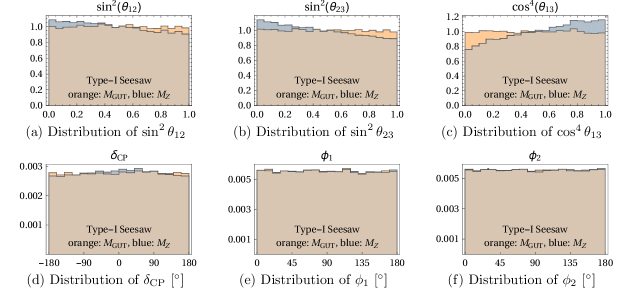
Figure 2: Distributions of the three mixing angles, the Dirac CP phase δCPsubscript𝛿CP\delta_{\text{CP}} and the two Majorana CP phases ϕ1subscriptitalic-ϕ1\phi_{1} and ϕ2subscriptitalic-ϕ2\phi_{2} before and after renormalization group running in the type-I seesaw model. Orange regions correspond to parameters at MGUTsubscript𝑀GUTM_{\text{GUT}}, blue regions to parameters at MZsubscript𝑀𝑍M_{Z}. Note that the physical range for δCPsubscript𝛿CP\delta_{\text{CP}} is [180°,180°)180°180°[-180\degree,180\degree), while the physical ranges for ϕ1subscriptitalic-ϕ1\phi_{1} and ϕ2subscriptitalic-ϕ2\phi_{2} are only [0,180°)0180°[0,180\degree) [15].
Refer to caption
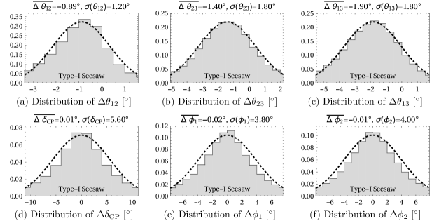
Figure 3: Distributions of the RG-induced shifts in the mixing parameters, Δxx(MZ)x(MGUT)Δ𝑥𝑥subscript𝑀𝑍𝑥subscript𝑀GUT\Delta x\equiv x(M_{Z})-x(M_{\text{GUT}}) in the type-I seesaw model. Also shown are the central values Δx¯¯Δ𝑥\overline{\Delta x} and the widths σ(x)𝜎𝑥\sigma(x) of Gaussian fits to the distributions.

We show our results in fig. 2. In each panel, we compare the distribution of one of the mixing parameters at MGUTsubscript𝑀GUTM_{\text{GUT}} (orange histograms) to the distribution at MZsubscript𝑀𝑍M_{Z} after RG running (blue histograms). By construction, the distributions at MGUTsubscript𝑀GUTM_{\text{GUT}} are flat, while at MZsubscript𝑀𝑍M_{Z}, we observe a small bias towards smaller mixing angles. We show in fig. 3 the distributions of the RG-induced shifts, Δx=x(MZ)x(MGUT)Δ𝑥𝑥subscript𝑀𝑍𝑥subscript𝑀GUT\Delta x=x(M_{Z})-x(M_{\text{GUT}}), where x{θ12,θ13,θ23,δCP,ϕ1,ϕ2}𝑥subscript𝜃12subscript𝜃13subscript𝜃23subscript𝛿CPsubscriptitalic-ϕ1subscriptitalic-ϕ2x\in\{\theta_{12},\theta_{13},\theta_{23},\delta_{\text{CP}},\phi_{1},\phi_{2}\}. We have also fitted each histogram in fig. 3 to a Gaussian distribution

f(x)=12πσ(x)exp[(xx¯)22[σ(x)]2],𝑓𝑥12𝜋𝜎𝑥superscript𝑥¯𝑥22superscriptdelimited-[]𝜎𝑥2\displaystyle f(x)=\frac{1}{\sqrt{2\pi}\sigma(x)}\exp\bigg{[}-\frac{(x-\overline{x})^{2}}{2[\sigma(x)]^{2}}\bigg{]}\,, (15)

and we give the fitted values of x¯¯𝑥\overline{x} and σ(x)𝜎𝑥\sigma(x) in the plots.

Refer to caption
Figure 4: A parameter point of the type-I seesaw model with large running effects in the neutrino mixing angles. The vertical dotted lines show the decoupling thresholds of the heavy singlet neutrinos, M1=2.91013GeVsubscript𝑀12.9superscript1013GeVM_{1}=2.9\cdot 10^{13}\,\mathrm{GeV}, M2=9.21013GeVsubscript𝑀29.2superscript1013GeVM_{2}=9.2\cdot 10^{13}\,\mathrm{GeV} and M3=1.671014GeVsubscript𝑀31.67superscript1014GeVM_{3}=1.67\cdot 10^{14}\,\mathrm{GeV} . Note how RG running ceases after the last heavy neutrino is integrated out. The masses of the active neutrinos at the low scale are m1=0.02eVsubscript𝑚10.02eVm_{1}=0.02\,\mathrm{eV}, m2=0.32eVsubscript𝑚20.32eVm_{2}=0.32\,\mathrm{eV} and m3=0.36eVsubscript𝑚30.36eVm_{3}=0.36\,\mathrm{eV}.

We find a slight preference for the mixing angles to decrease by 1–2 after evolving them from MGUTsubscript𝑀GUTM_{\text{GUT}} to MZsubscript𝑀𝑍M_{Z}: the distributions of ΔθijΔsubscript𝜃𝑖𝑗\Delta\theta_{ij} all peak at small negative values. The distribution of the Dirac CP phase δCPsubscript𝛿CP\delta_{\text{CP}} in fig. 2 (d) shows a slight peak at zero after running, while the distributions of the Majorana phases ϕ1subscriptitalic-ϕ1\phi_{1} and ϕ2subscriptitalic-ϕ2\phi_{2} in fig. 2 (e), (f) are flat both at MGUTsubscript𝑀GUTM_{\text{GUT}} and at MZsubscript𝑀𝑍M_{Z}. These are of course only statements about the average behavior of a large set of random parameter points—individual points can lead to much larger running effects. In particular, for scenarios where at least two neutrino mass eigenvalues are very close to each other, the running of the mixing angles is known to be potentially large [21].

Even for parameter points that exhibit significant RG running, we observe that most of the running happens at scales above the masses of the heavy singlet neutrinos. Figure 4 shows an example where the mixing angles exhibit large RG running. We observe that the running gradually diminishes as the heavy singlet neutrinos are integrated out and completely ceases below the mass of the lightest of them. This observation allows us to draw conclusions on the impact of the right-handed neutrino mass scale \mathcal{M} on the RG evolution: For \mathcal{M} larger (smaller) than our choice =1014superscript1014\mathcal{M}=10^{14} GeV, the singlet neutrinos are typically heavier (lighter), so the running ceases sooner (later), and the overall shift in the parameters will be smaller (larger). We explicitly checked this behavior numerically.

The fact that the mixing angles run preferentially downwards can be understood in the following way. First, recall that the leptonic mixing matrix depends on the matrix Vνsubscript𝑉𝜈V_{\nu} that diagonalizes mνsubscript𝑚𝜈m_{\nu} and on the matrix Vesubscript𝑉𝑒V_{e} that diagonalizes YeYesuperscriptsubscript𝑌𝑒subscript𝑌𝑒Y_{e}^{\dagger}Y_{e} according to VeYeYeVe=Dsubscript𝑉𝑒superscriptsubscript𝑌𝑒subscript𝑌𝑒superscriptsubscript𝑉𝑒𝐷V_{e}Y_{e}^{\dagger}Y_{e}V_{e}^{\dagger}=D, where D𝐷D is diagonal. The flavor non-trivial terms in the β𝛽\beta functions for the mass and Yukawa matrices (see appendix A) are dominated by the 𝒪(1)𝒪1\mathcal{O}(1) terms containing Yνsubscript𝑌𝜈Y_{\nu}. The subdominant terms involving Yesubscript𝑌𝑒Y_{e} are negligible. Since Yνsubscript𝑌𝜈Y_{\nu} is randomly chosen, it cannot lead to a preference for one sign over the other in the β𝛽\beta function. Thus, the only possible source of such a preference can come from the initial conditions for Yesubscript𝑌𝑒Y_{e}. The β𝛽\beta function for Yesubscript𝑌𝑒Y_{e} reads

16π2βYe=32Ye(YνYν)+.16superscript𝜋2subscript𝛽subscript𝑌𝑒32subscript𝑌𝑒superscriptsubscript𝑌𝜈subscript𝑌𝜈\displaystyle 16\pi^{2}\beta_{Y_{e}}=-\frac{3}{2}Y_{e}\big{(}Y_{\nu}^{\dagger}Y_{\nu}\big{)}+\dots\,. (16)

where the dots indicate the subdominant and flavor-diagonal terms. The initial condition Ye(MGUT)subscript𝑌𝑒subscript𝑀GUTY_{e}(M_{\text{GUT}}) for Yesubscript𝑌𝑒Y_{e} is a diagonal matrix (see eq. 14), with its strongly hierarchical eigenvalues sorted in ascending order. The structure of eq. 16 shows that after RG running, the elements in the k𝑘k-th row of Yesubscript𝑌𝑒Y_{e} will change by an amount proportional to the (kk)𝑘𝑘(kk) elements of Ye(MGUT)subscript𝑌𝑒subscript𝑀GUTY_{e}(M_{\text{GUT}}). To proceed, it is easiest to consider a two flavor system for illustrative purposes. In this case, using the hierarchy of the elements of Yesubscript𝑌𝑒Y_{e} after running, one can show that the mixing angle parameterizing Vesubscript𝑉𝑒V_{e} is positive. Since UPMNS=VeVνsubscript𝑈PMNSsuperscriptsubscript𝑉𝑒subscript𝑉𝜈U_{\text{PMNS}}=V_{e}^{\dagger}V_{\nu}, and since the mixing angle describing Vνsubscript𝑉𝜈V_{\nu} is random in [π,π]𝜋𝜋[-\pi,\pi], the mixing angle describing UPMNSsubscript𝑈PMNSU_{\text{PMNS}} is then preferentially negative. In models where the dominant term in (16) comes with a different sign, the preferred direction of the running would be reversed. One example of such model is a type-II seesaw model [27].

To study how RG running affects the compatibility of neutrino anarchy with the observed mixing parameters, we use again the Kolmogorov–Smirnov test. Note that the multidimensional KS test described in section II is only meaningful if the parameters in the integral eq. 7 are statistically independent and follow a flat distribution. We have checked that, even after RG running, the parameters sin2θ12superscript2subscript𝜃12\sin^{2}\theta_{12}, sin2θ23superscript2subscript𝜃23\sin^{2}\theta_{23} and cos4θ13superscript4subscript𝜃13\cos^{4}\theta_{13} are still nearly uncorrelated. For instance, the modulus of Pearson’s correlation coefficient, |xy/(xy)|delimited-⟨⟩𝑥𝑦delimited-⟨⟩𝑥delimited-⟨⟩𝑦\big{|}\left\langle x\cdot y\right\rangle/(\left\langle x\right\rangle\left\langle y\right\rangle)\big{|}, is 0.02less-than-or-similar-toabsent0.02\lesssim 0.02 for all combinations of x,y=sin2θ12,sin2θ23,cos4θ13formulae-sequence𝑥𝑦superscript2subscript𝜃12superscript2subscript𝜃23superscript4subscript𝜃13x,\,y=\sin^{2}\theta_{12},\,\sin^{2}\theta_{23},\,\cos^{4}\theta_{13}. To obtain flat distributions, we define new parameters sin2θ12superscript2superscriptsubscript𝜃12\sin^{2}\theta_{12}^{\prime}, sin2θ23superscript2superscriptsubscript𝜃23\sin^{2}\theta_{23}^{\prime} and cos4θ13superscript4superscriptsubscript𝜃13\cos^{4}\theta_{13}^{\prime} in the following way: we fit each of the distributions in fig. 2 (a), (b), (c) by a cubic polynomial f(x)𝑓𝑥f(x), where x=sin2θ12𝑥superscript2subscript𝜃12x=\sin^{2}\theta_{12}, sin2θ23superscript2subscript𝜃23\sin^{2}\theta_{23}, cos4θ13superscript4subscript𝜃13\cos^{4}\theta_{13}. We normalize f(x)𝑓𝑥f(x) such that its integral over the physical range of x𝑥x is 1. We then define x(x)0x𝑑x~f(x~)superscript𝑥𝑥superscriptsubscript0𝑥differential-d~𝑥𝑓~𝑥x^{\prime}(x)\equiv\int_{0}^{x}\!d\tilde{x}\,f(\tilde{x}). Replacing the unprimed variables x𝑥x in eq. 7 by the primed ones x(x)superscript𝑥𝑥x^{\prime}(x), the KS test can now be applied in a meaningful way.
Refer to caption Refer to caption
(a) (b)
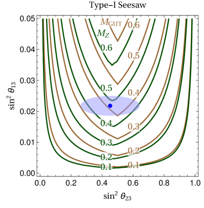
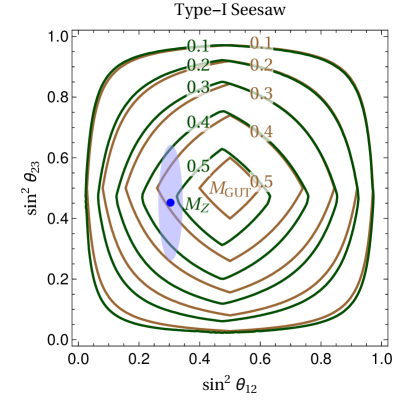
Figure 5: (a) Contours of equal probability PKS,NHsubscript𝑃KS,NHP_{\text{KS,NH}} (see eqs. 7 and 9) in the sin2θ12superscript2subscript𝜃12\sin^{2}\theta_{12}sin2θ23superscript2subscript𝜃23\sin^{2}\theta_{23} plane with RG effects included (dark green) and without RG effects (brown, see fig. 1 (a)) for the type-I seesaw model. We consider only parameter points with a normal mass ordering (see text for details). The blue ellipse indicates the normal ordering favored region from the global fit in ref. [17] at the 3σ3𝜎3\sigma confidence level, and the blue dot is the corresponding best fit point. We have fixed the third mixing angle at its best fit value, sin2θ13=0.0218superscript2subscript𝜃130.0218\sin^{2}\theta_{13}=0.0218. With RG effects included, the likelihood of the data with respect to anarchy increases from 41.1% to 47.7%. (b) Contours of equal probability PKS,NHsubscript𝑃KS,NHP_{\text{KS,NH}} in the sin2θ23superscript2subscript𝜃23\sin^{2}\theta_{23}sin2θ13superscript2subscript𝜃13\sin^{2}\theta_{13} plane with and without RG effects included (same coloring as in (a)). We have fixed the solar mixing angle at its best fit value, sin2θ12=0.304superscript2subscript𝜃120.304\sin^{2}\theta_{12}=0.304.

A further subtlety arises because the RG evolution is different for parameter points with a normal mass ordering and parameter points with an inverted mass ordering. We therefore separate our randomly generated points according to the predicted mass ordering and compute PKS,NHsubscript𝑃KS,NHP_{\text{KS,NH}} (PKS,IHsubscript𝑃KS,IHP_{\text{KS,IH}}) in eq. 9 using only points with normal (inverted) ordering. We find that the probability P~KSsubscript~𝑃KS\tilde{P}_{\text{KS}} of the observed parameter values, given the anarchy hypothesis, increases by 7%similar-toabsentpercent7\sim 7\% from 41.1% to 47.7% due to RG effects. Note that, as before, P~KSsubscript~𝑃KS\tilde{P}_{\text{KS}} is entirely dominated by parameter points with a normal mass ordering because the probability of obtaining an inverted ordering from anarchy is only at the 5% level. We show in fig. 5 the contours of equal Kolmogorov–Smirnov probability PKS,NHsubscript𝑃KS,NHP_{\text{KS,NH}} for parameter points with normal mass ordering before and after running.

Finally, we also comment on the running of the neutrino mass parameters, which we find to be substantial. Parameterizing their approximate evolution as dm/dlogμ=γm𝑑𝑚𝑑𝜇𝛾𝑚dm/d\log\mu=-\gamma m, we find for the anomalous dimension of the three light mass eigenvalues an average value of γ0.027similar-to-or-equals𝛾0.027\gamma\simeq-0.027. This implies that the light neutrino masses run down by about 60% between MGUTsubscript𝑀GUTM_{\text{GUT}} and MZsubscript𝑀𝑍M_{Z}.

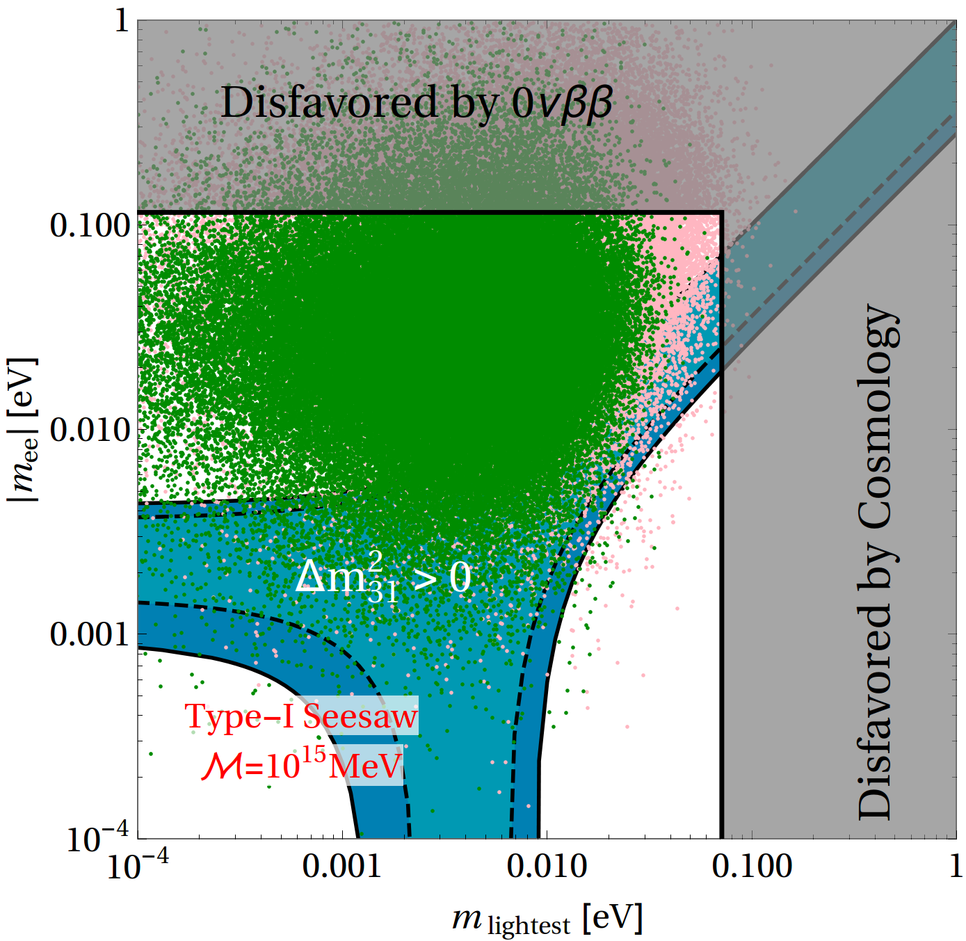
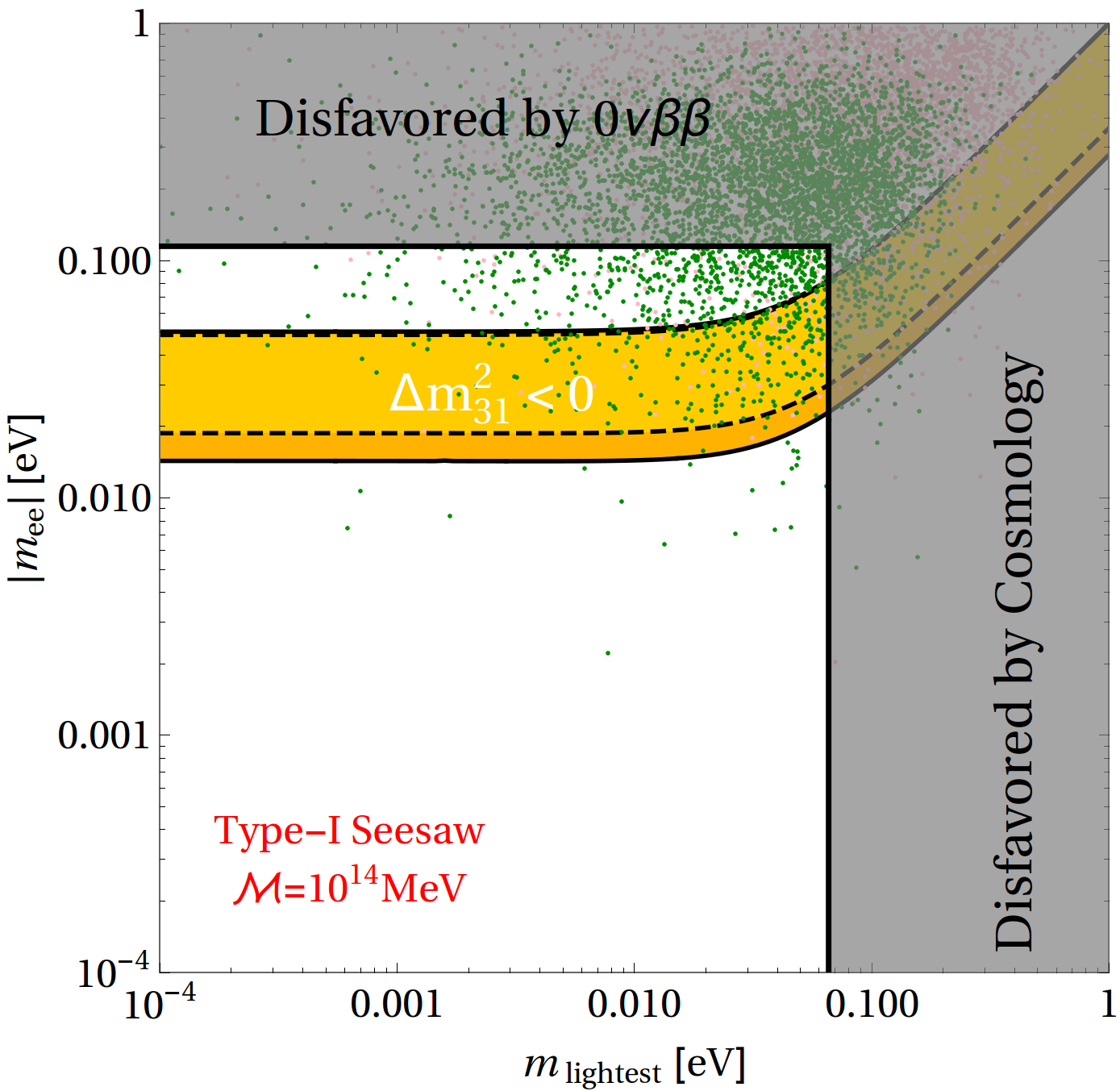
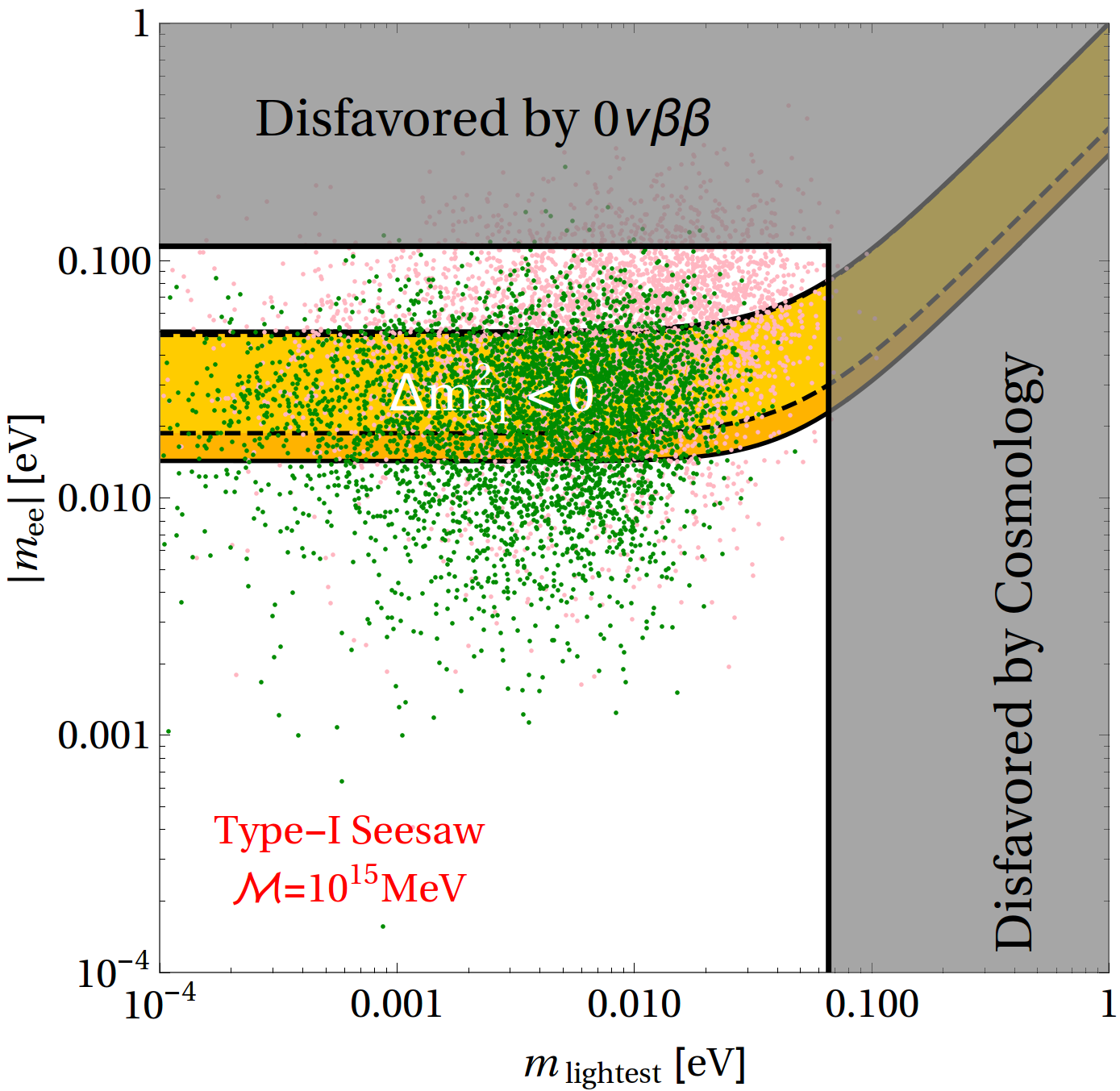
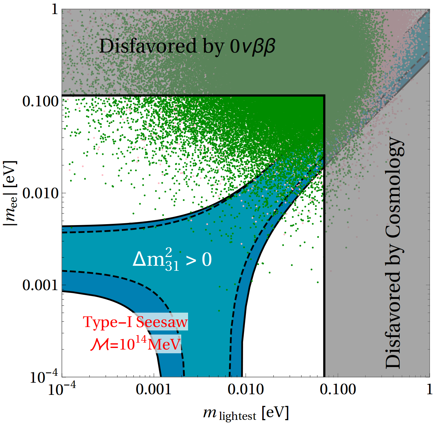
We investigate in fig. 6 what neutrino anarchy with and without RG running predicts for the outcome of future neutrinoless double beta (0ν2β0𝜈2𝛽0\nu 2\beta) decay experiments. Of course, since the scale choice \mathcal{M} for the right-handed neutrinos is an input parameter even in the anarchy scenario, the absolute scale of mlightestsubscript𝑚lightestm_{\text{lightest}} and meesubscript𝑚𝑒𝑒m_{ee} can be chosen at will. In fact, the left and right panels in fig. 6 represent two different choices for \mathcal{M}. Nonetheless, we can draw several important conclusions from fig. 6. First, we see again that anarchy favors the normal mass ordering: there are much fewer points in panels (c) and (d) than in panels (a) and (b). In other words, if a future 0ν2β0𝜈2𝛽0\nu 2\beta search finds a result compatible only with an inverted mass ordering, this would disfavor anarchy. Second, we see that scenarios with relatively large meesubscript𝑚𝑒𝑒m_{ee} but very small mlightestsubscript𝑚lightestm_{\text{lightest}}, such as the leftmost part of the inverted hierarchy band, are disfavored, as are scenarios with very small meesubscript𝑚𝑒𝑒m_{ee} but sizeable mlightestsubscript𝑚lightestm_{\text{lightest}}, in particular the funnel region in the normal hierarchy case. Finally, also a quasi-degenerate mass spectrum is disfavored by the anarchy hypothesis. If a combination of 0ν2β0𝜈2𝛽0\nu 2\beta experiments, cosmology and direct neutrino mass measurements should point to one of these disfavored regions in the future, the anarchy hypothesis would come under pressure.
Refer to caption Refer to caption
(a) (b)
Refer to caption Refer to caption
(c) (d)
Figure 6: Colored dots: predictions for the effective mass |mee|subscript𝑚𝑒𝑒|m_{ee}| measured in neutrinoless double beta decay from the neutrino anarchy scenario in the type-I seesaw model. The mass scale of the right-handed neutrinos was set to =1014GeVsuperscript1014GeV\mathcal{M}=10^{14}\ \text{GeV} in the left panels, and to =1015GeVsuperscript1015GeV\mathcal{M}=10^{15}\ \text{GeV} in the right panels. Among the randomly generated parameter points, we distinguish those resulting in a normal neutrino mass ordering (upper panels) and those resulting in an inverted ordering (lower panels). Pink points show the distributions at MGUTsubscript𝑀GUTM_{\text{GUT}}, while green points show the shifted distributions after renormalization group evolution to MZsubscript𝑀𝑍M_{Z}. The colored bands show the allowed regions in the mlightestsubscript𝑚lightestm_{\text{lightest}}|mee|subscript𝑚𝑒𝑒|m_{ee}| plane from the global experimental data on the neutrino mass squared differences and mixing angles. Dashed lines correspond to varying only the unknown phases in UPMNSsubscript𝑈PMNSU_{\text{PMNS}}, while solid lines also include the uncertainties in the mixing angles. Note that, to be true to the spirit of anarchy, we do not impose any constraints on our randomly generated points, therefore a sizeable portion of them fall into regions already excluded by experiment. Gray regions are exclusion limits from cosmology [28] and from experimental searches for neutrinoless double beta decay [29, 30, 31].

III.2 Inverse Seesaw Model

As a second example, we consider the inverse seesaw scenario [32, 33], in which the SM Lagrangian is extended by

inverse seesaw(Yν)αβL¯αH~NRβMDαβS¯α(NRβ)c12msαβS¯α(Sβ)c+h.c.,formulae-sequencesuperscriptsuperscriptsubscript𝑌𝜈𝛼𝛽superscript¯𝐿𝛼~𝐻superscriptsubscript𝑁𝑅𝛽superscriptsubscript𝑀𝐷𝛼𝛽superscript¯𝑆𝛼superscriptsuperscriptsubscript𝑁𝑅𝛽𝑐12superscriptsubscript𝑚𝑠𝛼𝛽superscript¯𝑆𝛼superscriptsuperscript𝑆𝛽𝑐subscriptinverse seesaw𝑐\displaystyle\mathcal{L}_{\text{inverse seesaw}}\supset-(Y_{\nu}^{\dagger})^{\alpha\beta}\bar{L}^{\alpha}\tilde{H}N_{R}^{\beta}-M_{D}^{\alpha\beta}\bar{S}^{\alpha}(N_{R}^{\beta})^{c}-\frac{1}{2}m_{s}^{\alpha\beta}\bar{S}^{\alpha}(S^{\beta})^{c}+h.c.\,, (17)

where two types of new gauge singlet Weyl fermions are introduced: nNsubscript𝑛𝑁n_{N} generations of NRsubscript𝑁𝑅N_{R} fields, which participate directly in the Yukawa couplings, and nSsubscript𝑛𝑆n_{S} generations of S𝑆S fields. Possible completions of the model that explain this structure for the Lagrangian are given in [34, 35, 36, 37]. After electroweak symmetry breaking, the neutrino mass term becomes:

m,inverse seesaw(νLc¯,N¯R,S¯)(0YνTv/20Yνv/20MDT0MDms)(νLNRcSc).¯superscriptsubscript𝜈𝐿𝑐subscript¯𝑁𝑅¯𝑆matrix0subscriptsuperscript𝑌𝑇𝜈𝑣20subscript𝑌𝜈𝑣20subscriptsuperscript𝑀𝑇𝐷0subscript𝑀𝐷subscript𝑚𝑠matrixsubscript𝜈𝐿superscriptsubscript𝑁𝑅𝑐superscript𝑆𝑐subscript𝑚inverse seesaw\displaystyle\mathcal{L}_{m,\text{inverse seesaw}}\supset-\big{(}\overline{\nu_{L}^{c}},\bar{N}_{R},\bar{S}\big{)}\begin{pmatrix}0&Y^{T}_{\nu}v/\sqrt{2}&0\\ Y_{\nu}v/\sqrt{2}&0&M^{T}_{D}\\ 0&M_{D}&m_{s}\end{pmatrix}\begin{pmatrix}\nu_{L}\\ N_{R}^{c}\\ S^{c}\end{pmatrix}\,. (18)

For the effective Majorana mass matrix of the light active neutrinos we then obtain:

mνv22YνTMD1msMD1Yν.similar-to-or-equalssubscript𝑚𝜈superscript𝑣22superscriptsubscript𝑌𝜈𝑇superscriptsubscript𝑀𝐷1subscript𝑚𝑠superscriptsubscript𝑀𝐷1subscript𝑌𝜈\displaystyle m_{\nu}\simeq\frac{v^{2}}{2}Y_{\nu}^{T}M_{D}^{-1}m_{s}M_{D}^{-1}Y_{\nu}\,. (19)

The correct neutrino mass eigenvalues 𝒪(eV)less-than-or-similar-toabsent𝒪eV\lesssim\mathcal{O}(\text{eV}) are obtained for MD𝒪(TeV)similar-tosubscript𝑀𝐷𝒪TeVM_{D}\sim\mathcal{O}(\text{TeV}), ms𝒪(keV)similar-tosubscript𝑚𝑠𝒪keVm_{s}\sim\mathcal{O}(\text{keV}). The model has the additional virtue that, if the number of generations of S𝑆S is larger than the number of generations of NRsubscript𝑁𝑅N_{R}, 𝒪(keV)𝒪keV\mathcal{O}(\text{keV}) sterile mass eigenstates are obtained [38], which could act as the dark matter in the Universe. (If also NRsubscript𝑁𝑅N_{R} has a Majorana mass term, the condition nS>nNsubscript𝑛𝑆subscript𝑛𝑁n_{S}>n_{N} can be avoided, see e.g. ref. [39].) The RG equations for the inverse seesaw model are given in appendix A. They agree with the ones given in [40].

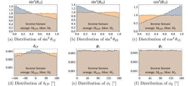
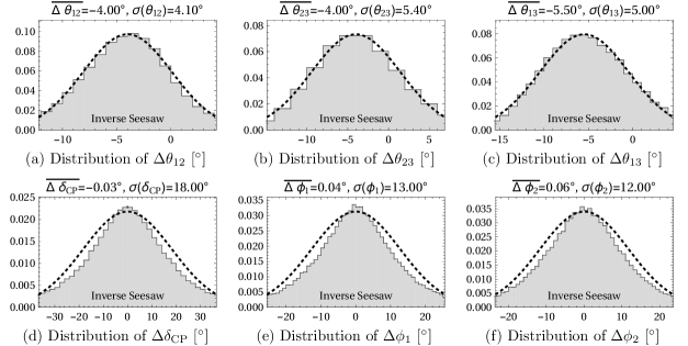
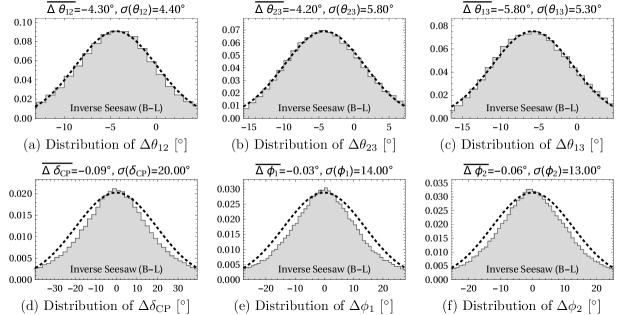
Carrying out an RG analysis on a random sample of 105superscript10510^{5} mass matrices of the form of eq. 18, defined at MGUTsubscript𝑀GUTM_{\text{GUT}} and evolved down to MZsubscript𝑀𝑍M_{Z}, we obtain the results shown in figs. 7 and 8. The shifts in the mixing angles show the same characteristics as in the type-I seesaw model discussed in the previous section. In particular, mixing angles are preferentially shifted to smaller values, and δCPsubscript𝛿CP\delta_{\text{CP}} is preferentially close to zero. The average magnitude of the shifts is, however, larger than in the type-I seesaw case: of order 4°4°4\degree for θ12subscript𝜃12\theta_{12} and θ23subscript𝜃23\theta_{23}, and of order 5.5°5.5°5.5\degree for θ13subscript𝜃13\theta_{13}. Also the widths of the distributions in fig. 8 are several times larger than they were for the type-I seesaw model (see fig. 3). The average anomalous dimension describing the running of the light neutrino masses is -0.037 in the inverse seesaw scenario, corresponding to a 70% decrease of the mass eigenvalues between MGUTsubscript𝑀GUTM_{\text{GUT}} and MZsubscript𝑀𝑍M_{Z}.

Refer to caption
Figure 7: Distributions of the mixing angles and physical CP phases before and after renormalization group running in the inverse seesaw model. The orange regions correspond to the parameters at MGUTsubscript𝑀GUTM_{\text{GUT}}, the blue regions to the parameters at MZsubscript𝑀𝑍M_{Z}. As for the type-I seesaw model, the distributions of the Majorana CP phases are unaffected by RG evolution. For the mixing angles and the Dirac CP phase, the running is much stronger than in the type-I seesaw case.
Refer to caption
Figure 8: Shift in the mixing angles and the CP phases during RG evolution form MGUTsubscript𝑀GUTM_{\text{GUT}} to MZsubscript𝑀𝑍M_{Z} in the inverse seesaw model, obtained from 105superscript10510^{5} randomly generated mass matrices. We use the notation Δxx(MZ)x(MGUT)Δ𝑥𝑥subscript𝑀𝑍𝑥subscript𝑀GUT\Delta x\equiv x(M_{Z})-x(M_{\text{GUT}}), where x𝑥x stands for any of the mixing angles or complex phases. Also shown are Gaussian fits with central values Δx¯¯Δ𝑥\overline{\Delta x} and widths σ(Δx)𝜎Δ𝑥\sigma(\Delta x).
Refer to caption Refer to caption
(a) (b)
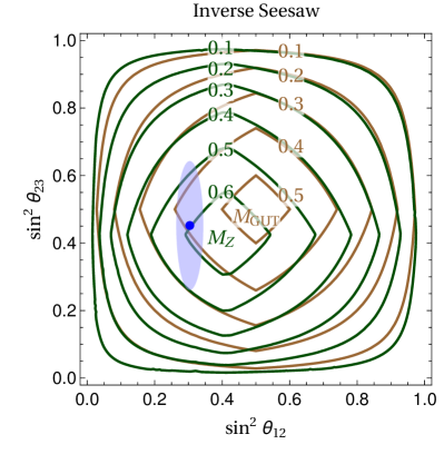
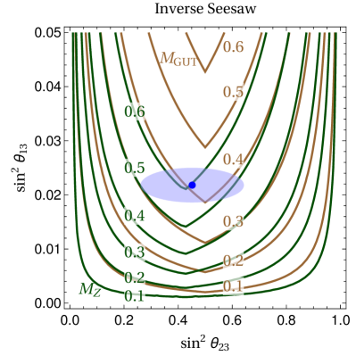
Figure 9: (a) Contours of equal probability PKS,NHsubscript𝑃KS,NHP_{\text{KS,NH}} (see eqs. 7 and 9) in the sin2θ12superscript2subscript𝜃12\sin^{2}\theta_{12}sin2θ23superscript2subscript𝜃23\sin^{2}\theta_{23} plane with RG effects included (dark green) and without RG effects (brown,see fig. 1) for the inverse seesaw model. We consider only parameter points with a normal mass ordering (see text in section III.1 for details). The blue ellipses denote the favored parameter region from the global fit in ref. [17] at the 3σ3𝜎3\sigma confidence level, and the blue dot is the corresponding best fit point. We have fixed the third mixing angle at its best fit value, sin2θ13=0.0218superscript2subscript𝜃130.0218\sin^{2}\theta_{13}=0.0218. With RG effects included, the likelihood of the data with respect to the anarchy hypothesis increases from 41.1% to 59.3%. (b) Contours of equal probability PKS,NHsubscript𝑃KS,NHP_{\text{KS,NH}} in the sin2θ23superscript2subscript𝜃23\sin^{2}\theta_{23}sin2θ13superscript2subscript𝜃13\sin^{2}\theta_{13} plane with and without RG effects included (same coloring as in (a)). The solar mixing angle is fixed at its best fit value, sin2θ12=0.304superscript2subscript𝜃120.304\sin^{2}\theta_{12}=0.304.

To see how RG effects influence the consistency of the neutrino oscillation data with the predictions of anarchy, we compare in fig. 9 the equiprobability contours with and without RG running in the inverse seesaw model. To produce this plot, we follow the same procedure as for the type-I seesaw model (see section III.1). We exploit again the fact that the mixing parameters are still nearly uncorrelated after RG evolution, even though the absolute values of the correlation coefficients are now somewhat larger, 0.07similar-toabsent0.07\sim 0.07 now. We find that RG effects change the compatibility of the anarchy hypothesis with the data substantially: P~KSsubscript~𝑃KS\tilde{P}_{\text{KS}} increases from 41.1% without RG effects to 59.3% with RG running included.

III.3 Inverse Seesaw model with gauged 𝑼(𝟏)𝑩𝑳𝑼subscript1𝑩𝑳\bm{U(1)_{B-L}}

field Spin U(1)BL𝑈subscript1𝐵𝐿U(1)_{B-L} charge QBLsubscript𝑄𝐵𝐿Q_{B-L}
χ𝜒\chi 0 11-1
NRsubscript𝑁𝑅N_{R} 1212\frac{1}{2} 11-1
S𝑆S 1212\frac{1}{2} +22+2
Ssuperscript𝑆S^{\prime} 1212\frac{1}{2} 22-2
Zμsuperscriptsubscript𝑍𝜇Z_{\mu}^{\prime} 1 00
Table 1: The new field content of the inverse seesaw model with gauged U(1)BL𝑈subscript1𝐵𝐿U(1)_{B-L}. All listed fields are SM singlets. As usual, standard model leptons have BL𝐵𝐿B-L charge 11-1, while quarks have BL𝐵𝐿B-L charges of 1/3131/3.

As an example for a specific realization of the inverse seesaw mechanism, we consider an extension of the SM where the difference of baryon number and lepton number, BL𝐵𝐿B-L, is gauged [41]. The corresponding gauge boson Zsuperscript𝑍Z^{\prime} is assumed to have a mass of order 100TeV100TeV100\ \text{TeV} generated by the vacuum expectation value (vev) of a new scalar χ𝜒\chi with quantum numbers (1,1,0,1)1101(1,1,0,-1) under SU(3)c×SU(2)L×U(1)Y×U(1)BL𝑆𝑈subscript3𝑐𝑆𝑈subscript2𝐿𝑈subscript1𝑌𝑈subscript1𝐵𝐿SU(3)_{c}\times SU(2)_{L}\times U(1)_{Y}\times U(1)_{B-L}. The fermionic field content of the model is the same as in the phenomenological inverse seesaw model discussed in section III.2 (nNsubscript𝑛𝑁n_{N} singlets NRsubscript𝑁𝑅N_{R}, nSsubscript𝑛𝑆n_{S} singlets S𝑆S), but the fermions now carry BL𝐵𝐿B-L charge: the NRsubscript𝑁𝑅N_{R} have BL𝐵𝐿B-L charge QBL=1subscript𝑄𝐵𝐿1Q_{B-L}=-1, while the S𝑆S have QBL=+2subscript𝑄𝐵𝐿2Q_{B-L}=+2. To ensure anomaly cancellation, it is necessary to supplement the model by nSsubscript𝑛𝑆n_{S} extra Weyl fermions Ssuperscript𝑆S^{\prime} with BL𝐵𝐿B-L charge 22-2.111The cancellation of the triangular gauge anomaly requires that ψL(QBLψL)3=ψR(QBLψR)3subscriptsubscript𝜓𝐿superscriptsubscriptsuperscript𝑄subscript𝜓𝐿𝐵𝐿3subscriptsubscript𝜓𝑅superscriptsubscriptsuperscript𝑄subscript𝜓𝑅𝐵𝐿3\sum_{\psi_{L}}(Q^{\psi_{L}}_{B-L})^{3}=\sum_{\psi_{R}}(Q^{\psi_{R}}_{B-L})^{3}, where ψLsubscript𝜓𝐿\psi_{L} and ψRsubscript𝜓𝑅\psi_{R} represent left-handed and right-handed fields, respectively. For simplicity, we assume that couplings of Ssuperscript𝑆S^{\prime} to other fields (except the U(1)BL𝑈subscript1𝐵𝐿U(1)_{B-L} gauge boson) are forbidden by a new discrete symmetry. We will here remain agnostic with regard to the details of this symmetry and simply ignore Ssuperscript𝑆S^{\prime} in our subsequent discussion. The quantum numbers of the new particles in the inverse seesaw model with gauged BL𝐵𝐿B-L are summarized in table 1.

The Lagrangian reads [41]

14ZμνZμν+ψ=NR,S,Siψ¯ψ+(Dμχ)(Dμχ)[(Yν)αβL¯LαH~NRβ+λSαβS¯αχ(NRβ)c+h.c.]+μ2χχ+λ2(χχ)(HH)+λ3(χχ)2+1Λ3Sc¯χ4S,\mathcal{L}\supset-\frac{1}{4}Z^{\prime}_{\mu\nu}Z^{\prime\mu\nu}+\!\!\sum_{\psi=N_{R},S,S^{\prime}}\!\!\!i\,\bar{\psi}\not{D}\psi+(D_{\mu}\chi)(D^{\mu}\chi)^{\dagger}-\big{[}(Y_{\nu}^{\dagger})^{\alpha\beta}\bar{L}_{L}^{\alpha}\tilde{H}\,N_{R}^{\beta}+\lambda_{S}^{\alpha\beta}\,\bar{S}^{\alpha}\chi^{\dagger}(N_{R}^{\beta})^{c}+h.c.\big{]}\\ +\mu_{2}\,\chi^{\dagger}\chi+\lambda_{2}\,(\chi^{\dagger}\chi)(H^{\dagger}H)+\lambda_{3}\ (\chi^{\dagger}\chi)^{2}+\frac{1}{\Lambda^{3}}\overline{S^{c}}\chi^{4}S\,, (20)

where Dμ=μigBLQBLZμsubscript𝐷𝜇subscript𝜇𝑖subscript𝑔𝐵𝐿subscript𝑄𝐵𝐿subscriptsuperscript𝑍𝜇D_{\mu}=\partial_{\mu}-ig_{B-L}Q_{B-L}Z^{\prime}_{\mu} is the covariant derivative. Note that the last term in the second row is dimension 7 and is therefore suppressed by three powers of a cutoff scale ΛΛ\Lambda.222A realization of this term in a renormalizable model requires additional fields. As a proof of principle, we could add a Majorana fermion NRsuperscriptsubscript𝑁𝑅N_{R}^{\prime} and a real scalar ρ𝜌\rho, both of which are total singlets under the SM gauge group and under U(1)BL𝑈subscript1𝐵𝐿U(1)_{B-L}, plus a complex scalar η𝜂\eta with BL𝐵𝐿B-L charge 22-2. If NRsuperscriptsubscript𝑁𝑅N_{R}^{\prime}, ρ𝜌\rho and η𝜂\eta are charged under a new 2subscript2\mathbb{Z}_{2} symmetry under which all other fields are even, the operator Sc¯χ4S/Λ3¯superscript𝑆𝑐superscript𝜒4𝑆superscriptΛ3\overline{S^{c}}\chi^{4}S/\Lambda^{3} is generated through the following diagram:[Uncaptioned image] We have not written down other higher-dimensional operators here since they are not relevant to the phenomenology we are interested in.

As the vev of the new scalar χ𝜒\chi breaks the U(1)BL𝑈subscript1𝐵𝐿U(1)_{B-L} symmetry spontaneously, it endows the BL𝐵𝐿B-L gauge boson with a mass MZ=2gBLχsubscript𝑀superscript𝑍2subscript𝑔𝐵𝐿delimited-⟨⟩𝜒M_{Z^{\prime}}=\sqrt{2}g_{B-L}\left\langle\chi\right\rangle. Moreover, it generates a Dirac-type mass mixing term of the form (MD)αβS¯α(NRβ)csuperscriptsubscript𝑀𝐷𝛼𝛽superscript¯𝑆𝛼superscriptsuperscriptsubscript𝑁𝑅𝛽𝑐(M_{D})^{\alpha\beta}\bar{S}^{\alpha}(N_{R}^{\beta})^{c} with MD=λSχsubscript𝑀𝐷subscript𝜆𝑆delimited-⟨⟩superscript𝜒M_{D}=\lambda_{S}\left\langle\chi^{\dagger}\right\rangle, and a Majorana mass term msSc¯Ssubscript𝑚𝑠¯superscript𝑆𝑐𝑆m_{s}\overline{S^{c}}S with ms=χ4/Λ3subscript𝑚𝑠superscriptdelimited-⟨⟩𝜒4superscriptΛ3m_{s}=\left\langle\chi\right\rangle^{4}/\Lambda^{3}. Note that, in the unbroken phase of U(1)BL𝑈subscript1𝐵𝐿U(1)_{B-L} a Majorana mass term for S𝑆S is forbidden due to its nonzero BL𝐵𝐿B-L charge. After U(1)BL𝑈subscript1𝐵𝐿U(1)_{B-L}-breaking and electroweak symmetry breaking, the neutral components of the SM Higgs doublet H𝐻H and the new scalar χ𝜒\chi mix to form two CP𝐶𝑃CP even scalars [42].

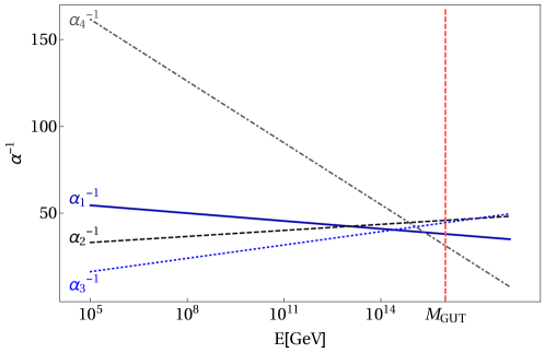
Since our main goal in this section is only to explore whether a UV completion of the inverse seesaw model leads to qualitatively different RG effects, we make several simplifying assumptions in our RG analysis. First, to avoid having to deal with the multitude of different effective theories that can arise depending on where BL𝐵𝐿B-L is broken relative to the masses of the heavy 𝒪(TeV)𝒪TeV\mathcal{O}(\text{TeV}) neutrinos, we always fix the U(1)BL𝑈subscript1𝐵𝐿U(1)_{B-L} breaking scale at fBL=100subscript𝑓𝐵𝐿100f_{B-L}=100 TeV, well above the heavy neutrino masses. Moreover, we assume for simplicity that the BL𝐵𝐿B-L breaking scale fBLsubscript𝑓𝐵𝐿f_{B-L}, the vev χdelimited-⟨⟩𝜒\left\langle\chi\right\rangle, and the mass mχsubscript𝑚𝜒m_{\chi} of χ𝜒\chi are identical, so that we do not need to consider running between these scales. We choose the numerical value of gBLsubscript𝑔𝐵𝐿g_{B-L} such that it unifies to the extent possible at the GUT scale with the SM gauge couplings, see fig. 10. We find that a reasonable choice is gBL=0.58subscript𝑔𝐵𝐿0.58g_{B-L}=0.58 at the GUT scale. By demanding that the running Zsuperscript𝑍Z^{\prime} mass parameter MZ(μ)2gBL(μ)χsubscript𝑀superscript𝑍𝜇2subscript𝑔𝐵𝐿𝜇delimited-⟨⟩𝜒M_{Z^{\prime}}(\mu)\equiv\sqrt{2}g_{B-L}(\mu)\left\langle\chi\right\rangle equals the scale μ𝜇\mu, we find the threshold mass MZ39TeVsubscript𝑀superscript𝑍39TeVM_{Z^{\prime}}\approx 39\leavevmode\nobreak\ \text{TeV}. Since this is sufficiently close to fBL=100TeVsubscript𝑓𝐵𝐿100TeVf_{B-L}=100\leavevmode\nobreak\ \,\mathrm{TeV} on a log scale, we integrate out χ𝜒\chi and Zsuperscript𝑍Z^{\prime} simultaneously. As a further simplification, we ignore renormalization group effects on the quadratic terms in the scalar potential, and consequently the scale dependence of the scalar vevs. Since the scalar quartic couplings do not affect the flavor structure, their only influence on the neutrino mixing parameter can be indirect, by changing the various mass scales of the theory. Finally, we neglect kinetic mixing between the Zsuperscript𝑍Z^{\prime} and the standard model hypercharge gauge boson B𝐵B, which would be allowed by the symmetries. Kinetic mixing is in general absent at the grand unification scale, where we assume that U(1)BL𝑈subscript1𝐵𝐿U(1)_{B-L} emerges from a larger, non-Abelian gauge group. Even though kinetic mixing does get induced in the renormalization group evolution to lower scales at one loop level, its effect on other running parameters is suppressed by two loop factors and therefore negligible compared to other parameters appearing in the RG equations. In the same spirit we will also assume the Higgs portal coupling λ2subscript𝜆2\lambda_{2} to be strongly suppressed.

Refer to caption
Figure 10: Running of the fine structure constant α1subscript𝛼1\alpha_{1} for U(1)Y𝑈subscript1𝑌U(1)_{Y} (dark blue solid), α2subscript𝛼2\alpha_{2} for SU(2)L𝑆𝑈subscript2𝐿SU(2)_{L} (black dashed), α3subscript𝛼3\alpha_{3} for SU(3)c𝑆𝑈subscript3𝑐SU(3)_{c} (blue dotted), and α4gBL2/(4π)subscript𝛼4superscriptsubscript𝑔𝐵𝐿24𝜋\alpha_{4}\equiv g_{B-L}^{2}/(4\pi) for U(1)BL𝑈subscript1𝐵𝐿U(1)_{B-L} (dark gray dot-dashed) in the inverse seesaw model with gauged BL𝐵𝐿B-L.

With these simplifications, the effective theory valid at scales μ<fBL𝜇subscript𝑓𝐵𝐿\mu<f_{B-L} is simply the one discussed in section III.2. We thus only need to evolve the parameters of the full model from MGUTsubscript𝑀GUTM_{\text{GUT}} to fBLsubscript𝑓𝐵𝐿f_{B-L} and then feed them into the previously discussed evolution equations for the phenomenological inverse seesaw model from section III.2. The renormalization group equations for the inverse seesaw model with gauged BL𝐵𝐿B-L are given in appendix B. While their form is independent of the number of generations of singlet fields we introduce, we choose to invoke three NRsubscript𝑁𝑅N_{R} fields and four S𝑆S fields, yielding one 𝒪(keV)𝒪keV\mathcal{O}(\text{keV}) mass-eigenstate as a possible DM candidate.
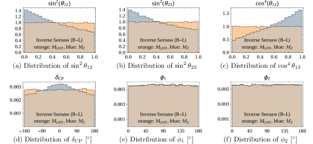
Refer to caption
Figure 11: Distributions of the mixing angles and physical CP phases before and after renormalization group running in the inverse seesaw model with gauged BL𝐵𝐿B-L. The orange regions correspond to the parameters at MGUTsubscript𝑀GUTM_{\text{GUT}},h scale, the blue regions to the parameters at MZsubscript𝑀𝑍M_{Z}. We find that the distributions are practically identical to those in the phenomenological inverse seesaw model from section III.2, see fig. 7.
Refer to caption
Figure 12: Shifts in the mixing angles and the CP phases during RG evolution form MGUTsubscript𝑀GUTM_{\text{GUT}} to MZsubscript𝑀𝑍M_{Z} in the inverse seesaw model with gauged BL𝐵𝐿B-L, obtained from 105superscript10510^{5} randomly generated mass matrices. We use the notation Δxx(MZ)x(MGUT)Δ𝑥𝑥subscript𝑀𝑍𝑥subscript𝑀GUT\Delta x\equiv x(M_{Z})-x(M_{\text{GUT}}), where x𝑥x stands for any of the mixing angles or complex phases. Also shown are Gaussian fits with central values Δx¯¯Δ𝑥\overline{\Delta x} and widths σ(Δx)𝜎Δ𝑥\sigma(\Delta x). The distributions are practically identical to those in the phenomenological inverse seesaw model from section III.2, see fig. 8.

Proceeding as we did in sections III.1 and III.2, we investigate how the statistical distributions of the neutrino mixing parameters change due to RG effects in the inverse seesaw model with gauged BL𝐵𝐿B-L. We generate 105superscript10510^{5} parameter sets at MGUTsubscript𝑀GUTM_{\text{GUT}} and evolve them down to MZsubscript𝑀𝑍M_{Z}. In fig. 11 we show the distributions of the mixing parameters before and after running, and in fig. 12 we plot the distributions of the RG-induced shifts ΔxΔ𝑥\Delta x. We find that these distributions are practically identical to those in the phenomenological inverse seesaw model without gauged BL𝐵𝐿B-L number. Consequently, also the value of P~KSsubscript~𝑃KS\tilde{P}_{\text{KS}} describing the compatibility of the data with anarchy is similar: 60.4%, compared to 59.3% in the phenomenological model. The running of the light neutrino masses is somewhat larger than in the phenomenological model, though: the average anomalous dimensions is -0.051, corresponding to a decrease of the mass eigenvalues by 80%.

IV Summary and Conclusions

In summary, we have studied how renormalization group effects alter the predictions of neutrino anarchy. We have found that the mixing angles at MZsubscript𝑀𝑍M_{Z} are on average several degrees smaller than at MGUTsubscript𝑀GUTM_{\text{GUT}}, and that the statistical distribution of the Dirac CP phase δCPsubscript𝛿CP\delta_{\text{CP}} after RG running peaks at zero. The Kolmogorov–Smirnov p𝑝p-value describing the compatibility of the observed mixing angles with the anarchy hypothesis thus increases from 41.1% without RG running to 47.7% with RG running in the type-I seesaw model, to 59.3% with RG running in the phenomenological inverse seesaw model, and to 60.4% with RG running in the inverse seesaw model with gauged BL𝐵𝐿B-L. Our results thus strengthen the claim that anarchy offers a good description of neutrino oscillation data, and they demonstrate that RG effects are crucial and need to be taken into account when deriving quantitative predictions in the anarchy scenario.

Acknowledgments

It is a pleasure to thank André de Gouvea, Jörn Kersten, and Hitoshi Murayama for useful discussions. We are moreover grateful to Alexander Merle for help in generating fig. 6, based on his papers [43, 44]. The work of VB and JK is supported by the German Research Foundation (DFG) under Grant Nos. KO 4820/1–1 and FOR 2239 and by the European Research Council (ERC) under the European Union’s Horizon 2020 research and innovation programme (grant agreement No. 637506, “ν𝜈\nuDirections”). VB and MK are supported by the DFG Graduate School Symmetry Breaking in Fundamental Interactions (GRK 1581). Additional support has been provided by the Cluster of Excellence “Precision Physics, Fundamental Interactions and Structure of Matter” (PRISMA – EXC 1098), grant No. 05H12UME of the German Federal Ministry for Education and Research (BMBF).

Appendix A Renormalization group equations for the type-I seesaw and inverse seesaw models

In this appendix, we list the renormalization group equations for the inverse seesaw model discussed in section III.2. By simply setting certain terms to zero in these equations, also the RG equations for the type-I seesaw will follow (see section A.3).

A.1 Structure of the mass matrix

We start from the mass matrix of the inverse seesaw model, eq. (18), which we repeat here:

Mν(0YνTv/20Yνv/20MDT0MDms).subscript𝑀𝜈matrix0subscriptsuperscript𝑌𝑇𝜈𝑣20subscript𝑌𝜈𝑣20subscriptsuperscript𝑀𝑇𝐷0subscript𝑀𝐷subscript𝑚𝑠\displaystyle M_{\nu}\equiv\begin{pmatrix}0&Y^{T}_{\nu}v/\sqrt{2}&0\\ Y_{\nu}v/\sqrt{2}&0&M^{T}_{D}\\ 0&M_{D}&m_{s}\end{pmatrix}\,. (21)

For 3 generations of active neutrinos, nNsubscript𝑛𝑁n_{N} generations of heavy NRsubscript𝑁𝑅N_{R} fields, and nSsubscript𝑛𝑆n_{S} generations of S𝑆S fields, Yνsubscript𝑌𝜈Y_{\nu} is an nN×3subscript𝑛𝑁3n_{N}\times 3 matrix, MDsubscript𝑀𝐷M_{D} is an nS×nNsubscript𝑛𝑆subscript𝑛𝑁n_{S}\times n_{N} matrix, and mssubscript𝑚𝑠m_{s} is an nS×nSsubscript𝑛𝑆subscript𝑛𝑆n_{S}\times n_{S} matrix. We assume Yν𝒪(1)similar-tonormsubscript𝑌𝜈𝒪1\|Y_{\nu}\|\sim\mathcal{O}(1), MDTeVsimilar-tonormsubscript𝑀𝐷TeV\|M_{D}\|\sim\text{TeV} and mskeVsimilar-tonormsubscript𝑚𝑠keV\|m_{s}\|\sim\text{keV}. We moreover assume nS>nNsubscript𝑛𝑆subscript𝑛𝑁n_{S}>n_{N} so that Mνsubscript𝑀𝜈M_{\nu} has at least one 𝒪(keV)𝒪keV\mathcal{O}(\text{keV}) eigenvalue, providing a dark matter candidate.

For the RG analysis, it is more convenient to work with a matrix which has diagonal elements much larger than the off-diagonal ones. Moreover, it is convenient to group the elements of this matrix by their typical scale. We therefore apply a unitary transformation V𝑉V to Mνsubscript𝑀𝜈M_{\nu} to bring it to the form

M~νVTMνV=(0Y^νTv/2Y~νTv/2Y^νv/2MNmDTY~νv/2mDm^s).subscript~𝑀𝜈superscript𝑉𝑇subscript𝑀𝜈𝑉matrix0subscriptsuperscript^𝑌𝑇𝜈𝑣2subscriptsuperscript~𝑌𝑇𝜈𝑣2subscript^𝑌𝜈𝑣2subscript𝑀𝑁subscriptsuperscript𝑚𝑇𝐷subscript~𝑌𝜈𝑣2subscript𝑚𝐷subscript^𝑚𝑠\displaystyle\tilde{M}_{\nu}\equiv V^{T}M_{\nu}V=\begin{pmatrix}0&\hat{Y}^{T}_{\nu}v/\sqrt{2}&\tilde{Y}^{T}_{\nu}v/\sqrt{2}\\ \hat{Y}_{\nu}v/\sqrt{2}&M_{N}&m^{T}_{D}\\ \tilde{Y}_{\nu}v/\sqrt{2}&m_{D}&\hat{m}_{s}\end{pmatrix}\,. (22)

V𝑉V is chosen such that MNmDmuch-greater-thannormsubscript𝑀𝑁normsubscript𝑚𝐷\|M_{N}\|\gg\|m_{D}\|, m^skeV\|\hat{m}_{s}\sim\text{keV}\| and Y^νYνY~νsimilar-tonormsubscript^𝑌𝜈normsubscript𝑌𝜈much-greater-thannormsubscript~𝑌𝜈\|\hat{Y}_{\nu}\|\sim\|Y_{\nu}\|\gg\|\tilde{Y}_{\nu}\|. Thus, MNsubscript𝑀𝑁M_{N} is a 2nN×2nN2subscript𝑛𝑁2subscript𝑛𝑁2n_{N}\times 2n_{N} matrix with eigenvalues of order TeV and m^ssubscript^𝑚𝑠\hat{m}_{s} is an (nSnN)×(nSnN)subscript𝑛𝑆subscript𝑛𝑁subscript𝑛𝑆subscript𝑛𝑁(n_{S}-n_{N})\times(n_{S}-n_{N}) matrix.

To construct V𝑉V explicitly, we first consider the unitary nS×nSsubscript𝑛𝑆subscript𝑛𝑆n_{S}\times n_{S} matrix uLsubscript𝑢𝐿u_{L} and the unitary nN×nNsubscript𝑛𝑁subscript𝑛𝑁n_{N}\times n_{N} matrix uRsubscript𝑢𝑅u_{R} which diagonalize MDsubscript𝑀𝐷M_{D} according to

MDdiag=uLMDuR.superscriptsubscript𝑀𝐷diagsuperscriptsubscript𝑢𝐿subscript𝑀𝐷subscript𝑢𝑅\displaystyle M_{D}^{\text{diag}}=u_{L}^{\dagger}M_{D}u_{R}\,. (23)

Here MDdiagsuperscriptsubscript𝑀𝐷diagM_{D}^{\text{diag}} means the diagonal matrix of eigenvalues, ordered in descending order. From uLsubscript𝑢𝐿u_{L} and uRsubscript𝑢𝑅u_{R}, we construct

ULsubscript𝑈𝐿\displaystyle U_{L} =(𝟏3+nN00uL)absentmatrixsubscript13subscript𝑛𝑁00subscript𝑢𝐿\displaystyle=\begin{pmatrix}\mathbf{1}_{3+n_{N}}&0\\ 0&u_{L}\end{pmatrix} URsubscript𝑈𝑅\displaystyle U_{R} =(𝟏3000uR000𝟏nS)absentmatrixsubscript13000subscript𝑢𝑅000subscript1subscript𝑛𝑆\displaystyle=\begin{pmatrix}\mathbf{1}_{3}&0&0\\ 0&u_{R}&0\\ 0&0&\mathbf{1}_{n_{S}}\end{pmatrix} W𝑊\displaystyle W =URUL.absentsubscript𝑈𝑅superscriptsubscript𝑈𝐿\displaystyle=U_{R}U_{L}^{*}\,. (24)

Then, the transformation

WTMνWsuperscript𝑊𝑇subscript𝑀𝜈𝑊\displaystyle W^{T}M_{\nu}W (25)

will diagonalize the MDsubscript𝑀𝐷M_{D} blocks in mνsubscript𝑚𝜈m_{\nu}, putting the largest mass eigenvalues on top. After this, we perform a rotation by π/4𝜋4\pi/4 in the singlet block, given by:

X𝑋\displaystyle X =(𝟏3000rnN×nNrnN×nS0rnS×nNrnS×nS),absentmatrixsubscript13000subscript𝑟subscript𝑛𝑁subscript𝑛𝑁subscript𝑟subscript𝑛𝑁subscript𝑛𝑆0subscript𝑟subscript𝑛𝑆subscript𝑛𝑁subscript𝑟subscript𝑛𝑆subscript𝑛𝑆\displaystyle=\begin{pmatrix}\mathbf{1}_{3}&0&0\\ 0&r_{n_{N}\times n_{N}}&r_{n_{N}\times n_{S}}\\ 0&-r_{n_{S}\times n_{N}}&r_{n_{S}\times n_{S}}\end{pmatrix}\,, (26)

where

rn×m12(10000100)subscript𝑟𝑛𝑚12matrix10000100\displaystyle r_{n\times m}\equiv\frac{1}{\sqrt{2}}\begin{pmatrix}1&\cdots&0&0&\cdots&0\\ \vdots&\ddots&\vdots&\vdots&\ddots&\vdots\\ 0&\cdots&1&0&\cdots&0\end{pmatrix} (27)

is the n×n𝑛𝑛n\times n identity matrix (multiplied by 1/2121/\sqrt{2}), padded with zeroes to turn it into an n×m𝑛𝑚n\times m matrix. After applying the full rotation

VURULX𝑉subscript𝑈𝑅superscriptsubscript𝑈𝐿𝑋\displaystyle V\equiv U_{R}U_{L}^{*}X (28)

to Mνsubscript𝑀𝜈M_{\nu}, we obtain M~νsubscript~𝑀𝜈\tilde{M}_{\nu} in the form given in eq. (22). We summarize the dimensions and the mass scales for the different blocks of Mνsubscript𝑀𝜈M_{\nu} and M~νsubscript~𝑀𝜈\tilde{M}_{\nu} in table 2. The 2nN×2nN2subscript𝑛𝑁2subscript𝑛𝑁2n_{N}\times 2n_{N} matrix MNsubscript𝑀𝑁M_{N} has nNsubscript𝑛𝑁n_{N} pairs of eigenvalues that differ only by ΔM𝒪(keV)similar-toΔ𝑀𝒪keV\Delta M\sim\mathcal{O}(\text{keV}), much less than the absolute scale of the eigenvalues of order TeV. The eigenstates in each pair couple to the active neutrinos via Yukawa couplings that are equal (up to a factor of i𝑖i). Their contributions to the light neutrino masses therefore cancel up to terms of order ΔM/MNΔ𝑀normsubscript𝑀𝑁\Delta M/\|M_{N}\|. This explains the smallness of the active neutrino masses despite the fact that Y^νsubscript^𝑌𝜈\hat{Y}_{\nu} is 𝒪(1)𝒪1\mathcal{O}(1) and MNsubscript𝑀𝑁M_{N} is 𝒪(TeV)𝒪TeV\mathcal{O}(\mathrm{TeV}). Another small contribution to the active neutrino masses comes from the 𝒪(keV)𝒪keV\mathcal{O}(\text{keV}) mass eigenstate mixing with the active fields through the strongly suppressed Y~νsubscript~𝑌𝜈\tilde{Y}_{\nu}. We can also understand why Mνsubscript𝑀𝜈M_{\nu} has nSnNsubscript𝑛𝑆subscript𝑛𝑁n_{S}-n_{N} eigenvalues of order keV: the off-diagonal elements in the last nSnNsubscript𝑛𝑆subscript𝑛𝑁n_{S}-n_{N} rows and columns of X𝑋X are zero and thus we get nSnNsubscript𝑛𝑆subscript𝑛𝑁n_{S}-n_{N} keV states that do not mix with the NRsubscript𝑁𝑅N_{R} or νLsubscript𝜈𝐿\nu_{L} fields.

Original basis Rotated basis
matrix dimensions matrix dimensions scale
Yνsubscript𝑌𝜈Y_{\nu} nN×3subscript𝑛𝑁3n_{N}\times 3 Y^νsubscript^𝑌𝜈\hat{Y}_{\nu} 2nN×32subscript𝑛𝑁32n_{N}\times 3 𝒪(Yν)𝒪subscript𝑌𝜈\mathcal{O}(Y_{\nu})
MDsubscript𝑀𝐷M_{D} nS×nNsubscript𝑛𝑆subscript𝑛𝑁n_{S}\times n_{N} Y~νsubscript~𝑌𝜈\tilde{Y}_{\nu} (nSnN)×3subscript𝑛𝑆subscript𝑛𝑁3(n_{S}-n_{N})\times 3 𝒪(Yνms/MD)𝒪subscript𝑌𝜈subscript𝑚𝑠subscript𝑀𝐷\mathcal{O}(Y_{\nu}m_{s}/M_{D})
mssubscript𝑚𝑠m_{s} nS×nSsubscript𝑛𝑆subscript𝑛𝑆n_{S}\times n_{S} MNsubscript𝑀𝑁M_{N} 2nN×2nN2subscript𝑛𝑁2subscript𝑛𝑁2n_{N}\times 2n_{N} 𝒪(MD)𝒪subscript𝑀𝐷\mathcal{O}(M_{D})
mDsubscript𝑚𝐷m_{D} (nSnN)×2nNsubscript𝑛𝑆subscript𝑛𝑁2subscript𝑛𝑁(n_{S}-n_{N})\times 2n_{N} 𝒪(ms)𝒪subscript𝑚𝑠\mathcal{O}(m_{s})
m^ssubscript^𝑚𝑠\hat{m}_{s} (nSnN)×(nSnN)subscript𝑛𝑆subscript𝑛𝑁subscript𝑛𝑆subscript𝑛𝑁(n_{S}-n_{N})\times(n_{S}-n_{N}) 𝒪(ms)𝒪subscript𝑚𝑠\mathcal{O}(m_{s})
Table 2: Dimensions of the submatrices forming the mass matrices Mνsubscript𝑀𝜈M_{\nu} and M~νsubscript~𝑀𝜈\tilde{M}_{\nu} in the inverse seesaw model (see eqs. 21 and 22). In the last column, we indicate the typical mass scale of the matrices in the rotated basis, eq. 22.

A.2 Beta functions for the inverse seesaw model

We derive the RG equation for the mass matrix M~νsubscript~𝑀𝜈\tilde{M}_{\nu} given in eq. 22 by using the fact that M~νsubscript~𝑀𝜈\tilde{M}_{\nu} has exactly the same structure as the mass matrix of a type-I seesaw model.

Whenever the renormalization scale μ𝜇\mu crosses the mass scale of one of the heavy sterile neutrinos as it is evolved from MGUTsubscript𝑀GUTM_{\text{GUT}} to MZsubscript𝑀𝑍M_{Z}, the corresponding row and column is removed from the mass matrix M~νsubscript~𝑀𝜈\tilde{M}_{\nu}. Moreover the remaining rows and columns are modified to include the effect of integrating out one neutrino state. This in particular implies that the upper 3×3333\times 3 block of M~νsubscript~𝑀𝜈\tilde{M}_{\nu}, which is zero initially, becomes a nonzero matrix κ𝜅\kappa. (We follow the notation of ref. [21] here.) If we did run down to sub-keV scales and integrated out all sterile states, κ𝜅\kappa would eventually coincide with mν=v22YνTMD1msMD1Yνsubscript𝑚𝜈superscript𝑣22superscriptsubscript𝑌𝜈𝑇superscriptsubscript𝑀𝐷1subscript𝑚𝑠superscriptsubscript𝑀𝐷1subscript𝑌𝜈m_{\nu}=\frac{v^{2}}{2}Y_{\nu}^{T}M_{D}^{-1}m_{s}M_{D}^{-1}Y_{\nu}.

For the β𝛽\beta functions of a parameter x𝑥x, we use the convention

βx=μddμx.subscript𝛽𝑥𝜇𝑑𝑑𝜇𝑥\displaystyle\beta_{x}=\mu\frac{d}{d\mu}x\,. (29)

The evolution equations read

16π2βMN16superscript𝜋2subscript𝛽subscript𝑀𝑁\displaystyle 16\pi^{2}\beta_{M_{N}} =(Y^νY^ν)MN+MN(Y^νY^ν)T+(Y^νY~ν)mD+mDT(Y^νY~ν)Tabsentsubscript^𝑌𝜈superscriptsubscript^𝑌𝜈subscript𝑀𝑁subscript𝑀𝑁superscriptsubscript^𝑌𝜈superscriptsubscript^𝑌𝜈𝑇subscript^𝑌𝜈superscriptsubscript~𝑌𝜈subscript𝑚𝐷superscriptsubscript𝑚𝐷𝑇superscriptsubscript^𝑌𝜈superscriptsubscript~𝑌𝜈𝑇\displaystyle=\big{(}\hat{Y}_{\nu}\hat{Y}_{\nu}^{\dagger}\big{)}M_{N}+M_{N}\big{(}\hat{Y}_{\nu}\hat{Y}_{\nu}^{\dagger}\big{)}^{T}+\big{(}\hat{Y}_{\nu}\tilde{Y}_{\nu}^{\dagger}\big{)}m_{D}+m_{D}^{T}\big{(}\hat{Y}_{\nu}\tilde{Y}_{\nu}^{\dagger}\big{)}^{T} (30)
16π2βm^s16superscript𝜋2subscript𝛽subscript^𝑚𝑠\displaystyle 16\pi^{2}\beta_{\hat{m}_{s}} =(Y~νY~ν)m^s+m^s(Y~νY~ν)T+(Y~νY^ν)mDT+mD(Y~νY^ν)Tabsentsubscript~𝑌𝜈superscriptsubscript~𝑌𝜈subscript^𝑚𝑠subscript^𝑚𝑠superscriptsubscript~𝑌𝜈superscriptsubscript~𝑌𝜈𝑇subscript~𝑌𝜈superscriptsubscript^𝑌𝜈superscriptsubscript𝑚𝐷𝑇subscript𝑚𝐷superscriptsubscript~𝑌𝜈superscriptsubscript^𝑌𝜈𝑇\displaystyle=\big{(}\tilde{Y}_{\nu}\tilde{Y}_{\nu}^{\dagger}\big{)}\hat{m}_{s}+\hat{m}_{s}\big{(}\tilde{Y}_{\nu}\tilde{Y}_{\nu}^{\dagger}\big{)}^{T}+\big{(}\tilde{Y}_{\nu}\hat{Y}_{\nu}^{\dagger}\big{)}m_{D}^{T}+m_{D}\big{(}\tilde{Y}_{\nu}\hat{Y}_{\nu}^{\dagger}\big{)}^{T} (31)
16π2βmD16superscript𝜋2subscript𝛽subscript𝑚𝐷\displaystyle 16\pi^{2}\beta_{m_{D}} =(Y~νY~ν)mD+mD(Y^νY^ν)T+(Y~νY^ν)M+m^s(Y^νY~ν)Tabsentsubscript~𝑌𝜈superscriptsubscript~𝑌𝜈subscript𝑚𝐷subscript𝑚𝐷superscriptsubscript^𝑌𝜈superscriptsubscript^𝑌𝜈𝑇subscript~𝑌𝜈superscriptsubscript^𝑌𝜈𝑀subscript^𝑚𝑠superscriptsubscript^𝑌𝜈superscriptsubscript~𝑌𝜈𝑇\displaystyle=\big{(}\tilde{Y}_{\nu}\tilde{Y}_{\nu}^{\dagger}\big{)}m_{D}+m_{D}\big{(}\hat{Y}_{\nu}\hat{Y}_{\nu}^{\dagger}\big{)}^{T}+\big{(}\tilde{Y}_{\nu}\hat{Y}_{\nu}^{\dagger}\big{)}M+\hat{m}_{s}\big{(}\hat{Y}_{\nu}\tilde{Y}_{\nu}^{\dagger}\big{)}^{T} (32)
16π2βκ16superscript𝜋2subscript𝛽𝜅\displaystyle 16\pi^{2}\beta_{\kappa} =32(YeYe)Tκ32κ(YeYe)+12(Y^νY^ν)Tκ+12κ(Y^νY^ν)absent32superscriptsuperscriptsubscript𝑌𝑒subscript𝑌𝑒𝑇𝜅32𝜅superscriptsubscript𝑌𝑒subscript𝑌𝑒12superscriptsuperscriptsubscript^𝑌𝜈subscript^𝑌𝜈𝑇𝜅12𝜅superscriptsubscript^𝑌𝜈subscript^𝑌𝜈\displaystyle=-\frac{3}{2}\big{(}Y_{e}^{\dagger}Y_{e}\big{)}^{T}\kappa-\frac{3}{2}\kappa\big{(}Y_{e}^{\dagger}Y_{e}\big{)}+\frac{1}{2}\big{(}\hat{Y}_{\nu}^{\dagger}\hat{Y}_{\nu}\big{)}^{T}\kappa+\frac{1}{2}\kappa\big{(}\hat{Y}_{\nu}^{\dagger}\hat{Y}_{\nu}\big{)}
+2tr(YeYe)κ+2tr(YνYν)κ+6tr(YuYu)κ2trsuperscriptsubscript𝑌𝑒subscript𝑌𝑒𝜅2trsuperscriptsubscript𝑌𝜈subscript𝑌𝜈𝜅6trsuperscriptsubscript𝑌𝑢subscript𝑌𝑢𝜅\displaystyle\quad+2\,\text{tr}\big{(}Y_{e}^{\dagger}Y_{e}\big{)}\kappa+2\,\text{tr}\big{(}Y_{\nu}^{\dagger}Y_{\nu}\big{)}\kappa+6\,\text{tr}\big{(}Y_{u}^{\dagger}Y_{u}\big{)}\kappa
+6tr(YdYd)κ3g22κ+λκ6trsuperscriptsubscript𝑌𝑑subscript𝑌𝑑𝜅3superscriptsubscript𝑔22𝜅𝜆𝜅\displaystyle\quad+6\,\text{tr}\big{(}Y_{d}^{\dagger}Y_{d}\big{)}\kappa-3g_{2}^{2}\kappa+\lambda\kappa (33)
16π2βY^ν16superscript𝜋2subscript𝛽subscript^𝑌𝜈\displaystyle 16\pi^{2}\beta_{\hat{Y}_{\nu}} =Y^ν[32(Y~νY~ν+Y^νY^ν)32(YeYe)+tr(Y^νY^ν+Y~νY~ν)\displaystyle=\hat{Y}_{\nu}\bigg{[}\frac{3}{2}\big{(}\tilde{Y}_{\nu}^{\dagger}\tilde{Y}_{\nu}+\hat{Y}_{\nu}^{\dagger}\hat{Y}_{\nu}\big{)}-\frac{3}{2}\big{(}Y_{e}^{\dagger}Y_{e}\big{)}+\text{tr}\big{(}\hat{Y}_{\nu}^{\dagger}\hat{Y}_{\nu}+\tilde{Y}_{\nu}^{\dagger}\tilde{Y}_{\nu}\big{)}
+tr(YeYe)+3tr(YuYu)+3tr(YdYd)920g1294g22]\displaystyle\qquad\ +\text{tr}\big{(}Y_{e}^{\dagger}Y_{e}\big{)}+3\,\text{tr}\big{(}Y_{u}^{\dagger}Y_{u}\big{)}+3\,\text{tr}\big{(}Y_{d}^{\dagger}Y_{d}\big{)}-\frac{9}{20}g_{1}^{2}-\frac{9}{4}g_{2}^{2}\bigg{]} (34)
16π2βY~ν16superscript𝜋2subscript𝛽subscript~𝑌𝜈\displaystyle 16\pi^{2}\beta_{\tilde{Y}_{\nu}} =Y~ν[32(Y~νY~ν+Y^νY^ν)32(YeYe)+tr(Y^νY^ν+Y~νY~ν)\displaystyle=\tilde{Y}_{\nu}\bigg{[}\frac{3}{2}\big{(}\tilde{Y}_{\nu}^{\dagger}\tilde{Y}_{\nu}+\hat{Y}_{\nu}^{\dagger}\hat{Y}_{\nu}\big{)}-\frac{3}{2}\big{(}Y_{e}^{\dagger}Y_{e}\big{)}+\text{tr}\big{(}\hat{Y}_{\nu}^{\dagger}\hat{Y}_{\nu}+\tilde{Y}_{\nu}^{\dagger}\tilde{Y}_{\nu}\big{)}
+tr(YeYe)+3tr(YuYu)+3tr(YdYd)920g1294g22]\displaystyle\qquad\ +\text{tr}\big{(}Y_{e}^{\dagger}Y_{e}\big{)}+3\,\text{tr}\big{(}Y_{u}^{\dagger}Y_{u}\big{)}+3\,\text{tr}\big{(}Y_{d}^{\dagger}Y_{d}\big{)}-\frac{9}{20}g_{1}^{2}-\frac{9}{4}g_{2}^{2}\bigg{]} (35)
16π2βYe16superscript𝜋2subscript𝛽subscript𝑌𝑒\displaystyle 16\pi^{2}\beta_{Y_{e}} =Ye[32YeYe32(Y^νY^ν+Y~νY~ν)94g1294g22\displaystyle=Y_{e}\bigg{[}\frac{3}{2}Y_{e}^{\dagger}Y_{e}-\frac{3}{2}\big{(}\hat{Y}_{\nu}^{\dagger}\hat{Y}_{\nu}+\tilde{Y}_{\nu}^{\dagger}\tilde{Y}_{\nu}\big{)}-\frac{9}{4}g_{1}^{2}-\frac{9}{4}g_{2}^{2}
+tr[YeYe+Y^νY^ν+Y~νY~ν+3YdYd+3YuYu]]\displaystyle\qquad\ +\text{tr}\big{[}Y_{e}^{\dagger}Y_{e}+\hat{Y}_{\nu}^{\dagger}\hat{Y}_{\nu}+\tilde{Y}_{\nu}^{\dagger}\tilde{Y}_{\nu}+3Y_{d}^{\dagger}Y_{d}+3Y_{u}^{\dagger}Y_{u}\big{]}\bigg{]} (36)
16π2βYd16superscript𝜋2subscript𝛽subscript𝑌𝑑\displaystyle 16\pi^{2}\beta_{Y_{d}} =Yd[32YdYd32YuYu14g1294g228g32\displaystyle=Y_{d}\bigg{[}\frac{3}{2}Y_{d}^{\dagger}Y_{d}-\frac{3}{2}Y_{u}^{\dagger}Y_{u}-\frac{1}{4}g_{1}^{2}-\frac{9}{4}g_{2}^{2}-8g_{3}^{2}
+tr[YeYe+Y^νY^ν+Y~νY~ν+3YdYd+3YuYu]]\displaystyle\qquad\ +\text{tr}\big{[}Y_{e}^{\dagger}Y_{e}+\hat{Y}_{\nu}^{\dagger}\hat{Y}_{\nu}+\tilde{Y}_{\nu}^{\dagger}\tilde{Y}_{\nu}+3Y_{d}^{\dagger}Y_{d}+3Y_{u}^{\dagger}Y_{u}\big{]}\bigg{]} (37)
16π2βYu16superscript𝜋2subscript𝛽subscript𝑌𝑢\displaystyle 16\pi^{2}\beta_{Y_{u}} =Yu[32YuYu32YdYd1720g1294g228g32\displaystyle=Y_{u}\bigg{[}\frac{3}{2}Y_{u}^{\dagger}Y_{u}-\frac{3}{2}Y_{d}^{\dagger}Y_{d}-\frac{17}{20}g_{1}^{2}-\frac{9}{4}g_{2}^{2}-8g_{3}^{2}
+tr[YeYe+Y^νY^ν+Y~νY~ν+3YdYd+3YuYu]]\displaystyle\qquad\ +\text{tr}\big{[}Y_{e}^{\dagger}Y_{e}+\hat{Y}_{\nu}^{\dagger}\hat{Y}_{\nu}+\tilde{Y}_{\nu}^{\dagger}\tilde{Y}_{\nu}+3Y_{d}^{\dagger}Y_{d}+3Y_{u}^{\dagger}Y_{u}\big{]}\bigg{]} (38)
16π2βλ16superscript𝜋2subscript𝛽𝜆\displaystyle 16\pi^{2}\beta_{\lambda} =6λ23λ(3g22+35g12)+3g24+32(35g12+g22)2absent6superscript𝜆23𝜆3superscriptsubscript𝑔2235superscriptsubscript𝑔123superscriptsubscript𝑔2432superscript35superscriptsubscript𝑔12superscriptsubscript𝑔222\displaystyle=6\lambda^{2}-3\lambda\bigg{(}3g_{2}^{2}+\frac{3}{5}g_{1}^{2}\bigg{)}+3g_{2}^{4}+\frac{3}{2}\bigg{(}\frac{3}{5}g_{1}^{2}+g_{2}^{2}\bigg{)}^{2}
+4λtr[YeYe+Y^νY^ν+Y~νY~ν+3YdYd+3YuYu]4𝜆trdelimited-[]superscriptsubscript𝑌𝑒subscript𝑌𝑒superscriptsubscript^𝑌𝜈subscript^𝑌𝜈superscriptsubscript~𝑌𝜈subscript~𝑌𝜈3superscriptsubscript𝑌𝑑subscript𝑌𝑑3superscriptsubscript𝑌𝑢subscript𝑌𝑢\displaystyle\quad+4\lambda\,\text{tr}\big{[}Y_{e}^{\dagger}Y_{e}+\hat{Y}_{\nu}^{\dagger}\hat{Y}_{\nu}+\tilde{Y}_{\nu}^{\dagger}\tilde{Y}_{\nu}+3Y_{d}^{\dagger}Y_{d}+3Y_{u}^{\dagger}Y_{u}\big{]}
8tr[YeYeYeYe+(Y^νY^ν+Y~νY~ν)(Y^νY^ν+Y~νY~ν)\displaystyle\quad-8\,\text{tr}\big{[}Y_{e}^{\dagger}Y_{e}Y_{e}^{\dagger}Y_{e}+\big{(}\hat{Y}_{\nu}^{\dagger}\hat{Y}_{\nu}+\tilde{Y}_{\nu}^{\dagger}\tilde{Y}_{\nu}\big{)}\big{(}\hat{Y}_{\nu}^{\dagger}\hat{Y}_{\nu}+\tilde{Y}_{\nu}^{\dagger}\tilde{Y}_{\nu}\big{)}
+3YdYdYdYd+3YuYuYuYu]\displaystyle\qquad\ +3Y_{d}^{\dagger}Y_{d}Y_{d}^{\dagger}Y_{d}+3Y_{u}^{\dagger}Y_{u}Y_{u}^{\dagger}Y_{u}\big{]} (39)

Note that the new fields introduced in the inverse seesaw model are all singlets under the SM gauge group. Therefore, the one-loop running of the SU(3)c×SU(2)L×U(1)Y𝑆𝑈subscript3𝑐𝑆𝑈subscript2𝐿𝑈subscript1𝑌SU(3)_{c}\times SU(2)_{L}\times U(1)_{Y} gauge couplings is described by the SM expressions

g12(μ)subscriptsuperscript𝑔21𝜇\displaystyle g^{-2}_{1}(\mu) =g12(MZ)4180π2log(μMZ),absentsuperscriptsubscript𝑔12subscript𝑀𝑍4180superscript𝜋2𝜇subscript𝑀𝑍\displaystyle=g_{1}^{-2}(M_{Z})-\frac{41}{80\pi^{2}}\log\bigg{(}\frac{\mu}{M_{Z}}\bigg{)}\,, (40)
g22(μ)subscriptsuperscript𝑔22𝜇\displaystyle g^{-2}_{2}(\mu) =g22(MZ)+1948π2log(μMZ),absentsuperscriptsubscript𝑔22subscript𝑀𝑍1948superscript𝜋2𝜇subscript𝑀𝑍\displaystyle=g_{2}^{-2}(M_{Z})+\frac{19}{48\pi^{2}}\log\bigg{(}\frac{\mu}{M_{Z}}\bigg{)}\,, (41)
g32(μ)subscriptsuperscript𝑔23𝜇\displaystyle g^{-2}_{3}(\mu) =g32(MZ)+78π2log(μMZ).absentsuperscriptsubscript𝑔32subscript𝑀𝑍78superscript𝜋2𝜇subscript𝑀𝑍\displaystyle=g_{3}^{-2}(M_{Z})+\frac{7}{8\pi^{2}}\log\bigg{(}\frac{\mu}{M_{Z}}\bigg{)}\,. (42)

A.3 Beta functions for the type-I seesaw model

By comparing the mass matrix of the inverse seesaw model, eq. 22, to the mass matrix of the type-I seesaw model

Mν,type-I(0YνTv/2Yνv/2M),subscript𝑀𝜈type-Imatrix0subscriptsuperscript𝑌𝑇𝜈𝑣2subscript𝑌𝜈𝑣2𝑀\displaystyle M_{\nu,\text{type-I}}\equiv\begin{pmatrix}0&Y^{T}_{\nu}v/\sqrt{2}\\ Y_{\nu}v/\sqrt{2}&M\\ \end{pmatrix}\,, (43)

we can immediately read off that the RGEs for the type-I seesaw model are obtained from eqs. 30 to 42 by setting Y^ν=Yνsubscript^𝑌𝜈subscript𝑌𝜈\hat{Y}_{\nu}=Y_{\nu}, MN=Msubscript𝑀𝑁𝑀M_{N}=M, Y~ν=0subscript~𝑌𝜈0\tilde{Y}_{\nu}=0, mD=0subscript𝑚𝐷0m_{D}=0, and m^s=0subscript^𝑚𝑠0\hat{m}_{s}=0.

Appendix B Beta functions in the inverse seesaw model with gauged BL𝐵𝐿B-L

For the model with the gauged U(1)BL𝑈subscript1𝐵𝐿U(1)_{B-L} symmetry, described in section III.3, we find the following evolution equations:

16π2βYν16superscript𝜋2subscript𝛽subscript𝑌𝜈\displaystyle 16\pi^{2}\beta_{Y_{\nu}} =Yν[12λSTλS]+Yν[32YνYν32YeYe+tr(YeYe)+tr(YνYν)\displaystyle=Y_{\nu}\bigg{[}\frac{1}{2}\lambda_{S}^{T}\lambda_{S}^{*}\bigg{]}+Y_{\nu}\bigg{[}\frac{3}{2}Y_{\nu}^{\dagger}Y_{\nu}-\frac{3}{2}Y_{e}^{\dagger}Y_{e}+\text{tr}(Y_{e}^{\dagger}Y_{e})+\text{tr}(Y_{\nu}^{\dagger}Y_{\nu})
+3tr(YdYd)+3tr(YuYu)920g1294g226g2]\displaystyle\qquad+3\,\text{tr}(Y_{d}^{\dagger}Y_{d})+3\,\text{tr}(Y_{u}^{\dagger}Y_{u})-\frac{9}{20}g_{1}^{2}-\frac{9}{4}g_{2}^{2}-6g^{\prime 2}\bigg{]} (44)
16π2βYe16superscript𝜋2subscript𝛽subscript𝑌𝑒\displaystyle 16\pi^{2}\beta_{Y_{e}} =Ye[32YeYe32YνYν+tr(YeYe)+tr(YνYν)+3tr(YdYd)\displaystyle=Y_{e}\bigg{[}\frac{3}{2}Y_{e}^{\dagger}Y_{e}-\frac{3}{2}Y_{\nu}^{\dagger}Y_{\nu}+\text{tr}(Y_{e}^{\dagger}Y_{e})+\text{tr}(Y_{\nu}^{\dagger}Y_{\nu})+3\,\text{tr}(Y_{d}^{\dagger}Y_{d})
+3tr(YuYu)94g1294g226g2]\displaystyle\qquad+3\,\text{tr}(Y_{u}^{\dagger}Y_{u})-\frac{9}{4}g_{1}^{2}-\frac{9}{4}g_{2}^{2}-6g^{\prime 2}\bigg{]} (45)
16π2βλS16superscript𝜋2subscript𝛽subscript𝜆𝑆\displaystyle 16\pi^{2}\beta_{\lambda_{S}} =λS[tr(λSλS)+YνYνT+λSλS15g2]absentsubscript𝜆𝑆delimited-[]trsuperscriptsubscript𝜆𝑆subscript𝜆𝑆superscriptsubscript𝑌𝜈superscriptsubscript𝑌𝜈𝑇superscriptsubscript𝜆𝑆subscript𝜆𝑆15superscript𝑔2\displaystyle=\lambda_{S}\bigg{[}\text{tr}(\lambda_{S}^{\dagger}\lambda_{S})+Y_{\nu}^{\ast}Y_{\nu}^{T}+\lambda_{S}^{\dagger}\lambda_{S}-15g^{\prime 2}\bigg{]} (46)
16π2βYu16superscript𝜋2subscript𝛽subscript𝑌𝑢\displaystyle 16\pi^{2}\beta_{Y_{u}} =Yu[32YuYu32YdYd1720g1294g228g3223g2\displaystyle=Y_{u}\bigg{[}\frac{3}{2}Y_{u}^{\dagger}Y_{u}-\frac{3}{2}Y_{d}^{\dagger}Y_{d}-\frac{17}{20}g_{1}^{2}-\frac{9}{4}g_{2}^{2}-8g_{3}^{2}-\frac{2}{3}g^{\prime 2}
+tr(YeYe)+tr(YνYν)+3tr(YdYd)+3tr(YuYu)]\displaystyle\qquad\vphantom{\frac{3}{2}}+\text{tr}(Y_{e}^{\dagger}Y_{e})+\text{tr}(Y_{\nu}^{\dagger}Y_{\nu})+3\,\text{tr}(Y_{d}^{\dagger}Y_{d})+3\,\text{tr}(Y_{u}^{\dagger}Y_{u})\bigg{]} (47)
16π2βYd16superscript𝜋2subscript𝛽subscript𝑌𝑑\displaystyle 16\pi^{2}\beta_{Y_{d}} =Yd[32YdYd32YuYu14g1294g228g3223g2\displaystyle=Y_{d}\bigg{[}\frac{3}{2}Y_{d}^{\dagger}Y_{d}-\frac{3}{2}Y_{u}^{\dagger}Y_{u}-\frac{1}{4}g_{1}^{2}-\frac{9}{4}g_{2}^{2}-8g_{3}^{2}-\frac{2}{3}g^{\prime 2}
+tr(YeYe)+tr(YνYν)+3tr(YdYd)+3tr(YuYu)]\displaystyle\qquad\vphantom{\frac{3}{2}}+\text{tr}(Y_{e}^{\dagger}Y_{e})+\text{tr}(Y_{\nu}^{\dagger}Y_{\nu})+3\,\text{tr}(Y_{d}^{\dagger}Y_{d})+3\,\text{tr}(Y_{u}^{\dagger}Y_{u})\bigg{]} (48)
16π2βg16superscript𝜋2subscript𝛽superscript𝑔\displaystyle 16\pi^{2}\beta_{g^{\prime}} =Cg3absent𝐶superscript𝑔3\displaystyle=Cg^{\prime 3} (49)

The numerical coefficient C𝐶C in the beta function for the U(1)BL𝑈subscript1𝐵𝐿U(1)_{B-L} coupling constant gsuperscript𝑔g^{\prime} in the last line, eq. 49, depends on the number of fields in the model and is given by

C=23fermionsQBL2+13scalarsQBL2.𝐶23subscriptfermionssuperscriptsubscript𝑄𝐵𝐿213subscriptscalarssuperscriptsubscript𝑄𝐵𝐿2C=\frac{2}{3}\sum_{\text{fermions}}Q_{B-L}^{2}+\frac{1}{3}\sum_{\text{scalars}}Q_{B-L}^{2}\,. (50)

In our specific model, including four generations of S𝑆S and Ssuperscript𝑆S^{\prime} each, we find C=973𝐶973C=\frac{97}{3}. For only three generations of S𝑆S and Ssuperscript𝑆S^{\prime} fields, we would have found C=27𝐶27C=27 instead. The running of the quartic Higgs coupling λ𝜆\lambda and of the SM gauge couplings is the same as in the phenomenological inverse seesaw model at one-loop level, see previous section. Note that we neglect the running of all parameters in the scalar sector other than the quartic Higgs coupling. The running of these couplings influences the evolution of the mixing parameters only indirectly by modifying the U(1)BL𝑈subscript1𝐵𝐿U(1)_{B-L} breaking scale.

Where possible, we have checked that we reproduce the applicable terms in the renormalization group equations presented in ref. [45] for a U(1)BL𝑈subscript1𝐵𝐿U(1)_{B-L} extension of the SM with three right-handed neutrinos, but without an inverse seesaw mechanism.

References

  • [1] L. J. Hall, H. Murayama, and N. Weiner, Neutrino mass anarchy, Phys.Rev.Lett. 84 (2000) 2572–2575, [hep-ph/9911341].
  • [2] N. Haba and H. Murayama, Anarchy and hierarchy, Phys.Rev. D63 (2001) 053010, [hep-ph/0009174].
  • [3] A. de Gouvea and H. Murayama, Statistical test of anarchy, Phys.Lett. B573 (2003) 94–100, [hep-ph/0301050].
  • [4] J. Espinosa, Anarchy in the neutrino sector?, hep-ph/0306019.
  • [5] A. de Gouvea and H. Murayama, Neutrino Mixing Anarchy: Alive and Kicking, 1204.1249.
  • [6] J. Heeck and W. Rodejohann, Sterile neutrino anarchy, Phys. Rev. D87 (2013), no. 3 037301, [1211.5295].
  • [7] J. Gluza and R. Szafron, Real and complex random neutrino mass matrices and theta13, Phys.Rev. D85 (2012) 047701, [1111.7278]. v3: Discussion about 3+1 scenario extended, fig 5,6 added.
  • [8] K. Agashe, T. Okui, and R. Sundrum, A Common Origin for Neutrino Anarchy and Charged Hierarchies, Phys.Rev.Lett. 102 (2009) 101801, [0810.1277].
  • [9] G. Altarelli, F. Feruglio, I. Masina, and L. Merlo, Repressing Anarchy in Neutrino Mass Textures, JHEP 1211 (2012) 139, [1207.0587].
  • [10] G. Altarelli, F. Feruglio, and I. Masina, Models of neutrino masses: Anarchy versus hierarchy, JHEP 0301 (2003) 035, [hep-ph/0210342].
  • [11] D. L. Bennett, H. B. Nielsen, and I. Picek, Understanding Fine Structure Constants and Three Generations, Phys. Lett. B208 (1988) 275.
  • [12] J. F. Donoghue, K. Dutta, and A. Ross, Quark and lepton masses and mixing in the landscape, Phys. Rev. D73 (2006) 113002, [hep-ph/0511219].
  • [13] J. F. Donoghue, K. Dutta, A. Ross, and M. Tegmark, Likely values of the Higgs vev, Phys. Rev. D81 (2010) 073003, [0903.1024].
  • [14] S. Antusch, J. Kersten, M. Lindner, and M. Ratz, Running neutrino masses, mixings and CP phases: Analytical results and phenomenological consequences, Nucl. Phys. B674 (2003) 401–433, [hep-ph/0305273].
  • [15] A. de Gouvea and J. Jenkins, The Physical Range of Majorana Neutrino Mixing Parameters, Phys.Rev. D78 (2008) 053003, [0804.3627].
  • [16] X. Lu and H. Murayama, Neutrino Mass Anarchy and the Universe, JHEP 1408 (2014) 101, [1405.0547].
  • [17] M. Gonzalez-Garcia, M. Maltoni, and T. Schwetz, Updated fit to three neutrino mixing: status of leptonic CP violation, JHEP 1411 (2014) 052, [1409.5439].
  • [18] J. Bergstrom, D. Meloni, and L. Merlo, A Bayesian comparison of U(1) lepton flavour models, Phys.Rev. D89 (2014) 093021, [1403.4528].
  • [19] P. Minkowski, μeγ𝜇𝑒𝛾\mu\rightarrow e\gamma at a Rate of One Out of 1-Billion Muon Decays?, Phys.Lett. B67 (1977) 421.
  • [20] R. N. Mohapatra and G. Senjanović, Neutrino mass and spontaneous parity nonconservation, Phys. Rev. Lett. 44 (Apr, 1980) 912–915.
  • [21] S. Antusch, J. Kersten, M. Lindner, M. Ratz, and M. A. Schmidt, Running neutrino mass parameters in see-saw scenarios, JHEP 0503 (2005) 024, [hep-ph/0501272].
  • [22] J.-w. Mei, Running neutrino masses, leptonic mixing angles and CP-violating phases: From M(Z) to Lambda(GUT), Phys.Rev. D71 (2005) 073012, [hep-ph/0502015].
  • [23] J. Casas, J. Espinosa, A. Ibarra, and I. Navarro, General RG equations for physical neutrino parameters and their phenomenological implications, Nucl.Phys. B573 (2000) 652–684, [hep-ph/9910420].
  • [24] P. H. Chankowski and Z. Pluciennik, Renormalization group equations for seesaw neutrino masses, Phys.Lett. B316 (1993) 312–317, [hep-ph/9306333].
  • [25] T. Ohlsson and S. Zhou, Renormalization group running of neutrino parameters, Nature Commun. 5 (2014) 5153, [1311.3846].
  • [26] N. Haba, K. Kaneta, R. Takahashi, and Y. Yamaguchi, Accurate renormalization group analyses in neutrino sector, Nucl.Phys. B885 (2014) 180–195, [1402.4126].
  • [27] M. A. Schmidt, Renormalization group evolution in the type I+ II seesaw model, Phys. Rev. D76 (2007) 073010, [0705.3841]. [Erratum: Phys. Rev.D85,099903(2012)].
  • [28] Planck Collaboration, P. Ade et al., Planck 2013 results. XVI. Cosmological parameters, Astron.Astrophys. 571 (2014) A16, [1303.5076].
  • [29] GERDA Collaboration, M. Agostini et al., Results on Neutrinoless Double-β𝛽\beta Decay of 76Ge from Phase I of the GERDA Experiment, Phys.Rev.Lett. 111 (2013), no. 12 122503, [1307.4720].
  • [30] EXO-200 Collaboration Collaboration, J. Albert et al., Search for Majorana neutrinos with the first two years of EXO-200 data, Nature 510 (2014) 229–234, [1402.6956].
  • [31] Y. Huang and B.-Q. Ma, Constraints on absolute neutrino Majorana mass from current data, Universe 2 (2014), no. 3 65–71, [1407.4357].
  • [32] R. N. Mohapatra and J. W. F. Valle, Neutrino mass and baryon-number nonconservation in superstring models, Phys. Rev. D 34 (Sep, 1986) 1642–1645.
  • [33] R. N. Mohapatra, Mechanism for understanding small neutrino mass in superstring theories, Phys. Rev. Lett. 56 (Feb, 1986) 561–563.
  • [34] C. Carvajal, A. Dias, C. Nishi, and B. Sánchez-Vega, Axion Like Particles and the Inverse Seesaw Mechanism, 1503.03502.
  • [35] A. Dias, C. de S. Pires, P. Rodrigues da Silva, and A. Sampieri, A Simple Realization of the Inverse Seesaw Mechanism, Phys.Rev. D86 (2012) 035007, [1206.2590].
  • [36] A. Dias, C. de S. Pires, and P. R. da Silva, How the Inverse See-Saw Mechanism Can Reveal Itself Natural, Canonical and Independent of the Right-Handed Neutrino Mass, Phys.Rev. D84 (2011) 053011, [1107.0739].
  • [37] P. Dev and R. Mohapatra, TeV Scale Inverse Seesaw in SO(10) and Leptonic Non-Unitarity Effects, Phys.Rev. D81 (2010) 013001, [0910.3924].
  • [38] A. Abada, G. Arcadi, and M. Lucente, Dark Matter in the minimal Inverse Seesaw mechanism, 1406.6556.
  • [39] P. B. Dev and A. Pilaftsis, Light and Superlight Sterile Neutrinos in the Minimal Radiative Inverse Seesaw Model, 1212.3808.
  • [40] J. Bergstrom, M. Malinsky, T. Ohlsson, and H. Zhang, Renormalization group running of neutrino parameters in the inverse seesaw model, Phys.Rev. D81 (2010) 116006, [1004.4628].
  • [41] S. Khalil, TeV-scale gauged B-L symmetry with inverse seesaw mechanism, Phys.Rev. D82 (2010) 077702, [1004.0013].
  • [42] W. Emam and S. Khalil, Higgs and Z-prime phenomenology in B-L extension of the standard model at LHC, Eur.Phys.J. C52 (2007) 625–633, [0704.1395].
  • [43] M. Lindner, A. Merle, and W. Rodejohann, Improved limit on theta(13) and implications for neutrino masses in neutrino-less double beta decay and cosmology, Phys.Rev. D73 (2006) 053005, [hep-ph/0512143].
  • [44] A. Merle and W. Rodejohann, The Elements of the neutrino mass matrix: Allowed ranges and implications of texture zeros, Phys.Rev. D73 (2006) 073012, [hep-ph/0603111].
  • [45] L. Basso, S. Moretti, and G. M. Pruna, A Renormalisation Group Equation Study of the Scalar Sector of the Minimal B-L Extension of the Standard Model, Phys.Rev. D82 (2010) 055018, [1004.3039].