Efficient inference in occlusion-aware generative models of images

Abstract

We present a generative model of images based on layering, in which image layers are individually generated, then composited from front to back. We are thus able to factor the appearance of an image into the appearance of individual objects within the image — and additionally for each individual object, we can factor content from pose. Unlike prior work on layered models, we learn a shape prior for each object/layer, allowing the model to tease out which object is in front by looking for a consistent shape, without needing access to motion cues or any labeled data. We show that ordinary stochastic gradient variational bayes (SGVB), which optimizes our fully differentiable lower-bound on the log-likelihood, is sufficient to learn an interpretable representation of images. Finally we present experiments demonstrating the effectiveness of the model for inferring foreground and background objects in images.

1 Introduction

Recently computer vision has made great progress by training deep feedforward neural networks on large labeled datasets. However, acquiring labeled training data for all of the problems that we care about is expensive. Furthermore, some problems require top-down inference as well as bottom-up inference in order to handle ambiguity. For example, consider the problem of object detection and instance segmentation in the presence of clutter/occlusion., as illustrated in Figure 1. In this case, the foreground object may obscure almost all of the background object, yet people are still able to detect that there are two objects present, to correctly segment out both of them, and even to amodally complete the hidden parts of the occluded object (cf., Kar et al. (2015)).

Figure 1: Illustration of occlusion.

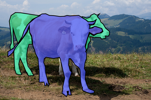
One way to tackle this problem is to use generative models. In particular, we can imagine the following generative process for an image: (1) Choose an object (or texture) of interest, by sampling a “content vector” representing its class label, style, etc; (2) Choose where to place the object in the 2d image plane, by sampling a “pose vector”, representing location, scale, etc. (3) Render an image of the object onto a hidden canvas or layer; (4) Repeat this process for $N$ objects (we assume in this work that $N$ is fixed); (5) Finally, generate the observed image by compositing the layers in order.

There have been several previous attempts to use layered generative models to perform scene parsing and object detection in clutter (see Section 2 for a review of related work). However, such methods usually run into computational bottlenecks, since inverting such generative models is intractable. In this paper, we build on recent work (primarily Kingma & Welling (2014); Gregor et al. (2015)) that shows how to jointly train a generative model and an inference network in a way that optimizes a variational lower bound on the log likelihood of the data; this has been called a “variational auto-encoder” or VAE. In particular, we extend this prior work in two ways. First, we extend it to the sequential setting, where we generate the observed image in stages by compositing hidden layers from front to back. Second, we combine the VAE with the spatial transformer network of (Jaderberg et al., 2015), allowing us to factor out variations in pose (e.g., location) from variations in content (e.g., identity). We call our model the “composited spatially transformed VAE”, or CST-VAE for short.

Our resulting inference algorithm combines top-down (generative) and bottom-up (discriminative) components in an interleaved fashion as follows: (1) First we recognize (bottom-up) the foreground object, factoring apart pose and content; (2) Having recognized it, we generate (top-down) what the hidden image should look like; (3) Finally, we virtually remove this generated hidden image from the observed image to get the residual image, and we repeat the process. (This is somewhat reminiscent of approaches that the brain is believed to use, Hochstein & Ahissar (2002).)

The end result is a way to factor an observed image of overlapping objects into $N$ hidden layers, where each layer contains a single object with its pose parameters. Remarkably, this whole process can be trained in a fully unsupervised way using standard gradient-based optimization methods (see Section 3 for details). In Section 4, we show that our method is able to reliably interpret cluttered images, and that the inferred latent representation is a much better feature vector for a discriminative classification task than working with the original cluttered images.

2 Related work

2.1 Deep probabilistic generative models

Our approach is inspired by the recent introduction of generative deep learning models that can be trained end-to-end using backpropagation. These models have included generative adversarial networks (Denton et al., 2015; Goodfellow et al., 2014) as well as variational auto-encoder (VAE) models (Kingma & Welling, 2014; Kingma et al., 2014; Rezende et al., 2014; Burda et al., 2015) which are most relevant to our setting.

Among the variational auto-encoder literature, our work is most comparable to the DRAW network of Gregor et al. (2015). As with our proposed model, the DRAW network is a generative model of images in the variational auto-encoder framework that decomposes image formation into multiple stages of additions to a canvas matrix. The DRAW paper assumes an LSTM based generative model of these sequential drawing actions which is more general than our model. In practice, these drawing actions seem to progressively refine an initially blurry region of an image to be sharper. In our work, we also construct the image sequentially, but each step is encouraged to correspond to a layer in the image, similar to what one might have in typical photo editing software. This encourages our hidden stochastic variable to be interpretable, which could potentially be useful for semi-supervised learning.

2.2 Modeling Transformation in neural networks

One of our major contributions is a model that is capable of separating the pose of an object from its appearance, which is of course a classic problem in computer vision. Here we highlight several of the most related works from the deep learning community. Many of these related works have been influenced by the Transforming Auto-encoder models by Hinton et al. (2011), in which pose is explicitly separated from content in an auto-encoder which is trained to predict (known) small transformations of an image. More recently, Dosovitskiy et al. (2015) introduced a convolutional network to generate images of chairs where pose was explicitly separated out, and Cheung et al. (2014) introduced an auto-encoder where a subset of variables such as pose can be explicitly observed and remaining variables are encouraged to explain orthogonal factors of variation. Most relevant in this line of works is that of Kulkarni et al. (2015), which, like us, separate the content of an image from pose parameters using a variational auto-encoder. In all of these works, however, there is an element of supervision, where variables such as pose and lighting are known at training time. Our method, which is based on the recently introduced Spatial Transformer Networks paper  (Jaderberg et al., 2015), is able to separate pose from content in an fully unsupervised setting using standard off-the-shelf gradient methods.

2.3 Layered models of images

Layer models of images is an old idea. Most works take advantage of motion cues to decompose video data into layers (Darrell & Pentland, 1991; Wang & Adelson, 1994; Ayer & Sawhney, 1995; Kannan et al., 2005; 2008). However, there have been some papers that work from single images. Yang et al. (2012), for example, propose a layered model for segmentation but rely heavily on bounding box and categorical annotations. Isola & Liu (2013) deconstruct a single image into layers, but require a training set of manually segmented regions. Our generative model is similar to that proposed by Williams & Titsias (2004), however we can capture more complex appearance models by using deep neural networks, compared to their per-pixel mixture-of-gaussian models. Moreover, our training procedure is simpler since it is just end-to-end minibatch SGD. Our approach also has similarities to the work of Le Roux et al. (2011), however they use restricted Boltzmann machines, which require expensive MCMC sampling to estimate gradients and have difficulties reliably estimating the log-partition function.

3 CST-VAE: A probabilistic layered model of image generation

Figure 2: 2 Cartoon illustration of the CST-VAE layer compositing process; 2 CST-VAE graphical model.

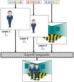
In this section we introduce the Composited Spatially Transformed Variational Auto-encoder (CST-VAE), a family of latent variable models, which factors the appearance of an image into the appearance of the different layers that create that image. Among other things, the CST-VAE model allows us to tease apart the component layers (or objects) that make up an image and reason about occlusion in order to perform tasks such as amodal completion (Kar et al., 2015) or instance segmentation (Hariharan et al., 2014). Furthermore, it can be trained in a fully unsupervised fashion using minibatch stochastic gradient descent methods but can also make use of labels in supervised or semi-supervised settings.

In the CST-VAE model, we assume that images are created by (1) generating a sequence of image layers, then (2) compositing the layers to form a final result. Figure 2 shows a simplified cartoon illustration of this process. We now discuss these two steps individually.

Layer generation via the ST-VAE model.

The layer generation model is interesting in its own right and we will call it the Spatially transformed Variational Auto-Encoder (ST-VAE) model (since there is no compositing step). We intuitively think of layers as corresponding to objects in a scene — a layer $L$ is assumed to be generated by first generating an image $C$ of an object in some canonical pose (we refer to this image as the canonical image for layer $L$), then warping $C$ in the 2d image plane (via some transformation $T$). We assume that both $C$ and $T$ are generated by some latent variable — specifically $C=f_{C}(z^{C};\theta_{C})$ and $T=f_{T}(z^{T};\theta_{T})$, where $z^{C}$ and $z^{T}$ are latent variables and $f_{C}(\cdot;\theta_{C})$ and $f_{T}(\cdot;\theta_{T})$ are nonlinear functions with parameters $\theta_{C}$ and $\theta_{T}$ to be learned. We will call these content and pose generators/decoders. We are agnostic as to the particular parameterizations of $f_{C}$ and $f_{T}$, though as we discuss below, they are assumed to be almost-everywhere differentiable and in practice we have used MLPs. In the interest of seeking simple interpretations of images, we also assume that these latent pose and content ($z^{C}$, $z^{T}$) variables are low-dimensional and independently Gaussian.

Finally to obtain the warped image, we use Spatial Transformer Network (STN) modules, recently introduced by Jaderberg et al. (2015). We will denote the result of resampling an image $C$ onto a regular grid which has been transformed by $T$ by $STN(C,T)$. The benefit of using STN modules in our setting is that they perform resampling in a differentiable way, allowing for our models to be trained using gradient methods.

Compositing.

To form the final observed image of the (general multi-layer) CST-VAE model, we generate a sequence of layers $L_{1}$, $L_{2}$, …, $L_{N}$ independently drawn from the ST-VAE model and composite from front to back. There are many ways to composite multiple layers in computer graphics (Porter & Duff, 1984). In our experiments, we use the classic over operator, which reduces to a simple $\alpha$-weighted convex combination of foreground and background pixels (denoted as a binary operation $\oplus$) in the two-layer setting, but can be iteratively applied to handle multiple layers.

To summarize, the CST-VAE model can be written as the following generative process. Let $x_{0}=\mathbf{0}^{w\times h}$ (i.e., a black image). For $i=1,\dots,N$:

$$z_{i}^{C},z_{i}^{T} \sim\mathcal{N}(0,I),$$

$$C_{i} =f_{C}(z_{i}^{C};\theta_{C}),$$

$$T_{i} =f_{T}(z_{i}^{T};\theta_{T}),$$

$$L_{i} =\mbox{STN}(C_{i},T_{i}),$$

$$x_{i} =x_{i-1}\oplus L_{i},$$

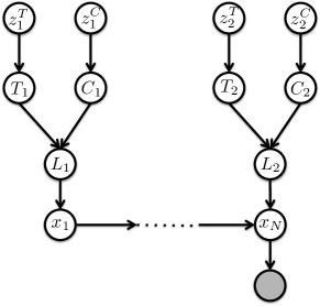
Finally, given $x_{N}$, we stochastically generate the observed image $x$ using $p(x|x_{N})$. If the image is binary, this is a Bernoulli model of the form $p(x^{j}=1|x_{N}^{j})=\mbox{Ber}(\sigma(x_{N}^{j}))$ for each pixel $j$; if the image is real-valued, we use a Gaussian model of the form $p(x^{j}=1|x_{N}^{j})={\cal N}(x_{N}^{j},\sigma^{2})$. See Figure 2 for a graphical model depiction of the CST-VAE generative model.

3.1 Inference and parameter learning with variational auto-encoders

In the context of the CST-VAE model, we are interested in two coupled problems: inference, by which we mean inferring all of the latent variables $z^{C}_{i}$ and $z^{T}_{i}$ given the model parameters $\theta$ and the image; and learning, by which we mean estimating the model parameters $\theta=\{\theta_{C},\theta_{T}\}$ given a training set of images $\{x^{(i)}\}_{i=1}^{m}$. Traditionally for latent variable models such as CST-VAE, one might solve these problems using EM  (Dempster et al., 1977), using approximate inference (e.g., loopy belief propagation, MCMC or mean-field) in the E-step (see e.g., Wainwright & Jordan (2008)). However if we want to allow for rich expressive parameterizations of the generative models $f_{C}$ and $f_{T}$, these approaches become intractable. Instead we use the recently proposed variational auto-encoder (VAE) framework (Kingma & Welling, 2014) for inference and learning.

In the variational auto-encoder setting, we assume that the posterior distribution over latents is parameterized by a particular form $Q(z^{C},z^{T}|\gamma)$, where $\gamma$ are data-dependent parameters. Rather than optimizing these at runtime, we compute them using an MLP, $\gamma=f_{enc}(x,\phi)$, which is called a recognition model or an encoder. We jointly optimize the generative model parameters $\theta$ and recognition model parameters $\phi$ by maximizing the following:

$$\mathcal{L}(\theta,\phi;\{x^{(i)}\}_{i=1}^{m})=\sum_{i=1}^{m}\frac{1}{S}\sum_{s=1}^{S}\left[-\log Q(z_{i,s}^{C},z_{i,s}^{T}|f_{enc}(x^{(i)},\phi))+\log P(x^{(i)}|z_{i,s}^{C},z_{i,s}^{T};\theta)\right],$$ (3.1)

where $z_{i,s}^{C},z_{i,s}^{T}\sim Q(z^{C},z^{T}|f_{enc}(x^{(i)};\phi))$ are samples drawn from the variational posterior $Q$, and $m$ is the size of the training set, and $S$ is the number of times we must sample the posterior per training example (in practice, we use $S=1$, following Kingma & Welling (2014)). We will use a diagonal multivariate Gaussian for $Q$, so that the recognition model just has to predict the mean and variance, $\mu(x;\phi)$ and $\sigma^{2}(x;\phi)$.

Equation 3.1 is stochastic lower bound on the observed data log-likelihood and interestingly, is differentiable with respect to parameters $\theta$ and $\phi$ in certain situations. In particular, when $Q$ is Gaussian and the likelihood under the generative model $P(x|z^{C},z^{T};\theta)$ is differentiable, then the stochastic variational lower bound can be written in an end-to-end differentiable way via the so-called reparameterization trick introduced in  Kingma & Welling (2014). Furthermore, the objective in Equation 3.1 can be interpreted as a reconstruction cost plus regularization term on the bottleneck portion of a neural network, which is why we think of these models as auto-encoders. In the following, we discuss how to do parameter learning and inference for the CST-VAE model more specifically. The critical design choice that must be made is how to parameterize the recognition model so that we can appropriately capture the important dependencies that may arise in the posterior.

3.2 Inference in the ST-VAE model

Figure 3: 3 ST-VAE Generative model, $P(L|z^{C},z^{T})$ (Decoder); 3 ST-VAE Recognition model $Q(z^{C},z^{T}|L)=Q(z^{C}|z^{T},L)\cdot Q(z^{T}|L)$ (Encoder)

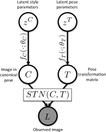
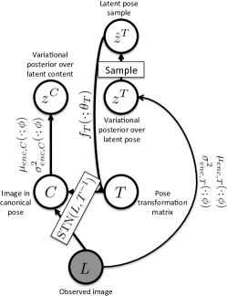
We focus first on how to parameterize the recognition network (encoder) for the simpler case of a single layer model (i.e., the ST-VAE model shown in Figure 3), in which we need only predict a single set of latent variables $z^{C}$ and $z^{T}$. Naïvely, one could simply use an ordinary MLP to parameterize a distribution $Q(z^{C},z^{T}|L)$, but ideally we would take advantage of the same insight that we used for the generative model, namely that it is easier to recognize content if we separately account for the pose. To this end, we propose the ST-VAE recognition model shown in Figure 3. Conceptually the ST-VAE recognition model breaks the prediction of $z^{C}$ and $z^{T}$ into two stages. Given the observed image $L$, we first predict the latent representation of the pose, $z^{T}$. Having this latent $z^{T}$ allows us to recover the pose transformation $T$ itself, which we use to “undo” the transformation of the generative process by using the Spatial Transformer Network again but this time with the inverse transformation of the predicted pose. This result, which can be thought of as a prediction of the image in a canonical pose, is finally used to predict latent content parameters.

More precisely, we assume that the joint posterior distribution over pose and content factors as $Q(z^{C},z^{T}|L)=Q(z^{T}|L)\cdot Q(z^{C}|z^{T},L)$ where both factors are normal distributions. To obtain a draw $(\hat{z}^{C},\hat{z}^{T})$ from this posterior, we use the following procedure:

$$\hat{z}^{T} \sim Q(z^{T}|L;\phi)=\mathcal{N}(\mu_{T}(L;\phi),\mbox{diag}(\sigma_{T}^{2}(L;\phi))),$$

$$\hat{T} =f_{T}(\hat{z}^{T};\theta_{T}),$$

$$\hat{C} =\mbox{STN}(L,\hat{T}^{-1}),$$

$$\hat{z}^{C} \sim Q(z^{C}|z^{T},L;\phi)=\mathcal{N}(\mu_{C}(\hat{C};\phi),\mbox{diag}(\sigma_{C}^{2}(\hat{C};\phi))),$$

where $f_{T}$ is the pose decoder from the ST-VAE generative model discussed above. To train an ST-VAE model, we then use the above parameterization of $Q$ and maximize Equation 3.1 with minibatch SGD. As long as the pose and content encoders and decoders are differentiable, Equation 3.1 is guaranteed to also be end-to-end differentiable.

3.3 Inference in the CST-VAE model

Figure 4: The CST-VAE network “unrolled” for two image layers.

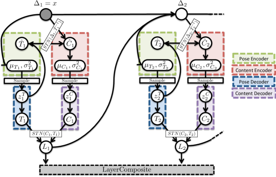
We now turn back to the multi-layer CST-VAE model, where again the task is to parameterize the recognition model $Q$. In particular we would like to avoid learning a model that must make a “straight-shot” joint prediction of all objects and their poses in an image. Instead our approach is to perform inference over a single layer at a time from front to back, each time removing the contribution of a layer from consideration until the last layer has been explained.

We proceed recursively: to perform inference for layer $L_{i}$, we assume that the latent parameters $z^{C}_{i}$ and $z^{T}_{i}$ are responsible for explaining some part of the residual image $\Delta_{i}$ — i.e. the part of image that has not been explained by layers $L_{1},\dots,L_{i-1}$ (note that $\Delta_{1}=x$). We then use the ST-VAE module (both the decoder and encoder modules) to generate a reconstruction of the layer $L_{i}$ given the current residual image $\Delta_{i}$. Finally to compute the next residual image to be explained by future layers, we set $\Delta_{i+1}=\max(0,\Delta_{i}-L_{i})$. We use the ReLU transfer function, $ReLU(\cdot)=\max(0,\cdot)$, to ensure that the residual image can always itself be interpreted as an image (since $\Delta_{i}-L_{i}$ can be negative, which breaks interpretability of the layers).

Note that our encoder for layer $L_{i}$ requires that the decoder has been run for layer $L_{i-1}$. Thus it’s not possible to separate the generative and recognition models into disjoint parts as in the ST-VAE model. Figure 4 unrolls the entire CST-VAE network (combining both generative and recognition models) for two layers.

4 Evaluation

In all of our experiments we use the same training settings used in Kingma & Welling (2014); that is, we use Adagrad for optimization with minibatches of 100 with a learning rate of 0.01 and a weight decay corresponding to a prior of $\mathcal{N}(0,1)$. We initialize weights in our network using the heuristic of  Glorot & Bengio (2010). However for the pose recognition modules in the ST-VAE model, we have found it useful to specifically initialize biases so that poses are initially close to the identity transformation (see Jaderberg et al. (2015)).

We use vanilla VAE models as a baseline model against first the (single image layer) ST-VAE model, then the more general CST-VAE model. In all of our comparison we fix the training time for all models. We experiment with between 20 and 50 dimensions for the latent content variables $z^{C}$ and always use 6 dimensions for pose variables $z^{T}$. We parameterize content encoders and decoders by using a two layer fully connected MLP with 256 dimensional hidden layers and ReLU nonlinearities. For pose decoders and encoders we also use two layer fully connected MLPs, but using 32 dimensional hidden layers and Tanh nonlinearities. Finally for spatial transformer modules, we always resample onto a grid that is the same size as the original image.

Figure 5: 5 Comparison of samples from the VAE and ST-VAE generative models. For the ST-VAE model, we show both the sample in its canonical pose and the final generated image. 5 Averaged images from each MNIST class as learning progresses — we typically see pose variables converge very quickly.

Train Accuracy Test Accuracy On translated (36x36) MNIST VAE + supervised 0.771 0.146 ST-VAE + supervised 0.972 0.964 directly supervised 0.884 0.783 Directly supervised with STN 0.993 0.969 On original (28x28) MNIST Directly supervised 0.999 0.96

Figure 6: 6 Train and test (per-example) lower bounds on log-likelihood for the vanilla VAE and ST-VAE models on the Translated MNIST data; 6 Classification accuracy obtained by supervised training using latent encodings from VAE and ST-VAE models. More details in text.

4.1 Evaluating the ST-VAE on images of single objects

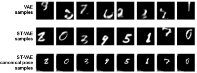
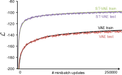
We first evaluate our ST-VAE (single image layer) model alone on the MNIST dataset (LeCun et al., 1998) and a derived dataset, TranslatedMNIST, in which we randomly translated each $28\times 28$ MNIST example within a $36\times 36$ black image. In both cases, we binarize the images by thresholding, as in Kingma & Welling (2014). Figure 6 plots train and test log-likelihoods over 250000 gradient steps comparing the vanilla VAE model against the ST-VAE model, where we see that from the beginning the ST-VAE model is able to achieve a much better likelihood while not overfitting. This can also be seen in Figure 5 which visualizes samples from both generative models. We see that while the VAE model (top row) manages to generate randomly transformed blobs on the image, these blobs typically only look somewhat like digits. For the ST-VAE model, we plot both the final samples (middle row) as well as the intermediate canonical images (last row), which typically are visually closer to MNIST digits.

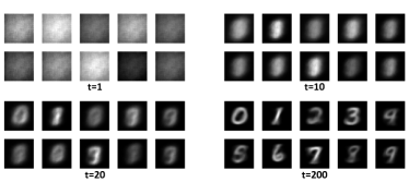
Interestingly, the canonical images tend to be slightly smaller versions of the digits and our model relies on the Spatial Transformer Networks to scale them up at the end of the generative process. Though we have not performed a careful investigation, possible reasons for this effect may be a combination of the fact (1) that scaling up the images introduces some blur which accounts for small variations in nearby pixels and (2) it is easier to encode smaller digits than larger ones. We also observe (Figure 5) that the pose network when trained on our dataset tends to converge rapidly, bringing digits to a centered canonical pose within tens of gradient updates. Once the digits have been aligned, the content network is able to make better progress.

Finally we evaluate the latent content codes $z^{C}$ learned by our ST-VAE model in digit classification using the standard MNIST train/test split. For this experiment we use a two layer MLP with 32 hidden units in each layer and ReLU nonlinearities applied to the posterior mean of $z^{C}$ inferred from each image; we do not use the labels to fine tune the VAE. Figure 6 summarizes the results, where we compare against three baseline classifiers: (1) an MLP learned on latent codes from the VAE model, (2) an MLP trained directly on Translated MNIST images (we call this the “directly supervised classifier”), and (3) the approach of Jaderberg et al. (2015) using the same MLP as above trained directly on images but with a spatial transformer network. As a point of reference, we also provide the performance of our classifier on the original $28\times 28$ MNIST dataset. We see that the ST-VAE model is able to learn a latent representation of image content that holds enough information to be competitive with the  Jaderberg et al. (2015) approach (both of which slightly outperform the MLP training directly on the original MNIST set). The approaches that do not account for pose variation do much worse than ST-VAE on this task and exhibit significant overfitting.

4.2 Evaluating the CST-VAE on images with multiple overlapping objects

Figure 7: 7 Train and test (per-example) lower bounds on log-likelihood for the vanilla VAE and CST-VAE models on the Superimposed MNIST data; 7 Classification accuracy obtained by supervised training using latent encodings from VAE and CST-VAE models. More details in text. 7 Images from the Superimposed MNIST dataset with visualizations of intermediate variables in the neural network corresponding to first and second image layers and the final reconstruction.

We now show results from the CST-VAE model on a challenging “Superimposed MNIST” dataset. We constructed this dataset by randomly translating then superimposing two MNIST digits one at a time onto $50\times 50$ black backgrounds, generating a total of 100,000 images for training and 50,000 for testing. A large fraction of the dataset thus consists of overlapping digits that occlude one another, sometimes so severely that a human is unable to classify the two digits in the image. In this section we use the same pose/content encoder and decoder architectures as above except that we set hidden content encoder/decoder layers to be 128-dimensional — empirically, we find that larger hidden layers tend to be sensitive to initialization for this model. We also assume that observed images are composited using two image layers (which can be thought of as foreground and background).

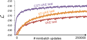
Figure 7 plots test log-likelihoods over 250000 gradient steps comparing the vanilla VAE model against the ST-VAE and CST-VAE model, where we see that from the beginning the CST-VAE model is able to achieve a much better solution than the ST-VAE model which in turn outperforms the VAE model. In this experiment, we ensure that the total number of latent dimensions across all models is similar. In particular, we allow the VAE and ST-VAE models to use 50 latent dimensions for content. The ST-VAE model uses an additional 6 dimensions for the latent pose. For the CST-VAE model we use 20 latent content dimensions and 6 latent pose dimensions per image layer $L_{i}$ (for a total of 52 latent dimensions).

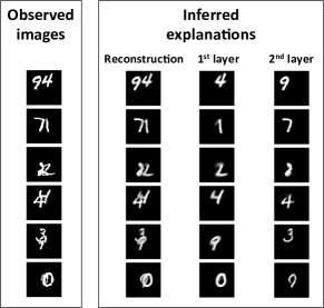
Figure 7 highlights the interpretability of our model. On the left column, we show example superimposed digits from our dataset and ask the CST-VAE to reconstruct them (second column). As a byproduct of this reconstruction, we are able to individually separate a foreground image (third column) and background image (fourth column), often corresponding to the correct digits that were used to generate the observation. While not perfect, the CST-VAE model manages to do well even on some challenging examples where digits exhibit high occlusion. To generate these foreground/background images, we use the posterior mean inferred by the network for each image layer $L_{i}$; however, we note that one of the advantages of the variational auto-encoder framework is that it is also able to represent uncertainty over different interpretations of the input image.

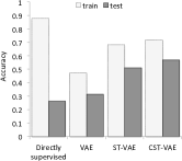
Finally, we evaluate our performance on classification. We use the same two layer MLP architecture (with 256 hidden layer units) as we did with the ST-VAE model, and train using latent representations learned by the CST-VAE model. Specifically we concatenate the latent content vectors $z^{C}_{1}$ and $z^{C}_{2}$ which are fed as input to the classifier network. As baselines we compare against (1) the vanilla VAE latent representations and (2) a classifier trained directly on images of superimposed digits. We report accuracy, requiring that the classifier be correct on both digits within an image.

Figure 7 visualizes the results. We see that the classifier that is trained directly on pixels exhibits severe overfitting and performs the worst. The three variational auto-encoder models also slightly overfit, but perform better, with the CST-VAE obtaining the best results, with almost twice the accuracy as the vanilla VAE model.

5 Conclusion

We have shown how to combine an old idea — of interpretable, generative, layered models of images — with modern techniques of deep learning, in order to tackle the challenging problem of intepreting images in the presence of occlusion in an entirely unsupervised fashion. We see this is as a crucial stepping stone to future work on deeper scene understanding, going beyond simple feedforward supervised prediction problems. In the future, we would like to apply our approach to real images, and possibly video. This will require extending our methods to use convolutional networks, and may also require some weak supervision (e.g., in the form of observed object class labels associated with layers) or curriculum learning to simplify the learning task.

Acknowledgments

We are grateful to Sergio Guadarrama and Rahul Sukthankar for reading and providing feedback on a draft of this paper.

References

- Ayer & Sawhney (1995) Ayer, Serge and Sawhney, Harpreet S. Layered representation of motion video using robust maximum-likelihood estimation of mixture models and mdl encoding. In Computer Vision, 1995. Proceedings., Fifth International Conference on, pp. 777–784. IEEE, 1995.
- Burda et al. (2015) Burda, Yuri, Grosse, Roger, and Salakhutdinov, Ruslan. Importance weighted autoencoders. arXiv preprint arXiv:1509.00519, 2015.
- Cheung et al. (2014) Cheung, Brian, Livezey, Jesse A, Bansal, Arjun K, and Olshausen, Bruno A. Discovering hidden factors of variation in deep networks. arXiv preprint arXiv:1412.6583, 2014.
- Darrell & Pentland (1991) Darrell, Trevor and Pentland, Alex. Robust estimation of a multi-layered motion representation. In Visual Motion, 1991., Proceedings of the IEEE Workshop on, pp. 173–178. IEEE, 1991.
- Dempster et al. (1977) Dempster, Arthur P, Laird, Nan M, and Rubin, Donald B. Maximum likelihood from incomplete data via the em algorithm. Journal of the royal statistical society. Series B (methodological), pp. 1–38, 1977.
- Denton et al. (2015) Denton, Emily, Chintala, Soumith, Szlam, Arthur, and Fergus, Rob. Deep generative image models using a laplacian pyramid of adversarial networks. arXiv preprint arXiv:1506.05751, 2015.
- Dosovitskiy et al. (2015) Dosovitskiy, Alexey, Springenberg, Jost Tobias, and Brox, Thomas. Learning to generate chairs with convolutional neural networks. In IEEE International Conference on Computer Vision and Pattern Recognition (CVPR), 2015.
- Glorot & Bengio (2010) Glorot, Xavier and Bengio, Yoshua. Understanding the difficulty of training deep feedforward neural networks. In International conference on artificial intelligence and statistics, pp. 249–256, 2010.
- Goodfellow et al. (2014) Goodfellow, Ian, Pouget-Abadie, Jean, Mirza, Mehdi, Xu, Bing, Warde-Farley, David, Ozair, Sherjil, Courville, Aaron, and Bengio, Yoshua. Generative adversarial nets. In Advances in Neural Information Processing Systems, pp. 2672–2680, 2014.
- Gregor et al. (2015) Gregor, Karol, Danihelka, Ivo, Graves, Alex, and Wierstra, Daan. Draw: A recurrent neural network for image generation. In Proceedings of The 32nd International Conference on Machine Learning, 2015.
- Hariharan et al. (2014) Hariharan, Bharath, Arbel, Pablo, Girshick, Ross, and Malik, Jitendra. Simultaneous detection and segmentation. In ECCV, 2014.
- Hinton et al. (2011) Hinton, Geoffrey E, Krizhevsky, Alex, and Wang, Sida D. Transforming auto-encoders. In Artificial Neural Networks and Machine Learning–ICANN 2011, pp. 44–51. Springer, 2011.
- Hochstein & Ahissar (2002) Hochstein, Shaul and Ahissar, Merav. View from the top: hierarchies and reverse hierarchies in the visual system. Neuron, 36(5):791–804, 5 December 2002.
- Isola & Liu (2013) Isola, P and Liu, Ce. Scene collaging: Analysis and synthesis of natural images with semantic layers. In ICCV, pp. 3048–3055, December 2013.
- Jaderberg et al. (2015) Jaderberg, Max, Simonyan, Karen, Zisserman, Andrew, and Kavukcuoglu, Koray. Spatial transformer networks. arXiv preprint arXiv:1506.02025, 2015.
- Kannan et al. (2005) Kannan, Anitha, Jojic, Nebojsa, and Frey, B. Generative model for layers of appearance and deformation. AIStats, 2005.
- Kannan et al. (2008) Kannan, Anitha, Jojic, Nebojsa, and Frey, Brendan J. Fast transformation-invariant component analysis. International Journal of Computer Vision, 77(1-3):87–101, 2008.
- Kar et al. (2015) Kar, A., Tulsiani, S., Carreira, J., and Malik, J. Amodal completion and size constancy in natural scenes. In Intl. Conf. on Computer Vision, 2015.
- Kingma & Welling (2014) Kingma, Diederik P. and Welling, Max. Auto-encoding variational bayes. In Proceedings of the Second International Conference on Learning Representations (ICLR 2014), April 2014.
- Kingma et al. (2014) Kingma, Diederik P, Mohamed, Shakir, Rezende, Danilo Jimenez, and Welling, Max. Semi-supervised learning with deep generative models. In Advances in Neural Information Processing Systems, pp. 3581–3589, 2014.
- Kulkarni et al. (2015) Kulkarni, Tejas D, Whitney, Will, Kohli, Pushmeet, and Tenenbaum, Joshua B. Deep convolutional inverse graphics network. In Neural Information Processing Systems (NIPS 2015), 2015.
- Le Roux et al. (2011) Le Roux, Nicolas, Heess, Nicolas, Shotton, Jamie, and Winn, John. Learning a generative model of images by factoring appearance and shape. Neural Computation, 23(3):593–650, 2011.
- LeCun et al. (1998) LeCun, Yann, Bottou, Léon, Bengio, Yoshua, and Haffner, Patrick. Gradient-based learning applied to document recognition. Proceedings of the IEEE, 86(11):2278–2324, 1998.
- Porter & Duff (1984) Porter, Thomas and Duff, Tom. Compositing digital images. ACM Siggraph Computer Graphics, 18(3):253–259, 1984.
- Rezende et al. (2014) Rezende, Danilo Jimenez, Mohamed, Shakir, and Wierstra, Daan. Stochastic backpropagation and approximate inference in deep generative models. In International Conference on Machine Learning (ICML 2015), 2014.
- Wainwright & Jordan (2008) Wainwright, Martin J and Jordan, Michael I. Graphical models, exponential families, and variational inference. Foundations and Trends® in Machine Learning, 1(1-2):1–305, 2008.
- Wang & Adelson (1994) Wang, John YA and Adelson, Edward H. Representing moving images with layers. Image Processing, IEEE Transactions on, 3(5):625–638, 1994.
- Williams & Titsias (2004) Williams, Christopher KI and Titsias, Michalis K. Greedy learning of multiple objects in images using robust statistics and factorial learning. Neural Computation, 16(5):1039–1062, 2004.
- Yang et al. (2012) Yang, Yi, Hallman, Sam, Ramanan, Deva, and Fowlkes, Charless C. Layered object models for image segmentation. Pattern Analysis and Machine Intelligence, IEEE Transactions on, 34(9):1731–1743, 2012.