The iterated auxiliary particle filter

Abstract

We present an offline, iterated particle filter to facilitate statistical inference in general state space hidden Markov models. Given a model and a sequence of observations, the associated marginal likelihood $L$ is central to likelihood-based inference for unknown statistical parameters. We define a class of “twisted” models: each member is specified by a sequence of positive functions $\bm{\psi}$ and has an associated $\bm{\psi}$-auxiliary particle filter that provides unbiased estimates of $L$. We identify a sequence $\bm{\psi}^{*}$ that is optimal in the sense that the $\bm{\psi}^{*}$-auxiliary particle filter’s estimate of $L$ has zero variance. In practical applications, $\bm{\psi}^{*}$ is unknown so the $\bm{\psi}^{*}$-auxiliary particle filter cannot straightforwardly be implemented. We use an iterative scheme to approximate $\bm{\psi}^{*}$, and demonstrate empirically that the resulting iterated auxiliary particle filter significantly outperforms the bootstrap particle filter in challenging settings. Applications include parameter estimation using a particle Markov chain Monte Carlo algorithm.

Keywords: Hidden Markov models, look-ahead methods, particle Markov chain Monte Carlo, sequential Monte Carlo, smoothing, state space models

1 Introduction

Particle filtering, or sequential Monte Carlo (SMC), methodology involves the simulation over time of an artificial particle system $(\xi_{t}^{i};\>t\in\left\{1,\dots,T\right\},\>i\in\{1,\ldots,N\})$. It is particularly suited to numerical approximation of integrals of the form

$$Z:=\int_{\mathsf{X}^{T}}\mu_{1}\left(x_{1}\right)g_{1}\left(x_{1}\right)\prod_{t=2}^{T}f_{t}\left(x_{t-1},x_{t}\right)g_{t}\left(x_{t}\right)dx_{1:T},$$ (1)

where $\mathsf{X}=\mathbb{R}^{d}$ for some $d\in\mathbb{N}$, $T\in\mathbb{N}$, $x_{1:T}:=(x_{1},\ldots,x_{T})$, $\mu_{1}$ is a probability density function on $\mathsf{X}$, each $f_{t}$ a transition density on $\mathsf{X}$, and each $g_{t}$ is a bounded, continuous and non-negative function. Algorithm 1 describes a particle filter, using which an estimate of (1) can be computed as

$$Z^{N}:=\prod_{t=1}^{T}\left[\frac{1}{N}\sum_{i=1}^{N}g_{t}(\xi_{t}^{i})\right].$$ (2)

Algorithm 1 A Particle Filter

1. Sample $\xi_{1}^{i}\sim\mu_{1}$ independently for $i\in\{1,\ldots,N\}$.

2. For $t=2,\ldots,T$, sample independently

   $$\xi_{t}^{i}\sim\frac{\sum_{j=1}^{N}g_{t-1}(\xi_{t-1}^{j})f_{t}(\xi_{t-1}^{j},\cdot)}{\sum_{j=1}^{N}g_{t-1}(\xi_{t-1}^{j})},\qquad i\in\{1,\ldots,N\}.$$

Particle filters were originally applied to statistical inference for hidden Markov models (HMMs) by Gordon et al. (1993), and this setting remains an important application. Letting $\mathsf{Y}=\mathbb{R}^{d^{\prime}}$ for some $d^{\prime}\in\mathbb{N}$, an HMM is a Markov chain evolving on $\mathsf{X}\times\mathsf{Y}$, $(X_{t},Y_{t})_{t\in\mathbb{N}}$, where $(X_{t})_{t\in\mathbb{N}}$ is itself a Markov chain and for $t\in\{1,\ldots,T\}$, each $Y_{t}$ is conditionally independent of all other random variables given $X_{t}$. In a time-homogeneous HMM, letting $\mathbb{P}$ denote the law of this bivariate Markov chain, we have

$$\mathbb{P}\left(X_{1:T}\in A,Y_{1:T}\in B\right):=\int_{A\times B}\mu\left(x_{1}\right)g\left(x_{1},y_{1}\right)\prod_{t=2}^{T}f\left(x_{t-1},x_{t}\right)g\left(x_{t},y_{t}\right)dx_{1:T}dy_{1:T},$$ (3)

where $\mu:\mathsf{X}\rightarrow\mathbb{R}_{+}$ is a probability density function, $f:\mathsf{X}\times\mathsf{X}\rightarrow\mathbb{R}_{+}$ a transition density, $g:\mathsf{X}\times\mathsf{Y}\rightarrow\mathbb{R}_{+}$ an observation density and $A$ and $B$ measurable subsets of $\mathsf{X}^{T}$ and $\mathsf{Y}^{T}$, respectively. Statistical inference is often conducted upon the basis of a realization $y_{1:T}$ of $Y_{1:T}$ for some finite $T$, which we will consider to be fixed throughout the remainder of the paper. Letting $\mathbb{E}$ denote expectations w.r.t. $\mathbb{P}$, our main statistical quantity of interest is $L:=\mathbb{E}\left[\prod_{t=1}^{T}g\left(X_{t},y_{t}\right)\right]$, the marginal likelihood associated with $y_{1:T}$. In the above, we take $\mathbb{R}_{+}$ to be the non-negative real numbers, and assume throughout that $L>0$.

Running Algorithm 1 with

$$\mu_{1}=\mu,\qquad f_{t}=f,\qquad g_{t}(x)=g(x,y_{t}),$$ (4)

corresponds exactly to running the bootstrap particle filter (BPF) of Gordon et al. (1993), and we observe that when (4) holds, the quantity $Z$ defined in (1) is identical to $L$, so that $Z^{N}$ defined in (2) is an approximation of $L$. In applications where $L$ is the primary quantity of interest, there is typically an unknown statistical parameter $\theta\in\Theta$ that governs $\mu$, $f$ and $g$, and in this setting the map $\theta\mapsto L(\theta)$ is the likelihood function. We continue to suppress the dependence on $\theta$ from the notation until Section 5.

The accuracy of the approximation $Z^{N}$ has been studied extensively. For example, the expectation of $Z^{N}$, under the law of the particle filter, is exactly $Z$ for any $N\in\mathbb{N}$, and $Z^{N}$ converges almost surely to $Z$ as $N\rightarrow\infty$; these can be seen as consequences of Del Moral (2004, Theorem 7.4.2). For practical values of $N$, however, the quality of the approximation can vary considerably depending on the model and/or observation sequence. When used to facilitate parameter estimation using, e.g., particle Markov chain Monte Carlo (Andrieu et al., 2010), it is desirable that the accuracy of $Z^{N}$ be robust to small changes in the model and this is not typically the case.

In Section 2 we introduce a family of “twisted HMMs”, parametrized by a sequence of positive functions $\bm{\psi}:=(\psi_{1},\ldots,\psi_{T})$. Running a particle filter associated with any of these twisted HMMs provides unbiased and strongly consistent estimates of $L$. Some specific definitions of $\bm{\psi}$ correspond to well-known modifications of the BPF, and the algorithm itself can be viewed as a generalization of the auxiliary particle filter (APF) of Pitt & Shephard (1999). Of particular interest is a sequence $\bm{\psi}^{*}$ for which $Z^{N}=L$ with probability $1$. In general, $\bm{\psi}^{*}$ is not known and the corresponding APF cannot be implemented, so our main focus in Section 3 is approximating the sequence $\bm{\psi}^{*}$ iteratively, and defining final estimates through use of a simple stopping rule. In the applications of Section 5 we find that the resulting estimates significantly outperform the BPF, and exhibit some robustness to both increases in the dimension of the latent state space $\mathsf{X}$ and changes in the model parameters. There are some restrictions on the class of transition densities and the functions $\psi_{1},\ldots,\psi_{T}$ that can be used in practice, which we discuss.

This work builds upon a number of methodological advances, most notably the twisted particle filter (Whiteley & Lee, 2014), the APF (Pitt & Shephard, 1999), block sampling (Doucet et al., 2006), and look-ahead schemes (Lin et al., 2013). In particular, the sequence $\bm{\psi}^{*}$ is closely related to the generalized eigenfunctions described in Whiteley & Lee (2014), but in that work the particle filter as opposed to the HMM was twisted to define alternative approximations of $L$. For simplicity, we have presented the BPF in which multinomial resampling occurs at each time step. Commonly employed modifications of this algorithm include adaptive resampling (Kong et al., 1994; Liu & Chen, 1995) and alternative resampling schemes (see, e.g., Douc et al., 2005). Generalization to the time-inhomogeneous HMM setting is fairly straightforward, so we restrict ourselves to the time-homogeneous setting for clarity of exposition.

2 Twisted models and the $\bm{\psi}$-auxiliary particle filter

Given an HMM $(\mu,f,g)$ and a sequence of observations $y_{1:T}$, we introduce a family of alternative twisted models based on a sequence of real-valued, bounded, continuous and positive functions $\boldsymbol{\psi}:=\left(\psi_{1},\psi_{2},\dots,\psi_{T}\right)$. Letting, for an arbitrary transition density $f$ and function $\psi$, $f(x,\psi):=\int_{\mathsf{X}}f\left(x,x^{\prime}\right)\psi\left(x^{\prime}\right)dx^{\prime}$, we define a sequence of normalizing functions $(\tilde{\psi}_{1},\tilde{\psi}_{2},\dots,\tilde{\psi}_{T})$ on $\mathsf{X}$ by $\tilde{\psi}_{t}(x_{t}):=f\left(x_{t},\psi_{t+1}\right)$ for $t\in\{1,\ldots,T-1\}$, $\tilde{\psi}_{T}\equiv 1$, and a normalizing constant $\tilde{\psi}_{0}:=\int_{\mathsf{X}}\mu\left(x_{1}\right)\psi_{1}\left(x_{1}\right)dx_{1}$. We then define the twisted model via the following sequence of twisted initial and transition densities

$$\mu_{1}^{\boldsymbol{\psi}}(x_{1}):=\frac{\mu(x_{1})\psi_{1}(x_{1})}{\tilde{\psi}_{0}},\qquad f_{t}^{\boldsymbol{\psi}}(x_{t-1},x_{t}):=\frac{f\left(x_{t-1},x_{t}\right)\psi_{t}\left(x_{t}\right)}{\tilde{\psi}_{t-1}\left(x_{t-1}\right)},\quad t\in\{2,\ldots,T\},$$ (5)

and the sequence of positive functions

$$g_{1}^{\boldsymbol{\psi}}\left(x_{1}\right):=g\left(x_{1},y_{1}\right)\frac{\tilde{\psi}_{1}\left(x_{1}\right)}{\psi_{1}\left(x_{1}\right)}\tilde{\psi}_{0},\qquad g_{t}^{\boldsymbol{\psi}}\left(x_{t}\right):=g\left(x_{t},y_{t}\right)\frac{\tilde{\psi}_{t}\left(x_{t}\right)}{\psi_{t}\left(x_{t}\right)},\quad t\in\{2,\ldots T\},$$ (6)

which play the role of observation densities in the twisted model. Our interest in this family is motivated by the following invariance result.

Proposition 1.

If $\boldsymbol{\psi}$ is a sequence of bounded, continuous and positive functions, and

$$Z_{\bm{\psi}}:=\int_{\mathsf{X}^{T}}\mu_{1}^{\bm{\psi}}\left(x_{1}\right)g_{1}^{\bm{\psi}}\left(x_{1}\right)\prod_{t=2}^{T}f_{t}^{\bm{\psi}}\left(x_{t-1},x_{t}\right)g_{t}^{\bm{\psi}}\left(x_{t}\right)dx_{1:T},$$

then $Z_{\bm{\psi}}=L$.

Proof.

We observe that

$$\mu_{1}^{\boldsymbol{\psi}}\left(x_{1}\right)g_{1}^{\boldsymbol{\psi}}\left(x_{1}\right)\prod_{t=2}^{T}f_{t}^{\boldsymbol{\psi}}\left(x_{t-1},x_{t}\right)g_{t}^{\boldsymbol{\psi}}\left(x_{t}\right)$$

$$= \frac{\mu(x_{1})\psi_{1}(x_{1})}{\tilde{\psi}_{0}}g_{1}\left(x_{1}\right)\frac{\tilde{\psi}_{1}\left(x_{1}\right)}{\psi_{1}\left(x_{1}\right)}\tilde{\psi}_{0}\cdot\prod_{t=2}^{T}\frac{f\left(x_{t-1},x_{t}\right)\psi_{t}\left(x_{t}\right)}{\tilde{\psi}_{t-1}\left(x_{t-1}\right)}g_{t}\left(x_{t}\right)\frac{\tilde{\psi}_{t}\left(x_{t}\right)}{\psi_{t}\left(x_{t}\right)}$$

$$= \mu\left(x_{1}\right)g_{1}\left(x_{1}\right)\prod_{t=2}^{T}f\left(x_{t-1},x_{t}\right)g_{t}\left(x_{t}\right),$$

and the result follows. ∎

From a methodological perspective, Proposition 1 makes clear a particular sense in which the L.H.S. of (1) is common to an entire family of $\mu_{1}$, $(f_{t})_{t\in\{2,\ldots,T\}}$ and $(g_{t})_{t\in\{1,\ldots,T\}}$. The BPF associated with the twisted model corresponds to choosing

$$\mu_{1}=\mu^{\bm{\psi}},\qquad f_{t}=f_{t}^{\bm{\psi}},\qquad g_{t}=g_{t}^{\bm{\psi}},$$ (7)

in Algorithm 1; to emphasize the dependence on $\bm{\psi}$, we provide in Algorithm 2 the corresponding algorithm and we will denote approximations of $L$ by $Z_{\bm{\psi}}^{N}$. We demonstrate below that the BPF associated with the twisted model can also be viewed as an APF associated with the sequence $\bm{\psi}$, and so refer to this algorithm as the $\bm{\psi}$-APF. Since the class of $\bm{\psi}$-APF’s is very large, it is natural to consider whether there is an optimal choice of $\bm{\psi}$, in terms of the accuracy of the approximation $Z_{\bm{\psi}}^{N}$: the following Proposition describes such a sequence.

Algorithm 2 $\bm{\psi}$-Auxiliary Particle Filter

1. Sample $\xi_{1}^{i}\sim\mu^{\bm{\psi}}$ independently for $i\in\{1,\ldots,N\}$.

2. For $t=2,\ldots,T$, sample independently

   $$\xi_{t}^{i}\sim\frac{\sum_{j=1}^{N}g_{t-1}^{\bm{\psi}}(\xi_{t-1}^{j})f_{t}^{\bm{\psi}}(\xi_{t-1}^{j},\cdot)}{\sum_{j=1}^{N}g_{t-1}^{\bm{\psi}}(\xi_{t-1}^{j})},\qquad i\in\{1,\ldots,N\}.$$

Proposition 2.

Let $\bm{\psi}^{*}:=(\psi_{1}^{*},\ldots,\psi_{T}^{*})$, where $\psi_{T}^{*}\left(x_{T}\right):=g(x_{T},y_{T})$, and

$$\psi_{t}^{*}\left(x_{t}\right):=g\left(x_{t},y_{t}\right)\mathbb{E}\left[\prod_{p=t+1}^{T}g\left(X_{p},y_{p}\right)\biggl{|}\left\{X_{t}=x_{t}\right\}\right],\quad x_{t}\in\mathsf{X},$$ (8)

for $t\in\{1,\ldots,T-1\}$. Then, $Z_{\bm{\psi}^{*}}^{N}=L$ with probability $1$.

Proof.

It can be established that

$$g(x_{t},y_{t})\tilde{\psi}_{t}^{*}(x_{t})=\psi_{t}^{*}(x_{t}),\qquad t\in\{1,\ldots,T\},\qquad x_{t}\in\mathsf{X},$$

and so we obtain from (6) that $g_{1}^{\boldsymbol{\psi}^{*}}\equiv\tilde{\psi}_{0}^{*}$ and $g_{t}^{\boldsymbol{\psi}^{*}}\equiv 1$ for $t\in\{2,\ldots,T\}$. Hence,

$$Z_{N}^{\boldsymbol{\psi}^{*}}=\prod_{t=1}^{T}\left[\frac{1}{N}\sum_{i=1}^{N}g_{t}^{\boldsymbol{\psi}^{*}}\left(\xi_{t}^{i}\right)\right]=\tilde{\psi}_{0}^{*},$$

with probability $1$. To conclude, we observe that

$$\tilde{\psi}_{0}^{*} = \int_{\mathsf{X}}\mu\left(x_{1}\right)\psi_{1}^{*}\left(x_{1}\right)dx_{1}=\int_{\mathsf{X}}\mu\left(x_{1}\right)\mathbb{E}\left[\prod_{t=1}^{T}g\left(X_{t},y_{t}\right)\biggl{|}\left\{X_{1}=x_{1}\right\}\right]dx_{1}$$

$$= \mathbb{E}\left[\prod_{t=1}^{T}g\left(X_{t},y_{t}\right)\right]=L.\qed$$

Implementation of Algorithm 2 requires that one can sample according to $\mu_{1}^{\bm{\psi}}$ and $f_{t}^{\bm{\psi}}(x,\cdot)$ and compute $g_{t}^{\boldsymbol{\psi}}$ pointwise. This imposes restrictions on the choice of $\bm{\psi}$ in practice, since one must be able to compute both $\psi_{t}$ and $\tilde{\psi}_{t}$ pointwise. In general models, the sequence $\bm{\psi}^{*}$ cannot be used for this reason as (8) cannot be computed explicitly. However, since Algorithm 2 is valid for any sequence of positive functions $\bm{\psi}$, we can interpret Proposition 2 as motivating the effective design of a particle filter by solving a sequence of function approximation problems.

Alternatives to the BPF have been considered before (see, e.g., the “locally optimal” proposal in Doucet et al. 2000 and the discussion in Del Moral 2004, Section 2.4.2). The family of particle filters we have defined using $\bm{\psi}$ are unusual, however, in that $g_{t}^{\bm{\psi}}$ is a function only of $x_{t}$ rather than $(x_{t-1},x_{t})$; other approaches in which the particles are sampled according to a transition density that is not $f$ typically require this extension of the domain of these functions. This is again a consequence of the fact that the $\bm{\psi}$-APF can be viewed as a BPF for a twisted model. This feature is shared by the fully adapted APF of Pitt & Shephard (1999), when recast as a standard particle filter for an alternative model as in Johansen & Doucet (2008), and which is obtained as a special case of Algorithm 2 when $\psi_{t}(\cdot)\equiv g(\cdot,y_{t})$ for each $t\in\{1,\ldots,T\}$. We view the approach here as generalizing that algorithm for this reason.

It is possible to recover other existing methodological approaches as BPFs for twisted models. In particular, when each element of $\bm{\psi}$ is a constant function, we recover the standard BPF of Gordon et al. (1993). Setting $\psi_{t}\left(x_{t}\right)=g\left(x_{t},y_{t}\right)$ gives rise to the fully adapted APF. By taking, for some $k\in\mathbb{N}$ and each $t\in\{1,\ldots,T\}$,

$$\psi_{t}\left(x_{t}\right) =g\left(x_{t},y_{t}\right)\mathbb{E}\left[\prod_{p=t+1}^{(t+k)\wedge T}g\left(X_{p},y_{p}\right)\biggl{|}\left\{X_{t}=x_{t}\right\}\right],\quad x_{t}\in\mathsf{X},$$ (9)

$\bm{\psi}$ corresponds to a sequence of look-ahead functions (see, e.g., Lin et al., 2013) and one can recover idealized versions of the delayed sample method of Chen et al. (2000) (see also the fixed-lag smoothing approach in Clapp & Godsill 1999), and the block sampling particle filter of Doucet et al. (2006). When $k\geq T-1$, we obtain the sequence $\bm{\psi}^{*}$. Just as $\bm{\psi}^{*}$ cannot typically be used in practice, neither can the exact look-ahead strategies obtained by using (9) for some fixed $k$. In such situations, the proposed look-ahead particle filtering strategies are not $\bm{\psi}$-APFs, and their relationship to the $\bm{\psi}^{*}$-APF is consequently less clear. We note that the offline setting we consider here affords us the freedom to define twisted models using the entire data record $y_{1:T}$. The APF was originally introduced to incorporate a single additional observation, and could therefore be implemented in an online setting, i.e. the algorithm could run while the data record was being produced.

3 Function approximations and the iterated APF

3.1 Asymptotic variance of the $\bm{\psi}$-APF

Since it is not typically possible to use the sequence $\bm{\psi}^{*}$ in practice, we propose to use an approximation of each member of $\bm{\psi}^{*}$. In order to motivate such an approximation, we provide a Central Limit Theorem, adapted from a general result due to Del Moral (2004, Chapter 9). It is convenient to make use of the fact that the estimate $Z_{\bm{\psi}}^{N}$ is invariant to rescaling of the functions $\psi_{t}$ by constants, and we adopt now a particular scaling that simplifies the expression of the asymptotic variance. In particular, we let

$$\bar{\psi}_{t}(x):=\frac{\psi_{t}(x)}{\mathbb{E}\left[\psi_{t}\left(X_{t}\right)\mid\left\{Y_{1:t-1}=y_{1:t-1}\right\}\right]},\qquad\bar{\psi}_{t}^{*}(x):=\frac{\psi_{t}^{*}(x)}{\mathbb{E}\left[\psi_{t}^{*}\left(X_{t}\right)\mid\left\{Y_{1:t-1}=y_{1:t-1}\right\}\right]}.$$

Proposition 3.

Let $\bm{\psi}$ be a sequence of bounded, continuous and positive functions. Then

$$\sqrt{N}\left(\frac{Z_{\bm{\psi}}^{N}}{Z}-1\right)\overset{d}{\longrightarrow}\mathcal{N}(0,\sigma_{\bm{\psi}}^{2}),$$

where,

$$\sigma_{\bm{\psi}}^{2}:=\sum_{t=1}^{T}\left\{\mathbb{E}\left[\frac{\bar{\psi}_{t}^{*}\left(X_{t}\right)}{\bar{\psi}_{t}\left(X_{t}\right)}\left|\vphantom{\frac{\psi_{t}^{*}\left(X_{t}\right)}{\psi_{t}\left(X_{t}\right)}}\right.\left\{\vphantom{\frac{\psi_{t}^{*}\left(X_{t}\right)}{\psi_{t}\left(X_{t}\right)}}Y_{1:T}=y_{1:T}\right\}\right]-1\right\}.$$ (10)

We emphasize that Proposition 3, whose proof can be found in the Appendix, follows straightforwardly from existing results for Algorithm 1, since the $\bm{\psi}$-APF can be viewed as a BPF for the twisted model defined by $\bm{\psi}$. For example, in the case $\bm{\psi}$ consists only of constant functions, we obtain the standard asymptotic variance for the BPF

$$\sigma^{2}=\sum_{t=1}^{T}\left\{\mathbb{E}\left[\bar{\psi}_{t}^{*}\left(X_{t}\right)\mid\left\{Y_{1:T}=y_{1:T}\right\}\right]-1\right\}.$$

From Proposition 3 we can deduce that $\sigma_{\bm{\psi}}^{2}$ tends to $0$ as $\bm{\psi}$ approaches $\bm{\psi}^{*}$ in an appropriate sense. Hence, Propositions 2 and 3 together provide some justification for designing particle filters by approximating the sequence $\bm{\psi}^{*}$.

3.2 Classes of $f$ and $\bm{\psi}$

While the $\bm{\psi}$-APF described in Section 2 and the asymptotic results just described are valid very generally, practical implementation of the $\bm{\psi}$-APF does impose some restrictions jointly on the transition densities $f$ and functions in $\bm{\psi}$. Here we consider only the case where the HMM’s initial distribution is a mixture of Gaussians and $f$ is a member of $\mathcal{F}$, the class of transition densities of the form

$$f\left(x,\cdot\right)=\sum_{k=1}^{M}c_{k}(x)\mathcal{N}\left(\>\cdot\>;a_{k}\left(x\right),b_{k}\left(x\right)\right),$$ (11)

where $M\in\mathbb{N}$, and $(a_{k})_{k\in\{1,\ldots,M\}}$ and $(b_{k})_{k\in\{1,\ldots,M\}}$ are sequences of mean and covariance functions, respectively and $(c_{k})_{k\in\{1,\ldots,M\}}$ a sequence of $\mathbb{R}_{+}$-valued functions with $\sum_{k=1}^{M}c_{k}(x)=1$ for all $x\in\mathsf{X}$. Let $\Psi$ define the class of functions of the form

$$\psi(x)=C+\sum_{k=1}^{M}c_{k}\mathcal{N}\left(x;a_{k},b_{k}\right),$$ (12)

where $M\in\mathbb{N}$, $C\in\mathbb{R}_{+}$, and $(a_{k})_{k\in\{1,\ldots,M\}}$, $(b_{k})_{k\in\{1,\ldots,M\}}$ and $(c_{k})_{k\in\{1,\ldots,M\}}$ are a sequence of means, covariances and positive real numbers, respectively. When $f\in\mathcal{F}$ and each $\psi_{t}\in\Psi$, it is straightforward to implement Algorithm 2 since, for each $t\in\{1,\ldots,T\}$, both $\psi_{t}(x)$ and $\tilde{\psi}_{t-1}(x)=f(x,\psi_{t})$ can be computed explicitly and $f_{t}^{\bm{\psi}}(x,\cdot)$ is a mixture of normal distributions whose component means and covariance matrices can also be computed. Alternatives to this particular setting are discussed in Section 6.

3.3 Recursive approximation of $\bm{\psi^{*}}$

The ability to compute $f(\cdot,\psi_{t})$ pointwise when $f\in\mathcal{F}$ and $\psi_{t}\in\Psi$ is also instrumental in the recursive function approximation scheme we now describe. Our approach is based on the following observation.

Proposition 4.

The sequence $\boldsymbol{\psi}^{*}$ satisfies $\psi_{T}^{*}\left(x_{T}\right)=g\left(x_{T},y_{T}\right)$, $x_{T}\in\mathsf{X}$ and

$$\psi_{t}^{*}\left(x_{t}\right)=g\left(x_{t},y_{t}\right)f\left(x_{t},\psi_{t+1}^{*}\right),\quad x_{t}\in\mathsf{X},\quad t\in\{1,\ldots,T-1\}.$$ (13)

Proof.

The definition of $\bm{\psi}^{*}$ provides that $\psi_{T}^{*}\left(x_{T}\right)=g\left(x_{T},y_{T}\right)$. For $t\in\{1,\ldots,T-1\}$,

$$g\left(x_{t},y_{t}\right)f\left(x_{t},\psi_{t+1}^{*}\right)$$

$$= g\left(x_{t},y_{t}\right)\int_{\mathsf{X}}f\left(x_{t},x_{t+1}\right)\mathbb{E}\left[\prod_{p=t+1}^{T}g\left(X_{p},y_{p}\right)\mid\left\{X_{t+1}=x_{t+1}\right\}\right]dx_{t+1}$$

$$= g\left(x_{t},y_{t}\right)\mathbb{E}\left[\prod_{p=t+1}^{T}g\left(X_{p},y_{p}\right)\mid\left\{X_{t}=x_{t}\right\}\right]$$

$$= \psi_{t}^{*}\left(x_{t}\right).\qed$$

Let $(\xi_{1}^{1:N},\ldots,\xi_{T}^{1:N})$ be random variables obtained by running a particle filter. We propose to approximate $\bm{\psi}^{*}$ by Algorithm 3, for which we define $\psi_{T+1}\equiv 1$. This algorithm mirrors the backward sweep of the forward filtering backward smoothing recursion which, if it could be calculated, would yield exactly $\bm{\psi}^{*}$.

Algorithm 3 Recursive function approximations

For $t=T,\ldots,1$:

1. Set $\psi_{t}^{i}\leftarrow g\left(\xi_{t}^{i},y_{t}\right)f\left(\xi_{t}^{i},\psi_{t+1}\right)$ for $i\in\{1,\ldots,N\}$.

2. Choose $\psi_{t}$ as a member of $\Psi$ on the basis of $\xi_{t}^{1:N}$ and $\psi_{t}^{1:N}$.

One choice in step 2. of Algorithm 3 is to define $\psi_{t}$ using a non-parametric approximation such as a Nadaraya–Watson estimate (Nadaraya, 1964; Watson, 1964). Alternatively, a parametric approach is to choose $\psi_{t}$ as the minimizer in some subset of $\Psi$ of some function of $\psi_{t}$, $\xi_{t}^{1:N}$ and $\psi_{t}^{1:N}$. Although a number of choices are possible, we focus in Section 5 on a simple parametric approach that is computationally inexpensive.

3.4 The iterated auxiliary particle filter

The iterated auxiliary particle filter (iAPF), Algorithm 4, is obtained by iteratively running a $\bm{\psi}$-APF and estimating $\bm{\psi}^{*}$ from its output. Specifically, after each $\bm{\psi}$-APF is run, $\bm{\psi}^{*}$ is re-approximated using the particles obtained, and the number of particles is increased according to a well-defined rule. The algorithm terminates when a stopping rule is satisfied.

Algorithm 4 An iterated auxiliary particle filter with parameters $(N_{0},k,\tau)$

1. Initialize: set $\bm{\psi}^{0}$ to be a sequence of constant functions, $l\leftarrow 0$.

2. Repeat:

   1. Run a $\bm{\psi}^{l}$-APF with $N_{l}$ particles, and set $\hat{Z}_{l}\leftarrow Z_{\bm{\psi}^{l}}^{N_{l}}$.

   2. If $l>k$ and ${\rm sd}(\hat{Z}_{l-k:l})/{\rm mean}(\hat{Z}_{l-k:l})<\tau$, go to 3.

   3. Compute $\bm{\psi}^{l+1}$ using a version of Algorithm 3 with the particles produced.

   4. If $N_{l-k}=N_{l}$ and the sequence $\hat{Z}_{l-k:l}$ is not monotonically increasing, set $N_{l+1}\leftarrow 2N_{l}$. Otherwise, set $N_{l+1}\leftarrow N_{l}$.

   5. Set $l\leftarrow l+1$ and go back to 2a.

3. Run a $\bm{\psi}^{l}$-APF and return $\hat{Z}:=Z_{\bm{\psi}}^{N_{l}}$

The rationale for step 2(d) of Algorithm 4 is that if the sequence $\hat{Z}_{l-k:l}$ is monotonically increasing, there is some evidence that the approximations $\bm{\psi}^{l-k:l}$ are improving, and so increasing the number of particles may be unnecessary. However, if the approximations $\hat{Z}_{l-k:l}$ have both high relative standard deviation in comparison to $\tau$ and are oscillating then reducing the variance of the approximation of $Z$ and/or improving the approximation of $\bm{\psi}^{*}$ may require an increased number of particles. Some support for this procedure can be obtained from the log-normal CLT of Bérard et al. (2014): under regularity assumptions, $\log Z_{\bm{\psi}}^{N}$ is approximately a $\mathcal{N}(-\delta_{\bm{\psi}}^{2}/2,\delta_{\bm{\psi}}^{2})$ random variable and so $\mathbb{P}\left(Z_{\bm{\psi}^{\prime}}^{N}\geq Z_{\bm{\psi}}^{N}\right)\approx 1-\Phi\left(\left[\delta_{\bm{\psi}^{\prime}}^{2}-\delta_{\bm{\psi}}^{2}\right]/\left[2\sqrt{\delta_{\bm{\psi}}^{2}+\delta_{\bm{\psi}^{\prime}}^{2}}\right]\right)$, which is close to $1$ when $\delta_{\bm{\psi}^{\prime}}^{2}\ll\delta_{\bm{\psi}}^{2}$.

4 Approximations of smoothing expectations

Thus far, we have focused on approximations of the marginal likelihood, $L$, associated with a particular model and data record $y_{1:T}$. Particle filters are also used to approximate so-called smoothing expectations, i.e. $\pi(\varphi):=\mathbb{E}\left[\varphi(X_{1:T})\mid\{Y_{1:T}=y_{1:T}\}\right]$ for some $\varphi:\mathsf{X^{T}}\to\mathbb{R}$. Such approximations can be motivated by a slight extension of (1),

$$\gamma(\varphi):=\int_{\mathsf{X}^{T}}\varphi(x_{1:T})\mu_{1}\left(x_{1}\right)g_{1}\left(x_{1}\right)\prod_{t=2}^{T}f_{t}\left(x_{t-1},x_{t}\right)g_{t}\left(x_{t}\right)dx_{1:T},$$

where $\varphi$ is a real-valued, bounded, continuous function. We can write $\pi(\varphi)=\gamma(\varphi)/\gamma(1)$, where $1$ denotes the constant function $x\mapsto 1$. We define below a well-known, unbiased and strongly consistent estimate $\gamma^{N}(\varphi)$ of $\gamma(\varphi)$, which can be obtained from Algorithm 1. A strongly consistent approximation of $\pi(\varphi)$ can then be defined as $\gamma^{N}(\varphi)/\gamma^{N}(1)$.

The definition of $\gamma^{N}(\varphi)$ is facilitated by a specific implementation of step 2. of Algorithm 1 in which one samples

$$A_{t-1}^{i}\sim{\rm Categorical}\left(\frac{g_{t-1}(\xi_{t-1}^{1})}{\sum_{j=1}^{N}g_{t-1}(\xi_{t-1}^{j})},\ldots,\frac{g_{t-1}(\xi_{t-1}^{N})}{\sum_{j=1}^{N}g_{t-1}(\xi_{t-1}^{j})}\right),\qquad\xi_{t}^{i}\sim f_{t}(\xi_{t-1}^{A_{t-1}^{i}},\cdot),$$

for each $i\in\{1,\ldots,N\}$ independently. Use of, e.g., the Alias algorithm (Walker, 1974, 1977) gives the algorithm $\mathcal{O}(N)$ computational complexity, and the random variables $\left(A_{t}^{i};t\in\{1,\ldots,T-1\},i\in\{1,\ldots,N\}\right)$ provide ancestral information associated with each particle. By defining recursively for each $i\in\{1,\ldots,N\}$, $B_{T}^{i}:=i$ and $B_{t-1}^{i}:=A_{t-1}^{B_{t}^{i}}$ for $t=T-1,\ldots,1$, the $\{1,\ldots,N\}^{T}$-valued random variable $B_{1:T}^{i}$ encodes the ancestral lineage of $\xi_{T}^{i}$ (Andrieu et al., 2010). It follows from Del Moral (2004, Theorem 7.4.2) that the approximation

$$\gamma^{N}(\varphi):=\left[\frac{1}{N}\sum_{i=1}^{N}g_{T}(\xi_{T}^{i})\varphi(\xi_{1}^{B_{1}^{i}},\xi_{2}^{B_{2}^{i}},\dots,\xi_{T}^{B_{T}^{i}})\right]\prod_{t=1}^{T-1}\left(\frac{1}{N}\sum_{i=1}^{N}g_{t}(\xi_{t}^{i})\right),$$

is unbiased and strongly consistent, and a strongly consistent approximation of $\pi(\varphi)$ is

$$\pi^{N}(\varphi):=\frac{\gamma^{N}(\varphi)}{\gamma^{N}(1)}=\frac{1}{\sum_{i=1}^{N}g_{T}(\xi_{T}^{i})}\sum_{i=1}^{N}\varphi\left(\xi_{1}^{B_{1}^{i}},\xi_{2}^{B_{2}^{i}},\dots,\xi_{T}^{B_{T}^{i}}\right)g_{T}(\xi_{T}^{i}).$$ (14)

The $\bm{\psi}^{*}$-APF is optimal in terms of approximating $\gamma(1)\equiv Z$ and not $\pi(\varphi)$ for general $\varphi$. Asymptotic variance expressions akin to Proposition 3, but for $\pi_{\bm{\psi}}^{N}(\varphi)$, can be derived using existing results (see, e.g., Del Moral & Guionnet, 1999; Chopin, 2004; Künsch, 2005; Douc & Moulines, 2008) in the same manner. These could be used to investigate the influence of $\bm{\psi}$ on the accuracy of $\pi_{\bm{\psi}}^{N}(\varphi)$ or the interaction between $\varphi$ and the sequence $\bm{\psi}$ which minimizes the asymptotic variance of the estimator of its expectation.

Finally, we observe that when the optimal sequence $\bm{\psi}^{*}$ is used in an APF in conjunction with an adaptive resampling strategy (see Algorithm 5 below), the weights are all equal, no resampling occurs and the $\xi_{t}^{i}$ are all i.i.d. samples from $\mathbb{P}\left(X_{t}\in\cdot\mid\{Y_{1:T}=y_{1:T}\}\right)$. This at least partially justifies the use of iterated $\bm{\psi}$-APFs to approximate $\bm{\psi}^{*}$: the asymptotic variance $\sigma_{\bm{\psi}}^{2}$ in (10) is particularly affected by discrepancies between $\bm{\psi}^{*}$ and $\bm{\psi}$ in regions of relatively high conditional probability given the data record $y_{1:T}$, which is why we have chosen to use the particles as support points to define approximations of $\bm{\psi}^{*}$ in Algorithm 3.

5 Applications and examples

The purpose of this section is to demonstrate that the iAPF can provide substantially better estimates of the marginal likelihood $L$ than the BPF at the same computational cost. This is exemplified by its performance when $d$ is large, recalling that $\mathsf{X}=\mathbb{R}^{d}$. When $d$ is large, the BPF typically requires a large number of particles in order to approximate $L$ accurately. In contrast, the $\bm{\psi}^{*}$-APF computes $L$ exactly, and we investigate below the extent to which the iAPF is able to provide accurate approximations in this setting. Similarly, when there are unknown statistical parameters $\theta$, we show empirically that the accuracy of iAPF approximations of the likelihood $L(\theta)$ are more robust to changes in $\theta$ than their BPF counterparts.

Unbiased, non-negative approximations of likelihoods $L(\theta)$ are central to the particle marginal Metropolis–Hastings algorithm (PMMH) of Andrieu et al. (2010), a prominent parameter estimation algorithm for general state space hidden Markov models. An instance of a pseudo-marginal Markov chain Monte Carlo algorithm (Beaumont, 2003; Andrieu & Roberts, 2009), the computational efficiency of PMMH depends, sometimes dramatically, on the quality of the unbiased approximations of $L(\theta)$ (Andrieu & Vihola, 2015; Lee & Łatuszyński, 2014; Sherlock et al., 2015; Doucet et al., 2015) delivered by a particle filter for a range of $\theta$ values. The relative robustness of iAPF approximations of $L(\theta)$ to changes in $\theta$, mentioned above, motivates their use over BPF approximations in PMMH.

5.1 Implementation details

In our examples, we use a parametric optimization approach in Algorithm 3. Specifically, for each $t\in\{1,\ldots,T\}$, we compute numerically

$$\left(m_{t}^{*},\Sigma_{t}^{*},\lambda_{t}^{*}\right)=\mbox{argmin}_{\left(m,\Sigma,\lambda\right)}\sum_{i=1}^{N}\left[\mathcal{N}\left(\xi_{t}^{i};m,\Sigma\right)-\lambda\psi_{t}^{i}\right]^{2},$$ (15)

and then set

$$\psi_{t}(x_{t}):=\mathcal{N}\left(x_{t};m_{t}^{*},\Sigma_{t}^{*}\right)+c(N,m_{t}^{*},\Sigma_{t}^{*}),$$ (16)

where $c$ is a positive real-valued function, which ensures that $f_{t}^{\bm{\psi}}(x,\cdot)$ is a mixture of densities with some non-zero weight associated with the mixture component $f(x,\cdot)$. This is intended to guard against terms in the asymptotic variance $\sigma_{\bm{\psi}}^{2}$ in (10) being very large or unbounded. We chose (15) for simplicity and its low computational cost, and it provided good performance in our simulations. For the stopping rule, we used $k=5$ for the application in Section 5.2, and $k=3$ for the applications in Sections 5.3–5.4. We observed empirically that the relative standard deviation of the likelihood estimate tended to be close to, and often smaller than, the chosen level for $\tau$. A value of $\tau=1$ should therefore be sufficient to keep the relative standard deviation around 1 as desired (see, e.g., Doucet et al., 2015; Sherlock et al., 2015). We set $\tau=0.5$ as a conservative choice for all our simulations apart from the multivariate stochastic volatility model of Section 5.4, where we set $\tau=1$ to improve speed. We performed the minimization in (15) under the restriction that $\Sigma$ was a diagonal matrix, as this was considerably faster and preliminary simulations suggested that this was adequate for the examples considered.

We used an effective sample size based resampling scheme (Kong et al., 1994; Liu & Chen, 1995), described in Algorithm 5 with a user-specified parameter $\kappa\in[0,1]$. The effective sample size is defined as ${\rm ESS}(W^{1},\ldots,W^{N}):=\left(\sum_{i=1}^{N}W^{i}\right)^{2}/\sum_{i=1}^{N}\left(W^{i}\right)^{2}$, and the estimate of $Z$ is

$$Z^{N}:=\prod_{t\in\mathcal{R}\cup\{T\}}\left[\frac{1}{N}\sum_{i=1}^{N}W_{t}^{i}\right],\qquad\mathcal{R}:=\left\{t\in\{1,\ldots,T-1\}:{\rm ESS}(W_{t}^{1},\ldots,W_{t}^{N})\leq\kappa N\right\}.$$

where $\mathcal{R}$ is the set of “resampling times”. This reduces to Algorithm 2 when $\kappa=1$ and to a simple importance sampling algorithm when $\kappa=0$; we use $\kappa=0.5$ in our simulations. The use of adaptive resampling is motivated by the fact that when the effective sample size is large, resampling can be detrimental in terms of the quality of the approximation $Z^{N}$.

Algorithm 5 $\bm{\psi}$-Auxiliary Particle Filter with $\kappa$-adaptive resampling

1. Sample $\xi_{1}^{i}\sim\mu_{1}^{\bm{\psi}}$ independently, and set $W_{1}^{i}\leftarrow g_{1}^{\bm{\psi}}(\xi_{1}^{i})$ for $i\in\{1,\ldots,N\}$.

2. For $t=2,\ldots,T$:

   1. If ${\rm ESS}(W_{t-1}^{1},\ldots,W_{t-1}^{N})\leq\kappa N$, sample independently

      $$\xi_{t}^{i}\sim\frac{\sum_{j=1}^{N}W_{t-1}^{j}f_{t}^{\bm{\psi}}(\xi_{t-1}^{j},\cdot)}{\sum_{j=1}^{N}W_{t-1}^{j}},\qquad i\in\{1,\ldots,N\},$$

      and set $W_{t}^{i}\leftarrow g_{t}^{\bm{\psi}}(\xi_{t}^{i})$, $i\in\{1,\ldots,N\}$.

   2. Otherwise, sample $\xi_{t}^{i}\sim f_{t}^{\bm{\psi}}(\xi_{t-1}^{i},\cdot)$ independently, and set $W_{t}^{i}\leftarrow W_{t-1}^{i}g_{t}^{\bm{\psi}}(\xi_{t}^{i})$ for $i\in\{1,\ldots,N\}$.

5.2 Linear Gaussian model

A linear Gaussian HMM is defined by the following initial, transition and observation Gaussian densities: $\mu(\cdot)=\mathcal{N}\left(\cdot;m,\Sigma\right)$, $f(x,\cdot)=\mathcal{N}\left(\cdot;Ax,B\right)$ and $g(x,\cdot)=\mathcal{N}\left(\cdot;Cx,D\right)$, where $m\in\mathbb{R}^{d}$, $\Sigma,A,B\in\mathbb{R}^{d\times d}$, $C\in\mathbb{R}^{d\times d^{\prime}}$ and $D\in\mathbb{R}^{d^{\prime}\times d^{\prime}}$. For this model, it is possible to implement the fully adapted APF (FA-APF) and to compute explicitly the marginal likelihood, filtering and smoothing distributions using the Kalman filter, facilitating comparisons. We emphasize that implementation of the FA-APF is possible only for a restricted class of analytically tractable models, while the iAPF methodology is applicable more generally. Nevertheless, the iAPF exhibited better performance than the FA-APF in our examples.

Relative variance of approximations of $Z$ when $d$ is large

We consider a family of Linear Gaussian models where $m={\bf 0}$, $\Sigma=B=C=D=I_{d}$ and $A_{ij}=\alpha^{|i-j|+1}$, $i,j\in\{1,\ldots,d\}$ for some $\alpha\in\left(0,1\right)$. Our first comparison is between the relative errors of the approximations $\hat{Z}$ of $L=Z$ using the iAPF, the BPF and the FA-APF. We consider configurations with $d\in\left\{5,10,20,40,80\right\}$ and $\alpha=0.42$ and we simulated a sequence of $T=100$ observations $y_{1:T}$ for each configuration. We ran $1000$ replicates of the three algorithms for each configuration and report box plots of the ratio $\hat{Z}/Z$ in Figure 1.

Figure 1: Box plots of $\hat{Z}/Z$ for different dimensions using $1000$ replicates. The crosses indicate the mean of each sample.

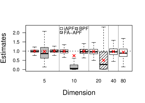
For all the simulations we ran an iAPF with $N_{0}=1000$ starting particles, a BPF with $N=10000$ particles and an FA-APF with $N=5000$ particles. The BPF and FA-APF both had slightly larger average computational times than the iAPF with these configurations. The average number of particles for the final iteration of the iAPF was greater than $N_{0}$ only in dimensions $d=40$ ($1033$) and $d=80$ ($1142$). For $d>10$, it was not possible to obtain reasonable estimates with the BPF in a feasible computational time (similarly for the FA-APF for $d>20$). The standard deviation of the samples and the average resampling count across the chosen set of dimensions are reported in Tables 1–2.

Table 1: Empirical standard deviation of the quantity $\hat{Z}/Z$ using $1000$ replicates

Dimension	$5$	$10$	$20$	$40$	$80$
iAPF	$0.09$	$0.14$	$0.19$	$0.23$	$0.35$
BPF	$0.51$	$6.4$	-	-	-
FA-APF	$0.10$	$0.17$	$0.53$	-	-

Table 2: Average resampling count for the $1000$ replicates

Dimension	$5$	$10$	$20$	$40$	$80$
iAPF	$6.93$	$15.11$	$27.61$	$42.41$	$71.88$
BPF	$99$	$99$	-	-	-
FA-APF	$26.04$	$52.71$	$84.98$	-	-

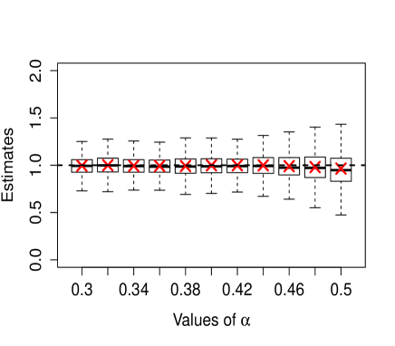
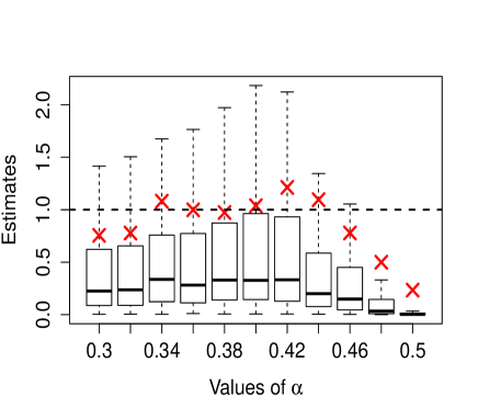
Fixing the dimension $d=10$ and the simulated sequence of observations $y_{1:T}$ with $\alpha=0.42$, we now consider the variability of the relative error of the estimates of the marginal likelihood of the observations using the iAPF and the BPF for different values of the parameter $\alpha\in\{0.3,0.32,\dots,0.48,0.5\}$. In Figure 2, we report box plots of $\hat{Z}/Z$ in $1000$ replications. For the iAPF, the length of the boxes are significantly less variable across the range of values of $\alpha$. In this case, we used $N=50000$ particles for the BPF, giving a computational time at least five times larger than that of the iAPF. This demonstrates that the approximations of the marginal likelihood $L(\alpha)$ provided by the iAPF are relatively insensitive to small changes in $\alpha$, in contrast to the BPF. Similar simulations, which we do not report, show that the FA-APF for this problem performs slightly worse than the iAPF at double the computational time.

(a) iAPF

(b) BPF

Figure 2: Box plots of $\hat{Z}/Z$ for different values of the parameter $\alpha$ using $1000$ replicates. The crosses indicate the mean of each sample.

Particle marginal Metropolis–Hastings

We consider a Linear Gaussian model with $m={\bf 0}$, $\Sigma=B=C=I_{d}$, and $D=\delta I_{d}$ with $\delta=0.25$. We used the lower-triangular matrix

$$A=\left(\begin{array}[]{ccccc}0.9&0&0&0&0\\ 0.3&0.7&0&0&0\\ 0.1&0.2&0.6&0&0\\ 0.4&0.1&0.1&0.3&0\\ 0.1&0.2&0.5&0.2&0\end{array}\right),$$

and simulated a sequence of $T=100$ observations. Assuming only that $A$ is lower triangular, for identifiability, we performed Bayesian inference for the 15 unknown parameters $\left\{A_{i,j}:i,j\in\left\{1,\dots,5\right\},j\leq i\right\}$, assigning each parameter an independent uniform prior on $[-5,5]$. From the initial point $A_{1}=I_{5}$ we ran three Markov chains $A_{1:L}^{{\rm BPF}}$, $A_{1:L}^{{\rm iAPF}}$ and $A_{1:L}^{{\rm Kalman}}$ of length $L=300000$ to explore the parameter space, updating one of the $15$ parameters components at a time with a Gaussian random walk proposal with variance $0.1$. The chains differ in how the acceptance probabilities are computed, and correspond to using unbiased estimates of the marginal likelihood obtain from the BPF, iAPF or the Kalman filter, respectively. In the latter case, this corresponds to running a Metropolis–Hastings (MH) chain by computing the marginal likelihood exactly. We started every run of the iAPF with $N_{0}=500$ particles. The resulting average number of particles used to compute the final estimate was $500.2$. The number of particles $N=20000$ for the BPF was set to have a greater computational time, in this case $A_{1:L}^{{\rm BPF}}$ took $50\%$ more time than $A_{1:L}^{{\rm iAPF}}$ to simulate.

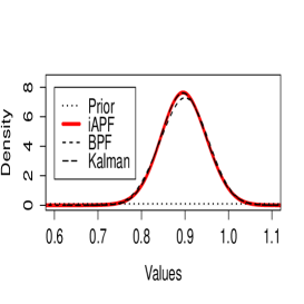
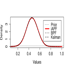
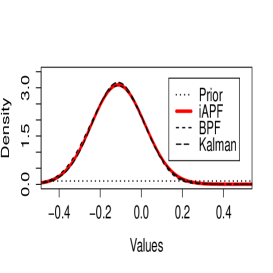
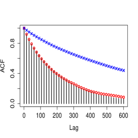
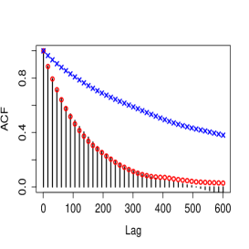
In Figure 3, we plot posterior density estimates obtained from the three chains for 3 of the 15 entries of the transition matrix $A$. The posterior means associated with the entries of the matrix $A$ were fairly close to $A$ itself, the largest discrepancy being around $0.2$, and the posterior standard deviations were all around $0.1$. A comparison of estimated Markov chain autocorrelations for these same parameters is reported in Figure 4, which indicates little difference between the iAPF-PMMH and Kalman-MH Markov chains, and substantially worse performance for the BPF-PMMH Markov chain. The integrated autocorrelation time of the Markov chains provides a measure of the asymptotic variance of the individual chains’ ergodic averages, and in this regard the iAPF-PMMH and Kalman-MH Markov chains were practically indistinguishable, while the BPF-PMMH performed between 3 and 4 times worse, depending on the parameter. The relative improvement of the iAPF over the BPF does seem empirically to depend on the value of $\delta$. In experiments with larger $\delta$, the improvement was still present but less pronounced than for $\delta=0.25$. We note that in this example, $\bm{\psi}^{*}$ is outside the class of possible $\bm{\psi}$ sequences that can be obtained using the iAPF: the approximations in $\bm{\Psi}$ are functions that are constants plus a multivariate normal density with a diagonal covariance matrix whilst the functions in $\bm{\psi}^{*}$ are multivariate normal densities whose covariance matrices have non-zero, off-diagonal entries.

(a) $A_{11}$

(b) $A_{41}$

(c) $A_{55}$

Figure 3: Linear Gaussian model: density estimates for the specified parameters from the three Markov chains.

(a) $A_{11}$

(b) $A_{41}$

(c) $A_{55}$

Figure 4: Linear Gaussian model: autocorrelation function estimates for the BPF-PMMH (crosses), iAPF-PMMH (solid lines) and Kalman-MH (circles) Markov chains.

5.3 Univariate stochastic volatility model

A simple stochastic volatility model is defined by $\mu(\cdot)=\mathcal{N}(\cdot;0,\sigma^{2}/(1-\alpha)^{2})$, $f(x,\cdot)=\mathcal{N}(\cdot;\alpha x,\sigma^{2})$ and $g(x,\cdot)=\mathcal{N}(\cdot;0,\beta^{2}\exp(x))$, where $\alpha\in(0,1)$, $\beta>0$ and $\sigma^{2}>0$ are statistical parameters (see, e.g., Kim et al., 1998). To compare the efficiency of the iAPF and the BPF within a PMMH algorithm, we analyzed a sequence of $T=945$ observations $y_{1:T}$, which are mean-corrected daily returns computed from weekday close exchange rates $r_{1:T+1}$ for the pound/dollar from 1/10/81 to 28/6/85. This data has been previously analyzed using different approaches, e.g. in Harvey et al. (1994) and Kim et al. (1998).

We wish to infer the model parameters $\theta=\left(\alpha,\sigma,\beta\right)$ using a PMMH algorithm and compare the two cases where the marginal likelihood estimates are obtained using the iAPF and the BPF. We placed independent inverse Gamma prior distributions $\mathcal{IG}\left(2.5,0.025\right)$ and $\mathcal{IG}\left(3,1\right)$ on $\sigma^{2}$ and $\beta^{2}$, respectively, and an independent ${\rm Beta}\left(20,1.5\right)$ prior distribution on the transition coefficient $\alpha$. We used $\left(\alpha_{0},\sigma_{0},\beta_{0}\right)=\left(0.95,\sqrt{0.02},0.5\right)$ as the starting point of the three chains: $X_{1:L}^{{\rm iAPF}}$, $X_{1:L}^{{\rm BPF}}$ and $X_{L^{\prime}}^{{\rm BPF}^{\prime}}$. All the chains updated one component at a time with a Gaussian random walk proposal with variances $\left(0.02,0.05,0.1\right)$ for the parameters $\left(\alpha,\sigma,\beta\right)$. $X_{1:L}^{{\rm iAPF}}$ has a total length of $L=150000$ and for the estimates of the marginal likelihood that appear in the acceptance probability we use the iAPF with $N_{0}=100$ starting particles. For $X_{1:L}^{{\rm BPF}}$ and $X_{1:L^{\prime}}^{{\rm BPF}^{\prime}}$ we use BPFs: $X_{1:L}^{{\rm BPF}^{\prime}}$ is a shorter chain with more particles ($L=150000$ and $N=1000$) while $X_{1:L^{\prime}}^{{\rm BPF}^{\prime}}$ is a longer chain with fewer particles $(L=1500000$, $N=100$). All chains required similar running time overall to simulate. Figure 5 shows estimated marginal posterior densities for the three parameters using the different chains.

(a) $\alpha$

(b) $\sigma$

(c) $\beta$

Figure 5: Stochastic Volatility model: PMMH density estimates for each parameter from the three chains.

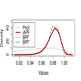
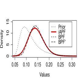
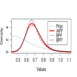
In Table 3 we provide the adjusted sample size of the Markov chains associated with each of the parameters, obtained by dividing the length of the chain by the estimated integrated autocorrelation time associated with each parameter. We can see an improvement using the iAPF, although we note that the BPF-PMMH algorithm appears to be fairly robust to the variability of the marginal likelihood estimates in this particular application.

Table 3: Sample size adjusted for autocorrelation for each parameter from the three chains.

	$\alpha$	$\sigma^{2}$	$\beta$
iAPF	3620	3952	3830
BPF	2460	2260	3271
BPF’	2470	2545	2871

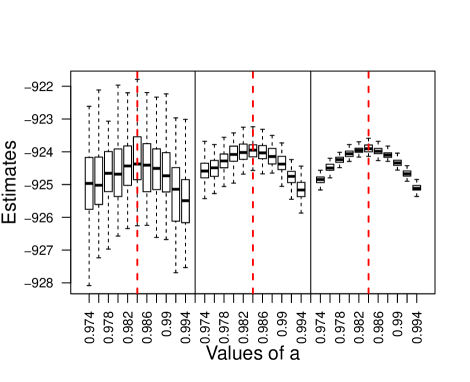
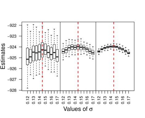
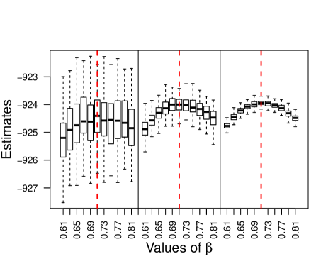
Since particle filters provide approximations of the marginal likelihood in HMMs, the iAPF can also be used in alternative parameter estimation procedures, such as simulated maximum likelihood (Lerman & Manski, 1981; Diggle & Gratton, 1984). The use of particle filters for approximate maximum likelihood estimation (see, e.g., Kitagawa, 1998; Hürzeler & Künsch, 2001) has recently been used to fit macroeconomic models (Fernández-Villaverde & Rubio-Ramírez, 2007). In Figure 6 we show the variability of the BPF and iAPF estimates of the marginal likelihood at points in a neighborhood of the approximate MLE of $(\alpha,\sigma,\beta)=(0.984,0.145,0.69)$. The iAPF with $N_{0}=100$ particles used $100$ particles in the final iteration to compute the likelihood in all simulations, and took slightly more time than the BPF with $N=1000$ particles, but far less time than the BPF with $N=10000$ particles. The results indicate that the iAPF estimates are significantly less variable than their BPF counterparts, and may therefore be more suitable in simulated maximum likelihood approximations.

(a)

(b)

(c)

Figure 6: log-likelihood estimates in a neighborhood of the MLE. Boxplots correspond to $100$ estimates at each parameter value given by three particle filters, from left to right: BPF ($N=1000$), BPF ($N=10000$), iAPF ($N_{0}=100$).

5.4 Multivariate stochastic volatility model

We consider a version of the multivariate stochastic volatility model defined for $\mathsf{X}=\mathbb{R}^{d}$ by $\mu(\cdot)=\mathcal{N}(\cdot;m,U_{\star})$, $f(x,\cdot)=\mathcal{N}(\cdot;m+{\rm diag}(\phi)\left(x-m\right),U)$ and $g(x,\cdot)=\mathcal{N}\left(\cdot;0,\exp\left({\rm diag}\left(x\right)\right)\right)$, where $m,\phi\in\mbox{$\mathbb{R}$}^{d}$ and the covariance matrix $U\in\mathbb{R}^{d\times d}$ are statistical parameters. The matrix $U_{\star}$ is the stationary covariance matrix associated with $(\phi,U)$. This is the basic MSV model in Chib et al. (2009, Section 2), with the exception that we consider a non diagonal transition covariance matrix $U$ and a diagonal observation matrix.

We analyzed two 20-dimensional sequences of observations $y_{1:T}$ and $y_{1:T^{\prime}}^{\prime}$, where $T=102$ and $T^{\prime}=90$. The sequences correspond to the monthly returns for the exchange rate with respect to the US dollar of a range of 20 different international currencies, in the periods $3/2000$–$8/2008$ ($y_{1:T}$, pre-crisis) and $9/2008$–$2/2016$ ($y_{1:T^{\prime}}^{\prime}$, post-crisis), as reported by the Federal Reserve System (available at http://www.federalreserve.gov/releases/h10/hist/). We infer the model parameters $\theta=\left(m,\phi,U\right)$ using the iAPF to obtain marginal likelihood estimates within a PMMH algorithm. A similar study using a different approach and with a set of $6$ currencies can be found in Liu & West (2001).

The aim of this study is to showcase the potential of the iAPF in a scenario where, due to the relatively high dimensionality of the state space, the BPF systematically fails to provide reasonable marginal likelihood estimates in a feasible computational time. To reduce the dimensionality of the parameter space we consider a band diagonal covariance matrix $U$ with non-zero entries on the main, upper and lower diagonals. We placed independent inverse Gamma prior distributions with mean $0.2$ and unit variance on each entry of the diagonal of $U$, and independent symmetric triangular prior distributions on $[-1,1]$ on the correlation coefficients $\rho\in\mathbb{R}^{19}$ corresponding to the upper and lower diagonal entries. We place independent Uniform$(0,1)$ prior distributions on each component of $\phi$ and an improper, constant prior density for $m$. This results in a 79-dimensional parameter space. As the starting point of the chains we used $\phi_{0}=0.95\cdot\mathbf{1}$, ${\rm diag}(U_{0})=0.2\cdot\mathbf{1}$ and for the $19$ correlation coefficients we set $\rho_{0}=0.25\cdot\mathbf{1}$, where ${\bf 1}$ denotes a vector of $1$s whose length can be determined by context. Each entry of $m_{0}$ corresponds to the logarithm of the standard deviation of the observation sequence of the relative currency.

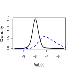
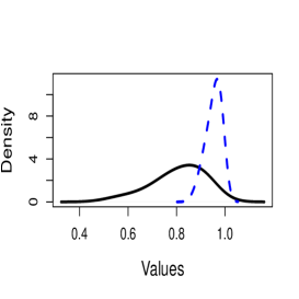
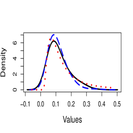
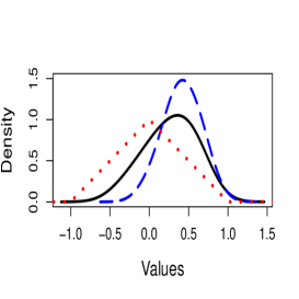
We ran two Markov chains $X_{1:L}$ and $X^{\prime}_{1:L}$, corresponding to the data sequences $y_{1:T}$ and $y_{1:T^{\prime}}^{\prime}$, both of them updated one component at a time with a Gaussian random walk proposal with standard deviations $\left(0.2\cdot\mathbf{1},0.005\cdot\mathbf{1},0.02\cdot\mbox{{1}},0.02\cdot\mathbf{1}\right)$ for the parameters $\left(m,\phi,{\rm diag}\left(U\right),\rho\right)$. The total number of updates for each parameter is $L=12000$ and the iAPF with $N_{0}=500$ starting particles is used to estimate marginal likelihoods within the PMMH algorithm. In Figure 7 we report the estimated smoothed posterior densities corresponding to the parameters for the Pound Sterling/US Dollar exchange rate series. Most of the posterior densities are different from their respective prior densities, and we also observe qualitative differences between the pre and post crisis regimes. For the same parameters, sample sizes adjusted for autocorrelation are reported in Table 4. Considering the high dimensional state and parameter spaces, these are satisfactory. In the later steps of the PMMH chain, we recorded an average number of iterations for the iAPF of around $5$ and an average number of particles in the final $\bm{\psi}$-APF of around $502$.

Table 4: Sample size adjusted for autocorrelation.

	$m_{\text{\pounds}}$	$\phi_{\text{\pounds}}$	$U_{\text{\pounds}}$	$U_{\text{\pounds,€}}$
pre-crisis	408	112	218	116
post-crisis	175	129	197	120

(a) $m_{\text{\pounds}}$

(b) $\phi_{\text{\pounds}}$

(c) $U_{\text{\pounds}}$

(d) $U_{\text{\pounds,€}}$

Figure 7: Multivariate stochastic volatility model: density estimates for the parameters related to the Pound Sterling. Pre-crisis chain (solid line), post-crisis chain (dashed line) and prior density (dotted line). The prior densities for (a) and (b) are constant.

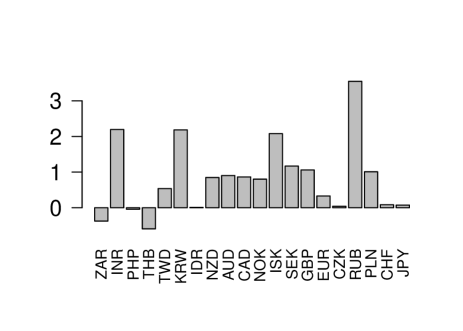
The aforementioned qualitative change of regime seems to be evident looking at the difference between the posterior expectations of the parameter $m$ for the post-crisis and the pre-crisis chain, reported in Figure 8. The parameter $m$ can be interpreted as the period average of the mean-reverting latent process of the log-volatilities for the exchange rate series. Positive values of the differences for close to all of the currencies suggest a generally higher volatility during the post-crisis period.

Figure 8: Multivariate stochastic volatility model: differences between post-crisis and pre-crisis posterior expectation of the parameter $m$ for the 20 currencies.

6 Discussion

In this article we have presented the iAPF, an offline algorithm that approximates an idealized particle filter whose marginal likelihood estimates have zero variance. The main idea is to iteratively approximate a particular sequence of functions, and an empirical study with an implementation using parametric optimization for models with Gaussian transitions showed reasonable performance in some regimes for which the BPF was not able to provide adequate approximations. We applied the iAPF to Bayesian parameter estimation in general state space HMMs by using it as an ingredient in a PMMH Markov chain. It could also conceivably be used in similar, but inexact, noisy Markov chains; Medina-Aguayo et al. (2015) showed that control on the quality of the marginal likelihood estimates can provide theoretical guarantees on the behaviour of the noisy Markov chain. The performance of the iAPF marginal likelihood estimates also suggests they may be useful in simulated maximum likelihood procedures. In our empirical studies, the number of particles used by the iAPF was orders of magnitude smaller than would be required by the BPF for similar approximation accuracy, which may be relevant for models in which space complexity is an issue.

In the context of likelihood estimation, the perspective brought by viewing the design of particle filters as essentially a function approximation problem has the potential to significantly improve the performance of such methods in a variety of settings. There are, however, a number of alternatives to the parametric optimization approach described in Section 5.1, and it would be of particular future interest to investigate more sophisticated schemes for estimating $\bm{\psi}^{*}$, i.e. specific implementations of Algorithm 3. We have used nonparametric estimates of the sequence $\bm{\psi}^{*}$ with some success, but the computational cost of the approach was much larger than the parametric approach. Alternatives to the classes $\mathcal{F}$ and $\Psi$ described in Section 3.2 could be obtained using other conjugate families, (see, e.g., Vidoni, 1999). We also note that although we restricted the matrix $\Sigma$ in (15) to be diagonal in our examples, the resulting iAPF marginal likelihood estimators performed fairly well in some situations where the optimal sequence $\bm{\psi}^{*}$ contained functions that could not be perfectly approximated using any function in the corresponding class. Finally, the stopping rule in the iAPF, described in Algorithm 4 and which requires multiple independent marginal likelihood estimates, could be replaced with a stopping rule based on the variance estimators proposed in Lee & Whiteley (2015). For simplicity, we have discussed particle filters in which multinomial resampling is used; a variety of other resampling strategies (see Douc et al., 2005, for a review) can be used instead.

Appendix A Expression for the asymptotic variance in the CLT

Proof of Proposition 3.

We define a sequence of densities by

$$\pi_{k}^{\bm{\psi}}(x_{1:T}):=\frac{\left[\mu_{1}^{\bm{\psi}}\left(x_{1}\right)\prod_{t=2}^{T}f_{t}^{\bm{\psi}}\left(x_{t-1},x_{t}\right)\right]\prod_{t=1}^{k}g_{t}^{\bm{\psi}}\left(x_{t}\right)}{\int_{\mathsf{X}^{T}}\left[\mu_{1}^{\bm{\psi}}\left(x_{1}\right)\prod_{t=2}^{T}f_{t}^{\bm{\psi}}\left(x_{t-1},x_{t}\right)\right]\prod_{t=1}^{k}g_{t}^{\bm{\psi}}\left(x_{t}\right)dx_{1:T}},\quad x_{1:T}\in\mathsf{X}^{T},$$

for each $k\in\{1,\ldots,T\}$. We also define $\pi_{k}^{\bm{\psi}}(x_{j}):=\int\pi_{k}(x_{1:j-1},x_{j},x_{j+1:T})dx_{-j}$ for $j\in\{1,\ldots,T\}$, where $x_{-j}:=(x_{1},\ldots,x_{j-1},x_{j+1},\ldots,x_{N})$. Combining equation $(24.37)$ of Doucet & Johansen (2011) with elementary manipulations provides,

$$\sigma_{\bm{\psi}}^{2} = \sum_{t=1}^{T}\left[\int_{\mathsf{X}}\frac{\pi_{T}^{\bm{\psi}}(x_{t})^{2}}{\pi_{t-1}^{\bm{\psi}}(x_{t})}dx_{t}-1\right]$$

$$= \sum_{t=1}^{T}\left[\int_{\mathsf{X}}\frac{\psi_{t}^{*}(x_{t})}{\psi_{t}(x_{t})}\pi_{T}^{\bm{\psi}}(x_{t})dx_{t}\cdot\frac{\int_{\mathsf{X}}\psi_{t}\left(x_{t}\right)\pi_{t-1}^{\bm{\psi}}(x_{t})dx_{t}}{\int_{\mathsf{X}}\psi_{t}^{*}\left(x_{t}\right)\pi_{t-1}^{\bm{\psi}}(x_{t})dx_{t}}-1\right]$$

$$= \sum_{t=1}^{T}\left\{\mathbb{E}\left[\frac{\psi_{t}^{*}\left(X_{t}\right)}{\psi_{t}\left(X_{t}\right)}\Bigl{|}\left\{Y_{1:T}=y_{1:T}\right\}\right]\frac{\mathbb{E}\left[\psi_{t}\left(X_{t}\right)\mid\left\{Y_{1:t-1}=y_{1:t-1}\right\}\right]}{\mathbb{E}\left[\psi_{t}^{*}\left(X_{t}\right)\mid\left\{Y_{1:t-1}=y_{1:t-1}\right\}\right]}-1\right\},$$

and the expression involving the rescaled terms $\bar{\psi}_{t}^{*}$ and $\bar{\psi}_{t}$ then follows. ∎

References

- (1)
- Andrieu et al. (2010) Andrieu, C., Doucet, A. & Holenstein, R. (2010), ‘Particle Markov chain Monte Carlo methods’, Journal of the Royal Statistical Society: Series B (Statistical Methodology) 72(3), 269–342.
- Andrieu & Roberts (2009) Andrieu, C. & Roberts, G. O. (2009), ‘The Pseudo-Marginal approach for efficient Monte Carlo computations’, The Annals of Statistics pp. 697–725.
- Andrieu & Vihola (2015) Andrieu, C. & Vihola, M. (2015), ‘Convergence properties of pseudo-marginal Markov chain Monte Carlo algorithms’, The Annals of Applied Probability 25(2), 1030–1077.
- Beaumont (2003) Beaumont, M. A. (2003), ‘Estimation of population growth or decline in genetically monitored populations’, Genetics 164(3), 1139–1160.
- Bérard et al. (2014) Bérard, J., Del Moral, P. & Doucet, A. (2014), ‘A lognormal central limit theorem for particle approximations of normalizing constants’, Electronic Journal of Probability 19(94), 1–28.
- Chen et al. (2000) Chen, R., Wang, X. & Liu, J. S. (2000), ‘Adaptive joint detection and decoding in flat-fading channels via mixture Kalman filtering’, Information Theory, IEEE Transactions on 46(6), 2079–2094.
- Chib et al. (2009) Chib, S., Omori, Y. & Asai, M. (2009), Multivariate stochastic volatility, in T. G. Andersen, R. A. Davis, J.-P. Kreiss & T. V. Mikosch, eds, ‘Handbook of Financial Time Series’, Springer, pp. 365–400.
- Chopin (2004) Chopin, N. (2004), ‘Central limit theorem for sequential Monte Carlo methods and its application to Bayesian inference’, The Annals of Statistics pp. 2385–2411.
- Clapp & Godsill (1999) Clapp, T. C. & Godsill, S. J. (1999), ‘Fixed-lag smoothing using sequential importance sampling’, Bayesian Statistics 6: Proceedings of the Sixth Valencia International Meeting 6, 743–752.
- Del Moral (2004) Del Moral, P. (2004), Feynman-Kac Formulae, Springer.
- Del Moral & Guionnet (1999) Del Moral, P. & Guionnet, A. (1999), ‘Central limit theorem for nonlinear filtering and interacting particle systems’, The Annals of Applied Probability 9(2), 275–297.
- Diggle & Gratton (1984) Diggle, P. J. & Gratton, R. J. (1984), ‘Monte Carlo methods of inference for implicit statistical models’, Journal of the Royal Statistical Society. Series B (Methodological) pp. 193–227.
- Douc et al. (2005) Douc, R., Cappé, O. & Moulines, E. (2005), Comparison of resampling schemes for particle filtering, in ‘Image and Signal Processing and Analysis, 2005. ISPA 2005. Proceedings of the 4th International Symposium on’, IEEE, pp. 64–69.
- Douc & Moulines (2008) Douc, R. & Moulines, E. (2008), ‘Limit theorems for weighted samples with applications to sequential Monte Carlo methods’, The Annals of Statistics 36(5), 2344–2376.
- Doucet et al. (2006) Doucet, A., Briers, M. & Sénécal, S. (2006), ‘Efficient block sampling strategies for sequential Monte Carlo methods’, Journal of Computational and Graphical Statistics 15(3).
- Doucet et al. (2000) Doucet, A., Godsill, S. & Andrieu, C. (2000), ‘On sequential Monte Carlo sampling methods for Bayesian filtering’, Statistics and Computing 10(3), 197–208.
- Doucet & Johansen (2011) Doucet, A. & Johansen, A. M. (2011), A tutorial on particle filtering and smoothing: Fiteen years later, in D. Crisan & B. Rozovsky, eds, ‘The Oxford Handbook of Nonlinear Filtering’, pp. 656–704.
- Doucet et al. (2015) Doucet, A., Pitt, M., Deligiannidis, G. & Kohn, R. (2015), ‘Efficient implementation of Markov chain Monte Carlo when using an unbiased likelihood estimator’, Biometrika 102(2), 295–313.
- Fernández-Villaverde & Rubio-Ramírez (2007) Fernández-Villaverde, J. & Rubio-Ramírez, J. F. (2007), ‘Estimating macroeconomic models: A likelihood approach’, The Review of Economic Studies 74(4), 1059–1087.
- Gordon et al. (1993) Gordon, N. J., Salmond, D. J. & Smith, A. F. (1993), ‘Novel approach to nonlinear/non-Gaussian Bayesian state estimation’, IEE Proceedings-Radar, Sonar and Navigation 140(2), 107–113.
- Harvey et al. (1994) Harvey, A., Ruiz, E. & Shephard, N. (1994), ‘Multivariate stochastic variance models’, The Review of Economic Studies 61(2), 247–264.
- Hürzeler & Künsch (2001) Hürzeler, M. & Künsch, H. R. (2001), Approximating and maximising the likelihood for a general state-space model, in A. Doucet, N. de Freitas & N. Gordon, eds, ‘Sequential Monte Carlo methods in practice’, Springer, pp. 159–175.
- Johansen & Doucet (2008) Johansen, A. M. & Doucet, A. (2008), ‘A note on auxiliary particle filters’, Statistics & Probability Letters 78(12), 1498–1504.
- Kim et al. (1998) Kim, S., Shephard, N. & Chib, S. (1998), ‘Stochastic volatility: likelihood inference and comparison with arch models’, The Review of Economic Studies 65(3), 361–393.
- Kitagawa (1998) Kitagawa, G. (1998), ‘A self-organizing state-space model’, Journal of the American Statistical Association pp. 1203–1215.
- Kong et al. (1994) Kong, A., Liu, J. S. & Wong, W. H. (1994), ‘Sequential imputations and Bayesian missing data problems’, Journal of the American Statistical Association 89(425), 278–288.
- Künsch (2005) Künsch, H. (2005), ‘Recursive Monte Carlo filters: algorithms and theoretical analysis’, The Annals of Statistics 33(5), 1983–2021.
- Lee & Łatuszyński (2014) Lee, A. & Łatuszyński, K. (2014), ‘Variance bounding and geometric ergodicity of Markov chain Monte Carlo kernels for approximate Bayesian computation.’, Biometrika 101(3), 655–671.
- Lee & Whiteley (2015) Lee, A. & Whiteley, N. (2015), ‘Variance estimation and allocation in the particle filter’, arXiv preprint arXiv:1509.00394 .
- Lerman & Manski (1981) Lerman, S. & Manski, C. (1981), On the use of simulated frequencies to approximate choice probabilities, in ‘Structural analysis of discrete data with econometric applications’, The MIT press, pp. 305–319.
- Lin et al. (2013) Lin, M., Chen, R., Liu, J. S. et al. (2013), ‘Lookahead strategies for sequential Monte Carlo’, Statistical Science 28(1), 69–94.
- Liu & Chen (1995) Liu, J. S. & Chen, R. (1995), ‘Blind deconvolution via sequential imputations’, Journal of the American Statistical Association 90, 567–576.
- Liu & West (2001) Liu, J. & West, M. (2001), Combined parameter and state estimation in simulation-based filtering, in A. Doucet, N. de Freitas & N. Gordon, eds, ‘Sequential Monte Carlo methods in practice’, Springer, pp. 197–223.
- Medina-Aguayo et al. (2015) Medina-Aguayo, F. J., Lee, A. & Roberts, G. O. (2015), ‘Stability of noisy Metropolis–Hastings’, arXiv preprint arXiv:1503.07066 .
- Nadaraya (1964) Nadaraya, E. A. (1964), ‘On estimating regression’, Theory of Probability & Its Applications 9(1), 141–142.
- Pitt & Shephard (1999) Pitt, M. K. & Shephard, N. (1999), ‘Filtering via simulation: Auxiliary particle filters’, Journal of the American Statistical Association 94(446), 590–599.
- Sherlock et al. (2015) Sherlock, C., Thiery, A. H., Roberts, G. O. & Rosenthal, J. S. (2015), ‘On the efficiency of pseudo-marginal random walk Metropolis algorithms’, The Annals of Statistics 43(1), 238–275.
- Vidoni (1999) Vidoni, P. (1999), ‘Exponential family state space models based on a conjugate latent process’, Journal of the Royal Statistical Society: Series B (Statistical Methodology) 61(1), 213–221.
- Walker (1974) Walker, A. J. (1974), ‘New fast method for generating discrete random numbers with arbitrary frequency distributions’, Electronics Letters 10(8), 127–128.
- Walker (1977) Walker, A. J. (1977), ‘An efficient method for generating discrete random variables with general distributions’, ACM Transactions on Mathematical Software 3(3), 253–256.
- Watson (1964) Watson, G. S. (1964), ‘Smooth regression analysis’, Sankhyā: The Indian Journal of Statistics, Series A 26(4), 359–372.
- Whiteley & Lee (2014) Whiteley, N. & Lee, A. (2014), ‘Twisted particle filters’, The Annals of Statistics 42(1), 115–141.