Declutter and Resample: Towards parameter free denoising

Abstract

In many data analysis applications the following scenario is commonplace: we are given a point set that is supposed to sample a hidden ground truth $K$ in a metric space, but it got corrupted with noise so that some of the data points lie far away from $K$ creating outliers also termed as ambient noise. One of the main goals of denoising algorithms is to eliminate such noise so that the curated data lie within a bounded Hausdorff distance of $K$. Popular denoising approaches such as deconvolution and thresholding often require the user to set several parameters and/or to choose an appropriate noise model while guaranteeing only asymptotic convergence. Our goal is to lighten this burden as much as possible while ensuring theoretical guarantees in all cases.

Specifically, first, we propose a simple denoising algorithm that requires only a single parameter but provides a theoretical guarantee on the quality of the output on general input points. We argue that this single parameter cannot be avoided. We next present a simple algorithm that avoids even this parameter by paying for it with a slight strengthening of the sampling condition on the input points which is not unrealistic. We also provide some preliminary empirical evidence that our algorithms are effective in practice.

1 Introduction

Real life data are almost always corrupted by noise. Of course, when we talk about noise, we implicitly assume that the data sample a hidden space called the ground truth with respect to which we measure the extent and type of noise. Some data can lie far away from the ground truth leading to ambient noise. Clearly, the data density needs to be higher near the ground truth if signal has to prevail over noise. Therefore, a worthwhile goal of a denoising algorithm is to curate the data, eliminating the ambient noise while retaining most of the subset that lies within a bounded distance from the ground truth.

In this paper we are interested in removing “outlier”-type of noise from input data. Numerous algorithms have been developed for this problem in many different application fields; see e.g [21, 27]. There are two popular families of denoising/outlier detection approaches: Deconvolution and Thresholding. Deconvolution methods rely on the knowledge of a generative noise model for the data. For example, the algorithm may assume that the input data has been sampled according to a probability measure obtained by convolving a distribution such as a Gaussian [23] with a measure whose support is the ground truth. Alternatively, it may assume that the data is generated according to a probability measure with a small Wasserstein distance to a measure supported by the ground truth [7]. The denoising algorithm attempts to cancel the noise by deconvolving the data with the assumed model.

A deconvolution algorithm requires the knowledge of the generative model and at least a bound on the parameter(s) involved, such as the standard deviation of the Gaussian convolution or the Wasserstein distance. Therefore, it requires at least one parameter as well as the knowledge of the noise type. The results obtained in this setting are often asymptotic, that is, theoretical guarantees hold in the limit when the number of points tends to infinity.

The method of thresholding relies on a density estimation procedure [26] by which it estimates the density of the input locally. The data is cleaned, either by removing points where density is lower than a threshold [16], or moving them from such areas toward higher densities using gradient-like methods such as mean-shift [13, 25]. It has been recently used for uncovering geometric information such as one dimensional features [18]. In [5], the distance to a measure [10] that can also be seen as a density estimator [2] has been exploited for thresholding. Other than selecting a threshold, these methods require the choice of a density estimator. This estimation requires at least one additional parameter, either to define a kernel, or a mass to define the distance to a measure. In the case of a gradient based movement of the points, the nature of the movement also has to be defined by fixing the length of a step and by determining the terminating condition of the algorithm.

New work.  In above classical methods, the user is burdened with making several choices such as fixing an appropriate noise model, selecting a threshold and/or other parameters. Our main goal is to lighten this burden as much as possible. First, we show that denoising with a single parameter is possible and this parameter is in some sense unavoidable unless a stronger sampling condition on the input points is assumed. This leads to our main algorithm that is completely free of any parameter when the input satisfies a stronger sampling condition which is not unrealistic.

Our first algorithm Declutter algorithm uses a single parameter (presented in Section 3) and assumes a very general sampling condition which is not stricter than those for the classical noise models mentioned previously because it holds with high probability for those models as well. Additionally, our sampling condition also allows ambient noise and locally adaptive samplings. Interestingly, we note that our Declutter algorithm is in fact a variant of the approach proposed in [8] to construct the so-called $\varepsilon$-density net. Indeed, as we point out in Appendix D , the procedure of [8] can also be directly used for denoising purpose and one can obtain an analog of Theorems 3.3 and 3.7 in this paper for the resulting density net.

Figure 1: From left to right: the input sample,the output of Algorithm Declutter when $k=2$, the output of Algorithm Declutter when $k=10$,the output of Algorithm ParfreeDeclutter.

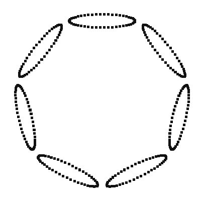
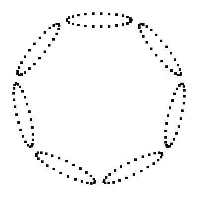
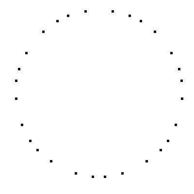
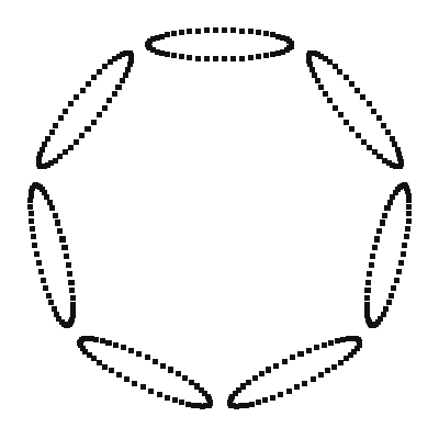
Use of a parameter in the denoising process is unavoidable in some sense, unless there are other assumptions about the hidden space. This is illustrated by the example in Figure 1. Does the sample here represent a set of small loops or one big circle? The answer depends on the scale at which we examine the data. The choice of a parameter may represent this choice of the scale [3, 15]. To remove this parameter, one needs other conditions for either the hidden space itself or for the sample, say by assuming that the data has some uniformity. Aiming to keep the sampling restrictions as minimal as possible, we show that it is sufficient to assume the homogeneity in data only on or close to the ground truth for our second algorithm which requires no input parameter.

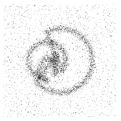
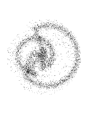
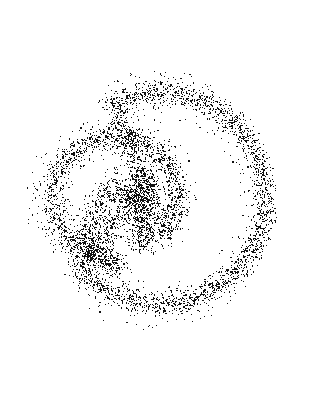
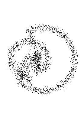
Specifically, the parameter-free algorithm presented in Section 4 relies on an iteration that intertwines our decluttering algorithm with a novel resampling procedure. Assuming that the sample is sufficiently dense and somewhat uniform near the ground truth at scales beyond a particular scale $s$, our algorithm selects a subset of the input point set that is close to the ground truth without requiring any input from the user. The output maintains the quality at scale $s$ even though the algorithm has no explicit knowledge of this parameter. See Figure 2 for an example.

Figure 2: From left to right: the ground truth, the noisy input samples ($\sim 7000$ points around the ground truth and 2000 ambient noise points), two intermediate steps of our iterative parameter-free denoising algorithm and the final output.

All missing details from this extended abstract can be found in the appendix. In addition, in Appendix C, we show how the denoised data set can be used for homology inference. In Appendix E, we provide various preliminary experimental results of our denoising algorithms.

Remark.  Very recently, Jiang and Kpotufe proposed a consistent algorithm for estimating the so-called modal-sets with also only one parameter [22]. The problem setup and goals are very different: In their work, they assume that input points are sampled from a density field that is locally maximal and constant on a compact domain. The goal is to show that as the number of samples $n$ tends to infinity, such domains (referred to as modal-sets in their paper) can be recovered, and the recovered set converges to the true modal-sets under the Hausdorff distance. We also note that our Declutter algorithm allows adaptive sampling as well.

2 Preliminaries

We assume that the input is a set of points $P$ sampled around a hidden compact set $K$, the ground truth, in a metric space $(\mathbb{X},d_{\mathbb{X}})$. For simplicity, in what follows the reader can assume $\mathbb{X}=\mathbb{R}^{d}$ with $P,K\subset\mathbb{X}=\mathbb{R}^{d}$, and the metric $d_{\mathbb{X}}$ of $\mathbb{X}$ is simply the Euclidean distance. Our goal is to process $P$ into another point set $Q$ guaranteed to be Hausdorff close to $K$ and hence to be a better sample of the hidden space $K$ for further applications. By Hausdorff close, we mean that the (standard) Hausdorff distance $\delta_{H}(Q,K)$ between $Q$ and $K$, defined as the infimum of $\delta$ such that $\forall p\in Q,d_{\mathbb{X}}(p,K)\leq\delta$ and $\forall x\in K,d_{\mathbb{X}}(x,Q)\leq\delta$, is bounded. Note that ambient noise/outliers can incur a very large Hausdorff distance.

The quality of the output point set $Q$ obviously depends on the “quality” of input points $P$, which we formalize via the language of sampling conditions. We wish to produce good quality output for inputs satisfying much weaker sampling conditions than a bounded Hausdorff distance. Our sampling condition is based on the sampling condition introduced and studied in [4, 5]; see Chapter 6 of [4] for discussions on the relation of their sampling condition with some of the common noise models such as Gaussian. Below, we first introduce a basic sampling condition deduced from the one in [4, 5], and then introduce its extensions incorporating adaptivity and uniformity.

Basic sampling condition.  Our sampling condition is built upon the concept of $k$-distance, which is a specific instance of a broader concept called distance to a measure introduced in [10]. The $k$-distance $d_{P,k}(x)$ is simply the root mean of square distance from $x$ to its $k$-nearest neighbors in $P$. The averaging makes it robust to outliers. One can view $d_{P,k}(x)$ as capturing the inverse of the density of points in $P$ around $x$ [2]. As we show in Appendix D, this specific form of $k$-distance is not essential – Indeed, several of its variants can replace its role in the definition of sampling conditions below, and our Declutter algorithm will achieve similar denoising guarantees.

Definition 2.1 ([10]).

Given a point $x\in\mathbb{X}$, let $p_{i}(x)\in P$ denote the $i$-th nearest neighbor of $x$ in $P$. The $k$-distance to a point set $P\subseteq\mathbb{X}$ is $d_{P,k}(x)=\sqrt{\frac{1}{k}\sum_{i=1}^{k}d_{\mathbb{X}}(x,p_{i}(x))^{2}}$.

Claim 2.2 ([10]).

$d_{P,k}(\cdot)$ is 1-Lipschitz, i.e. $|d_{P,k}(x)-d_{P,k}(y)|\leq d_{\mathbb{X}}(x,y)$ for $\forall(x,y)\in\mathbb{X}\times\mathbb{X}$.

All our sampling conditions are dependent on the choice of $k$ in the $k$-distance, which we reflect by writing $\epsilon_{k}$ instead of $\epsilon$ in the sampling conditions below. The following definition is related to the sampling condition proposed in [5].

Definition 2.3.

Given a compact set $K\subseteq\mathbb{X}$ and a parameter $k$, a point set $P$ is an $\epsilon_{k}$-noisy sample of $K$ if

1. $\forall x\in K,\ d_{P,k}(x)\leq\epsilon_{k}$

2. $\forall x\in\mathbb{X},\ d_{\mathbb{X}}(x,K)\leq d_{P,k}(x)+\epsilon_{k}$

Condition $1$ in Definition 2.3 means that the density of $P$ on the compact set $K$ is bounded from below, that is, $K$ is well-sampled by $P$. Note, we only require $P$ to be a dense enough sample of $K$ – there is no uniformity requirement in the sampling here.

Condition $2$ implies that a point with low $k$-distance, i.e. lying in high density region, has to be close to $K$. Intuitively, $P$ can contain outliers which can form small clusters but their density can not be significant compared to the density of points near the compact set $K$.

Note that the choice of $\epsilon_{k}$ always exists for a bounded point set $P$, no matter what value of $k$ is – For example, one can set $\epsilon_{k}$ to be the diameter of point set $P$. However, the smallest possible choice of $\epsilon_{k}$ to make $P$ an $\epsilon_{k}$-noisy sample of $K$ depends on the value of $k$. We thus use $\epsilon_{k}$ in the sampling condition to reflect this dependency.

In Section 4, we develop a parameter-free denoising algorithm. As Figure 1 illustrates, it is necessary to have a mechanism to remove potential ambiguity about the ground truth. We do so by using a stronger sampling condition to enforce some degree of uniformity:

Definition 2.4.

Given a compact set $K\subseteq\mathbb{X}$ and a parameter $k$, a point set $P$ is a uniform $(\epsilon_{k},c)$-noisy sample of $K$ if $P$ is an $\epsilon_{k}$-noisy sample of $K$ (i.e, conditions of Def. 2.3 hold) and

1. $\forall p\in P,\ d_{P,k}(p)\geq\frac{\epsilon_{k}}{c}.$

It is important to note that the lower bound in Condition $3$ enforces that the sampling needs to be homogeneous – i.e, $d_{P,k}(x)$ is bounded both from above and from below by some constant factor of $\epsilon_{k}$ – only for points on and around the ground truth $K$. This is because condition $1$ in Def. 2.3 is only for points from $K$, and condition 1 together with the $1$-Lipschitz property of $d_{P,k}$ (Claim 2.2) leads to an upper bound of $O(\epsilon_{k})$ for $d_{P,k}(y)$ only for points $y$ within $O(\epsilon_{k})$ distance to $K$. There is no such upper bound on $d_{P,k}$ for noisy points far away from $K$ and thus no homogeneity/uniformity requirements for them.

Adaptive sampling conditions.  The sampling conditions given above are global, meaning that they do not respect the “features” of the ground truth. We now introduce an adaptive version of the sampling conditions with respect to a feature size function.

Definition 2.5.

Given a compact set $K\subseteq\mathbb{X}$, a feature size function $f:K\rightarrow\mathbb{R}^{+}\cup\{0\}$ is a $1$-Lipschitz non-negative real function on $K$.

Several feature sizes exist in the literature of manifold reconstruction and topology inference, including the local feature size [1], local weak feature size, $\mu$-local weak feature size [9] or lean set feature size [14]. All of these functions describe how complicated a compact set is locally, and therefore indicate how dense a sample should be locally so that information can be inferred faithfully. Any of these functions can be used as a feature size function to define the adaptive sampling below. Let $\bar{p}$ denote any one of the nearest points of $p$ in $K$. Observe that, in general, a point $p$ can have multiple such nearest points.

Definition 2.6.

Given a compact set $K\subseteq\mathbb{X}$, a feature size function $f$ of $K$, and a parameter $k$, a point set $P$ is a uniform $(\epsilon_{k},c)$-adaptive noisy sample of $K$ if

1. $\forall x\in K,\ d_{P,k}(x)\leq\epsilon_{k}f(x)$.

2. $\forall y\in\mathbb{X},\ d_{\mathbb{X}}(y,K)\leq d_{P,k}(y)+\epsilon_{k}f(\bar{y})$.

3. $\forall p\in P,\ d_{P,k}(p)\geq\frac{\epsilon_{k}}{c}f(\bar{p})$.

We say that $P$ is an $\epsilon_{k}$-adaptive noisy sample of $K$ if only conditions 1 and 2 above hold.

We require that the feature size is positive everywhere as otherwise, the sampling condition may require infinite samples in some cases. We also note that the requirement of the feature size function being 1-Lipschitz is only needed to provide the theoretical guarantee for our second parameter-free algorithm.

3 Decluttering

We now present a simple yet effective denoising algorithm which takes as input a set of points $P$ and a parameter $k$, and outputs a set of points $Q\subseteq P$ with the following guarantees: If $P$ is an $\epsilon_{k}$-noisy sample of a hidden compact set $K\subseteq\mathbb{X}$, then the output $Q$ lies close to $K$ in the Hausdorff distance (i.e, within a small tubular neighborhood of $K$ and outliers are all eliminated). The theoretical guarantee holds for both the non-adaptive and the adaptive cases, as stated in Theorems 3.3 and 3.7.

Data: Point set $P$, parameter $k$

Result: Denoised point set $Q$

1 begin

2       sort P such that $d_{P,k}(p_{1})\leq\dots\leq d_{P,k}(p_{|P|})$.

3      

4      $Q_{0}\longleftarrow\emptyset$

5      

6      for $i\longleftarrow 1$ to $|P|$ do

7             if $Q_{i-1}\cap B(p_{i},2d_{P,k}(p_{i}))=\emptyset$ then

8                  $Q_{i}=Q_{i-1}\cup\{p_{i}\}$

9            else   $Q_{i}=Q_{i-1}$

10      $Q\longleftarrow Q_{n}$

11      

12

Algorithm 1 Declutter($P$,$k$)

As the $k$-distance behaves like the inverse of density, points with a low $k$-distance are expected to lie close to the ground truth $K$. A possible approach is to fix a threshold $\alpha$ and only keep the points with a $k$-distance less than $\alpha$. This thresholding solution requires an additional parameter $\alpha$. Furthermore, very importantly, such a thresholding approach does not easily work for adaptive samples, where the density in an area with large feature size can be lower than the density of noise close to an area with small feature size.

Our algorithm Declutter($P$,$k$), presented in Algorithm 1, works around these problems by considering the points in the order of increasing values of their $k$-distances and using a pruning step: Given a point $p_{i}$, if there exists a point $q$ deemed better in its vicinity, i.e., $q$ has smaller $k$-distance and has been previously selected $(q\in Q_{i-1})$, then $p_{i}$ is not necessary to describe the ground truth and we throw it away. Conversely, if no point close to $p_{i}$ has already been selected, then $p_{i}$ is meaningful and we keep it. The notion of “closeness” or “vicinity” is defined using the $k$-distance, so $k$ is the only parameter. In particular, the “vicinity” of a point $p_{i}$ is defined as the metric ball $B(p_{i},2d_{P,k}(p_{i}))$; observe that this radius is different for different points, and the radius of the ball is larger for outliers. Intuitively, the radius $2d_{P,k}(p_{i})$ of the “vicinity” around $p_{i}$ can be viewed as the length we have to go over to reach the hidden domain with certainty. So, bad points have a larger “vicinity”. We remark that this process is related to the construction of the “density net” introduced in [8], which we discuss more in Appendix D .

Figure 3: Declutter.

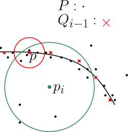
See Figure 3 on the right for an artificial example, where the black points are input points, and red crosses are in the current output $Q_{i-1}$. Now, at the $i$th iteration, suppose we are processing the point $p_{i}$ (the green point). Since within the vicinity of $p_{i}$ there is already a good point $p$, we consider $p_{i}$ to be not useful, and remove it. Intuitively, for an outlier $p_{i}$, it has a large $k$-distance and hence a large vicinity. As we show later, our $\epsilon_{k}$-noisy sampling condition ensures that this vicinity of $p_{i}$ reaches the hidden compact set which the input points presumably sample. Since points around the hidden compact set should have higher density, there should be a good point already chosen in $Q_{i-1}$. Finally, it is also important to note that, contrary to many common sparsification procedures, our Declutter algorithm removes a noisy point because it has a good point within its vicinity, and not because it is within the vicinity of a good point. For example, in Figure 3, the red points such as $p$ have small vicinity, and $p_{i}$ is not in the vicinity of any of the red point.

In what follows, we will make this intuition more concrete. We first consider the simpler non-adaptive case where $P$ is an $\epsilon_{k}$-noisy sample of $K$. We establish that $Q$ and the ground truth $K$ are Hausdorff close in the following two lemmas. The first lemma says that the ground truth $K$ is well-sampled (w.r.t. $\epsilon_{k}$) by the output $Q$ of Declutter.

Lemma 3.1.

Let $Q\subseteq P$ be the output of Declutter($P$,$k$) where $P$ is an $\epsilon_{k}$-noisy sample of a compact set $K\subseteq\mathbb{X}$. Then, for any $x\in K$, there exists $q\in Q$ such that $d_{\mathbb{X}}(x,q)\leq 5\epsilon_{k}$.

Proof.

Let $x\in K$. By Condition 1 of Def. 2.3, we have $d_{P,k}(x)\leq\epsilon_{k}$. This means that the nearest neighbor $p_{i}$ of $x$ in $P$ satisfies $d_{\mathbb{X}}(p_{i},x)\leq d_{P,k}(x)\leq\epsilon_{k}$. If $p_{i}\in Q$, then the claim holds by setting $q=p_{i}$. If $p_{i}\notin Q$, there must exist $j<i$ with $p_{j}\in Q_{i-1}$ such that $d_{\mathbb{X}}(p_{i},p_{j})\leq 2d_{P,k}(p_{i})$. In other words, $p_{i}$ was removed by our algorithm because $p_{j}\in Q_{i-1}\cap B(p_{i},2d_{P,k}(p_{i}))$. Combining triangle inequality with the 1-Lipschitz property of $d_{P,k}$ (Claim 2.2), we then have

$$d_{\mathbb{X}}(x,p_{j})\leq d_{\mathbb{X}}(x,p_{i})+d_{\mathbb{X}}(p_{i},p_{j})\leq d_{\mathbb{X}}(x,p_{i})+2d_{P,k}(p_{i})\leq 2d_{P,k}(x)+3d_{\mathbb{X}}(p_{i},x)\leq 5\epsilon_{k},$$

which proves the claim. ∎

The next lemma implies that all outliers are removed by our denoising algorithm.

Lemma 3.2.

Let $Q\subseteq P$ be the output of Declutter($P$,$k$) where $P$ is an $\epsilon_{k}$-noisy sample of a compact set $K\subseteq\mathbb{X}$. Then, for any $q\in Q$, there exists $x\in K$ such that $d_{\mathbb{X}}(q,x)\leq 7\epsilon_{k}.$

Proof.

Consider any $p_{i}\in P$ and let $\bar{p}_{i}$ be one of its nearest points in $K$. It is sufficient to show that if $d_{\mathbb{X}}(p_{i},\bar{p}_{i})>7\epsilon_{k}$, then $p_{i}\notin Q$ .

Indeed, by Condition 2 of Def. 2.3, $d_{P,k}(p_{i})\geq d_{\mathbb{X}}(p_{i},\bar{p}_{i})-\epsilon_{k}>6\epsilon_{k}$. By Lemma 3.1, there exists $q\in Q$ such that $d_{\mathbb{X}}(\bar{p}_{i},q)\leq 5\epsilon_{k}$. Thus,

$$d_{P,k}(q)\leq d_{P,k}(\bar{p}_{i})+d_{\mathbb{X}}(\bar{p}_{i},q)\leq 6\epsilon_{k}.$$

Therefore, $d_{P,k}(p_{i})>6\epsilon_{k}\geq d_{P,k}(q)$ implying that $q\in Q_{i-1}$. Combining triangle inequality and Condition 2 of Def. 2.3, we have

$$d_{\mathbb{X}}(p_{i},q)\leq d_{\mathbb{X}}(p_{i},\bar{p}_{i})+d_{\mathbb{X}}(\bar{p}_{i},q)\leq d_{P,k}(p_{i})+\epsilon_{k}+5\epsilon_{k}<2d_{P,k}(p_{i}).$$

Therefore, $q\in Q_{i-1}\cap B(p_{i},2d_{P,k}(p_{i}))$, meaning that $p_{i}\notin Q$. ∎

Theorem 3.3.

Given a point set $P$ which is an $\epsilon_{k}$-noisy sample of a compact set $K\subseteq\mathbb{X}$, Algorithm Declutter returns a set $Q\subseteq P$ such that $\delta_{H}(K,Q)\leq 7\epsilon_{k}.$

Interestingly, if the input point set is uniform then the denoised set is also uniform, a fact that turns out to be useful for our parameter-free algorithm later.

Proposition 3.4.

If $P$ is a uniform $(\epsilon_{k},c)$-noisy sample of a compact set $K\subseteq\mathbb{X}$, then the distance between any pair of points of $Q$ is at least $2\frac{\epsilon_{k}}{c}$.

Proof.

Let $p$ and $q$ be in $Q$ with $p\neq q$ and, assume without loss of generality that $d_{P,k}(p)\leq d_{P,k}(q)$. Then, $p\notin B(q,2d_{P,k}(q))$ and $d_{P,k}(q)\geq\frac{\epsilon_{k}}{c}$. Therefore, $d_{\mathbb{X}}(p,q)\geq 2\frac{\epsilon_{k}}{c}$. ∎

Adaptive case.

Assume the input is an adaptive sample $P\subseteq\mathbb{X}$ with respect to a feature size function $f$. The denoised point set $Q$ may also be adaptive. We hence need an adaptive version of the Hausdorff distance denoted $\delta_{H}^{f}(Q,K)$ and defined as the infimum of $\delta$ such that (i) $\forall p\in Q$, $d_{\mathbb{X}}(p,K)\leq\delta f(\bar{p})$, and (ii) $\forall x\in K,d_{\mathbb{X}}(x,Q)\leq\delta f(x)$, where $\bar{p}$ is a nearest point of $p$ in $K$. Similar to the non-adaptive case, we establish that $P$ and output $Q$ are Hausdorff close via Lemmas 3.5 and 3.6 whose proofs are same as those for Lemmas 3.1 and 3.2 respectively, but using an adaptive distance w.r.t. the feature size function. Note that the algorithm does not need to know what the feature size function $f$ is, hence only one parameter ($k$) remains.

Lemma 3.5.

Let $Q\subseteq P$ be the output of Declutter$(P,k)$ where $P$ is an $\epsilon_{k}$-adaptive noisy sample of a compact set $K\subseteq\mathbb{X}$. Then, $\forall x\in K,\exists q\in Q,\ d_{\mathbb{X}}(x,q)\leq 5\epsilon_{k}f(x).$

Lemma 3.6.

Let $Q\subseteq P$ be the output of Declutter$(P,k)$ where $P$ is an $\epsilon_{k}$-adaptive noisy sample of a compact set $K\subseteq\mathbb{X}$. Then, for $\forall q\in Q,\ d_{\mathbb{X}}(q,\bar{q})\leq 7\epsilon_{k}f(\bar{q}).$

Theorem 3.7.

Given an $\epsilon_{k}$-adaptive noisy sample $P$ of a compact set $K\subseteq\mathbb{X}$ with feature size $f$, Algorithm Declutter returns a sample $Q\subseteq P$ of $K$ where $\delta_{H}^{f}(Q,K)\leq 7\epsilon_{k}$.

Again, if the input set is uniform, the output remains uniform as stated below.

Proposition 3.8.

Given an input point set $P$ which is an uniform $(\epsilon_{k},c)$-adaptive noisy sample of a compact set $K\subseteq\mathbb{X}$, the output $Q\subseteq P$ of Declutter satisfies

$$\forall(q_{i},q_{j})\in Q,\ i\neq j\implies d_{\mathbb{X}}(q_{i},q_{j})\geq 2\frac{\epsilon_{k}}{c}f(\bar{q}_{i})$$

Proof.

Let $q_{i}$ and $q_{j}$ be two points of $Q$ with $i<j$. Then $q_{i}$ is not in the ball of center $q_{j}$ and radius $2d_{P,k}(q_{j})$. Hence $d_{\mathbb{X}}(q_{i},q_{j})\geq 2d_{P,k}(q_{j})\geq 2\frac{\epsilon_{k}}{c}f(\bar{q}_{j})$. Since $i<j$, it also follows that $d_{\mathbb{X}}(q_{i},q_{j})\geq 2d_{P,k}(q_{j})\geq 2d_{P,k}(q_{i})\geq 2\frac{\epsilon_{k}}{c}f(\bar{q}_{i})$. ∎

The algorithm Declutter removes outliers from the input point set $P$. As a result, we obtain a point set which lies close to the ground truth with respect to the Hausdorff distance. Such point sets can be used for inference about the ground truth with further processing. For example, in topological data analysis, our result can be used to perform topology inference from noisy input points in the non-adaptive setting; see Appendix C for more details.

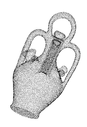
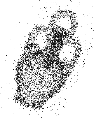
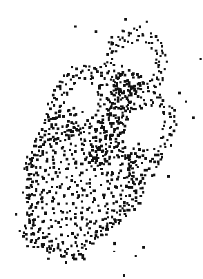
An example of the output of algorithm Declutter is given in Figure 4 (a) – (d). More examples (including for adaptive inputs) can be found in Appendix E .

Extensions.

It turns out that there are many choices that can be used for the $k$-distance $d_{P,k}(x)$ instead of the one introduced in Definition 2.1. Indeed, the goal of $k$-distance intuitively is to provide a more robust distance estimate – Specifically, assume $P$ is a noisy sample of a hidden domain $K\subset\mathbb{X}$. With the presence of noisy points far away from $K$, the distance $d_{\mathbb{X}}(x,P)$ no longer serves as a good approximation of $d_{\mathbb{X}}(x,K)$, the distance from $x$ to the hidden domain $K$. We thus need a more robust distance estimate. The $k$-distance $d_{P,k}(x)$ introduced in Definition 2.1 is one such choice, and there are many other valid choices. As we show in Appendix D, we only need the choice of $d_{P,k}(x)$ to be $1$-Lipschitz, and is less sensitive than $d_{\mathbb{X}}(x,P)$ (that is, $d_{\mathbb{X}}(x,P)\leq d_{P,k}(x)$). We can then define the sampling condition (as in Definitions 2.3 and 2.4) using a different choice of $d_{P,k}(x)$, and Theorems 3.3 and 3.7 still hold. For example, we could replace $k$-distance by $d_{P,k}(x)=\frac{1}{k}\sum_{i=1}^{k}d(x,p_{i}(x))$ where $p_{i}(x)$ is the $i$th nearest neighbor of $x$ in $P$; that is, $d_{P,k}(x)$ is the average distance to the $k$ nearest neighbors of $x$ in $P$. Alternatively, we can replace $k$-distance by $d_{P,k}(x)=d(x,p_{k}(x))$, the distance from $x$ to its $k$-th nearest neighbor in $P$ (which was used in [8] to construct the $\varepsilon$-density net). Declutter algorithm works for all these choices with the same denoising guarantees.

One can in fact further relax the conditions on $d_{P,k}(x)$ or even on the input metric space $(\mathbb{X},d_{\mathbb{X}})$ such that the triangle inequality for $d_{\mathbb{X}}$ only approximately holds. The corresponding guarantees of our Declutter algorithm are provided in Appendix D .

4 Parameter-free decluttering

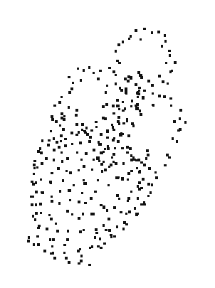
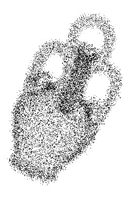
The algorithm Declutter is not entirely satisfactory. First, we need to fix the parameter $k$ a priori. Second, while providing a Hausdorff distance guarantee, this procedure also “sparsifies” input points. Specifically, the empty-ball test also induces some degree of sparsification, as for any point $q$ kept in $Q$, the ball $B(q,2d_{P,k}(q))$ does not contain any other output points in $Q$. While this sparsification property is desirable for some applications, it removes too many points in some cases – See Figure 4 for an example, where the output density is dominated by $\epsilon_{k}$ and does not preserve the dense sampling provided by the input around the hidden compact set $K$. In particular, for $k=9$, it does not completely remove ambient noise, while, for $k=30$, the output is too sparse.

(a)	(b)	(c)	(d)	(e)

Figure 4: (a) – (d) show results of the Algorithm Declutter: (a) the ground truth, (b) the noisy input with 15K points with 1000 ambient noisy points, (c) the output of Algorithm Declutter when $k=9$, (d) the output of Algorithm Declutter when $k=30$. In (e), we show the output of Algorithm ParfreeDeclutter. As shown in Appendix E, algorithm ParfreeDeclutter can remove ambient noise for much sparser input samples with more noisy points.

Data: Point set $P$

Result: Denoised point set $P_{0}$

1 begin

2       Set $i_{*}=\lfloor\log_{2}(|P|)\rfloor$, and $P_{i_{*}}\longleftarrow P$

3      

4      for $i\longleftarrow i_{*}$ to $1$ do

5             $Q\longleftarrow$ Declutter($P_{i}$,$2^{i}$)

6            

7            $P_{i-1}\longleftarrow\cup_{q\in Q}B(q,(10+2\sqrt{2})d_{P_{i},2^{i}}(q))\cap P_{i}$

8            

9      

10

Algorithm 2 ParfreeDeclutter($P$)

In this section, we address both of the above concerns by a novel iterative re-sampling procedure as described in Algorithm ParfreeDeclutter($P$). Roughly speaking, we start with $k=|P|$ and gradually decrease it by halving each time. At iteration $i$, let $P_{i}$ denote the set of points so far kept by the algorithm; $i$ is initialized to be $\lfloor\log_{2}(|P|)\rfloor$ and is gradually decreased. We perform the denoising algorithm Declutter($P_{i},k=2^{i}$) given in the previous section to first denoise $P_{i}$ and obtain a denoised output set $Q$. This set can be too sparse. We enrich it by re-introducing some points from $P_{i}$, obtaining a denser sampling $P_{i-1}\subseteq P_{i}$ of the ground truth. We call this a re-sampling process. This re-sampling step may bring some outliers back into the current set. However, it turns out that a repeated cycle of decluttering and resampling with decreasing values of $k$ removes these outliers progressively. See Figure 2 and also more examples in Appendix E.The entire process remains free of any user supplied parameter. In the end, we show that for an input that satisfies a uniform sampling condition, we can obtain an output set which is both dense and Hausdorff close to the hidden compact set, without the need to know the parameters of the input sampling conditions.

In order to formulate the exact statement of Theorem 4.1, we need to introduce a more relaxed sampling condition. We relax the notion of uniform $(\epsilon_{k},c)$-noisy sample by removing condition $2$. We call it a weak uniform $(\epsilon_{k},c)$-noisy sample. Recall that condition $2$ was the one forbidding the noise to be too dense. So essentially, a weak uniform $(\epsilon_{k},c)$-noisy sample only concerns points on and around the ground truth, with no conditions on outliers.

Theorem 4.1.

Given a point set $P$ and $i_{0}$ such that for all $i>i_{0}$, $P$ is a weak uniform $(\epsilon_{2^{i}},2)$-noisy sample of $K$ and is also a uniform $(\epsilon_{2^{i_{0}}},2)$-noisy sample of $K$, Algorithm ParfreeDeclutter returns a point set $P_{0}\subseteq P$ such that $d_{H}(P_{0},K)\leq(87+16\sqrt{2})\epsilon_{2^{i_{0}}}$.

We elaborate a little on the sampling conditions. On one hand, as illustrated by Figure 1, the uniformity on input points is somewhat necessary in order to obtain a parameter-free algorithm. So requiring a uniform $(\epsilon_{2^{i_{0}}},2)$-noisy sample of $K$ is reasonable. Now it would have been ideal if the theorem only required that $P$ is a uniform $(\epsilon_{2^{i_{0}}},2)$-noisy sample of $K$ for some $k_{0}=2^{i_{0}}$. However, to make sure that this uniformity is not destroyed during our iterative declutter-resample process before we reach $i=i_{0}$, we also need to assume that, around the compact set, the sampling is uniform for any $k=2^{i}$ with $i>i_{0}$ (i.e, before we reach $i=i_{0}$). The specific statement for this guarantee is given in Lemma 4.3. However, while the uniformity for points around the compact set is required for any $i>i_{0}$, the condition that noisy points cannot be arbitrarily dense is only required for one parameter, $k=2^{i_{0}}$.

The constant for the ball radius in the resampling step is taken as $10+2\sqrt{2}$ which we call the resampling constant $C$. Our theoretical guarantees hold with this resampling constant though a value of $4$ works well in practice. The algorithm reduces more noise with decreasing $C$. On the flip side, the risk of removing points causing loss of true signal also increases with decreasing $C$. Section 5 and Appendix E provide several results for Algorithm ParfreeDeclutter. We also point out that while our theoretical guarantee is for non-adaptive case, in practice, the algorithm works well on adaptive sampling as well.

Proof for Theorem 4.1.

Aside from the technical Lemma 4.2 on the $k$-distance, the proof is divided into three steps. First, Lemma 4.3 shows that applying the loop of the algorithm once with parameter $2k$ does not alter the existing sampling conditions for $k^{\prime}\leq k$. This implies that the $\epsilon_{2^{i_{0}}}$-noisy sample condition on $P$ will also hold for $P_{i_{0}}$. Then Lemma 4.4 guarantees that the step going from $P_{i_{0}}$ to $P_{i_{0}-1}$ will remove all outliers. Combined with Theorem 3.3, which guarantees that $P_{i_{0}-1}$ samples well $K$, it guarantees that the Hausdorff distance between $P_{i_{0}-1}$ and $K$ is bounded. However, we do not know $i_{0}$ and we have no means to stop the algorithm at this point. Fortunately, we can prove Lemma 4.5 which guarantees that the remaining iterations will not remove too many points and break the theoretical guarantees – that is, no harm is done in the subsequent iterations even after $i<i_{0}$. Putting all three together leads to our main result Theorem 4.1.

Lemma 4.2.

Given a point set $P$, $x\in\mathbb{X}$ and $0\leq i\leq k$, the distance to the $i$-th nearest neighbor of $x$ in $P$ satisfies, $d_{\mathbb{X}}(x,p_{i})\leq\sqrt{\frac{k}{k-i+1}}d_{P,k}(x)$.

Proof.

The claim is proved by the following derivation.

$$\frac{k-i+1}{k}d_{\mathbb{X}}(x,p_{i})^{2}\leq\frac{1}{k}\sum_{j=i}^{k}d_{\mathbb{X}}(x,p_{j})^{2}\leq\frac{1}{k}\sum_{j=1}^{k}d_{\mathbb{X}}(x,p_{j})^{2}=d_{P,k}(x)^{2}.$$

∎

Lemma 4.3.

Let $P$ be a weak uniform $(\epsilon_{2k},2)$-noisy sample of $K$. For any $k^{\prime}\leq k$ such that $P$ is a (weak) uniform $(\epsilon_{k^{\prime}},c)$-noisy sample of $K$ for some $c$, applying one step of the algorithm, with parameter $2k$ and resampling constant $C=10+2\sqrt{2}$ gives a point set $P^{\prime}\subseteq P$ which is a (weak) uniform $(\epsilon_{k^{\prime}},c)$-noisy sample of $K$.

Proof.

We show that if $P$ is a uniform $(\epsilon_{k^{\prime}},c)$-noisy sample of $K$, then $P^{\prime}$ will also be a uniform $(\epsilon_{k^{\prime}},c)$-noisy sample of $K$. The similar version for weak uniformity follows from the same argument.

First, it is easy to see that as $P^{\prime}\subset P$, the second and third sampling conditions of Def. 2.4 hold for $P^{\prime}$ as well. What remains is to show that Condition 1 also holds.

Take an arbitrary point $x\in K$. We know that $d_{P,2k}(x)\leq\epsilon_{2k}$ as $P$ is a weak uniform $(\epsilon_{2k},2)$-noisy sample of $K$. Hence there exists $p\in P$ such that $d_{\mathbb{X}}(p,x)\leq d_{P,2k}(x)\leq\epsilon_{2k}$ and $d_{P,2k}(p)\leq 2\epsilon_{2k}$. Writing $Q$ the result of the decluttering step, $\exists q\in Q$ such that $d_{\mathbb{X}}(p,q)\leq 2d_{P,2k}(p)\leq 4\epsilon_{2k}$. Moreover, $d_{P,2k}(q)\geq\frac{\epsilon_{2k}}{2}$ due to the uniformity condition for $P$.

Using Lemma 4.2, for $k^{\prime}\leq k$, the $k^{\prime}$ nearest neighbors of $x$, which are chosen from $P$, $NN_{k^{\prime}}(x)$ satisfies:

$$NN_{k^{\prime}}(x)\subset B(x,\sqrt{2}\epsilon_{2k})\subset B(p,(1+\sqrt{2})\epsilon_{2k})\subset B(q,(5+\sqrt{2})\epsilon_{2k})\subset B(q,(10+2\sqrt{2})d_{P,2k}(q))$$

Hence $NN_{k^{\prime}}(x)\subset P^{\prime}$ and $d_{P^{\prime},k^{\prime}}(x)=d_{P,k^{\prime}}(x)\leq\epsilon_{k}$. This proves the lemma. ∎

Lemma 4.4.

Let $P$ be a uniform $(\epsilon_{k},2)$-noisy sample of $K$. One iteration of decluttering and resampling with parameter $k$ and resampling constant $C=10+2\sqrt{2}$ provides a set $P^{\prime}\subseteq P$ such that $\delta_{H}(P^{\prime},K)\leq 8C\epsilon_{k}+7\epsilon_{k}$.

Proof.

Let $Q$ denote the output after the decluttering step. Using Theorem 3.3 we know that $\delta_{H}(Q,K)\leq 7\epsilon_{k}$. Note that $Q\subset P^{\prime}$. Thus, we only need to show that for any $p\in P^{\prime}$, $d_{\mathbb{X}}(p,K)\leq 8C\epsilon_{k}+7\epsilon_{k}$. Indeed, by the way the algorithm removes points, for any $p\in P^{\prime}$, there exists $q\in Q$ such that $p\in B(q,Cd_{P,k}(q))$. It then follows that

$$d_{\mathbb{X}}(p,K)\leq Cd_{P,k}(q)+d_{\mathbb{X}}(q,K)\leq C(\epsilon_{k}+d_{\mathbb{X}}(q,K))+7\epsilon_{k}\leq 8C\epsilon_{k}+7\epsilon_{k}.$$

∎

Lemma 4.5.

Given a point $y\in P_{i}$, there exists $p\in P_{0}$ such that $d_{\mathbb{X}}(y,p)\leq\kappa d_{P_{i},2^{i}}(y)$, where $\kappa=\frac{18+17\sqrt{2}}{4}$.

Proof.

We show this lemma by induction on $i$. First for $i=0$ the claim holds trivially. Assuming that the result holds for all $j<i$ and taking $y\in P_{i}$, we distinguish three cases.

Case 1: $y\in P_{i-1}$ and $d_{P_{i-1},2^{i-1}}(y)\leq d_{P_{i},2^{i}}(y)$.
Applying the recurrence hypothesis for $j=i-1$ gives the result immediately.

Case 2: $y\notin P_{i-1}$.    It means that $y$ has been removed by decluttering and not been put back by resampling. These together imply that there exists $q\in Q_{i}\subseteq P_{i-1}$ such that $d_{\mathbb{X}}(y,q)\leq 2d_{P_{i},2^{i}}(y)$ and $d_{\mathbb{X}}(y,q)>Cd_{P_{i},2^{i}}(q)$ with $C=10+2\sqrt{2}$. From the proof of Lemma 4.3, we know that the $2^{i-1}$ nearest neighbors of $q$ in $P_{i}$ are resampled and included in $P_{i-1}$. Therefore, $d_{P_{i-1},2^{i-1}}(q)=d_{P_{i},2^{i-1}}(q)\leq d_{P_{i},2^{i}}(q)$. Moreover, since $q\in P_{i-1}$, the inductive hypothesis implies that there exists $p\in P_{0}$ such that $d_{\mathbb{X}}(p,q)\leq\kappa d_{P_{i-1},2^{i-1}}(q)\leq\kappa d_{P_{i},2^{i}}(q)$. Putting everything together, we get that there exists $p\in P_{0}$ such that

$$d_{\mathbb{X}}(p,y)\leq d_{\mathbb{X}}(p,q)+d_{\mathbb{X}}(q,y)\leq\kappa d_{P_{i},2^{i}}(q)+2d_{P_{i},2^{i}}(y)\leq\left(\frac{\kappa}{5+\sqrt{2}}+2\right)d_{P_{i},2^{i}}(y)\leq\kappa d_{P_{i},2^{i}}(y).$$

The derivation above also uses the relation that $d_{P_{i},2^{i}}(q)<\frac{1}{C}d_{\mathbb{X}}(y,q)\leq\frac{2}{C}d_{P_{i},2^{i}}(y)$.

Case 3: $y\in P_{i-1}$ and $d_{P_{i-1},2^{i-1}}(y)>d_{P_{i},2^{i}}(y)$.
The second part implies that at least one of the $2^{i-1}$ nearest neighbors of $y$ in $P_{i}$ does not belong to $P_{i-1}$. Let $z$ be such a point. Note that $d_{\mathbb{X}}(y,z)\leq\sqrt{2}d_{P_{i},2^{i}}(y)$ by Lemma 4.2. For point $z$, we can apply the second case and therefore, there exists $p\in P_{0}$ such that

$$d_{\mathbb{X}}(p,y) \leq d_{\mathbb{X}}(p,z)+d_{\mathbb{X}}(z,y)\leq\left(\frac{\kappa}{5+\sqrt{2}}+2\right)d_{P_{i},2^{i}}(z)+\sqrt{2}d_{P_{i},2^{i}}(y)$$

$$\leq\left(\frac{\kappa}{5+\sqrt{2}}+2\right)\left(d_{P_{i},2^{i}}(y)+d_{\mathbb{X}}(z,y)\right)+\sqrt{2}d_{P_{i},2^{i}}(y)$$

$$\leq\left(\left(\frac{\kappa}{5+\sqrt{2}}+2\right)(1+\sqrt{2})+\sqrt{2}\right)d_{P_{i},2^{i}}(y)\leq\kappa d_{P_{i},2^{i}}(y)$$

∎

Putting everything together.  A repeated application of Lemma 4.3 (with weak uniformity) guarantees that $P_{i_{0}+1}$ is a weak uniform $(\epsilon_{2^{i_{0}+1}},2)$-noisy sample of $K$. One more application (with uniformity) provides that $P_{i_{0}}$ is a uniform $(\epsilon_{2^{i_{0}}},2)$-noisy sample of $K$. Thus, Lemma 4.4 implies that $d_{H}(P_{i_{0}-1},K)\leq(87+16\sqrt{2})\epsilon_{2^{i_{0}}}$. Notice that $P_{0}\subset P_{i_{0}-1}$ and thus for any $p\in P_{0}$, $d_{\mathbb{X}}(p,K)\leq(87+16\sqrt{2})\epsilon_{2^{i_{0}}}$.

To show the other direction, consider any point $x\in K$. Since $P_{i_{0}}$ is a uniform $(\epsilon_{2^{i_{0}}},2)$-noisy sample of $K$, there exists $y\in P_{i_{0}}$ such that $d_{\mathbb{X}}(x,y)\leq\epsilon_{2^{i_{0}}}$ and $d_{P_{i_{0}},2^{i_{0}}}(y)\leq 2\epsilon_{2^{i_{0}}}$. Applying Lemma 4.5, there exists $p\in P_{0}$ such that $d_{\mathbb{X}}(y,p)\leq\frac{18+17\sqrt{2}}{2}\epsilon_{2^{i_{0}}}$. Hence $d_{\mathbb{X}}(x,p)\leq\left(\frac{18+17\sqrt{2}}{2}+1\right)\epsilon_{2^{i_{0}}}\leq(87+16\sqrt{2})\epsilon_{2^{i_{0}}}$. The theorem then follows. $\blacksquare$

5 Preliminary experimental results

We now present some preliminary experimental results for the two denoising algorithms developed in this paper. See Appendix E for more results.

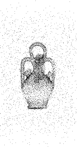
In Figure 5, we show different stages of the ParfreeDeclutter algorithm on an input with adaptively sampled points. Even though for the parameter-free algorithm, theoretical guarantees are only provided for uniform samples, we note that it performs well on this adaptive case as well.

Figure 5: Experiment on a two dimensional manifold in three dimensions. From left to right, the ground truth, the noisy adaptively sampled input, output of two intermediate steps of Algorithm ParfreeDeclutter, and the final result.

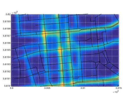
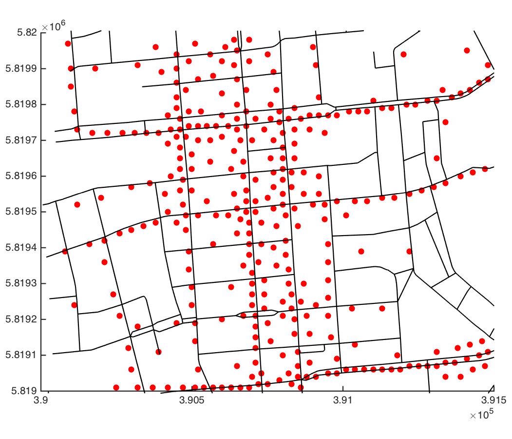
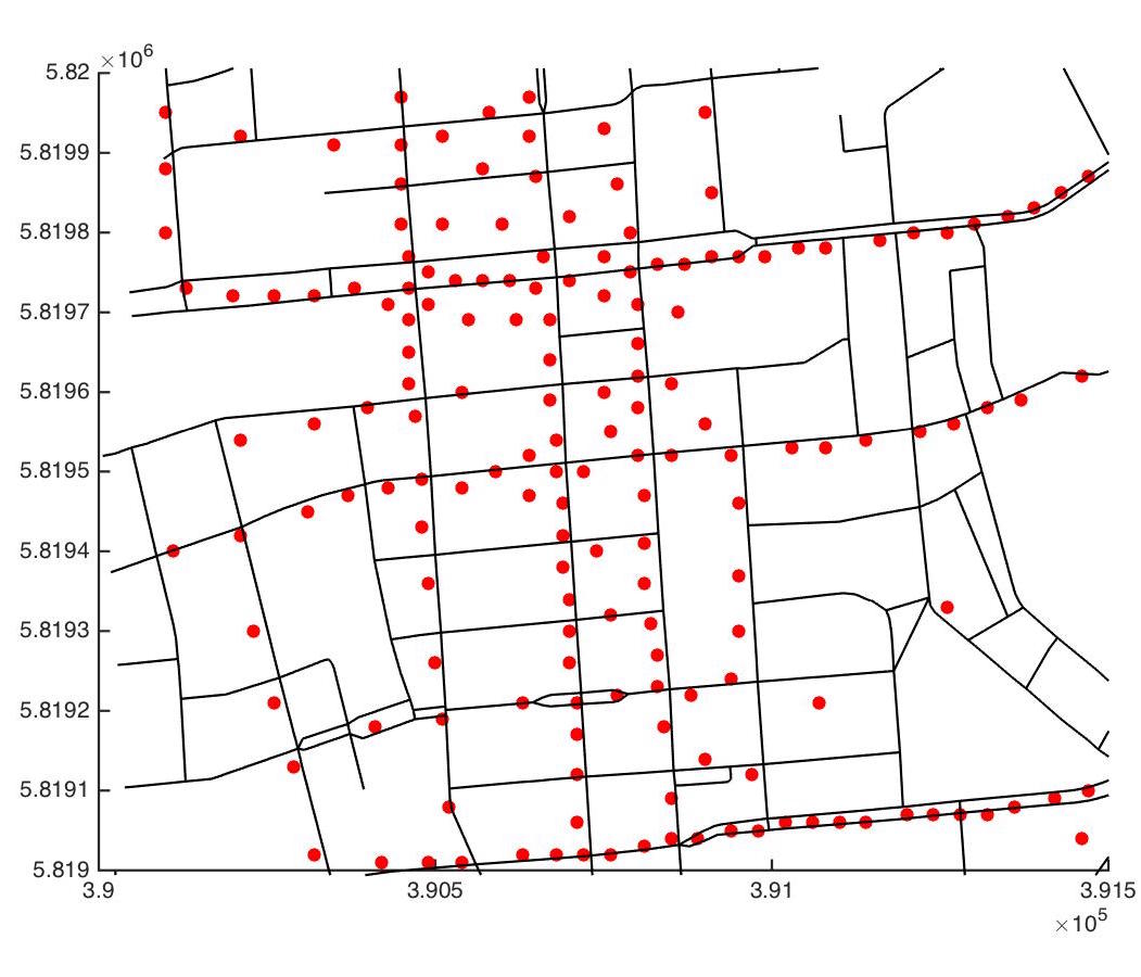
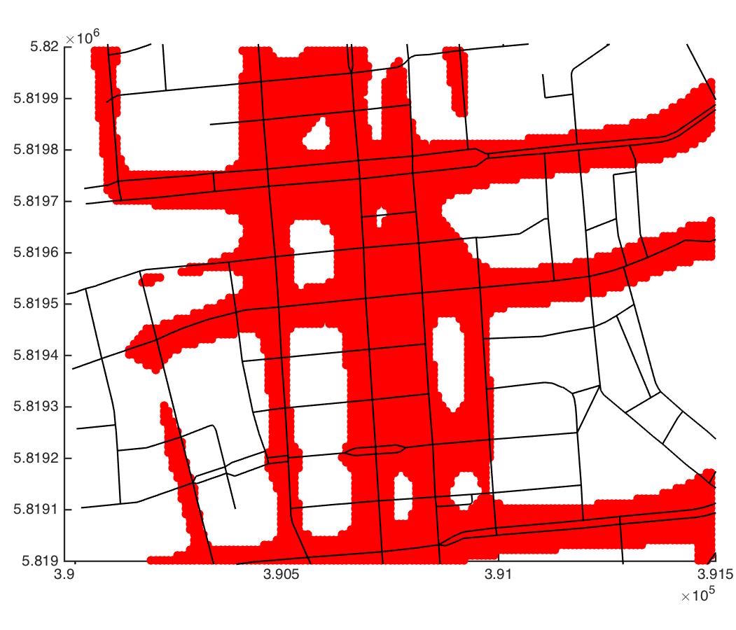
A second example is given in Figure 6. Here, the input data is obtained from a set of noisy GPS trajectories in the city of Berlin. In particular, given a set of trajectories (each modeled as polygonal curves), we first convert it to a density field by KDE (kernel density estimation). We then take the input as the set of grid points in 2D where every point is associated with a mass (density). Figure 6 (a) shows the heat-map of the density field where light color indicates high density and blue indicates low density. In (b) and (c), we show the output of our Declutter algorithm (the ParfreeDeclutter algorithm does not provide good results as the input is highly non-uniform) for $k$ = 40 and $k=75$ respectively. In (d), we show the set of 40$\%$ points with the highest density values. The sampling of the road network is highly non-uniform. In particular, in the middle portion, even points off the roads have very high density due to noisy input trajectories. Hence a simple thresholding cannot remove these points and the output in (d) fills the space between roads in the middle portion; however more aggressive thresholding will cause loss of important roads. Our Declutter algorithm can capture the main road structures without collapsing nearby roads in the middle portion though it also sparsifies the data.

(a)	(b)	(c)	(d)

Figure 6: (a) The heat-map of a density field generated from GPS traces. There are around 15k (weighted) grid points serving as an input point set. The output of Algorithm Declutter when (b) $k=40$ and (c) $k=75$, (d) thresholding of 40% points with the highest density.

In another experiment, we apply the denoising algorithm as a pre-processing for high-dimensional data classification. Here we use MNIST data sets, which is a database of handwritten digits from ’0’ to ’9’. Table 1 shows the experiment on digit 1 and digit 7. We take a random collection of 1352 images of digit ’1’ and 1279 images of digit ’7’ correctly labeled as a training set, and take 10816 images of digit 1 and digit 7 as a testing set. Each of the image is $28\times 28$ pixels and thus can be viewed as a vector in $\mathbb{R}^{784}$. We use the $L_{1}$ metric to measure distance between such image-vectors. We use a linear SVM to classify the 10816 testing images. The classification error rate for the testing set is $0.6564\%$ shown in the second row of Table 1.

Next, we artificially add two types of noises to input data: the swapping-noise and the background-noise. The swapping-noise means that we randomly mislabel some images of ‘1’ as ’7’, and some images of ‘7’ as ’1’. As shown in the third row of Table 1, the classification error increases to about $4.096\%$ after such mislabeling in the training set.

Next, we apply our ParfreeDeclutter algorithm to this training set with added swapping-noise (to the set of images with label ’1’ and the set with label ’7’ separately) to first clean up the training set. As we can see in Row-6 of Table 1, we removed most images with a mislabeled ‘1’ (which means the image is ’7’ but it is labeled as ’1’). A discussion on why mislabeled ‘7’s are not removed is given in Appendix E. We then use the denoised dataset as the new training set, and improved the classification error to $2.45\%$.

The second type of noise is the background noise, where we replace the black backgrounds of a random subset of images in the training set (250 ‘1’s and 250 ‘7’s) with some other grey-scaled images. Under such noise, the classification error increases to $1.146\%$. Again, we perform our ParfreeDeclutter algorithm to denoise the training sets, and use the denoised data sets as the new training set. The classification error is then improved to $0.7488\%$. More results on the MNIST data sets are reported in Appendix E.

1						Error(%)
2	Original	# Digit 1 1352		# Digit 7 1279		0.6564
3	Swap. Noise	# Mislabelled 1 270		# Mislabelled 7 266		4.0957
4		Digit 1		Digit 7
5		# Removed	# True Noise	# Removed	# True Noise
6	L1 Denoising	314	264	17	1	2.4500

7	Back. Noise	# Noisy 1 250		# Noisy 7 250		1.1464
8		Digit 1		Digit 7
9		# Removed	# True Noise	# Removed	# True Noise
10	L1 Denoising	294	250	277	250	0.7488

Table 1: Results of denoising on digit 1 and digit 7 from the MNIST.

6 Discussions

Parameter selection is a notorious problem for many algorithms in practice. Our high level goal is to understand the roles of parameters in algorithms for denoising, how to reduce their use and what theoretical guarantees do they entail. While this paper presented some results towards this direction, many interesting questions ensue. For example, how can we further relax our sampling conditions, making them allow more general inputs, and how to connect them with other classical noise models?

We also note that while the output of ParfreeDeclutter is guaranteed to be close to the ground truth w.r.t. the Hausdorff distance, this Hausdorff distance itself is not estimated. Estimating this distance appears to be difficult. We could estimate it if we knew the correct scale, i.e. $i_{0}$, to remove the ambiguity. Interestingly, even with the uniformity condition, it is not clear how to estimate this distance in a parameter free manner.

We do not provide guarantees for the parameter-free algorithm in an adaptive setting though the algorithm behaved well empirically for the adaptive case too. A partial result is presented in Appendix B , but the need for a small $\epsilon_{k}$ in the conditions defeat the attempts to obtain a complete result.

The problem of parameter-free denoising under more general sampling conditions remains open. It may be possible to obtain results by replacing uniformity with other assumptions, for example topological assumptions: say, if the ground truth is a simply connected manifold without boundaries, can this help to denoise and eventually reconstruct the manifold?

Acknowledgments

We thank Ken Clarkson for pointing out the result in [8]. This work is in part supported by National Science Foundation via grants CCF-1618247, CCF-1526513, CCF-1318595 and IIS-1550757.

Appendix A Missing details from section 3

Proof of Lemma 3.5.

Let $x$ be a point of $K$. Then there exists $i$ such that $d_{\mathbb{X}}(p_{i},x)\leq d_{P,k}(x)\leq\epsilon_{k}f(x)$. If $p_{i}$ belongs to $Q$, then setting $q=p_{i}$ proves the lemma. Otherwise, because of the way that the algorithm eliminates points, there must exist $j<i$ such that $p_{j}\in Q_{i-1}\subseteq Q$ and

$$d_{\mathbb{X}}(p_{i},p_{j})\leq 2d_{P,k}(p_{i})\leq 2(d_{P,k}(x)+d_{\mathbb{X}}(p_{i},x))\leq 4\epsilon_{k}f(x),$$

the second inequality follows from the 1-Lipschitz property of $d_{P,k}$ function and the sampling Condition 1. Then

$$d_{\mathbb{X}}(x,p_{j})\leq d_{\mathbb{X}}(x,p_{i})+d_{\mathbb{X}}(p_{i},p_{j})\leq 5\epsilon_{k}f(x).$$

Proof of Lemma 3.6.

Consider any $p_{i}\in P$ and let $\bar{p}_{i}$ be one of its nearest points in $K$. It is sufficient to show that if $d_{\mathbb{X}}(p_{i},\bar{p}_{i})>7\epsilon_{k}f(\bar{p}_{i})$, then $p_{i}\notin Q$ .

By Condition 2 of Def. 2.6, $d_{P,k}(p_{i})\geq d_{\mathbb{X}}(p_{i},\bar{p}_{i})-\epsilon_{k}f(\bar{p}_{i})>6\epsilon_{k}f(\bar{p}_{i})$. By Lemma 3.5, there exists $q\in Q$ such that $d_{\mathbb{X}}(\bar{p}_{i},q)\leq 5\epsilon_{k}f(\bar{p}_{i})$. Thus,

$$d_{P,k}(q)\leq d_{P,k}(\bar{p}_{i})+d_{\mathbb{X}}(\bar{p}_{i},q)\leq 6\epsilon_{k}f(\bar{p}_{i}).$$

Therefore, $d_{P,k}(p_{i})>6\epsilon_{k}f(\bar{p}_{i})\geq d_{P,k}(q)$ implying that $q\in Q_{i-1}$. Combining triangle inequality and Condition 2 of Def. 2.6, we have

$$d_{\mathbb{X}}(p_{i},q)\leq d_{\mathbb{X}}(p_{i},\bar{p}_{i})+d_{\mathbb{X}}(\bar{p}_{i},q)\leq d_{P,k}(p_{i})+\epsilon_{k}f(\bar{p}_{i})+5\epsilon_{k}f(\bar{p}_{i})<2d_{P,k}(p_{i}).$$

Therefore, $q\in Q_{i-1}\cap B(p_{i},2d_{P,k}(p_{i}))$, meaning that $p_{i}\notin Q$.

Hence, we have a point of $Q_{i-1}$ inside the ball of center $p_{i}$ and radius $2d_{P,k}(p_{i})$, which guarantees that $p_{i}$ is not selected. The lemma then follows.

Appendix B Towards parameter-free denoising for adaptive case

Unfortunately, our parameter-free denoising algorithm does not fully work in the adaptive setting. We can still prove that one iteration of the loop works. However, the value chosen for the resampling constant $C$ has to be sufficiently large with respect to $\epsilon_{k}$. This condition is not satisfied when $k$ is large as $\epsilon_{k}$ in that case is very large.

Theorem B.1.

Let $P$ be a point set that is both a uniform $(\epsilon_{2k},2)$-adaptive noisy sample and a uniform $(\epsilon_{k},2)$-adaptive noisy sample of $K$. Applying one step of the ParfreeDeclutter algorithm with parameter $2k$ gives a point set $P^{\prime}$ which is a uniform $(\epsilon_{2k},2)$-adaptive noisy sample of $K$ when $\epsilon_{2k}$ is sufficiently small and the resampling constant $C$ is sufficiently large.

Proof.

As in the global conditions case, only the first condition has to be checked. Let $x\in K$ then, following the proof of Lemma 3.5, there exists $q\in P^{\prime}$ such that $d_{\mathbb{X}}(x,q)\leq 5\epsilon_{2k}$ and $d_{P,2k}(q)\leq 2\epsilon_{2k}$. The feature size $f$ is 1-Lipschitz and thus:

$$f(x) \leq f(\bar{q})+d_{\mathbb{X}}(\bar{q},x)$$

$$\leq f(\bar{q})+d_{\mathbb{X}}(q,\bar{q})+d_{\mathbb{X}}(q,x)$$

$$\leq f(\bar{q})+d_{P,2k}(q)+\epsilon_{2k}f(\bar{q})+5\epsilon_{2k}f(x)$$

Hence

$$f(\bar{q})\geq\frac{1-7\epsilon_{2k}}{1+\epsilon_{2k}}f(x).$$

Therefore $d_{P,2k}(q)\geq\frac{1-7\epsilon_{2k}}{1+\epsilon_{2k}}\frac{\epsilon_{2k}}{2}f(x)$. The claimed result is obtained if the constant $C$ satisfies $C\geq\frac{2(5+\sqrt{2})(1+\epsilon_{2k})}{1-7\epsilon_{2k}}$ as $B(x,\sqrt{2}\epsilon_{2k}f(x))\subset B(q,Cd_{P,2k}(q))$. ∎

Appendix C Application to topological data analysis

In this section, we provide an example of using our decluttering algorithm for topology inference. We quickly introduce notations for some notions of algebraic topology and refer the reader to [17, 20, 24] for the definitions and basic properties. Our approaches mostly use standard arguments from the literature of topology inference; e.g, [5, 11, 14].

Given a topological space $X$, we denote $H_{i}(X)$ its $i$-dimensional homology group with coefficients in a field. As all our results are independent of $i$, we will write $H_{*}(X)$. We consider the persistent homology of filtrations obtained as sub-level sets of distance functions. Given a compact set $K$, we denote the distance function to $K$ by $d_{K}$. We moreover assume that the ambient space is triangulable which ensures that these functions are tame and the persistence diagram $\mathrm{Dgm}(d_{K}^{-1})$ is well defined. We use $d_{B}$ for the bottleneck distance between two persistence diagrams. We recall the main theorem from [12] which implies:

Proposition C.1.

Let $A$ and $B$ be two triangulable compact sets in a metric space. Then,

$$d_{B}(\mathrm{Dgm}(d_{A}^{-1}),\mathrm{Dgm}(d_{B}^{-1}))\leq d_{H}(A,B).$$

This result trivially guarantees that the result of our decluttering algorithm allows us to approximate the persistence diagram of the ground truth.

Corollary C.2.

Given a point set $P$ which is an $\epsilon_{k}$-noisy sample of a compact set $K$, the Declutter algorithm returns a set $Q$ such that

$$d_{B}(\mathrm{Dgm}(d_{K}^{-1}),\mathrm{Dgm}(d_{Q}^{-1}))\leq 7\epsilon_{k}.$$

The algorithm reduces the size of the set needed to compute an approximation diagram. Previous approaches relying on the distance to a measure to handle noise ended up with a weighted set of size roughly $n^{k}$ or used multiplicative approximations which in turn implied a stability result at logarithmic scale for the Bottleneck distance [6, 19]. The present result uses an unweighted distance to compute the persistence diagram and provides guarantees without the logarithmic scale using fewer points than before.

If one is interested in inferring homology instead of computing a persistence diagram, our previous results guarantee that the Čech complex $C_{\alpha}(Q)$ or the Rips complex $R_{\alpha}(Q)$ can be used. Following [11], we use a nested pair of filtration to remove noise. Given $A\subset B$, we consider the map $\phi$ induced at the homology level by the inclusion $A\hookrightarrow B$. We denote $H_{*}(A\hookrightarrow B)=\mathrm{Im}(\phi)$. More precisely, denoting $K^{\lambda}=d_{K}^{-1}(\lambda)$ and $\mathrm{wfs}$ as the weak feature size, we obtain:

Proposition C.3.

Let $P$ be an $\epsilon_{k}$-noisy sample of a compact set $K\subset\mathbb{R}^{d}$ with $\epsilon_{k}<\frac{1}{28}\mathrm{wfs}(K)$. Let $Q$ be the output of Declutter($P$). Then for all $\alpha$, $\alpha^{\prime}\in[7\epsilon_{k},\mathrm{wfs}(K)-7\epsilon_{k}]$ such that $\alpha^{\prime}-\alpha>14\epsilon_{k}$ and for all $\lambda\in(0,\mathrm{wfs}(K))$, we have

$$H_{*}(K^{\lambda})\cong H_{*}(C_{\alpha}(Q)\hookrightarrow C_{\alpha^{\prime}}(Q))$$

Proposition C.4.

Let $P$ be an $\epsilon_{k}$-noisy sample of a compact set $K\subset\mathbb{R}^{d}$ with $\epsilon_{k}<\frac{1}{35}\mathrm{wfs}(K)$. Let $Q$ be the output of Declutter($P$). Then for all $\alpha\in[7\epsilon_{k},\frac{1}{4}(\mathrm{wfs}(K)-7\epsilon_{k})]$ and $\lambda\in(0,\mathrm{wfs}(K))$, we have

$$H_{*}(K^{\lambda})\cong H_{*}(R_{\alpha}(Q)\hookrightarrow R_{4\alpha}(Q))$$

These two propositions are direct consequences of [11, Theorems 3.5 & 3.6]. To be used, both these results need the input of one or more parameters, $\alpha$ and $\alpha^{\prime}$, corresponding to a choice of scale. This cannot be avoided as it is equivalent to estimating the Hausdorff distance between a point set and an unknown compact set, problem discussed in the introduction. However, by adding a uniformity hypothesis and knowing the uniformity constant $c$, the problem can be solved. We use the fact that the minimum $d_{P,k}$ over the point set $P$ is bounded from below. Let us write $\kappa=\min_{p\in P}d_{P,k}(p)$.

Lemma C.5.

If $P$ is an $\epsilon_{k}$-noisy sample of $K$ then $\kappa\leq 2\epsilon_{k}$.

Proof.

Let $x\in K$, then there exists $p\in P$ such that $d_{\mathbb{X}}(x,p)\leq d_{P,k}(x)\leq\epsilon_{k}$. Therefore $\kappa\leq d_{P,k}(p)\leq d_{P,k}(x)+d_{\mathbb{X}}(x,p)\leq 2\epsilon_{k}$. ∎

This trivial observation has the consequence that $c$ is greater than $\frac{1}{2}$ in any uniform $(\epsilon_{k},c)$-noisy sample. We can compute $c\kappa$ and use it to define an $\alpha$ for using the previous propositions. We formulate the conditions precisely in the following propositions. Note that the upper bound for $\alpha$ is not necessarily known. However, the conditions imply that the interval of correct values for $\alpha$ is non-empty.

Proposition C.6.

Let $P$ be a uniform $(\epsilon_{k},c)$-noisy sample of a compact set $K\subset\mathbb{R}^{d}$ with $c\epsilon_{k}<\frac{1}{56}\mathrm{wfs}(K)$. Let $Q$ be the output of Declutter($P$). Then for all $\alpha$, $\alpha^{\prime}\in[7c\kappa,\mathrm{wfs}(K)-7c\epsilon_{k}]$ such that $\alpha^{\prime}-\alpha>14c\kappa$ and for all $\lambda\in(0,\mathrm{wfs}(K))$, we have

$$H_{*}(K^{\lambda})\cong H_{*}(C_{\alpha}(Q)\hookrightarrow C_{\alpha^{\prime}}(Q))$$

Proof.

Following Proposition C.3, we need to choose $\alpha$ and $\alpha^{\prime}$ inside the interval $[7\epsilon_{k},\mathrm{wfs}(K)-7\epsilon_{k}]$. Using the third hypothesis, we know that $7c\kappa\geq 7c\epsilon_{k}$. We need to show that $\alpha$ and $\alpha^{\prime}$ exist, i.e. $21c\kappa<\mathrm{wfs}(K)-7\epsilon_{k}$. Recall that $c\geq 2$ , $\kappa\leq 2\epsilon_{k}$. Therefore, $21c\kappa+7\epsilon_{k}\leq 56c\epsilon_{k}<\mathrm{wfs}(K)$. ∎

Proposition C.7.

Let $P$ be a uniform $(\epsilon_{k},c)$-noisy sample of a compact set $K\subset\mathbb{R}^{d}$ with $c\epsilon_{k}<\frac{1}{70}\mathrm{wfs}(K)$. Let $Q$ be the output of Declutter($P$). Then for all $\alpha\in[7c\kappa,\frac{1}{4}(\mathrm{wfs}(K)-7\epsilon_{k})]$ and $\lambda\in(0,\mathrm{wfs}(K))$, we have

$$H_{*}(K^{\lambda})\cong H_{*}(R_{\alpha}(Q)\hookrightarrow R_{4\alpha}(Q))$$

The proof is similar to the one for the previous proposition. Note that even if the theoretical bound can be larger, we can always pick $\alpha=7c\kappa$ in the second case and the proof works. The sampling conditions on these results can be weakened by using the more general notion of $(\epsilon_{k},r,c)$-sample of [4], assuming that $r$ is sufficiently large with respect to $\epsilon_{k}$.

Appendix D Extensions for Declutter algorithm

It turns out that our Declutter algorithm can be run with different choices for the $k$-distance $d_{P,k}(x)$ as introduced in Definition 2.1 which still yields similar denosing guarantees.

Specifically, assume that we now have a certain robust distance estimate $d_{P,k}(x)$ for each point $x\in\mathbb{X}$ such that the following properties are satisfied.

Conditions for $d_{P,k}$

.
(A) For any $x\in\mathbb{X}$, $d_{\mathbb{X}}(x,P)\leq d_{P,k}(x)$; and
(B) $d_{P,k}$ is $1$-Lipschitz, that is, for any $x,y\in\mathbb{X}$ we have $d_{P,k}(x)\leq d_{P,k}(y)+d(x,y)$.

Examples

.
(1) We can set $d_{P,k}$ to be the average distance to $k$ nearest neighbors in $P$; that is, for any $x\in\mathbb{X}$, define $d_{P,k}(x)=\frac{1}{k}\sum_{i=1}^{k}d(x,p_{i}(x))$ where $p_{i}(x)$ is the $i$th nearest neighbor of $x$ in $P$. We refer to this as the average $k$-distance. It is easy to show that the average $k$-distance satisfies the two conditions above.
(2) We can set $d_{P,k}(x)$ to be the distance from $x$ to its $k$-th nearest neighbors in $P$; that is, $d_{P,k}(x)=d_{\mathbb{X}}(x,p_{k}(x))$. We refer to this distance as $k$-th NN-distance.

We can then define the sampling condition (as in Definitions 2.3 and 2.4) based on our choice of $d_{P,k}$ as before. Notice that, under different choices of $d_{P,k}$, $P$ will be an $\varepsilon_{k}$-noisy sample for different values of $\varepsilon_{k}$. Following the same arguments as in Section 3, we can show that Theorems 3.3 and 3.7 still hold as long as $d_{P,k}$ satisfies the two conditions above. For clarity, we provide an explicit statement for the analog of Theorem 3.3 below and omit the corresponding statement for Theorem 3.7.

Theorem D.1.

Given a $\epsilon_{k}$-noisy sample $P$ of a compact set $K\subseteq\mathbb{X}$ under a choice of $d_{P,k}$ that satisfies the conditions (A) and (B) as stated above, Algorithm Declutter returns a set $Q\subseteq P$ such that

$$d_{H}(K,Q)\leq 7\epsilon_{k}.$$

We remark that in [8], Chan et al. proposed to use the $k$-th NN-distance to generate the so-called $\varepsilon$-density net, where $k=\varepsilon n$. The criterion to remove points from $P$ to generate $Q$ in their procedure is slightly different from our Declutter algorithm. However, it is easy to show that the output of their procedure (which is a $k/n$-density net) satisfies the same guarantee as the output of the Declutter algorithm does (Theorem D.1).

Further extensions.  One can in fact further relax the conditions on $d_{P,k}(x)$ or even on the input metric space $(\mathbb{X},d_{\mathbb{X}})$ such that the triangle inequality for $d_{\mathbb{X}}$ only approximately holds. In particular, we assume that

Relaxation-1

. $d_{\mathbb{X}}(x,y)\leq{c_{\mathbb{X}}}[d_{\mathbb{X}}(x,w)+d_{\mathbb{X}}(w,y)]$, for any $x,y,w\in\mathbb{X}$, with ${c_{\mathbb{X}}}\geq 1$. That is, the input ambient space $(X,d_{\mathbb{X}})$ is almost a metric space where the triangle inequality holds with a multiplicative factor.

Relaxation-2

. $d_{P,k}(x)\leq{c_{Lip}}[d_{P,k}(y)+d_{\mathbb{X}}(x,y)]$, for any $x,y\in\mathbb{X}$ with ${c_{Lip}}\geq 1$. That is, the $1$-Lipschitz condition on $d_{P,k}$ is also relaxed to have a multiplicative factor.

We then obtain the following analog of Theorem 3.3:

Theorem D.2.

Suppose $(\mathbb{X},d_{\mathbb{X}})$ is a space where $d_{\mathbb{X}}$ satisfies Relaxation-1 above. Let $d_{P,k}$ be a robust distance function w.r.t. $P$ that satisfies Condition (A) and Relaxation-2 defined above. Given a point set $P$ which is an $\epsilon_{k}$-noisy sample of a compact set $K\subseteq\mathbb{X}$ under the choice of $d_{P,k}$, Algorithm Declutter returns a set $Q\subseteq P$ such that

$$d_{H}(K,Q)\leq m\epsilon_{k}$$

where $m=max\left\{{c_{Lip}}+{c_{\mathbb{X}}}{c_{Lip}}+4{c_{\mathbb{X}}}{c_{Lip}}^{2}+1,\frac{2+{c_{\mathbb{X}}}^{2}+4{c_{\mathbb{X}}}^{2}{c_{Lip}}}{2-{c_{\mathbb{X}}}}\right\}.$

Finally, we remark that a different way to generalize the 1-Lipschitz condition for $d_{P,k}(x)$ is by asserting $d_{P,k}(x)-d_{P,k}(y)\leq{c_{Lip}}d_{\mathbb{X}}(x,y)$. We can use this to replace Relaxation-2 and obtain a similar guarantee as in the above theorem. We can also further generalize Relaxation-2 by allowing an additive term as well. We omit the resulting bound on the output of the Declutter algorithm.

Appendix E Experimental results

In this section, we provide more details of our empirical results, an abridged version of which already appeared in the main text. We start with the decluterring algorithm. This algorithm needs the input of a parameter $k$. This parameter has a direct influence on the result. On one hand, if $k$ is too small, not all noisy points are removed from the sample. On the other hand, if $k$ is too large, we remove too many points and end up with a very sparse sample that is unable to describe the underlying object precisely.

Experiments for Declutter algorithm.

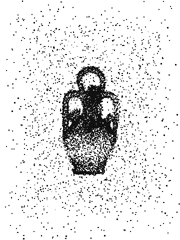
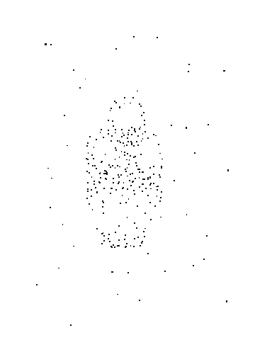
Figure 7 presents results of Algorithm Declutter for the so-called Botijo example. In this case, no satisfying $k$ can be found. A parameter $k$ that is sufficiently large to remove the noise creates an output set that is too sparse to describe the ground truth well.

Figure 7: From left to right, the ground truth, the noisy input and the output of Algorithm Declutter for $k=81$ and $k=148$

We further illustrate the behavior of our algorithm by looking at the Hausdorff distance between the output and the ground truth, and at the cardinality of the output, in the function of $k$ (Figure 8). Note that the Hausdorff distance drops suddenly when we remove the last of the outliers. However, it is already too late to represent the ground truth well as only a handful of points are kept at this stage. While sparsity is often a desired property, here it becomes a hindrance as we are no longer able to describe the underlying set.

Figure 8: Hausdorff distance between the ground truth and the output of the declutter algorithm, and cardinality of this output in the function of $k$.

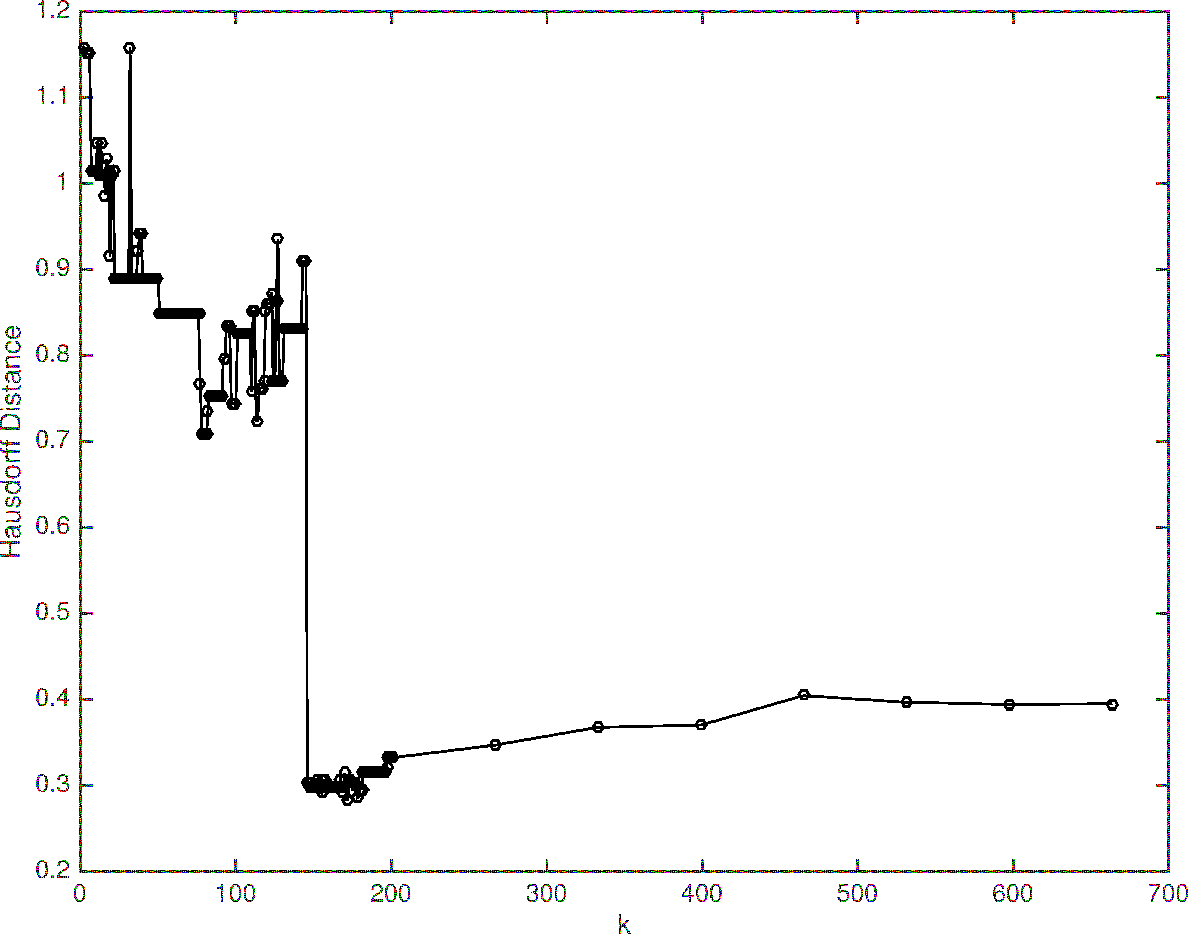
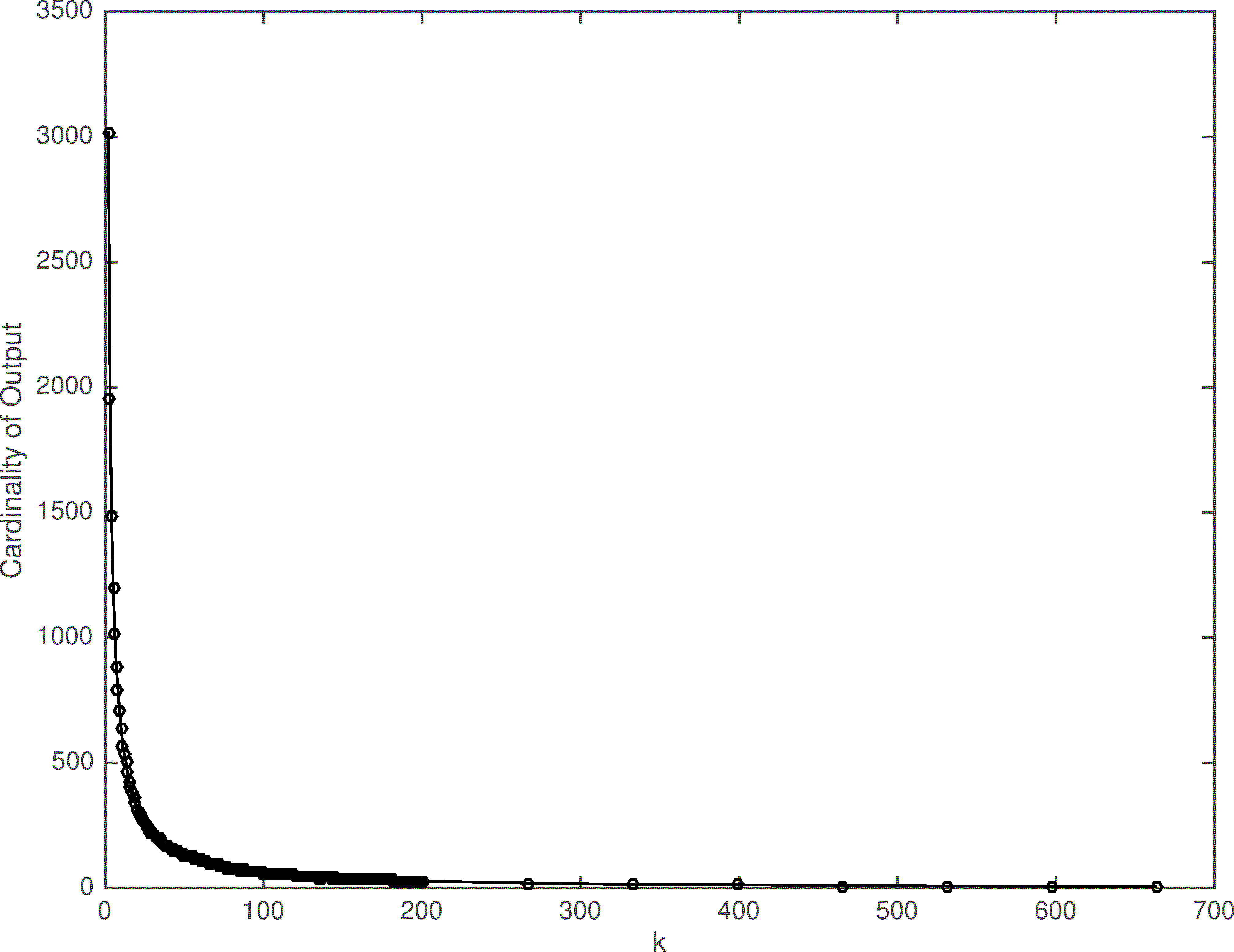
The introduction of the resample step allows us to solve this sparsity problem. If we were able to choose the right parameter $k$, we could simply sparsify and then resample to get a good output. One can hope that the huge drop in the left graph could be used to choose the parameter. However, the knowledge of the ground truth is needed to compute it, and estimating the Hausdorff distance between a set and the ground truth is impossible without some additional assumptions like the uniformity we use.

A second example is given in Figure 9. Here, the input data is obtained from a set of noisy GPS trajectories in the city of Berlin. In particular, given a set of trajectories (each modeled as polygonal curves), we first convert it to a density field by KDE (kernel density estimation). We then take the input as the set of grid points in 2D where every point is associated with a mass (density). Figure 9 (a) shows the heat-map of the density field where light color indicates high density and blue indicates low density. In (b) and (c), we show the outputs of Declutter algorithm (the ParfreeDeclutter algorithm would not provide good results as the input is highly non-uniform) for $k$ = 40 and $k=75$ respectively. In (d), we show the set of 40$\%$ points with the highest density values. The sampling of the road network is highly non-uniform. In particular, in the middle portion, even points off the roads have very high density (due to noisy input trajectories) as well. Hence a simple thresholding cannot remove these points and the output in (d) fills the space between roads in the middle portion. If we increase the threshold further, that is, reduce the number of points we want to keep in the thresholding, we will lose structures of some main roads. Our Declutter algorithm can capture the main road structures without collapsing nearby roads in the middle portion, although it also sparsifies the data.

(a)	(b)	(c)	(d)

Figure 9: (a)The heat-map of a density field generated from GPS traces. There are around 15k (weighted) grid points, serving as an input point set. The output of Algorithm Declutter when (b) $k=40$ and (c) $k=75$, (d) Thresholding of 40% points with the highest density.

Experiments on ParfreeDeclutter algorithm.

We will now illustrate our parameter-free denoising algorithm on several examples. Recall that the theoretical guarantee of the output of our parameter-free algorithm (i.e, ParfreeDeclutter algorithm) so far is only provided for samples satisfying some uniformity conditions.

We start with some curves in the plane. Figure 10 shows the results on two different inputs. In both cases, the curves have self-intersections. The noisy inputs are again obtained by moving every input point according to a Gaussian distribution and adding some white background noise. The details of the noise models can be found in Table 2 and the details on the size of the various point sets are given in Table 3.

The first steps of the algorithm remove the outliers lying further away from the ground truth. As the value of the parameter $k$ decreases, we remove nearby outliers. The result is a set of points located around the curves, in a tubular neighborhood of width that depends on the standard deviation of the Gaussian noise. Small sharp features are lost due to the blurring created by the Gaussian noise but the Hausdorff distance between the final output and the ground truth is as good as one can hope for when using a method oblivious of the ground truth.

Figure 10: Results of Algorithm ParfreeDeclutter on two samples of one dimensional compact sets. From left to right, the ground truth, the noisy input, two intermediate steps of the algorithm, and the final result.

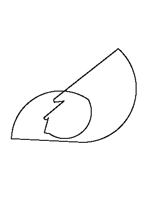
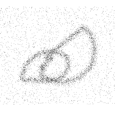
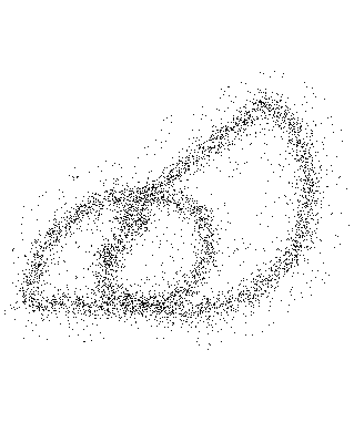
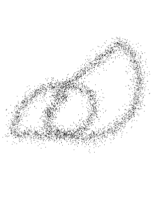
Figure 11 gives an example of an adaptive sample where Algorithm ParfreeDeclutter doesn’t work. The ground truth is a heptagon with its vertices being connected to the center. Algorithm ParfreeDeclutter doesn’t work in this case because the sample is highly non-uniform and the ambient noise is very dense (63.33% is ambient noise). The center part of the graph is significantly denser than other parts as the center vertex has a larger degree. So the sparser parts (other edges of the star and heptagon) are regarded as noises by Algorithm ParfreeDeclutter and thus removed.

Figure 11: A case where Algorithm ParfreeDeclutter doesn’t work. From left to right, the ground truth, the noisy input, an intermediate step of the algorithm and the final result.

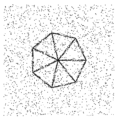
Figure 12 (Figure 5 in the main text) presents results obtained on an adaptive sample of a 2-manifold in 3D. We consider again the so-called Botijo example with an adaptive sampling. Contrary to the previous curves that were sampled uniformly, the density of this point set depends on the local feature size. We also generate the noisy input the same way, adding a Gaussian noise at each point that has a standard deviation proportional to the local feature size. Despite the absence of theoretical guarantees for the adaptive setting, Algorithm ParfreeDeclutter removes the outliers while maintaining the points close to the ground truth.

Figure 12: Experiment on a two dimensional manifold. From left to right, the ground truth, the noisy input, two intermediate steps of Algorithm ParfreeDeclutter and the final result.

Figure	Standard deviation of Gaussian	Size of ambient noise (percentage)
Figure 10 first row	0.05	2000 (37.99%)
Figure 10 second row	0.05	2000 (45.43%)
Figure 12	0.1	2000 (28.90%)

Table 2: Parameter of the noise model for Figure 10 and Figure 12

Figure	Sample	Ground truth	Noise input	Intermediate steps	Final result
Figure 10 first row	uniform	5264	7264	6026       5875	5480
Figure 10 second row	uniform	4402	6402	5197       4992	4475
Figure 12	adaptive	6921	8921	7815       7337	6983

Table 3: Cardinality of each dataset in Figure 10 and Figure 12

Finally, our last example is on a high dimensional data set. We use subsets of the MINIST database. This database contains handwritten digits. We take all ”1” digits (1000 images) and add some images from other digits to constitute the noise. Every image is a $28\times 28$ matrix and is considered as a point in dimension $784$. We then use the $L_{2}$ metric between the images. Table 4 contains our experiment result. Our algorithm partially removes the noisy points as well as a few good points. If we add some random points in our space, we no longer encounter this problem, which means if we add points with every pixel a random number, then we can remove all noises without removing any good points.

Ground truth	Noise	Images removed after sampling	Digit 1 removed
1000 digit 1	200 digit 7	85	5
1000 digit 1	200 digit 8	94	5
1000 digit 1	200 digit 0-9 except 1	126	9

Table 4: Experiment on high-dimension datasets. The third and forth columns show number of corresponding images.

Denoising for data classification.

Finally, we apply our denoising algorithm as a pre-processing for high-dimensional data classification. Specifically, here we use MNIST data sets, which is a database of handwritten digits from ’0’ to ’9’. Table 5 shows the experiment on digit 1 and digit 7. We take a random collection of 1352 images of digit ’1’ and 1279 images of digit ’7’ correctly labeled as training set, and take 10816 number of images of digit 1 and digit 7 as testing set. Each of the image is $28\times 28$ and thus can be viewed as a vector in $\mathbb{R}^{784}$. We use the $L_{1}$ metric to measure distance between such image-vectors. We use a linear SVM to classify the 10816 testing images. The classification error rate for the testing set is $0.6564\%$, shown in the second row of Table 5.

Next, we artificially add two types of noises to input data: the swapping-noise and the background-noise.

The swapping-noise means that we randomly mislabel some images of ‘1’ as ’7’, and some images of ‘7’ as ’1’. As shown in the third row of Table 5, the classification error increases to about $4.096\%$ after such mislabeling in the training set.

Next, we apply our ParfreeDeclutter algorithm to the training set (to the images with label ’1’ and those with label ’7’ separately) to first clean up the training set. As we can see in Row-6 of Table 5, we removed most images with a mislabeled ‘1’ which means the image is ’7’ but it is labeled as ’1’. We then use the denoised dataset as the training set, and improved the classification error to $2.45\%$.

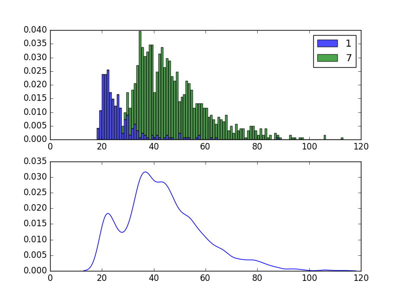
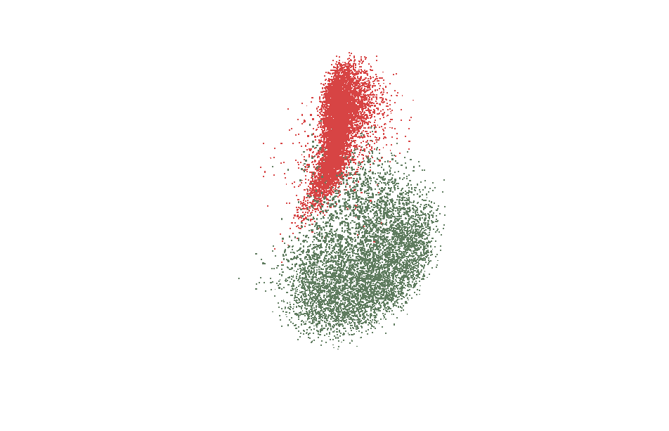
While our denoising algorithm improved the classification accuracy, we note that it does not remove many mislabeled ‘7’s from the set of images of digit ‘7’. The reason is that the images of ‘1’ are significantly more clustered than those of digit ‘7’. Hence the set of images of ‘1’s labelled as ‘7’ themselves actually form a cluster; those points actually have even smaller k-distance than the images of ‘7’ as shown in Figure 13, and thus are considered to be signal by our denoising algorithm.

Figure 13: Left: $k$-distance density distribution of digit 7s with digit 1s as the noise when $k=32$: Note, the points corresponding to images of digit ‘1’ actually have a smaller $k$-distance than those of digit ‘7’. Right: Graph after being reduced to 3 dimension by PCA, the red one is for 1s, the green one is for 7s.

The second type of noise is the background noise, where we replace the black backgrounds of a random subset of images in the training set (250 ‘1’s and 250 ‘7’s) with some other grey-scaled images. Under such noise, the classification error increases to $1.146\%$. Again, we perform our ParfreeDeclutter algorithm to the training set separately, and use the denoised data sets as the new training set. The classification error is then improved to $0.7488\%$.

1						Error(%)
2	Original	# Digit 1 1352		# Digit 7 1279		0.6564
3	Swap. Noise	# Mislabelled 1 270		# Mislabelled 7 266		4.0957
4		Digit 1		Digit 7
5		# Removed	# True Noise	# Removed	# True Noise
6	L1 Denoising	314	264	17	1	2.4500

7	Back. Noise	# Noisy 1 250		# Noisy 7 250		1.1464
8		Digit 1		Digit 7
9		# Removed	# True Noise	# Removed	# True Noise
10	L1 Denoising	294	250	277	250	0.7488

Table 5: Results of denoising on digit 1 and digit 7 from the MNIST.

References

- [1] N. Amenta and M. Bern. Surface reconstruction by voronoi filtering. Discr. Comput. Geom., 22:481–504, 1999.
- [2] G. Biau et al. A weighted k-nearest neighbor density estimate for geometric inference. Electronic Journal of Statistics, 5:204–237, 2011.
- [3] J.-D. Boissonnat, L. J. Guibas, and S. Y. Oudot. Manifold reconstruction in arbitrary dimensions using witness complexes. Discr. Comput. Geom., 42(1):37–70, 2009.
- [4] M. Buchet. Topological inference from measures. PhD thesis, Paris 11, 2014.
- [5] M. Buchet, F. Chazal, T. K. Dey, F. Fan, S. Y. Oudot, and Y. Wang. Topological analysis of scalar fields with outliers. In Proc. 31st Sympos. Comput. Geom., pages 827–841, 2015.
- [6] M. Buchet, F. Chazal, S. Y. Oudot, and D. R. Sheehy. Efficient and robust persistent homology for measures. In Proc. ACM-SIAM Sympos. Discr. Algo., pages 168–180, 2015.
- [7] C. Caillerie, F. Chazal, J. Dedecker, and B. Michel. Deconvolution for the wasserstein metric and geometric inference. In Geom. Sci. Info., pages 561–568. 2013.
- [8] T-H H. Chan, M. Dinitz, and A. Gupta. Spanners with slack. In Euro. Sympos. Algo., pages 196–207, 2006.
- [9] F. Chazal, D. Cohen-Steiner, and A. Lieutier. A sampling theory for compact sets in Euclidean space. Discr. Comput. Geom., 41(3):461–479, 2009.
- [10] F. Chazal, D. Cohen-Steiner, and Q. Mérigot. Geometric inference for probability measures. Found. Comput. Math., 11(6):733–751, 2011.
- [11] F. Chazal and S. Y. Oudot. Towards persistence-based reconstruction in Euclidean spaces. In Proc. 24th Sympos. Comput. Geom., pages 232–241, 2008.
- [12] D. Cohen-Steiner, H. Edelsbrunner, and J. Harer. Stability of persistence diagrams. Discr. Comput. Geom., 37(1):103–120, 2007.
- [13] D. Comaniciu and P. Meer. Mean shift: A robust approach toward feature space analysis. IEEE Trans. Pattern Anal. Machine Intelligence, 24(5):603–619, 2002.
- [14] T. K. Dey, Z. Dong, and Y. Wang. Parameter-free topology inference and sparsification for data on manifolds. In Proc. ACM-SIAM Sympos. Discr. Algo., pages 2733–2747, 2017.
- [15] T. K. Dey, J. Giesen, S. Goswami, and W. Zhao. Shape dimension and approximation from samples. Discr. Comput. Geom., 29:419–434, 2003.
- [16] D. L. Donoho. De-noising by soft-thresholding. IEEE Trans. Info. Theory., 41(3):613–627, 1995.
- [17] H. Edelsbrunner and J. Harer. Computational Topology: an Introduction. American Mathematical Soc., 2010.
- [18] C. R. Genovese et al. On the path density of a gradient field. The Annal. Statistics, 37(6A):3236–3271, 2009.
- [19] L. Guibas, D. Morozov, and Q. Mérigot. Witnessed k-distance. Discr. Comput. Geom., 49(1):22–45, 2013.
- [20] A. Hatcher. Algebraic Topology. Cambridge University Press, 2002.
- [21] V. J. Hodge and J. Austin. A survey of outlier detection methodologies. Artificial Intelligence Review, 22(2):85–126, 2004.
- [22] H. Jiang and S. Kpotufe. Modal-set estimation with an application to clustering. arXiv preprint arXiv:1606.04166, 2016.
- [23] A. Meister. Deconvolution problems in nonparametric statistics. Lecture Notes in Statistics. Springer, 2009.
- [24] J. R. Munkres. Elements of algebraic topology, volume 2. Addison-Wesley Reading, 1984.
- [25] U. Ozertem and D. Erdogmus. Locally defined principal curves and surfaces. J. Machine Learning Research, 12:1249–1286, 2011.
- [26] B. W. Silverman. Density estimation for statistics and data analysis, volume 26. CRC press, 1986.
- [27] J. Zhang. Advancements of outlier detection: A survey. EAI Endorsed Trans. Scalable Information Systems, 1(1):e2, 2013.