Deep multi-scale video prediction beyond mean square error
Abstract
Learning to predict future images from a video sequence involves the construction of an internal representation that models the image evolution accurately, and therefore, to some degree, its content and dynamics. This is why pixel-space video prediction may be viewed as a promising avenue for unsupervised feature learning. In addition, while optical flow has been a very studied problem in computer vision for a long time, future frame prediction is rarely approached. Still, many vision applications could benefit from the knowledge of the next frames of videos, that does not require the complexity of tracking every pixel trajectory. In this work, we train a convolutional network to generate future frames given an input sequence. To deal with the inherently blurry predictions obtained from the standard Mean Squared Error (MSE) loss function, we propose three different and complementary feature learning strategies: a multi-scale architecture, an adversarial training method, and an image gradient difference loss function. We compare our predictions to different published results based on recurrent neural networks on the UCF101 dataset.
1 Introduction
Unsupervised feature learning of video representations is a promising direction of research because the resources are quasi-unlimited and the progress remaining to achieve in this area are quite important. In this paper, we address the problem of frame prediction. A significant difference with the more classical problem of image reconstruction (Vincent et al., 2008; Le, 2013) is that the ability of a model to predict future frames requires to build accurate, non trivial internal representations, even in the absence of other constraints (such as sparsity). Therefore, we postulate that the better the predictions of such system are, the better the feature representation should be. Indeed, the work of Srivastava et al. (2015) demonstrates that learning representations by predicting the next sequence of image features improves classification results on two action recognition datasets. In this work, however, we focus on predicting directly in pixel space and try to address the inherent problems related to this approach.
Top performing algorithms for action recognition exploit the temporal information in a supervised way, such as the 3D convolutional network of Tran et al. (2015), or the spatio-temporal convolutional model of Simonyan & Zisserman (2014), which can require months of training, and heavily labeled datasets. This could be reduced using unsupervised learning. The authors in (Wang & Gupta, 2015) compete with supervised learning performance on ImageNet, by using a siamese architecture (Bromley et al., 1993) to mine positive and negative examples from patch triplets of videos in an unsupervised fashion. Unsupervised learning from video is also exploited in the work of Vondrick et al. (2015), where a convolutional model is trained to predict sets of future possible actions, or in (Jayaraman & Grauman, 2015) which focuses on learning a feature space equivariant to ego-motion. Goroshin et al. (2015) trained a convolutional network to learn to linearize motion in the code space and tested it on the NORB dataset. Beside unsupervised learning, a video predictive system may find applications in robotics (Kosaka & Kak, 1992), video compression (Ascenso et al., 2005) and inpainting (Flynn et al., 2015) to name a few.
Recently, predicting future video sequences appeared in different settings: Ranzato et al. (2014) defined a recurrent network architecture inspired from language modeling, predicting the frames in a discrete space of patch clusters. Srivastava et al. (2015) adapted a LSTM model (Hochreiter & Schmidhuber, 1997) to future frame prediction. Oh et al. (2015) defined an action conditional auto-encoder model to predict next frames of Atari-like games. In the two works dealing with natural images, a blur effect is observed in the predictions, due to different causes. In (Ranzato et al., 2014), the transformation back and forth between pixel and clustered spaces involves the averaging of 64 predictions of overlapping tilings of the image, in order to avoid a blockiness effect in the result. Short term results from Srivastava et al. (2015) are less blurry, however the loss function inherently produces blurry results. Indeed, using the loss comes from the assumption that the data is drawn from a Gaussian distribution, and works poorly with multimodal distributions.
In this work, we address the problem of lack of sharpness in the predictions. We assess different loss functions, show that generative adversarial training (Goodfellow et al., 2014; Denton et al., 2015) may be successfully employed for next frame prediction, and finally introduce a new loss based on the image gradients, designed to preserve the sharpness of the frames. Combining these two losses produces the most visually satisfying results.
Our paper is organised as follows: the model section describes the different model architectures: simple, multi-scale, adversarial, and presents our gradient difference loss function. The experimental section compares the proposed architectures and losses on video sequences from the Sports1m dataset of Karpathy et al. (2014) and UCF101 (Soomro et al., 2012). We further compare our results with (Srivastava et al., 2015) and (Ranzato et al., 2014). We measure the quality of image generation by computing similarity and sharpness measures.
2 Models
Let be a sequence of frames to predict from input frames in a video sequence. Our approach is based on a convolutional network (LeCun et al., 1998), alternating convolutions and Rectified Linear Units (ReLU) (Nair & Hinton, 2010).
| Input | First | Second | Third | Fourth | Fifth | Output |
|---|---|---|---|---|---|---|
| feature map | feature map | feature map | feature map | feature map |

conv. ReLU conv. ReLU conv. ReLU conv. ReLU conv. Tanh
Such a network , displayed in Figure 1, can be trained to predict one or several concatenated frames from the concatenated frames by minimizing a distance, for instance with or , between the predicted frame and the true frame:
| (1) |
However, such a network has at least two major flaws:
1. Convolutions only account for short-range dependencies, limited by the size of their
kernels. However, using pooling
would only be part of the solution since the output has to be of the same resolution as
the input. There are a number of ways to avoid the loss of resolution brought about by
pooling/subsampling while preserving long-range dependencies.
The simplest and oldest one is to have no pooling/subsampling but many convolution
layers (Jain et al., 2007).
Another method is to use connections that “skip” the pooling/unpooling pairs, to preserve
the high frequency information
(Long et al., 2015; Dosovitskiy et al., 2015; Ronneberger et al., 2015).
Finally, we can combine multiple scales linearly as in the reconstruction process of
a Laplacian pyramid (Denton et al., 2015). This is the approach we use in this paper.
2. Using an loss, and to a lesser extent , produces blurry predictions,
increasingly worse when predicting further in the future. If the probability distribution
for an output pixel has two equally likely modes and , the value
minimizes the loss over the data, even if has very low probability.
In the case of an norm, this effect diminishes, but do not disappear,
as the output value would be the median of the set of equally likely values.
2.1 Multi-scale network
We tackle Problem 1 by making the model multi-scale. A multi-scale version of the model is defined as follows: Let be the sizes of the inputs of our network. Typically, in our experiments, we set , , and . Let be the upscaling operator toward size . Let , denote the downscaled versions of and of size , and be a network that learns to predict from and a coarse guess of . We recursively define the network , that makes a prediction of size , by
| (2) |
Therefore, the network makes a series of predictions, starting from the lowest resolution, and uses the prediction of size as a starting point to make the prediction of size . At the lowest scale , the network takes only as an input. This architecture is illustrated on Figure 2, and the specific details are given in Section 3. The set of trainable parameters is denoted and the minimization is performed via Stochastic Gradient Descent (SGD).

Despite the multi-scale architecture, the search of from without making any assumption on the space of possible configurations still leads to blurry predictions, because of Problem 2. In order to further reduce this effect, the next two sections introduce an adversarial strategy and the image gradient difference loss.
2.2 Adversarial training
Generative adversarial networks were introduced by Goodfellow et al. (2014), where images patches are generated from random noise using two networks trained simultaneously. In that work, the authors propose to use a discriminative network to estimate the probability that a sample comes from the dataset instead of being produced by a generative model . The two models are simultaneously trained so that learns to generate frames that are hard to classify by , while learns to discriminate the frames generated by . Ideally, when is trained, it should not be possible for to perform better than chance.
We adapted this approach for the purpose of frame prediction, which constitutes to our knowledge the first application of adversarial training to video prediction. The generative model is typically the one described in the previous section. The discriminative model takes a sequence of frames, and is trained to predict the probability that the last frames of the sequence are generated by . Note only the last frames are either real of generated by , the rest of the sequence is always from the dataset. This allows the discriminative model to make use of temporal information, so that learns to produce sequences that are temporally coherent with its input. Since is conditioned on the input frames , there is variability in the input of the generator even in the absence of noise, so noise is not a necessity anymore. We trained the network with and without adding noise and did not observe any difference. The results we present are obtained without random noise.
Our main intuition on why to use an adversarial loss is that it can, theoretically, address the Problem 2 mentioned in Section 2. Imagine a sequence of frames for which, in the dataset, the next frames can either be or , with equal probability. As explained before, training the network with an loss will result in predicting the average frames . However, the sequence , composed of the frames of followed by the frames of , is not a likely sequence, and can discriminate them easily. The only sequences the model will not be able to classify as fake are and .
The discriminative model is a multi-scale convolutional network with a single scalar output. The training of the pair (, ) consists of two alternated steps, described below. For the sake of clarity, we assume that we use pure SGD (minibatches of size 1), but there is no difficulty to generalize the algorithm to minibatches of size M by summing the losses over the samples.
Training :
Let be a sample from the dataset. Note that (respectively ) is a sequence of (respectively ) frames. We train to classify the input into class and the input into class . More precisely, for each scale , we perform one SGD iteration of while keeping the weights of fixed. It is trained with in the target for the datapoint , and the target for . Therefore, the loss function we use to train is
| (3) |
where is the binary cross-entropy loss, defined as
| (4) |
where takes its values in and in .
Training :
Let be a different data sample. While keeping the weights of fixed, we perform one SGD step on to minimize the adversarial loss:
| (5) |
Minimizing this loss means that the generative model is making the discriminative model as “confused” as possible, in the sense that will not discriminate the prediction correctly. However, in practice, minimizing this loss alone can lead to instability. can always generate samples that “confuse” , without being close to . In turn, will learn to discriminate these samples, leading to generate other “confusing” samples, and so on. To address this problem, we train the generator with a combined loss composed of the of the adversarial loss and the loss . The generator is therefore trained to minimize . There is therefore a tradeoff to adjust, by the mean of the and parameters, between sharp predictions due to the adversarial principle, and similarity with the ground truth brought by the second term. This process is summarized in Algorithm 1, with minibatches of size .
2.3 Image Gradient Difference Loss (GDL)
Another strategy to sharpen the image prediction is to directly penalize the differences of image gradient predictions in the generative loss function. We define a new loss function, the Gradient Difference Loss (GDL), that can be combined with a and/or adversarial loss function. The GDL function between the ground truth image , and the prediction is given by
| (6) |
where is an integer greater or equal to 1, and denotes the absolute value function. To the best of our knowledge, the closest related work to this idea is the work of Mahendran & Vedaldi (2015), using a total variation regularization to generate images from learned features. Our GDL is fundamentally different: In (Mahendran & Vedaldi, 2015), the total variation takes only the reconstructed frame in input, whereas our loss penalises gradient differences between the prediction and the true output. Second, we chose the simplest possible image gradient by considering the neighbor pixel intensities differences, rather than adopting a more sophisticated norm on a larger neighborhood, for the sake of keeping the training time low.
2.4 Combining losses
In our experiments, we combine the losses previously defined with different weights. The final loss is:
| (7) |
3 Experiments
We now provide a quantitative evaluation of the quality of our video predictions on UCF101 (Soomro et al., 2012) and Sports1m (Karpathy et al., 2014) video clips. We train and compare two configurations: (1) We use input frames to predict one future frame. In order to generate further in the future, we apply the model recursively by using the newly generated frame as an input. (2) We use input frames to produce frames simultaneously. This second configuration represents a significantly harder problem and is presented in Appendix.
3.1 Datasets
We use the Sports1m for the training, because most of UCF101 frames only have a very small portion of the image actually moving, while the rest is just a fixed background. We train our network by randomly selecting temporal sequences of patches of pixels after making sure they show enough movement (quantified by the difference between the frames). The data patches are first normalized so that their values are comprised between -1 and 1.
3.2 Network architecture
| Generative network scales | ||||
|---|---|---|---|---|
| Number of feature maps | 128, 256, 128 | 128, 256, 128 | 128, 256, 512, 256, 128 | 128, 256, 512, 256, 128 |
| Conv. kernel size | 3, 3, 3, 3 | 5, 3, 3, 5 | 5, 3, 3, 3, 5 | 7, 5, 5, 5, 5, 7 |
| Adversarial network scales | ||||
| Number of feature maps | 64 | 64, 128, 128 | 128, 256, 256 | 128, 256, 512, 128 |
| Conv. kernel size (no padding) | 3 | 3, 3, 3 | 5, 5, 5 | 7, 7, 5, 5 |
| Fully connected | 512, 256 | 1024, 512 | 1024, 512 | 1024, 512 |
We present results for several models. Unless otherwise stated, we employed mutliscale architectures. Our baseline models are using and losses. The GDL- (respectively GDL-) model is using a combination of the GDL with (respectively ) and (respectively ) loss; the relative weights and are both . The adversarial (Adv) model uses the adversarial loss, with weighted by and . Finally, the Adv+GDL model is a combination or the adversarial loss and the GDL, with the same parameters as for Adv with and .
Generative model training:
The generative model architecture is presented in Table 1. It contains padded convolutions interlaced with ReLU non linearities. A Hyperbolic tangent (Tanh) is added at the end of the model to ensure that the output values are between -1 and 1. The learning rate starts at and is reduced over time to . The minibatch size is set to , or in the case of the adversarial training, to take advantage of GPU hardware capabilities. We train the network on small patches, and since it is fully convolutional, we can seamlessly apply it on larger images at test time.
Adversarial training:
The discriminative model , also presented in Table 1, uses standard non padded convolutions followed by fully connected layers and ReLU non linearities. For the largest scale , a pooling is added after the convolutions. The network is trained by setting the learning rate to .
3.3 Quantitative evaluations
To evaluate the quality of the image predictions resulting from the different tested systems, we compute the Peak Signal to Noise Ratio (PSNR) between the true frame and the prediction :
| (8) |
where is the maximum possible value of the image intensities. We also provide the Structural Similarity Index Measure (SSIM) of Wang et al. (2004). It ranges between -1 and 1, a larger score meaning a greater similarity between the two images.
To measure the loss of sharpness between the true frame and the prediction, we define the following sharpness measure based on the difference of gradients between two images and :
| (9) |
where and .
| frame prediction scores | frame prediction scores | |||||
|---|---|---|---|---|---|---|
| Similarity | Sharpness | Similarity | Sharpness | |||
| PSNR | SSIM | PSNR | SSIM | |||
| single sc. | 26.5 | 0.84 | 24.7 | 22.4 | 0.82 | 24.2 |
| 27.6 | 0.86 | 24.7 | 22.5 | 0.81 | 24.2 | |
| 28.7 | 0.88 | 24.8 | 23.8 | 0.83 | 24.3 | |
| GDL | 29.4 | 0.90 | 25.0 | 24.9 | 0.84 | 24.4 |
| GDL | 29.9 | 0.90 | 25.0 | 26.4 | 0.87 | 24.5 |
| Adv∗ | 30.6 | 0.89 | 25.2 | 26.1 | 0.85 | 24.2 |
| Adv+GDL∗ | 31.5 | 0.91 | 25.4 | 28.0 | 0.87 | 25.1 |
| Adv+GDL fine-tuned ∗ | 32.0 | 0.92 | 25.4 | 28.9 | 0.89 | 25.0 |
| Last input | 28.6 | 0.89 | 24.6 | 26.3 | 0.87 | 24.2 |
| Optical flow | 31.6 | 0.93 | 25.3 | 28.2 | 0.90 | 24.7 |
∗ models fine-tuned on patches of size .

| Target | Target | Adv+GDL | Adv+GDL | Masked | Masked | Masked | Masked |
| image 1 | image 2 | Pred. 1 | Pred. 2 | Target 1 | Target 2 | Pred. 1 | Pred. 2 |
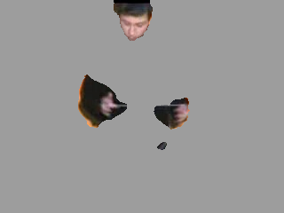
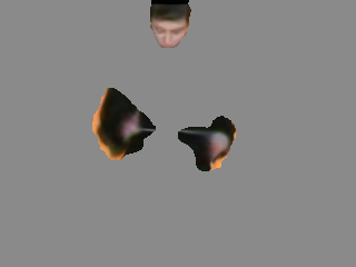
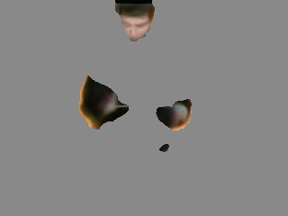
As for the other measures, a larger score is better. These quantitative measures on 378 test videos from UCF101111We extracted from the test set list video files every 10 videos, starting at 1, 11, 21 etc. are given in Table 2. As it is trivial to predict pixel values in static areas, especially on the UCF101 dataset where most of the images are still, we performed our evaluation in the moving areas as displayed in Figure 3. To this end, we use the EpicFlow method of Revaud et al. (2015), and compute the different quality measures only in the areas where the optical flow is higher than a fixed threshold 222We use default parameters for the Epic Flow computation, and transformed the .flo file to png using the Matlab code http://vision.middlebury.edu/flow/code/flow-code-matlab.zip. If at least one color channel is lower than 0.2 (image color range between 0 and 1), we replace the corresponding pixel intensity of the output and ground truth to 0, and compute similarity measures in the resulting masked images.. Similarity and sharpness measures computed on the whole images are given in Appendix.
The numbers clearly indicate that all strategies perform better than the predictions in terms of PSNR, SSIM and sharpness. The multi-scale model brings some improvement, but used with an norm, it does not outperform simple frame copy in the moving areas. The model improves the results, since it replaces the mean by the median value of individual pixel predictions. The GDL and adversarial predictions are leading to further gains, and finally the combination of the multi-scale, norm, GDL and adversarial training achieves the best PSNR, SSIM and Sharpness difference measure.
It is interesting to note that while we showed that the norm was a poor metric for training predictive models, the PSNR at test time is the worst for models trained optimising the norm, although the PSNR is based on the metric. We also include the baseline presented in Ranzato et al. (2014) – courtesy of Piotr Dollar – that extrapolates the pixels of the next frame by propagating the optical flow from the previous ones.
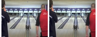
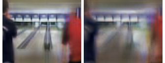
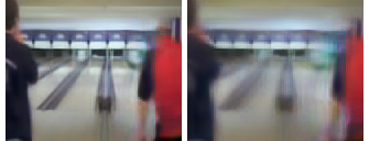
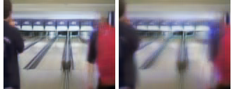
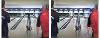
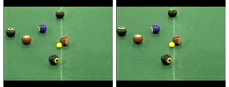
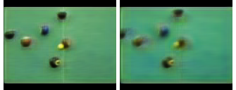
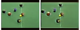
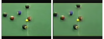
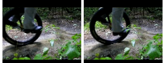
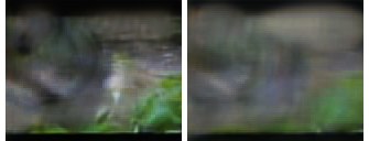
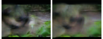
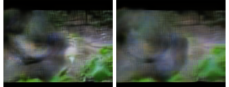
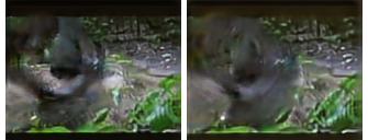
Figure 4 shows results on test sequences from the Sport1m dataset, as movements are more visible in this dataset.
 |
 |
 |
|
| Input frames | Ground truth | result | |
 |
 |
 |
 |
| result | GDL result | Adversarial result | Adversarial+GDL result |
 |
 |
 |
|
| Input frames | Ground truth | result | |
 |
 |
 |
 |
| result | GDL result | Adversarial result | Adversarial+GDL result |
 |
 |
 |
|
| Input frames | Ground truth | result | |
 |
 |
 |
 |
| result | GDL result | Adversarial result | Adversarial+GDL result |
3.4 Comparison to Ranzato et al. (2014)
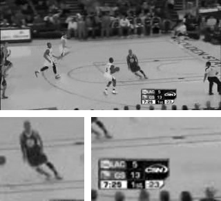
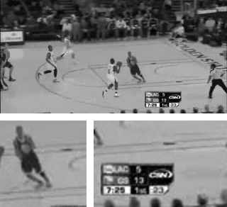
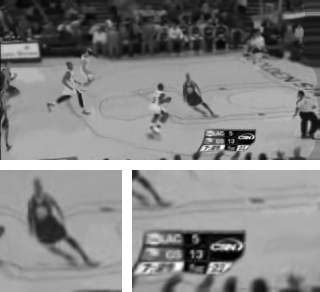
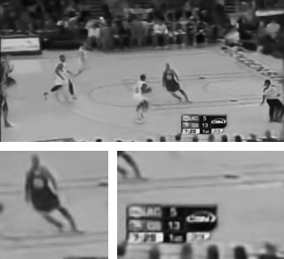
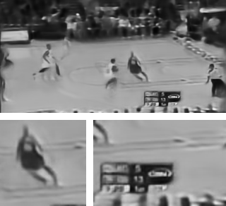
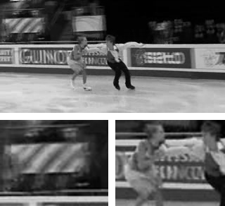
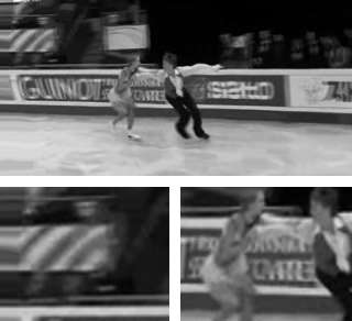
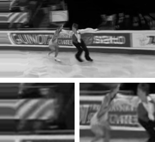
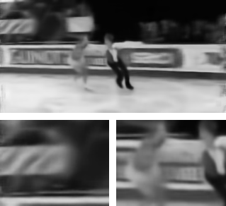
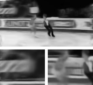
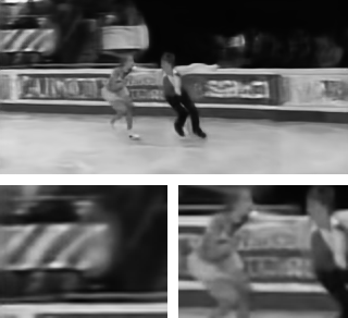
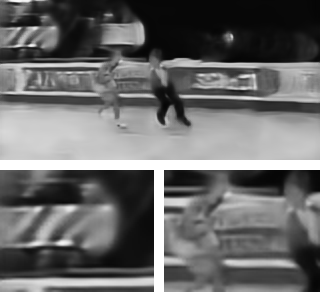
In this section, we compare our results to (Ranzato et al., 2014). To obtain grayscale images, we make RGB predictions and extract the Y channel of our Adv+GDL model. Ranzato et al. (2014) images are generated by averaging 64 results obtained using different tiling to avoid a blockiness effect, however creating instead a blurriness effect. We compare the PSNR and SSIM values on the first predicted images of Figure 5.
|

|
|---|---|
| Target | Prediction using a constant optical flow |
| PSNR = 25.4 (18.9), SSIM = 0.88 (0.56) |

|
|
|---|---|
| Ranzato et al. result | Adv GDL result |
| PSNR = 16.3 (15.1), SSIM = 0.70 (0.55) | PSNR = 26.7 (19.0), SSIM = 0.89 (0.59) |
|
|
|---|---|
| Target | Prediction using a constant optical flow |
| PSNR = 24.7 (20.6), SSIM = 0.84 (0.72) |
|
|
|---|---|
| Ranzato et al. result | Adv GDL result |
| PSNR = 20.1 (17.8), SSIM = 0.72 (0.65) | PSNR = 24.6 (20.5), SSIM = 0.81 (0.69) |
We note that the results of Ranzato et al. appear slightly lighter than our results because of a normalization that does not take place in the original images, therefore the errors given here are not reflecting the full capacity of their approach. We tried to apply the blind deconvolution method of Krishnan et al. (2011) to improve Ranzato et al. and our different results. As expected, the obtained sharpness scores are higher, but the image similarity measures are deteriorated because often the contours of the predictions do not match exactly the targets. More importantly, Ranzato et al. results appear to be more static in moving areas. Visually, the optical flow result appears similar to the target, but a closer look at thin details reveals that lines, heads of people are bent or squeezed.
4 Conclusion
We provided a benchmark of several strategies for next frame prediction, by evaluating the quality of the prediction in terms of Peak Signal to Noise Ratio, Structural Similarity Index Measure and image sharpness. We display our results on small UCF video clips at http://cs.nyu.edu/~mathieu/iclr2016.html. The presented architectures and losses may be used as building blocks for more sophisticated prediction models, involving memory and recurrence. Unlike most optical flow algorithms, the model is fully differentiable, so it can be fine-tuned for another task if necessary. Future work will deal with the evaluation of the classification performances of the learned representations in a weakly supervised context, for instance on the UCF101 dataset. Another extension of this work could be the combination of the current system with optical flow predictions. Alternatively, we could replace optical flow predictions in applications that does not explicitly require optical flow but rather next frame predictions. A simple example is causal (where the next frame is unknown) segmentation of video streams.
Acknowledgments
We thank Florent Perronnin for fruitful discussions, and Nitish Srivastava, Marc’Aurelio Ranzato and Piotr Dollár for providing us their results on some video sequences.
References
- Ascenso et al. (2005) Ascenso, Joao, Brites, Catarina, and Pereira, Fernando. Improving frame interpolation with spatial motion smoothing for pixel domain distributed video coding. In 5th EURASIP Conference on Speech and Image Processing, Multimedia Communications and Services, pp. 1–6, 2005.
- Bromley et al. (1993) Bromley, Jane, Bentz, James W, Bottou, Léon, Guyon, Isabelle, LeCun, Yann, Moore, Cliff, Säckinger, Eduard, and Shah, Roopak. Signature verification using a “siamese” time delay neural network. Int. Journal of Pattern Recognition and Artificial Intelligence, 7(04):669–688, 1993.
- Denton et al. (2015) Denton, Emily, Chintala, Soumith, Szlam, Arthur, and Fergus, Rob. Deep generative image models using a laplacian pyramid of adversarial networks. In NIPS, 2015.
- Dosovitskiy et al. (2015) Dosovitskiy, Alexey, Springenberg, Jost Tobias, and Brox, Thomas. Learning to generate chairs with convolutional neural networks. In CVPR, 2015.
- Flynn et al. (2015) Flynn, John, Neulander, Ivan, Philbin, James, and Snavely, Noah. Deepstereo: Learning to predict new views from the world’s imagery. CoRR, abs/1506.06825, 2015.
- Goodfellow et al. (2014) Goodfellow, Ian J., Pouget-Abadie, Jean, Mirza, Mehdi, Xu, Bing, Warde-Farley, David, Ozair, Sherjil, Courville, Aaron C., and Bengio, Yoshua. Generative adversarial networks. NIPS, 2014.
- Goroshin et al. (2015) Goroshin, Ross, Mathieu, Michaël, and LeCun, Yann. Learning to linearize under uncertainty. NIPS, 2015.
- Hochreiter & Schmidhuber (1997) Hochreiter, Sepp and Schmidhuber, Jürgen. Long short-term memory. Neural Comput., 9(8):1735–1780, November 1997.
- Jain et al. (2007) Jain, Viren, Murray, Joseph F, Roth, Fabian, Turaga, Srinivas, Zhigulin, Valentin, Briggman, Kevin L, N, Helmstaedter Moritz, Denk, Winfried, and Seung, Sebastian H. Supervised learning of image restoration with convolutional networks. 2007.
- Jayaraman & Grauman (2015) Jayaraman, Dinesh and Grauman, Kristen. Learning image representations equivariant to ego-motion. In ICCV, 2015.
- Karpathy et al. (2014) Karpathy, Andrej, Toderici, George, Shetty, Sanketh, Leung, Thomas, Sukthankar, Rahul, and Fei-Fei, Li. Large-scale video classification with convolutional neural networks. In CVPR, 2014.
- Kosaka & Kak (1992) Kosaka, Akio and Kak, Avinash C. Fast vision-guided mobile robot navigation using model-based reasoning and prediction of uncertainties. CVGIP: Image understanding, 56(3):271–329, 1992.
- Krishnan et al. (2011) Krishnan, Dilip, Tay, Terence, and Fergus, Rob. Blind deconvolution using a normalized sparsity measure. In CVPR, pp. 233–240, 2011.
- Le (2013) Le, Quoc V. Building high-level features using large scale unsupervised learning. In ICASSP, pp. 8595–8598, 2013.
- LeCun et al. (1998) LeCun, Yann, Bottou, Léon, Bengio, Yoshua, and Haffner, Patrick. Gradient-based learning applied to document recognition. Proceedings of the IEEE, 86(11):2278–2324, 1998.
- Long et al. (2015) Long, Jonathan, Shelhamer, Evan, and Darrell, Trevor. Fully convolutional networks for semantic segmentation. In CVPR, 2015.
- Mahendran & Vedaldi (2015) Mahendran, Aravindh and Vedaldi, Andrea. Understanding deep image representations by inverting them. In CVPR, 2015.
- Nair & Hinton (2010) Nair, Vinod and Hinton, Geoffrey E. Rectified linear units improve restricted boltzmann machines. In ICML, pp. 807–814, 2010.
- Oh et al. (2015) Oh, Junhyuk, Guo, Xiaoxiao, Lee, Honglak, Lewis, Richard L., and Singh, Satinder P. Action-conditional video prediction using deep networks in atari games. NIPS, 2015.
- Ranzato et al. (2014) Ranzato, Marc’Aurelio, Szlam, Arthur, Bruna, Joan, Mathieu, Michaël, Collobert, Ronan, and Chopra, Sumit. Video (language) modeling: a baseline for generative models of natural videos. CoRR, abs/1412.6604, 2014.
- Revaud et al. (2015) Revaud, Jerome, Weinzaepfel, Philippe, Harchaoui, Zaid, and Schmid, Cordelia. EpicFlow: Edge-Preserving Interpolation of Correspondences for Optical Flow. In Computer Vision and Pattern Recognition, 2015.
- Ronneberger et al. (2015) Ronneberger, Olaf, Fischer, Philipp, and Brox, Thomas. U-net: Convolutional networks for biomedical image segmentation. In MICCAI, volume 9351, pp. 234–241. 2015.
- Simonyan & Zisserman (2014) Simonyan, Karen and Zisserman, Andrew. Two-stream convolutional networks for action recognition in videos. In NIPS, 2014.
- Soomro et al. (2012) Soomro, Khurram, Zamir, Amir Roshan, and Shah, Mubarak. UCF101: A dataset of 101 human actions classes from videos in the wild. CoRR, abs/1212.0402, 2012.
- Srivastava et al. (2015) Srivastava, Nitish, Mansimov, Elman, and Salakhutdinov, Ruslan. Unsupervised learning of video representations using LSTMs. In ICML, 2015.
- Tran et al. (2015) Tran, Du, Bourdev, Lubomir D., Fergus, Rob, Torresani, Lorenzo, and Paluri, Manohar. C3D: generic features for video analysis. In ICCV, 2015.
- Vincent et al. (2008) Vincent, Pascal, Larochelle, Hugo, Bengio, Yoshua, and Manzagol, Pierre-Antoine. Extracting and composing robust features with denoising autoencoders. In ICML, pp. 1096–1103. ACM, 2008.
- Vondrick et al. (2015) Vondrick, Carl, Pirsiavash, Hamed, and Torralba, Antonio. Anticipating the future by watching unlabeled video. CoRR, abs/1504.08023, 2015.
- Wang & Gupta (2015) Wang, Xiaolong and Gupta, Abhinav. Unsupervised learning of visual representations using videos. In ICCV, 2015.
- Wang et al. (2004) Wang, Zhou, Bovik, Alan C., Sheikh, Hamid R., and Simoncelli, Eero P. Image quality assessment: From error visibility to structural similarity. IEEE Trans. on Im. Proc., 13(4):600–612, 2004.
5 Appendix
5.1 Predicting the eight next frames
In this section, we trained our different multi-scale models – architecture described in Table 3– with input frames to predict frames simultaneously. Image similarity measures are given between the ground truth and the predictions in Table 4.
Models 8 frames in input – 8 frames in output
Generative network scales
Number of feature maps
16, 32, 64
16, 32, 64
32, 64, 128
32, 64, 128, 128
Conv. kernel size
3, 3, 3, 3
5, 3, 3, 3
5, 5, 5, 5
7, 5, 5, 5, 5
Adversarial network scales
Number of feature maps
16
16, 32, 32
32, 64, 64
32, 64, 128,
128
Conv. kernel size (no padding)
3
3, 3, 3
5, 5, 5
7, 7, 5, 5
Fully connected
128, 64
256, 128
256, 128
256, 128
For the first and eighth predicted frames, the numbers clearly indicate that all strategies perform better than the predictions in terms of PSNR and sharpness. The model, by replacing the mean intensity by the median value in individual pixel predictions, allows us to improve results. The adversarial predictions are leading to further gains, and finaly the GDL allows the predictions to achieve the best PNSR and sharpness. We note that the size of the network employed in the simultaneous prediction configuration is smaller than in the unique frame prediction setting.
| frame prediction scores | frame prediction scores | |||||
| Similarity | Sharpness | Similarity | Sharpness | |||
| PSNR | SSIM | PSNR | SSIM | |||
| 18.3 | 0.59 | 17.5 | 15.4 | 0.51 | 17.4 | |
| Adv | 21.1 | 0.61 | 17.6 | 17.1 | 0.52 | 17.4 |
| 21.3 | 0.66 | 17.7 | 17.0 | 0.55 | 17.5 | |
| GDL | 21.4 | 0.69 | 17.9 | 17.7 | 0.58 | 17.5 |
| Last input | 30.6 | 0.90 | 22.3 | 21.0 | 0.74 | 18.5 |
Figure 6 shows a generation result of eight frames simultaneously, using a large version of the GDL model in which all the number of feature maps were multiplied by four.


Compared to the recursive frame prediction as employed in the rest of the paper, predicting several input simultaneouly leads to better long term results but worst shorter term ones. The gap between the two performances could be reduced by the design of time multi-scale strategies.
5.2 Comparison to the LSTM approach of Srivastava et al. (2015)
Figure 7 shows a comparison with predictions based on LSTMs using sequences of patches from (Srivastava et al., 2015). The model ranking established on UCF101 in terms of sharpness and PSNR remains unchanged on the two sequences. When we employ the setting 8 inputs-8 output described in Table 3, we note that the LSTM first frame prediction is sharper than our models predictions, however when looking at a longer term future, our gradient difference loss leads to sharper results. Comparing visually the GDL and GDL , we notice that the predictions suffer from a chessboard effect in the case. On the other hand, when employing the recursive strategy (4 inputs, 1 output), the adversarial training lead to much sharper predictions. It does not look like anything close to the ground truth on the long term, but it remains realistic.
| Input | ||
| Ground truth | ||
| LSTM 2048 | ||
| LSTM 4096 | ||
| GDL | ||
| GDL | ||
| Adversarial | ||
| Adv. recursive | ||
| Adv. rec. + GDL | ||
| GDL recursive | ||
| rec. | ||
| rec. |
5.3 Additional results on the UCF101 dataset
We trained the model described in Table 1 with our different losses to predict 1 frame from the 4 previous ones. We provide in Table 5 similarity (PSNR and SSIM) and sharpness measures between the different tested models predictions and frame to predict. The evaluation is performed on the full images but is not really meaningful because predicting the future location of static pixels is most accurately done by copying the last input frame.
| frame prediction scores | frame prediction scores | |||||
| Similarity | Sharpness | Similarity | Sharpness | |||
| PSNR | SSIM | PSNR | SSIM | |||
| single sc. | 19.0 | 0.59 | 17.8 | 14.2 | 0.48 | 17.5 |
| 20.1 | 0.64 | 17.8 | 14.1 | 0.50 | 17.4 | |
| 22.3 | 0.74 | 18.5 | 16.0 | 0.56 | 17.6 | |
| GDL | 23.9 | 0.80 | 18.7 | 18.6 | 0.64 | 17.7 |
| Adv | 24.4 | 0.77 | 18.7 | 18.9 | 0.59 | 17.3 |
| Adv+GDL | 27.2 | 0.83 | 19.6 | 22.6 | 0.72 | 18.5 |
| Adv+GDL fine-tuned | 29.6 | 0.90 | 20.3 | 26.0 | 0.83 | 19.4 |
| Last input | 30.0 | 0.90 | 22.1 | 25.8 | 0.84 | 20.3 |