Search for Compensated Isocurvature Perturbations with Planck Power Spectra
Abstract
In the standard inflationary scenario, primordial perturbations are adiabatic. The amplitudes of most types of isocurvature perturbations are generally constrained by current data to be small. If, however, there is a baryon-density perturbation that is compensated by a dark-matter perturbation in such a way that the total matter density is unperturbed, then this compensated isocurvature perturbation (CIP) has no observable consequence in the cosmic microwave background (CMB) at linear order in the CIP amplitude. Here we search for the effects of CIPs on CMB power spectra to quadratic order in the CIP amplitude. An analysis of the Planck temperature data leads to an upper bound , at the 68% confidence level, to the variance of the CIP amplitude. This is then strengthened to if Planck small-angle polarization data are included. A cosmic-variance-limited CMB experiment could improve the sensitivity to CIPs to . It is also found that adding CIPs to the standard CDM model can improve the fit of the observed smoothing of CMB acoustic peaks just as much as adding a non-standard lensing amplitude.
pacs:
98.70.Vc,95.35.+d,98.80.Cq,98.80.-kI Introduction
Cosmological density perturbations are thought to have their origin during inflation Mukhanov:1985rz ; astro-ph/0504097 ; Bardeen:1983qw . These perturbations seed the large-scale inhomogeneities that later grow to become galaxies and clusters astro-ph/9506072 . From structure formation and cosmic-microwave-background (CMB) observations, we know that primordial density perturbations have amplitude 1502.01589 .
Primordial perturbations can be classified into two groups depending on their initial conditions. Adiabatic perturbations are perturbations to the total energy density that leave the ratios of the different constituents of matter everywhere the same. Isocurvature perturbations involve perturbations to the relative number densities of different components of matter Peebles:1970ag ; astro-ph/9610219 ; astro-ph/0009131 ; astro-ph/9809142 . The simplest inflationary models have purely adiabatic fluctuations, while isocurvature fluctuations usually signal the presence of a second field during inflation, as in curvaton models hep-ph/0110002 ; astro-ph/0208055 .
Isocurvature perturbations between photons and a single other species are in general well constrained astro-ph/0409326 ; astro-ph/0509209 ; 0705.2853 . If, however, there is a baryon-density perturbation that is compensated by a dark-matter perturbation in such a way that the total matter density remains constant, then there are no pressure or gravitational-potential perturbations above the baryonic Jeans scale. These compensated isocurvature perturbations (CIPs) thus have no observable effect on the CMB at linear order in the CIP amplitude astro-ph/0212248 ; 0907.5400 . There are constraints from other observables, but these are a factor of weaker than the adiabatic component 0907.3919 ; 1107.5047 ; 1107.1716 ; 1306.4319 .
In the standard scenario, the CMB power spectrum is determined given fixed values of the baryon and dark-matter densities and , respectively, in units of the critical density. CIPs, however, introduce variations to and between different patches of the CMB sky. They thus induce a variation in the power spectrum from one patch of sky to another.
The mean power spectrum—that obtained by measurements over the entire sky—remains unaltered, to linear order in the CIP amplitude. The variations show up, however, in two different ways. First of all, the spatial modulation of the power spectrum is characterized by a departure from gaussianity, a specific nontrivial four-point function, or trispectrum. A search for such a trispectrum was performed in Ref. 1306.4319 . The second consequence, however, is a change to the power spectrum that arises to quadratic order in the CIP amplitude, which can be understood heuristically as a smoothing of features in the CMB power spectrum when different power spectra are averaged.
In this paper we seek this effect of CIPs on the CMB power spectra obtained by Planck. We parametrize the magnitude of the effect of CIPs in terms of an rms CIP amplitude . We find from a temperature-only analysis a constraint of , which is competitive with, and complements, that obtained from the complete trispectrum, although with a far simpler analysis. That figure improves to if Planck polarization data are included. We then make CIP sensitivity forecasts for future experiments. We also show that CIPs have a very similar effect on the power spectrum to changing the lensing amplitude . They can thus alleviate the tension between the lensing amplitude obtained from the Planck spectrum () and that expected from theory () 1502.01589 .
This paper is structured as follows. In Section II we review the physics of CIPs and their effects on the CMB power spectra. Then, in Section III we find a linear basis of estimators for CMB observables, including CIPs. In Section IV we apply our analysis to current CMB data and an ideal cosmic-variance-limited CMB experiment. We conclude in Section V.
II Compensated Isocurvature Perturbations
CIPs change the baryon and dark-matter densities in such a way that the total matter energy density, , remains unaltered. We parametrize their effect as
| (1) |
where and are the baryon and dark-matter energy densities respectively, the overbar represents their unperturbed values, and is the amplitude of the CIP in the specific direction at recombination. This expression is accurate for CIPs of sufficiently large angular scale, where they can be treated as a modulation of background parameters 1505.00639 .
The linear-order effects of CIPs are on scales at which the baryons behave differently from dark matter, corresponding to angular scales 1107.5047 , which makes them unobservable in the CMB, although potentially detectable using cosmological 21-cm absorption measurements at high redshift 0907.5400 . CIPs will also have consequences for the CMB fluctuations induced by adiabatic perturbations. In a region of high (high baryon density), decoupling will be longer, thereby smoothing the peak structure in the CMB power spectrum. The mean-free path of CMB photons would be reduced by the higher electron density, leading to less damping of CMB fluctuations on small angular scales. A higher baryon density also decreases the plasma sound speed and hence decreases the sound horizon at recombination Peebles:1970ag .
II.1 Angular properties
We expand the amplitude of the compensated isocurvature perturbations in spherical harmonics as
| (2) |
where the spherical-harmonic coefficients are statistically independent and have a variance given by
| (3) |
We take the ansatz of a scale-invariant power spectrum for in -space. For , this creates a scale-invariant angular power spectrum when projected onto the last-scattering surface (LSS), where is a dimensionless amplitude 1107.5047 . The simple picture of CIPs as a modulation of background parameters corresponds to a separate universe approximation, which was shown in Ref. 1505.00639 to only be valid for , as the imprint of CIPs are washed for at smaller CIP angular scales. We thus restrict our analysis to .
We assume that the CIP amplitude is a Gaussian random variable with zero average and variance . Instead of finding an estimator for each we will directly measure its variance, which can be expressed in terms of the CIP angular power spectrum as
| (4) |
which means that our constraints will be on the total power in CIPs and not on each individual . By using Eq. (4) we can relate the CIP variance to the amplitude of the power spectrum as,
| (5) |
II.2 Previous constraints
As CIPs do not change CMB power spectra at linear order, past work has relied on other observables to constrain their amplitude. For example, measurements of galaxy-cluster baryon fractions (obtained through X-ray observations) were used in Ref. 0907.3919 to search for CIPs, imposing the constraint . This technique, however, relies on clusters being fair samples of the baryon density in the universe, as well as being kinematically relaxed.
In Ref. 1107.5047 , the off-diagonal correlations in the CMB created by CIPs were computed, and a forecast was made of the sensitivities that could be reached by studying them with different instrumental setups. Data from the WMAP mission 1212.5226 were analyzed in Ref. 1306.4319 to constrain the amplitude of the CIP power spectrum to be smaller than at 68% C.L., which translates to a constraint on the CIP variance of , where the mode has been ignored due to reconstruction uncertainties.
II.3 Effect on the power spectrum
In our picture we treat the CIP amplitude as a Gaussian random variable. This allows us to calculate the observed CMB angular power spectrum by averaging over the CIP amplitudes,
| (6) |
which to first non-zero order in is given by
| (7) |
We calculate the second derivative by fitting near , as a function of . We have checked that terms that are higher order in are negligible for the upper limits to that we infer.
III CIP Estimators
We have shown expressions for how CIPs alter CMB power spectra. Now we consider how to estimate with measurements of the three main CMB power spectra, , , and . For that we use a Fisher-matrix analysis to fully capture the correlations between the CIP variance, , and the usual cosmological parameters.
Let us begin by reviewing the basics of linear (Fisher) cosmological-parameter estimation.
III.1 Linear estimators
Codes like CosmoMC astro-ph/0205436 and Python Monte Carlo 1210.7183 are commonly used for parameter analysis. It is, however, a computationally costly procedure. We already have a best fit for the six CDM model parameters in the absence of CIPs 1502.01589 , so we can perturb the model around this best fit by adding CIPs, increasing the number of parameters to seven. In that case the new best-fit parameters will not be too far away in parameter space from the old ones, so we can perform a linear analysis.
We construct a linear estimator of the parameters near their current best-fit values 1502.01589 . To do so we parametrize the power spectra as,
| (8) |
where is the best-fit (lensed) power spectrum, with . We have left out other CMB observables, such as B-mode polarization, due to the absence of sufficiently sensitive and foreground-free CMB polarization data. These could potentially have significant constraining power 0907.3919 ; 1107.5047 .
We define the first six original amplitudes to be the CDM parameters as , where and are the baryon and cold-dark-matter physical densities, is the tilt of the scalar power spectrum, and its amplitude. Here, is the optical depth of reionization and is the Hubble parameter. We define the deviations of these parameters from their best-fit values to be .
The basis functions for 6 are constructed as
| (9) |
where the derivatives are taken by fitting in CAMB astro-ph/9911177 near the best-fit values of the six CDM parameters.
Since we are going to add CIPs we will have , unless otherwise specified. The change in the power spectrum when adding CIPs is parametrized by Eq. (7), from where we can extract the seventh basis function
| (10) |
where the derivative is calculated in the separate-universe approximation, and has associated amplitude .
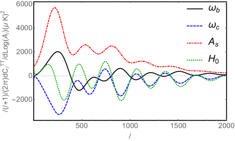
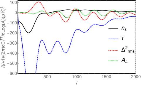
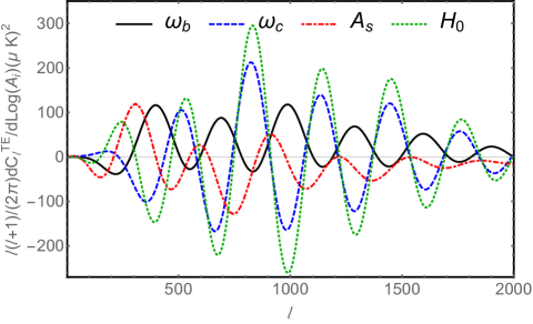
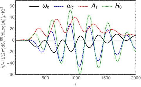
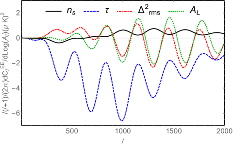
We show all the derivatives in Figures 1, 2, and 3. There are well-known correlations between the high- effects of changing the dark-matter density and the Hubble parameter . Similarly, increasing and decreasing produce very similar changes in the power spectra, except at the lowest s.
Notice that in those plots we are also showing the derivative with respect to the lensing amplitude as an eighth parameter. The basis functions for CIPs and lensing are very similar. This could help resolve the tension between the observed level of CMB lensing in Planck power spectra and expectations from the CDM model. We will explore this topic in Section IV.
III.2 Fisher Matrix
We now study the detectability of the seven simultaneously through a Fisher analysis. We employ the usual definition of the Fisher matrix Jungman:1995bz ; astro-ph/9603021 ; 1403.5271 , with components
| (11) |
where the inner product is defined as
| (12) |
The covariance matrix is given by astro-ph/9611125 ; astro-ph/9609170
| (13) |
where we have defined
| (14) |
and the are the instrumental noises, for which we use the Planck tabulated noise for the Planck analysis and zero in the cosmic-variance-limited case.
IV CMB analysis
Now we are ready to find estimates and errors for the six standard cosmological parameters, as well as the CIP amplitude .
We consider two cases. First, for Planck, we not only obtain estimators for the CIP variance, but also apply them to the data to obtain actual limits to CIPs. We will take a small detour to study the viability of CIPs as a solution for the lensing tension in the Planck CMB power spectra. Second, we will study a cosmic-variance limited (CVL) experiment.
IV.1 Planck constraint
Let us begin by considering the Planck 2015 power spectra (), obtained from the Planck Legacy Archive111http://pla.esac.esa.int/pla/. To diminish the effects of correlations between different s, we used binned data for , with width . The minimum-variance unbiased estimators for these seven amplitudes are
| (15) |
where is the inverse of the Fisher matrix, and is the residual after subtracting the best fit from the data, .
With the current data in the Planck Legacy Archive, however, it is hard to disentangle the optical depth and the scalar amplitude , since the effect of changing either is highly degenerate Bond:1987ub . The main difference between and is the reionization bump, caused by , that appears at low in polarization measurements Ng:1994sv ; astro-ph/9608050 ; astro-ph/0302404 . Our linear analysis underestimates the errors when using low- polarization data, so in lieu of them we will add a prior to the optical depth for robustness. We choose the final ranges to be for TT, and for TE and EE power spectra, where the maximum is that available in the Planck Legacy Archive. Later on, when considering lensing, we will add the full low- data to the analysis.
We show the best fits derived with this analysis in Table 1. The best fit to the CIP amplitude with TT-data only is , and with the combined data set is . There is thus no evidence for the existence of CIPs, and the constraint is of the same order of magnitude as the trispectrum constraint of Ref. 1306.4319 . Notice that we have not required to be positive. Imposing a prior would change the 68%C.L. constraints to for TT, for TE, for EE, and for the combined data set. Notice that these limits have become more constringent in the case of the TE data set, due to the negative best-fit value for , whereas the opposite is true for the TT and EE data sets.
| Parameter | TT | TE | EE | Combined |
|---|---|---|---|---|
| 0.022380.00028 | 0.021750.00052 | 0.02510.0015 | 0.022430.00017 | |
| 0.11930.0026 | 0.12170.0033 | 0.11120.0055 | 0.11940.0015 | |
| 0.96530.0081 | 0.9390.023 | 0.9860.018 | 0.96200.0049 | |
| 3.0970.036 | 3.080.040 | 3.110.040 | 3.110.034 | |
| 0.0820.018 | 0.0800.019 | 0.0780.019 | 0.0880.017 | |
| 67.71.3 | 66.01.7 | 72.13.1 | 67.40.71 | |
| 0.00580.0071 | 0.0230.020 | 0.0400.023 | 0.00090.0050 |
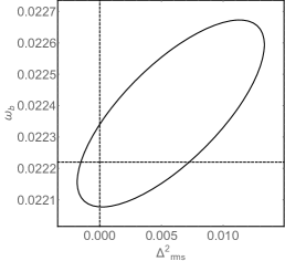
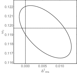
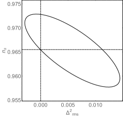
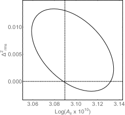
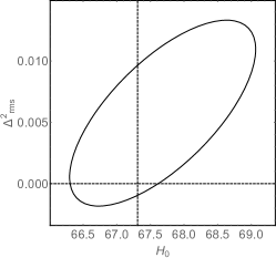
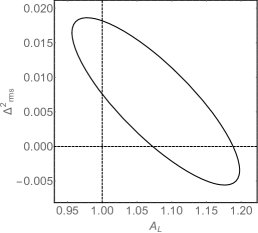
We show the confidence ellipses for the Planck experiment on Figures 4 and 5, where it is clear that the CIP contribution to the CMB power spectrum is highly correlated with most of the rest of parameters. The correlation coefficients, defined as , are found to be , , , , and .
We do not show the covariance between and , since the prior applied to renders meaningless the correlation coefficients. Even though this high- analysis shows no strong evidence for the existence of CIPs, they have the potential to resolve the lensing tension mentioned above, when including low- data. We now explore this possibility.
Lensing
The CMB is lensed by large-scale structure along the line of sight. The main effects of the lensing on the CMB power spectra are to add power at small scales and to smooth the acoustic peaks astro-ph/0601594 ; 1502.01591 . The amount of lensing inferred from CMB TT measurements seems, however, to be higher (by about two standard deviations) than the predicted value. This difference is parametrized through the lensing amplitude 0803.2309 ; astro-ph/9803150 , which is fixed to be in CDM, but letting it vary can better fit the data. An analysis of the Planck measurements of the TT power spectrum found a best-fit value of 1502.01589 .
Adding a new parameter to the likelihood analysis changes the best-fit if the new parameter is correlated with it DiValentino:2015ola ; DiValentino:2015bja . The effects on the CMB of increasing are very similar to adding CIPs, as can be seen from Figures 1, 2, and 3. Then, we can compute the offset induced in due a non-zero CIP variance as
| (16) |
In the Planck TT case, the product evaluates to be . This means that a CIP variance of would induce a bias in the lensing amplitude of , completely eliminating the tension between the CDM value of and the observed value. This value of is allowed by the current constraints on CIPs, being a factor of smaller than our TT-only bound.
Of course this is only an approximate analysis ignoring the rest of the cosmological parameters. To include all correlations we use a Fisher-matrix analysis as above, adding as an eighth parameter in our analysis. Its associated basis function, , is defined as in Eq. (9).
We fit for the value of from the Planck data, first without CIPs (to show the tension) and then with CIPs. To follow more closely the analysis carried out by Planck 1502.01589 , we will use the low- polarization data instead of setting a prior for . These data are available as part of the Planck likelihood package.222http://wiki.cosmos.esa.int/
The results are displayed in Table 2. We show the fit for the six original CDM parameters first, where it is clear that the best-fit lensing amplitude deviates standard deviations from the CDM value of for the TT, EE, and the combined data set.
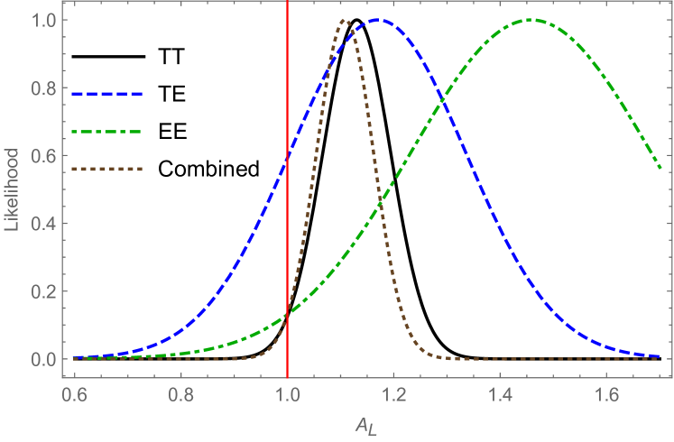
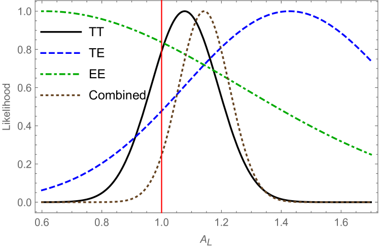
In Figure 6 we plot the likelihoods for , when marginalizing over the rest of parameters, before and after including CIPs.333Note that, since we are using a linear Fisher-matrix analysis, these likelihoods are Gaussian by construction. This Figure shows a significant widening of the likelihood curves, which added to the bias from Eq. (16) is responsible for the decrease in the tension of the fit.
In Table 2 we also show the standard deviations (and new best-fit values) when including the six CDM parameters + (so ). In that case the tension in the TT data set vanishes, due to the correlations between and .
A analysis of the TT power spectrum shows a preference for a non-standard lensing amplitude. The change in from the standard CDM model (with ) to an -varying model (usually denoted CDM+) is , giving rise to a -value of 0.043, which makes it a significantly better fit.
Adding CIPs to this CDM+ model changes by , with a -value of 0.58. This implies that CDM+CIPs does not fit the TT power spectrum better than CDM+.
Interestingly, CIPs alone can do as well as alone improving the statistic. The change in from the CDM model to CDM+CIPs is , with a -value of 0.048 (to be compared with 0.043 when adding a varying to CDM). Notice, though, that the best-fit CIP variance in that case would be , which is in tension with both the trispectrum bound 1306.4319 , and the galaxy-cluster bound 0907.3919 .
This shows that adding either a varying or CIPs to a standard CDM model provides a better fit for the TT Planck power spectrum, by a comparable amount. Adding both, however, is not supported by the data. There are, however, a few systematic effects in the analysis that could bias the result. The most important example is that our treatment of the low- data is too simplistic. As a result, the uncertainties in and in Table 2 are small when compared to the Planck 2015 result 1502.01589 . This indicates that our Fisher-matrix analysis is too optimistic when inferring the optical depth from the low- polarization data, which could be due to the non-gaussian nature of the low- likelihoods, to the mode coupling, or to the linear approximation breaking down. A full likelihood analysis could show that CIPs absorb more of the lensing tension than indicated in this simple analysis.
Summarizing, we conclude that CIPs are unlikely to solve the lensing tension with current Planck data. Nonetheless, they remain one of the simplest prospective solutions, due to their high correlation with the lensing amplitude (). High-quality low- polarization data will be publicly available in the next few years 1407.2584 ; 1408.4789 , so a reanalysis using the full Planck likelihoods, perhaps also including higher- multipoles from SPTpol Austermann:2012ga ; Crites:2014prc , will resolve the matter definitively.
| Parameter | TT | TE | EE | Combined |
|---|---|---|---|---|
| 0.022350.00020 | 0.022570.00032 | 0.02450.0013 | 0.022280.00014 | |
| 0.11800.0023 | 0.1168 0.0023 | 0.10950.0053 | 0.11850.0014 | |
| 0.96600.0054 | 0.9830.015 | 0.9920.014 | 0.96410.0037 | |
| 3.0380.031 | 3.065 0.035 | 3.070.034 | 3.0380.031 | |
| 0.0560.016 | 0.0620.016 | 0.0620.016 | 0.0550.015 | |
| 68.11.0 | 68.61.1 | 72.42.9 | 67.750.64 | |
| 1.130.064 | 1.170.17 | 1.460.23 | 1.1080.054 | |
| Parameter | TT | TE | EE | Combined |
| 0.022480.00029 | 0.02230.0046 | 0.025930.00017 | 0.022220.00018 | |
| 0.11760.0025 | 0.11830.0029 | 0.1102 0.0053 | 0.11870.0015 | |
| 0.96990.0086 | 0.9770.017 | 1.0040.016 | 0.96220.0052 | |
| 3.0410.031 | 3.050.035 | 3.081 0.036 | 3.0370.031 | |
| 0.0570.016 | 0.0580.016 | 0.0650.016 | 0.0540.015 | |
| 68.51.2 | 67.71.5 | 73.03.0 | 67.600.70 | |
| 1.070.11 | 1.430.35 | 0.65 | 1.1420.085 | |
| 0.0070.011 | 0.0280.033 | 0.0880.064 | 0.00380.0074 |
IV.2 Cosmic-variance limit
We now find the minimum observable in the cosmic-variance limited case for different data sets.
We consider an experiment with no instrumental noise (i.e. ), full sky coverage () and range of observation from to 2500. In reality the lowest multipoles should be treated with care, due to possible Galactic-foreground subtraction 1507.02704 , which we ignore here. We show the results for the uncertainties of such an experiment in Table 3.
The best CVL constraints to arise from the polarization power spectra (EE especially) instead of the TT power spectrum, as holds true for the six original parameters 1403.5271 .
The minimum CIP variance observable in the CVL is , a factor of 5 better than the current trispectrum constraint 1306.4319 . This result pales in comparison to the sensitivity of a CVL trispectrum experiment, as described in Ref. 1505.00639 , which would be able to measure .
| Data | |||||||
|---|---|---|---|---|---|---|---|
| TT | 1.6 | 1.7 | 5.0 | 8.1 | 0.019 | 0.80 | 4.8 |
| TE | 1.1 | 1.0 | 4.7 | 3.6 | 8.3 | 0.45 | 2.5 |
| EE | 7.4 | 7.6 | 2.8 | 9.9 | 2.4 | 0.33 | 1.5 |
| Combined | 2.8 | 4.6 | 1.8 | 8.0 | 1.9 | 0.19 | 9.0 |
Here is free, unlike the Planck case, where we included a prior. This leads to higher correlations of the CIP amplitude with the optical depth , and the scalar amplitude . We find the correlation coefficients in the CVL case to be , , , , , and . When including a lensing amplitude, we find .
V Conclusions
Compensated isocurvature perturbations leave no imprint on the observable CMB to linear order, so their amplitude can be considerably larger than the amplitude of primordial adiabatic perturbations. Currently the best constraints arise from analyzing the four-point function of the CMB, from where one can probe the first 20 multipoles of a CIP power spectrum, corresponding to scales larger than 10 degrees in the sky.
We use a different method to search for CIPs, based on studying the CMB power spectrum that arises to second order in the CIP-perturbation amplitude. We find a simple form for the contribution to the CMB power spectrum, proportional to the CIP variance , which has the advantage of being easier to analyze than the trispectrum.
The amplitude of this new contribution to the power spectrum can be expressed in terms of a sum over all the modes of a scale-invariant CIP power spectrum, although only the first modes are important in CMB studies. This allows us to probe the CIPs down to angular scales of 2 degrees in the sky.
We show that CIPs can alleviate the 2 discrepancy in the lensing amplitude , between that inferred from the Planck TT power spectrum and the CDM expectation (). Adding CIPs to a standard CDM model can improve the fit of the TT power spectrum as much as adding a varying , making it unnecessary to have . The best-fit value for in that case, however, would be three standard deviations above the current bounds. A full MCMC analysis would precisely determine whether CIPs provide a viable solution to the lensing tension.
We find a 1 constraint on the CIP variance of using Planck temperature data alone, which improves to if polarization data are included. This result is of the same order of magnitude as the current trispectrum bound, but this analysis is far simpler and more intuitive, as well as less computationally costly. We also forecast the minimum CIP amplitude observable with a cosmic-variance-limited measurement of the CMB power spectra to be . This result is a factor of better than the current constraints, promising ever more precise constraints of the uniformity of the primordial baryon fraction.
Acknowledgements.
We thank David Spergel, Tristan Smith, Graeme Addison, Marius Millea, Wayne Hu, and Silvia Galli for very useful and instructive discussions, as well as the anonymous referee for helpful comments. JBM, LD, MK, and EDK are funded at Johns Hopkins University by the John Templeton Foundation, the Simons Foundation, NSF grant PHY-1214000, and NASA ATP grant NNX15AB18G. DG is funded at the University of Chicago by a National Science Foundation Astronomy and Astrophysics Postdoctoral Fellowship under Award NO. AST-1302856. This work was supported in part by the Kavli Institute for Cosmological Physics at the University of Chicago through grant NSF PHY-1125897 and an endowment from the Kavli Foundation and its founder Fred Kavli. LD is also supported at the Institute for Advanced Study by NASA through Einstein Postdoctoral Fellowship grant number PF5-160135 awarded by the Chandra X-ray Center, which is operated by the Smithsonian Astrophysical Observatory for NASA under contract NAS8-03060.References
- (1) V. F. Mukhanov, JETP Lett. 41, 493 (1985) [Pisma Zh. Eksp. Teor. Fiz. 41, 402 (1985)].
- (2) V. Springel et al., Nature 435, 629 (2005), astro-ph/0504097.
- (3) J. M. Bardeen, P. J. Steinhardt and M. S. Turner, Phys. Rev. D 28, 679 (1983).
- (4) C. P. Ma and E. Bertschinger, Astrophys. J. 455, 7 (1995), astro-ph/9506072.
- (5) P. A. R. Ade et al. [Planck Collaboration], arXiv:1502.01589.
- (6) P. J. E. Peebles and J. T. Yu, Astrophys. J. 162, 815 (1970).
- (7) A. D. Linde and V. F. Mukhanov, Phys. Rev. D 56, 535 (1997), astro-ph/9610219.
- (8) C. Gordon, D. Wands, B. A. Bassett and R. Maartens, Phys. Rev. D 63, 023506 (2001), astro-ph/0009131.
- (9) W. Hu, Phys. Rev. D 59, 021301 (1999), astro-ph/9809142.
- (10) D. H. Lyth and D. Wands, Phys. Lett. B 524, 5 (2002), hep-ph/0110002.
- (11) D. H. Lyth, C. Ungarelli and D. Wands, Phys. Rev. D 67, 023503 (2003), astro-ph/0208055.
- (12) M. Beltran, J. Garcia-Bellido, J. Lesgourgues and A. Riazuelo, Phys. Rev. D 70, 103530 (2004), astro-ph/0409326.
- (13) M. Beltran, J. Garcia-Bellido, J. Lesgourgues and M. Viel, Phys. Rev. D 72, 103515 (2005), astro-ph/0509209.
- (14) M. Kawasaki and T. Sekiguchi, Prog. Theor. Phys. 120, 995 (2008), arXiv:0705.2853.
- (15) C. Gordon and A. Lewis, Phys. Rev. D 67, 123513 (2003), astro-ph/0212248.
- (16) C. Gordon and J. R. Pritchard, Phys. Rev. D 80, 063535 (2009), arXiv:0907.5400.
- (17) G. P. Holder, K. M. Nollett and A. van Engelen, Astrophys. J. 716, 907 (2010), arXiv:0907.3919.
- (18) D. Grin, O. Doré and M. Kamionkowski, Phys. Rev. D 84, 123003 (2011), arXiv:1107.5047.
- (19) D. Grin, O. Doré and M. Kamionkowski, Phys. Rev. Lett. 107, 261301 (2011), arXiv:1107.1716.
- (20) D. Grin, D. Hanson, G. P. Holder, O. Doré and M. Kamionkowski, Phys. Rev. D 89, 023006 (2014), arXiv:1306.4319.
- (21) C. He, D. Grin and W. Hu, Phys. Rev. D 92, no. 6, 063018 (2015), arXiv:1505.00639.
- (22) G. Hinshaw et al. [WMAP Collaboration], Astrophys. J. Suppl. 208, 19 (2013), arXiv:1212.5226.
- (23) A. Lewis and S. Bridle, Phys. Rev. D 66, 103511 (2002), astro-ph/0205436.
- (24) B. Audren, J. Lesgourgues, K. Benabed and S. Prunet, JCAP 1302, 001 (2013), arXiv:1210.7183.
- (25) A. Lewis, A. Challinor and A. Lasenby, Astrophys. J. 538, 473 (2000), astro-ph/9911177.
- (26) G. Jungman, M. Kamionkowski, A. Kosowsky and D. N. Spergel, Phys. Rev. D 54, 1332 (1996) astro-ph/9512139.
- (27) M. Tegmark, A. Taylor and A. Heavens, Astrophys. J. 480, 22 (1997), astro-ph/9603021.
- (28) S. Galli et al., Phys. Rev. D 90, 063504 (2014), arXiv:1403.5271.
- (29) M. Kamionkowski, A. Kosowsky and A. Stebbins, Phys. Rev. D 55, 7368 (1997), astro-ph/9611125.
- (30) M. Zaldarriaga and U. Seljak, Phys. Rev. D 55, 1830 (1997), astro-ph/9609170.
- (31) J. R. Bond and G. Efstathiou, Mon. Not. Roy. Astron. Soc. 226, 655 (1987).
- (32) K. L. Ng and K. W. Ng, Astrophys. J. 456, 413 (1996) astro-ph/9412097.
- (33) M. Zaldarriaga, Phys. Rev. D 55, 1822 (1997), astro-ph/9608050.
- (34) G. Holder, Z. Haiman, M. Kaplinghat and L. Knox, Astrophys. J. 595, 13 (2003), astro-ph/0302404.
- (35) A. Lewis and A. Challinor, Phys. Rept. 429, 1 (2006), astro-ph/0601594.
- (36) P. A. R. Ade et al. [Planck Collaboration], arXiv:1502.01591.
- (37) E. Calabrese, A. Slosar, A. Melchiorri, G. F. Smoot and O. Zahn, Phys. Rev. D 77, 123531 (2008), arXiv:0803.2309.
- (38) M. Zaldarriaga and U. Seljak, Phys. Rev. D 58, 023003 (1998), astro-ph/9803150.
- (39) E. Di Valentino, A. Melchiorri and J. Silk, arXiv:1507.06646.
- (40) E. Di Valentino, A. Melchiorri and J. Silk, arXiv:1509.07501.
- (41) J. Lazear et al., Proc. SPIE Int. Soc. Opt. Eng. 9153, 91531L (2014), arXiv:1407.2584.
- (42) J. W. Appel et al., Proc. SPIE Int. Soc. Opt. Eng. 9153, 91531J (2014), arXiv:1408.4789.
- (43) J. E. Austermann et al., Proc. SPIE Int. Soc. Opt. Eng. 8452, 84521E (2012) doi:10.1117/12.927286 arXiv:1210.4970.
- (44) A. T. Crites et al. [SPT Collaboration], Astrophys. J. 805, no. 1, 36 (2015) doi:10.1088/0004-637X/805/1/36 arXiv:1411.1042.
- (45) N. Aghanim et al. [Planck Collaboration], arXiv:1507.02704.