Fisher Matrix Optimization of Cosmic Microwave Background Interferometers

Haonan Liu haonan.liu@richmond.edu โ€ƒโ€ƒ Emory F. Bunn Physics Department, University of Richmond, Richmond, VA 23173
Abstract

We describe a method for forecasting errors in interferometric measurements of polarization of the cosmic microwave background (CMB) radiation, based on the use of the Fisher matrix calculated from the visibility covariance and relation matrices. In addition to noise and sample variance, the method can account for many kinds of systematic error by calculating an augmented Fisher matrix, including parameters that characterize the instrument along with the cosmological parameters to be estimated. The method is illustrated with examples of gain errors and errors in polarizer orientation. The augmented Fisher matrix approach is applicable to a much wider range of problems beyond CMB interferometry.

I Introduction

Observations of the cosmic microwave background (CMB) are among the chief drivers of the revolutionary advances in cosmology over the past 20 years (see, e.g., Hu (2003); Challinor (2013) and references therein), and further observations, particularly of CMB polarization, are likely to be of major importance in the coming years. CMB polarization can probe the early Universe in a wide variety of ways, including possibly providing direct evidence of a stochastic gravitational wave background, which would give direct evidence in support of inflation Zaldarriaga and Seljak (1997); Seljak and Zaldarriaga (1997); Kamionkowski etย al. (1997a, b).

The key to analyzing CMB polarization data is the separation of the signal into a scalar E๐ธE component and a pseudoscalar B๐ตB component. The inflationary signal is sought in the B๐ตB component. Because this component is predicted to be significantly weaker than the E๐ธE component (and both are much weaker than the temperature anisotropy), detection of B๐ตB modes is a daunting task.

Control of systematic errors will be vital to the success of the quest to characterize B modes. In particular, some errors may cause โ€œleakageโ€ into the B๐ตB signal from the much larger E๐ธE and temperature anisotropy (T๐‘‡T) signals. (Such leakage occurs even in the absence of systematic errors. See, e.g., Lewis etย al. (2002); Bunn (2002a, b); Bunn etย al. (2003); Bunn (2011); Kim (2011); Bowyer etย al. (2011); Lewis (2003); Park and Ng (2004); Smith (2006a, b); Smith and Zaldarriaga (2007); Cao and Fang (2009); Zhao and Baskaran (2010).) In considering the design of future instruments, methods of assessing the severity of various sources of error are quite valuable. Detailed simulations (e.g., Karakci etย al. (2013a); Zhang etย al. (2013); Karakci etย al. (2013b); Sutter etย al. (2012)) often provide the best assessment, but approximate analytic methods (e.g., Hu etย al. (2003); Bunn (2007)) can provide valuable insight before undertaking the computational effort of a full simulation.

In this paper, we describe a Fisher-matrix method for assessing the ability of interferometric instruments to detect CMB polarization signals, with particular emphasis on the effect of systematic errors. Interferometers have been important in CMB science in the past, including making some of the early detections of CMB polarization Readhead etย al. (2004); Leitch etย al. (2005). The formalism for analyzing interferometric CMB observations has been well-developed Hobson etย al. (1995); Hobson and Magueijo (1996); White etย al. (1999); Hobson and Maisinger (2002); Myers etย al. (2003); Bunn and White (2006) Although most current and planned instruments are traditional imaging telescopes, at least one interferometer is under development Piat etย al. (2012); Ghribi etย al. (2014). Interferometers and imaging telescopes have quite different susceptibility to various sources of error, so it would seem worthwhile to develop tools to understand both approaches.

The method described in this paper uses Fisher matrices to forecast the errors on cosmological parameters obtainable from a given instrument. After developing the general method for calculating Fisher matrices and the resulting error forecasts for an ideal (systematic-error-free) interferometer, we extend the method to allow consideration of systematic effects. In particular, we calculate an โ€œaugmented Fisher matrix,โ€ in which we treat parameters describing the various systematic effects as unknowns to be estimated along with the cosmological parameters of interest. The resulting Fisher matrices allow us to forecast the errors expected on cosmological parameters, taking into account our ignorance of the systematic error parameters.

Although we apply our formalism to the specific case of CMB polarization measurements, the approach we describe has broader applicability. In particular, upcoming efforts to map the Universe through 21-cm tomography (see, e.g., Pritchard and Loeb (2012); Morales and Wyithe (2010) and references therein) involve the extraction of faint signals from interferometric data sets and hence have significant overlap with CMB polarization. It would be of interest to explore the generalization of our approach to this class of observations.

The remainder of this paper is organized as follows. Section II lays out the formalism for calculating covariance matrices and Fisher matrices for interferometers, including systematic effects. Section III reviews the approximate analytic treatment of systematic effects in ref.ย Bunn (2007). Section IV presents the results of a variety of tests of the method, and Section V provides a brief discussion.
Refer to caption
Refer to caption
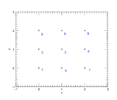
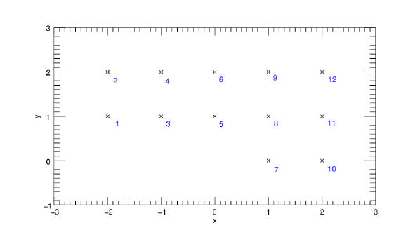
Figure 1: A close-packed square array and its corresponding baseline graph with Na=3subscript๐‘๐‘Ž3N_{a}=3.

II Formalism

II.1 Visibilities

Consider a close-packed square array with Nasubscript๐‘๐‘ŽN_{a} antennas on each side. For antennas j๐‘—j and k๐‘˜k that are separated by the vector ฮดโ€‹๐ซ=(x,y)๐›ฟ๐ซ๐‘ฅ๐‘ฆ\delta\mathbf{r}=(x,y) on the antenna map, the baseline ๐ฎ๐ฎ\mathbf{u} has the form

๐ฎ=ฮดโ€‹๐ซโ€‹ฮ”โ€‹u=(xโ€‹ฮ”โ€‹u,yโ€‹ฮ”โ€‹u).๐ฎ๐›ฟ๐ซฮ”๐‘ข๐‘ฅฮ”๐‘ข๐‘ฆฮ”๐‘ข\mathbf{u}=\delta\mathbf{r}\Delta u=(x\Delta u,y\Delta u). (1)

Here x๐‘ฅx and y๐‘ฆy are any integers that satisfy โˆ’(Naโˆ’1)โฉฝx,yโฉฝNaโˆ’1formulae-sequencesubscript๐‘๐‘Ž1๐‘ฅ๐‘ฆsubscript๐‘๐‘Ž1-(N_{a}-1)\leqslant x,y\leqslant N_{a}-1. The baseline for two adjacent antennas is ฮ”โ€‹u=D/ฮปฮ”๐‘ข๐ท๐œ†\Delta u=D/\lambda, where D๐ทD is the antenna diameter. We will assume diffraction-limited antennas, for which the Gaussian beam width is b=0.518โ€‹ฮป/D๐‘0.518๐œ†๐ทb=0.518\lambda/D, so that ฮ”โ€‹u=0.518/bฮ”๐‘ข0.518๐‘\Delta u=0.518/b.

The total number of independent baselines is 12โ€‹[(2โ€‹Naโˆ’1)2โˆ’1]12delimited-[]superscript2subscript๐‘๐‘Ž121\frac{1}{2}[(2N_{a}-1)^{2}-1], where the โˆ’11-1 appears because we do not include the case x=y=0๐‘ฅ๐‘ฆ0x=y=0, and the 1212\frac{1}{2} is included to avoid redundancy since Vโ€‹(๐ฎ)=Vโˆ—โ€‹(โˆ’๐ฎ)๐‘‰๐ฎsuperscript๐‘‰๐ฎV(\mathbf{u})=V^{*}(-\mathbf{u}). We include all baselines with y>0๐‘ฆ0y>0 and all with y=0๐‘ฆ0y=0 and xโ‰ฅ0๐‘ฅ0x\geq 0, labeling them in the order shown in Figure 1.

Now, suppose a monochromatic plane wave with angular frequency ฯ‰=2โ€‹ฯ€โ€‹c/ฮป๐œ”2๐œ‹๐‘๐œ†\omega=2\pi c/\lambda that approaches the center of one antenna from the direction ๐ซ^^๐ซ\hat{\mathbf{r}} has the form

๐„=ฯตโ€‹(๐ซ^)โ€‹eiโ€‹(ฯ‰โ€‹tโˆ’๐คโ‹…๐ฑ),๐„bold-italic-ฯต^๐ซsuperscript๐‘’๐‘–๐œ”๐‘กโ‹…๐ค๐ฑ\mathbf{E}=\boldsymbol{\epsilon}(\hat{\mathbf{r}})e^{i(\omega t-\mathbf{k}\cdot\mathbf{x})}, (2)

where ๐ค๐ค\mathbf{k} is the wavevector defined by ๐ค=โˆ’(2โ€‹ฯ€/ฮป)โ€‹r^๐ค2๐œ‹๐œ†^๐‘Ÿ\mathbf{k}=-(2\pi/\lambda)\hat{r}. Then the 2ร—2222\times 2 matrix of visibilities corresponding to a given baseline ๐ฎ๐ฎ\mathbf{u} is Bunn (2007)

๐•โ€‹(๐ฎ)=โˆซ๐’โ€‹(๐ซ)โ€‹Aโ€‹(๐ซ)โ€‹e2โ€‹ฯ€โ€‹iโ€‹๐ฎโ‹…๐ซโ€‹d2โ€‹๐ซ,๐•๐ฎ๐’๐ซ๐ด๐ซsuperscript๐‘’โ‹…2๐œ‹๐‘–๐ฎ๐ซsuperscript๐‘‘2๐ซ\mathbf{V}(\mathbf{u})=\int{\mathbf{S}(\mathbf{r})A(\mathbf{r})e^{2\pi i\mathbf{u}\cdot\mathbf{r}}d^{2}\mathbf{r}}, (3)

where the Stokes matrix ๐’๐’\mathbf{S} is given by

๐’=(SXโ€‹XSXโ€‹YSYโ€‹XSYโ€‹Y)=(I+QU+iโ€‹VUโˆ’iโ€‹VIโˆ’Q),๐’matrixsubscript๐‘†๐‘‹๐‘‹subscript๐‘†๐‘‹๐‘Œsubscript๐‘†๐‘Œ๐‘‹subscript๐‘†๐‘Œ๐‘Œmatrix๐ผ๐‘„๐‘ˆ๐‘–๐‘‰๐‘ˆ๐‘–๐‘‰๐ผ๐‘„\begin{split}{\bf S}&=\begin{pmatrix}S_{XX}&S_{XY}\\ S_{YX}&S_{YY}\end{pmatrix}\\ &=\begin{pmatrix}I+Q&U+iV\\ U-iV&I-Q\end{pmatrix},\end{split} (4)

and Aโ€‹(๐ซ)๐ด๐ซA(\mathbf{r}) is the antenna pattern, which we will take to be Gaussian,

Aโ€‹(๐ซ)=eโˆ’๐ซ2/2โ€‹b2๐ด๐ซsuperscript๐‘’superscript๐ซ22superscript๐‘2A(\mathbf{r})=e^{-\mathbf{r}^{2}/{2b^{2}}} (5)

with b๐‘b the beam size. Note that we are considering experiments that combine linear polarization states (X,Y)๐‘‹๐‘Œ(X,Y), not circular polarization states.

We define Stokes Q๐‘„Q and U๐‘ˆU visibilities,

VQโ‰กVQโ€‹(๐ฎ)=โˆซQโ€‹(๐ซ)โ€‹Aโ€‹(๐ซ)โ€‹e2โ€‹ฯ€โ€‹iโ€‹๐ฎโ‹…๐ซโ€‹d2โ€‹๐ซ,subscript๐‘‰๐‘„subscript๐‘‰๐‘„๐ฎ๐‘„๐ซ๐ด๐ซsuperscript๐‘’โ‹…2๐œ‹๐‘–๐ฎ๐ซsuperscript๐‘‘2๐ซ\displaystyle V_{Q}\equiv V_{Q}(\mathbf{u})=\int{Q(\mathbf{r})A(\mathbf{r})e^{2\pi i\mathbf{u}\cdot\mathbf{r}}d^{2}\mathbf{r}}, (6)
VUโ‰กVUโ€‹(๐ฎ)=โˆซUโ€‹(๐ซ)โ€‹Aโ€‹(๐ซ)โ€‹e2โ€‹ฯ€โ€‹iโ€‹๐ฎโ‹…๐ซโ€‹d2โ€‹๐ซ.subscript๐‘‰๐‘ˆsubscript๐‘‰๐‘ˆ๐ฎ๐‘ˆ๐ซ๐ด๐ซsuperscript๐‘’โ‹…2๐œ‹๐‘–๐ฎ๐ซsuperscript๐‘‘2๐ซ\displaystyle V_{U}\equiv V_{U}(\mathbf{u})=\int{U(\mathbf{r})A(\mathbf{r})e^{2\pi i\mathbf{u}\cdot\mathbf{r}}d^{2}\mathbf{r}}. (7)

As usual in CMB studies, we will express Stokes parameters and their associated visibilities in thermodynamic temperature units.

By the convolution theorem,

VQ=(2โ€‹ฯ€)2โ€‹โˆซโˆซQ~โ€‹(๐ค)โ€‹A~โˆ—โ€‹(๐ค+2โ€‹ฯ€โ€‹๐ฎ)โ€‹d2โ€‹๐ค,subscript๐‘‰๐‘„superscript2๐œ‹2~๐‘„๐คsuperscript~๐ด๐ค2๐œ‹๐ฎsuperscript๐‘‘2๐ค\displaystyle V_{Q}=(2\pi)^{2}\int{\int{\tilde{Q}(\mathbf{k})\tilde{A}^{*}(\mathbf{k}+2\pi\mathbf{u})d^{2}\mathbf{k}}}, (8)
VU=(2โ€‹ฯ€)2โ€‹โˆซโˆซU~โ€‹(๐ค)โ€‹A~โˆ—โ€‹(๐ค+2โ€‹ฯ€โ€‹๐ฎ)โ€‹d2โ€‹๐ค,subscript๐‘‰๐‘ˆsuperscript2๐œ‹2~๐‘ˆ๐คsuperscript~๐ด๐ค2๐œ‹๐ฎsuperscript๐‘‘2๐ค\displaystyle V_{U}=(2\pi)^{2}\int{\int{\tilde{U}(\mathbf{k})\tilde{A}^{*}(\mathbf{k}+2\pi\mathbf{u})d^{2}\mathbf{k}}}, (9)

where the tilde denotes a two-dimensional Fourier transform in the flat-sky approximation.

From equation (4), we can see that the Q๐‘„Q and U๐‘ˆU visibilities are related to the visibility matrix ๐•๐•\mathbf{V} by

VQ=12โ€‹(VXโ€‹Xโˆ’VYโ€‹Y),subscript๐‘‰๐‘„12subscript๐‘‰๐‘‹๐‘‹subscript๐‘‰๐‘Œ๐‘Œ\displaystyle V_{Q}=\frac{1}{2}(V_{XX}-V_{YY}), (10)
VU=12โ€‹(VXโ€‹Y+VYโ€‹X).subscript๐‘‰๐‘ˆ12subscript๐‘‰๐‘‹๐‘Œsubscript๐‘‰๐‘Œ๐‘‹\displaystyle V_{U}=\frac{1}{2}(V_{XY}+V_{YX}). (11)

In practice, we do not usually use (10) to measure VQsubscript๐‘‰๐‘„V_{Q}, as it involves cancellation of the large contribution from Stokes I๐ผI. Instead, we usually measure VQsubscript๐‘‰๐‘„V_{Q} by rotating the axes for our polarization basis through 45ยฐย and then using equation (11).

The Stokes parameters are related to the E and B modes in the following way:

Q~โ€‹(๐ค)~๐‘„๐ค\displaystyle\tilde{Q}(\mathbf{k}) =E~โ€‹(๐ค)โ€‹cosโก(2โ€‹ฯ•)+B~โ€‹(๐ค)โ€‹sinโก(2โ€‹ฯ•),absent~๐ธ๐ค2italic-ฯ•~๐ต๐ค2italic-ฯ•\displaystyle=\tilde{E}(\mathbf{k})\cos(2\phi)+\tilde{B}(\mathbf{k})\sin(2\phi), (12)
U~โ€‹(๐ค)~๐‘ˆ๐ค\displaystyle\tilde{U}(\mathbf{k}) =โˆ’E~โ€‹(๐ค)โ€‹sinโก(2โ€‹ฯ•)+B~โ€‹(๐ค)โ€‹cosโก(2โ€‹ฯ•),absent~๐ธ๐ค2italic-ฯ•~๐ต๐ค2italic-ฯ•\displaystyle=-\tilde{E}(\mathbf{k})\sin(2\phi)+\tilde{B}(\mathbf{k})\cos(2\phi), (13)

where ฯ•italic-ฯ•\phi is the angle between the vector ๐ค๐ค\mathbf{k} and the x๐‘ฅx axis. We assume that the E๐ธE and B๐ตB contributions are independent, statistically isotropic random fields with the flat-sky power spectra PE,PBsubscript๐‘ƒ๐ธsubscript๐‘ƒ๐ตP_{E},P_{B}, which are defined as PE,Bโ€‹(k)=ClE,Bsubscript๐‘ƒ๐ธ๐ต๐‘˜superscriptsubscript๐ถ๐‘™๐ธ๐ตP_{E,B}(k)=C_{l}^{E,B} with l=k๐‘™๐‘˜l=k. Then

โŸจE~โ€‹(๐ค1)โ€‹E~โˆ—โ€‹(๐ค2)โŸฉ=PEโ€‹(k1)(2โ€‹ฯ€)2โ€‹ฮดโ€‹(๐ค1โˆ’๐ค2),delimited-โŸจโŸฉ~๐ธsubscript๐ค1superscript~๐ธsubscript๐ค2subscript๐‘ƒ๐ธsubscript๐‘˜1superscript2๐œ‹2๐›ฟsubscript๐ค1subscript๐ค2\langle\tilde{E}({\bf k}_{1})\tilde{E}^{*}({\bf k}_{2})\rangle=\frac{P_{E}(k_{1})}{(2\pi)^{2}}\delta({\bf k}_{1}-{\bf k}_{2}), (14)

with a similar expression for B. The extra (2โ€‹ฯ€)2superscript2๐œ‹2(2\pi)^{2} factor is caused by the approximation of a flat-sky power spectrum from a full sky power spectrum.

We then have

โŸจQ~โ€‹(๐ค1)โ€‹Q~โˆ—โ€‹(๐ค2)โŸฉdelimited-โŸจโŸฉ~๐‘„subscript๐ค1superscript~๐‘„subscript๐ค2\displaystyle\langle\tilde{Q}(\mathbf{k}_{1})\tilde{Q}^{*}(\mathbf{k}_{2})\rangle =ฮดโ€‹(๐ค1โˆ’๐ค2)/(2โ€‹ฯ€)2absent๐›ฟsubscript๐ค1subscript๐ค2superscript2๐œ‹2\displaystyle=\delta(\mathbf{k}_{1}-\mathbf{k}_{2})/(2\pi)^{2}
[PEโ€‹(๐ค)โ€‹cos2โก(2โ€‹ฯ•)+PBโ€‹(๐ค)โ€‹sin2โก(2โ€‹ฯ•)],delimited-[]subscript๐‘ƒ๐ธ๐คsuperscript22italic-ฯ•subscript๐‘ƒ๐ต๐คsuperscript22italic-ฯ•\displaystyle[P_{E}(\mathbf{k})\cos^{2}(2\phi)+P_{B}(\mathbf{k})\sin^{2}(2\phi)], (15)
โŸจU~โ€‹(๐ค1)โ€‹U~โˆ—โ€‹(๐ค2)โŸฉdelimited-โŸจโŸฉ~๐‘ˆsubscript๐ค1superscript~๐‘ˆsubscript๐ค2\displaystyle\langle\tilde{U}(\mathbf{k}_{1})\tilde{U}^{*}(\mathbf{k}_{2})\rangle =ฮดโ€‹(๐ค1โˆ’๐ค2)/(2โ€‹ฯ€)2absent๐›ฟsubscript๐ค1subscript๐ค2superscript2๐œ‹2\displaystyle=\delta(\mathbf{k}_{1}-\mathbf{k}_{2})/(2\pi)^{2}
[PEโ€‹(๐ค)โ€‹sin2โก(2โ€‹ฯ•)+PBโ€‹(๐ค)โ€‹cos2โก(2โ€‹ฯ•)],delimited-[]subscript๐‘ƒ๐ธ๐คsuperscript22italic-ฯ•subscript๐‘ƒ๐ต๐คsuperscript22italic-ฯ•\displaystyle[P_{E}(\mathbf{k})\sin^{2}(2\phi)+P_{B}(\mathbf{k})\cos^{2}(2\phi)], (16)
โŸจQ~โ€‹(๐ค1)โ€‹U~โˆ—โ€‹(๐ค2)โŸฉdelimited-โŸจโŸฉ~๐‘„subscript๐ค1superscript~๐‘ˆsubscript๐ค2\displaystyle\langle\tilde{Q}(\mathbf{k}_{1})\tilde{U}^{*}(\mathbf{k}_{2})\rangle =ฮดโ€‹(๐ค1โˆ’๐ค2)/(2โ€‹ฯ€)2absent๐›ฟsubscript๐ค1subscript๐ค2superscript2๐œ‹2\displaystyle=\delta(\mathbf{k}_{1}-\mathbf{k}_{2})/(2\pi)^{2}
[โˆ’12โ€‹PEโ€‹(๐ค)โ€‹sinโก(4โ€‹ฯ•)+12โ€‹PBโ€‹(๐ค)โ€‹sin2โก(2โ€‹ฯ•)].delimited-[]12subscript๐‘ƒ๐ธ๐ค4italic-ฯ•12subscript๐‘ƒ๐ต๐คsuperscript22italic-ฯ•\displaystyle[-\frac{1}{2}P_{E}(\mathbf{k})\sin(4\phi)+\frac{1}{2}P_{B}(\mathbf{k})\sin^{2}(2\phi)]. (17)

We will use these results in the next section for the deduction of the visibility covariance matrix.

For regular arrays of the sort considered here, multiple pairs of antennas can have the same separation vector ฮดโ€‹๐ซ๐›ฟ๐ซ\delta{\bf r} and hence correspond to the same baseline. We refer to the visibility measured from a given antenna pair as a โ€œmicro-visibilityโ€ and say that multiple micro-visibilities correspond to the same โ€œmacro-visibility.โ€ Since all micro-visibilities corresponding to a given macro-visibility should be equal (in the absence of noise), we average them together to get the measured value of the macro-visibility.

To be specific, let VJsubscript๐‘‰๐ฝV_{J} represent the J๐ฝJth macro-visibility. Let SJsubscript๐‘†๐ฝS_{J} be the set of all micro-visibilities corresponding to that macro-visibility, with each micro-visibility labeled by a pair of antennas (aโ€‹b)๐‘Ž๐‘(ab). Also let NJsubscript๐‘๐ฝN_{J} be the number of micro-visibilities corresponding to that macro-visibility (i.e., the cardinality of SJsubscript๐‘†๐ฝS_{J}). Then

VXโ€‹J=1NJโ€‹โˆ‘(aโ€‹b)โˆˆSJVX(aโ€‹b),subscript๐‘‰๐‘‹๐ฝ1subscript๐‘๐ฝsubscript๐‘Ž๐‘subscript๐‘†๐ฝsuperscriptsubscript๐‘‰๐‘‹๐‘Ž๐‘V_{XJ}={1\over N_{J}}\sum_{(ab)\in S_{J}}V_{X}^{(ab)}, (18)

where Xโˆˆ{Q,U}๐‘‹๐‘„๐‘ˆX\in\{Q,U\}, and VX(aโ€‹b)superscriptsubscript๐‘‰๐‘‹๐‘Ž๐‘V_{X}^{(ab)} labels a micro-visibility.

For instance, consider a 3ร—3333\times 3 array with antennas labeled from 1 to 9 as in Figure 1. There are twelve macro-visibilities. Using the numbering scheme in the figure, J=7๐ฝ7J=7 corresponds to the macro-visibility (1,0)10(1,0) โ€“ that is, to antennas that are separated by one unit in the x๐‘ฅx direction and zero units in the y๐‘ฆy direction. Then

S7={(14),(25),(36),(47),(58),(69)},subscript๐‘†7142536475869S_{7}=\{(14),(25),(36),(47),(58),(69)\}, (19)

and of course N7=6subscript๐‘76N_{7}=6.

II.2 Fisher Information Matrix

II.2.1 Real Values

Although we will be working with complex data (visibilities), we begin by reviewing the Fisher matrix formalism for real data.

Let rโ†’=(r1,โ€ฆ,rn)Tโ†’๐‘Ÿsuperscriptsubscript๐‘Ÿ1โ€ฆsubscript๐‘Ÿ๐‘›๐‘‡\vec{r}=(r_{1},\ldots,r_{n})^{T} be a random vector drawn from a multivariate normal distribution with mean zero and covariance matrix ๐šช๐šช{\boldsymbol{\Gamma}} with elements

ฮ“jโ€‹k=โŸจriโ€‹rjโŸฉ.subscriptฮ“๐‘—๐‘˜delimited-โŸจโŸฉsubscript๐‘Ÿ๐‘–subscript๐‘Ÿ๐‘—\Gamma_{jk}=\langle r_{i}r_{j}\rangle. (20)

The probability density for rโ†’โ†’๐‘Ÿ\vec{r} is

fโ€‹(rโ†’)=eโˆ’12โ€‹rโ†’Tโ€‹๐šชโˆ’1โ€‹rโ†’(2โ€‹ฯ€)n/2โ€‹det1/2(๐šช).๐‘“โ†’๐‘Ÿsuperscript๐‘’12superscriptโ†’๐‘Ÿ๐‘‡superscript๐šช1โ†’๐‘Ÿsuperscript2๐œ‹๐‘›2superscript12๐šชf(\vec{r})={e^{-{1\over 2}\vec{r}^{T}{\boldsymbol{\Gamma}}^{-1}\vec{r}}\over(2\pi)^{n/2}\det^{1/2}({\boldsymbol{\Gamma}})}. (21)

Now suppose that ๐šช๐šช{\boldsymbol{\Gamma}} is a function of some set of m๐‘šm parameters ฮธ1,ฮธ2,โ€ฆ,ฮธmsubscript๐œƒ1subscript๐œƒ2โ€ฆsubscript๐œƒ๐‘š\theta_{1},\theta_{2},\ldots,\theta_{m}. These may be cosmological parameters which we would like to estimate from the data, but as we will see they can also be parameters characterizing the experiment itself (e.g., the gain on an antenna or the orientation of a polarizer).

We define the likelihood function

Lโ€‹(ฮธโ†’)=fโ€‹(rโ†’|ฮธโ†’).๐ฟโ†’๐œƒ๐‘“conditionalโ†’๐‘Ÿโ†’๐œƒL(\vec{\theta})=f(\vec{r}|\vec{\theta}). (22)

For convenience, define the log-likelihood function

โ„’=โˆ’lnโกL=12โ€‹rโ†’Tโ€‹๐šชโˆ’1โ€‹rโ†’+12โ€‹lnโ€‹det(๐šช)+n2โ€‹lnโก(2โ€‹ฯ€).โ„’๐ฟ12superscriptโ†’๐‘Ÿ๐‘‡superscript๐šช1โ†’๐‘Ÿ12๐šช๐‘›22๐œ‹{\cal L}=-\ln L={1\over 2}\vec{r}^{T}{\boldsymbol{\Gamma}}^{-1}\vec{r}+{1\over 2}\ln\det({\boldsymbol{\Gamma}})+{n\over 2}\ln(2\pi). (23)

Then the Fisher Information Matrix is defined to have elements

Fjโ€‹k=โŸจโˆ‚2โ„’โˆ‚ฮธjโ€‹โˆ‚ฮธkโŸฉ,subscript๐น๐‘—๐‘˜delimited-โŸจโŸฉsuperscript2โ„’subscript๐œƒ๐‘—subscript๐œƒ๐‘˜F_{jk}=\left<{\partial^{2}{\cal L}\over\partial\theta_{j}\partial\theta_{k}}\right>, (24)

which can be shown to be

Fjโ€‹k=12โ€‹Trโ€‹(๐šชโˆ’1โ€‹dโ€‹๐šชdโ€‹ฮธjโ€‹๐šชโˆ’1โ€‹dโ€‹๐šชdโ€‹ฮธk).subscript๐น๐‘—๐‘˜12Trsuperscript๐šช1๐‘‘๐šช๐‘‘subscript๐œƒ๐‘—superscript๐šช1๐‘‘๐šช๐‘‘subscript๐œƒ๐‘˜F_{jk}={1\over 2}{\rm Tr}\left({\boldsymbol{\Gamma}}^{-1}{d{\boldsymbol{\Gamma}}\over d\theta_{j}}{\boldsymbol{\Gamma}}^{-1}{d{\boldsymbol{\Gamma}}\over d\theta_{k}}\right). (25)

The Fisher matrix tells us the expected errors on the parameters. In particular, 1/Fiโ€‹i1subscript๐น๐‘–๐‘–1/\sqrt{F_{ii}} is the expected error on ฮธisubscript๐œƒ๐‘–\theta_{i} assuming all the other parameters are known, and (Fโˆ’1)iโ€‹isubscriptsuperscript๐น1๐‘–๐‘–\sqrt{(F^{-1})_{ii}} is the optimal error on ฮธisubscript๐œƒ๐‘–\theta_{i} assuming all other parameters are unknown (e.g, Berger (1993)).

II.2.2 Complex Values

We now consider complex vectors. Let zโ†’=(z1,โ€ฆ,zn)Tโ†’๐‘งsuperscriptsubscript๐‘ง1โ€ฆsubscript๐‘ง๐‘›๐‘‡\vec{z}=(z_{1},\ldots,z_{n})^{T} be a vector of complex Gaussian random numbers with zero mean (e.g., a set of visibilities). One way to proceed is to think of this n๐‘›n-dimensional complex vector as a 2โ€‹n2๐‘›2n-dimensional real vector. To be specific, let xโ†’=Reโ€‹(zโ†’)โ†’๐‘ฅReโ†’๐‘ง\vec{x}={\rm Re}(\vec{z}) and yโ†’=Imโ€‹(zโ†’)โ†’๐‘ฆImโ†’๐‘ง\vec{y}={\rm Im}(\vec{z}), and define

rโ†’=(xโ†’yโ†’)=(x1โ‹ฎxny1โ‹ฎyn).โ†’๐‘Ÿmatrixโ†’๐‘ฅโ†’๐‘ฆmatrixsubscript๐‘ฅ1โ‹ฎsubscript๐‘ฅ๐‘›subscript๐‘ฆ1โ‹ฎsubscript๐‘ฆ๐‘›\vec{r}=\begin{pmatrix}\vec{x}\\ \vec{y}\end{pmatrix}=\begin{pmatrix}x_{1}\\ \vdots\\ x_{n}\\ y_{1}\\ \vdots\\ y_{n}\end{pmatrix}. (26)

Then define a 2โ€‹nร—2โ€‹n2๐‘›2๐‘›2n\times 2n covariance matrix

๐šช(r)=(๐šชxโ€‹x๐šชxโ€‹y๐šชyโ€‹x๐šชyโ€‹y),superscript๐šช๐‘Ÿmatrixsubscript๐šช๐‘ฅ๐‘ฅsubscript๐šช๐‘ฅ๐‘ฆsubscript๐šช๐‘ฆ๐‘ฅsubscript๐šช๐‘ฆ๐‘ฆ{\boldsymbol{\Gamma}}^{(r)}=\begin{pmatrix}{\boldsymbol{\Gamma}}_{xx}&{\boldsymbol{\Gamma}}_{xy}\\ {\boldsymbol{\Gamma}}_{yx}&{\boldsymbol{\Gamma}}_{yy}\end{pmatrix}, (27)

where the four nร—n๐‘›๐‘›n\times n sub-matrices are ๐šชxโ€‹x=โŸจxโ†’โ€‹xโ†’TโŸฉsubscript๐šช๐‘ฅ๐‘ฅdelimited-โŸจโŸฉโ†’๐‘ฅsuperscriptโ†’๐‘ฅ๐‘‡{\boldsymbol{\Gamma}}_{xx}=\langle\vec{x}\vec{x}^{T}\rangle, etc. Then all of the results of the previous section apply.

Often, it is inconvenient to express complex vectors in terms of the real and imaginary parts as above. Instead, we define two new matrices: the complex covariance matrix ๐šช๐šช{\boldsymbol{\Gamma}} and the complex relation matrix ๐‚๐‚\mathbf{C} with elements

ฮ“jโ€‹k=โŸจzjโ€‹zkโˆ—โŸฉ,subscriptฮ“๐‘—๐‘˜delimited-โŸจโŸฉsubscript๐‘ง๐‘—superscriptsubscript๐‘ง๐‘˜\Gamma_{jk}=\langle z_{j}z_{k}^{*}\rangle, (28)
Cjโ€‹k=โŸจzjโ€‹zkโŸฉ.subscript๐ถ๐‘—๐‘˜delimited-โŸจโŸฉsubscript๐‘ง๐‘—subscript๐‘ง๐‘˜C_{jk}=\langle z_{j}z_{k}\rangle. (29)

It is straightforward to check that

๐šช๐šช\displaystyle{\boldsymbol{\Gamma}} =๐šชxโ€‹x+๐šชyโ€‹y+iโ€‹(๐šชyโ€‹xโˆ’๐šชxโ€‹y)absentsubscript๐šช๐‘ฅ๐‘ฅsubscript๐šช๐‘ฆ๐‘ฆ๐‘–subscript๐šช๐‘ฆ๐‘ฅsubscript๐šช๐‘ฅ๐‘ฆ\displaystyle={\boldsymbol{\Gamma}}_{xx}+{\boldsymbol{\Gamma}}_{yy}+i({\boldsymbol{\Gamma}}_{yx}-{\boldsymbol{\Gamma}}_{xy}) (30)
๐‚๐‚\displaystyle\mathbf{C} =๐šชxโ€‹xโˆ’๐šชyโ€‹y+iโ€‹(๐šชyโ€‹x+๐šชxโ€‹y).absentsubscript๐šช๐‘ฅ๐‘ฅsubscript๐šช๐‘ฆ๐‘ฆ๐‘–subscript๐šช๐‘ฆ๐‘ฅsubscript๐šช๐‘ฅ๐‘ฆ\displaystyle={\boldsymbol{\Gamma}}_{xx}-{\boldsymbol{\Gamma}}_{yy}+i({\boldsymbol{\Gamma}}_{yx}+{\boldsymbol{\Gamma}}_{xy}). (31)

These two methods of approaching the complex Gaussian vectors are closely related. To see this relationship, define another 2โ€‹n2๐‘›2n-dimensional vector

cโ†’=(zโ†’zโ†’โˆ—).โ†’๐‘matrixโ†’๐‘งsuperscriptโ†’๐‘ง\vec{c}=\begin{pmatrix}\vec{z}\\ \vec{z}^{*}\end{pmatrix}. (32)

Then

cโ†’=๐โ€‹rโ†’,โ†’๐‘๐โ†’๐‘Ÿ\vec{c}=\mathbf{B}\vec{r}, (33)

where ๐๐\mathbf{B} can be written in block form as

๐=(๐ˆiโ€‹๐ˆ๐ˆโˆ’iโ€‹๐ˆ),๐matrix๐ˆ๐‘–๐ˆ๐ˆ๐‘–๐ˆ\mathbf{B}=\begin{pmatrix}\mathbf{I}&i\mathbf{I}\\ \mathbf{I}&-i\mathbf{I}\end{pmatrix}, (34)

and ๐ˆ๐ˆ\mathbf{I} is the n๐‘›n-dimensional identity matrix. Then

๐šช(c)โ‰กโŸจcโ†’โ€‹cโ†’โ€ โŸฉ=(โŸจzโ†’โ€‹zโ†’โ€ โŸฉโŸจzโ†’โ€‹zโ†’TโŸฉโŸจzโ†’โ€‹zโ†’TโŸฉโˆ—โŸจzโ†’โ€‹zโ†’โ€ โŸฉโˆ—)=(๐šช๐‚๐‚โˆ—๐šชโˆ—).superscript๐šช๐‘delimited-โŸจโŸฉโ†’๐‘superscriptโ†’๐‘โ€ matrixdelimited-โŸจโŸฉโ†’๐‘งsuperscriptโ†’๐‘งโ€ delimited-โŸจโŸฉโ†’๐‘งsuperscriptโ†’๐‘ง๐‘‡superscriptdelimited-โŸจโŸฉโ†’๐‘งsuperscriptโ†’๐‘ง๐‘‡superscriptdelimited-โŸจโŸฉโ†’๐‘งsuperscriptโ†’๐‘งโ€ matrix๐šช๐‚superscript๐‚superscript๐šช{\boldsymbol{\Gamma}}^{(c)}\equiv\langle\vec{c}\vec{c}^{\dagger}\rangle=\begin{pmatrix}\langle\vec{z}\vec{z}^{\dagger}\rangle&\langle\vec{z}\vec{z}^{T}\rangle\\ \langle\vec{z}\vec{z}^{T}\rangle^{*}&\langle\vec{z}\vec{z}^{\dagger}\rangle^{*}\end{pmatrix}=\begin{pmatrix}{\boldsymbol{\Gamma}}&\mathbf{C}\\ \mathbf{C}^{*}&{\boldsymbol{\Gamma}}^{*}\end{pmatrix}. (35)

But we can also write

๐šช(c)=โŸจcโ†’โ€‹cโ†’โ€ โŸฉ=๐โ€‹โŸจrโ†’โ€‹rโ†’TโŸฉโ€‹๐โ€ .superscript๐šช๐‘delimited-โŸจโŸฉโ†’๐‘superscriptโ†’๐‘โ€ ๐delimited-โŸจโŸฉโ†’๐‘Ÿsuperscriptโ†’๐‘Ÿ๐‘‡superscript๐โ€ {\boldsymbol{\Gamma}}^{(c)}=\langle\vec{c}\vec{c}^{\dagger}\rangle=\mathbf{B}\langle\vec{r}\vec{r}^{T}\rangle\mathbf{B}^{\dagger}. (36)

Setting these two expressions equal gives us

๐šช(c)superscript๐šช๐‘\displaystyle{\boldsymbol{\Gamma}}^{(c)} =\displaystyle= ๐โ€‹๐šช(r)โ€‹๐โ€ ,๐superscript๐šช๐‘Ÿsuperscript๐โ€ \displaystyle\mathbf{B}{\boldsymbol{\Gamma}}^{(r)}\mathbf{B}^{\dagger}, (37)
๐šช(r)superscript๐šช๐‘Ÿ\displaystyle{\boldsymbol{\Gamma}}^{(r)} =\displaystyle= ๐โˆ’1โ€‹๐šช(c)โ€‹(๐โ€ )โˆ’1=14โ€‹๐โ€ โ€‹๐šช(c)โ€‹๐,superscript๐1superscript๐šช๐‘superscriptsuperscript๐โ€ 114superscript๐โ€ superscript๐šช๐‘๐\displaystyle\mathbf{B}^{-1}{\boldsymbol{\Gamma}}^{(c)}(\mathbf{B}^{\dagger})^{-1}=\frac{1}{4}\mathbf{B}^{\dagger}{\boldsymbol{\Gamma}}^{(c)}\mathbf{B}, (38)

using the fact that ๐โˆ’1=12โ€‹๐โ€ superscript๐112superscript๐โ€ \mathbf{B}^{-1}={1\over 2}\mathbf{B}^{\dagger}. Equations (37) and (38) provide a convenient way of converting back and forth between the real (xโ†’,yโ†’โ†’๐‘ฅโ†’๐‘ฆ\vec{x},\vec{y}) and complex (zโ†’,zโ†’โˆ—)โ†’๐‘งsuperscriptโ†’๐‘ง(\vec{z},\vec{z}^{*}) representations of our random vector.

Equation (21) gives the probability density for a 2โ€‹n2๐‘›2n-dimensional real vector:

fโ€‹(rโ†’)=eโˆ’12โ€‹rโ†’Tโ€‹(๐šช(r))โˆ’1โ€‹rโ†’(2โ€‹ฯ€)nโ€‹det1/2(๐šช(r)).๐‘“โ†’๐‘Ÿsuperscript๐‘’12superscriptโ†’๐‘Ÿ๐‘‡superscriptsuperscript๐šช๐‘Ÿ1โ†’๐‘Ÿsuperscript2๐œ‹๐‘›superscript12superscript๐šช๐‘Ÿf(\vec{r})={e^{-{1\over 2}\vec{r}^{T}({\boldsymbol{\Gamma}}^{(r)})^{-1}\vec{r}}\over(2\pi)^{n}\det^{1/2}({\boldsymbol{\Gamma}}^{(r)})}. (39)

We can write this in terms of the complex vector cโ†’โ†’๐‘\vec{c} using rโ†’=๐โˆ’1โ€‹cโ†’โ†’๐‘Ÿsuperscript๐1โ†’๐‘\vec{r}=\mathbf{B}^{-1}\vec{c}:

fโ€‹(cโ†’)=eโˆ’12โ€‹cโ†’โ€ โ€‹(๐šช(c))โˆ’1โ€‹cโ†’ฯ€nโ€‹det1/2(๐šช(c)).๐‘“โ†’๐‘superscript๐‘’12superscriptโ†’๐‘โ€ superscriptsuperscript๐šช๐‘1โ†’๐‘superscript๐œ‹๐‘›superscript12superscript๐šช๐‘f(\vec{c})={e^{-{1\over 2}\vec{c}^{\dagger}({\boldsymbol{\Gamma}}^{(c)})^{-1}\vec{c}}\over\pi^{n}\det^{1/2}({\boldsymbol{\Gamma}}^{(c)})}. (40)

The factor 222 in equation (39) is missing in equation (40) because det(๐šช(c))=|det(๐)|2โ€‹det(๐šช(r))superscript๐šช๐‘superscript๐2superscript๐šช๐‘Ÿ\det({\boldsymbol{\Gamma}}^{(c)})=|\det(\mathbf{B})|^{2}\det({\boldsymbol{\Gamma}}^{(r)}), and det(๐)=(โˆ’2โ€‹i)n๐superscript2๐‘–๐‘›\det(\mathbf{B})=(-2i)^{n}.

The Fisher matrix elements are given by equation (25), using ๐šช(r)superscript๐šช๐‘Ÿ{\boldsymbol{\Gamma}}^{(r)} as the covariance matrix. If, as is often the case, it is easier to work with ๐šช(c)superscript๐šช๐‘{\boldsymbol{\Gamma}}^{(c)}, we simply use equation (38) to relate the two matrices. We will apply these results to the vector of complex visibilities in the next section.
Refer to caption
Refer to caption
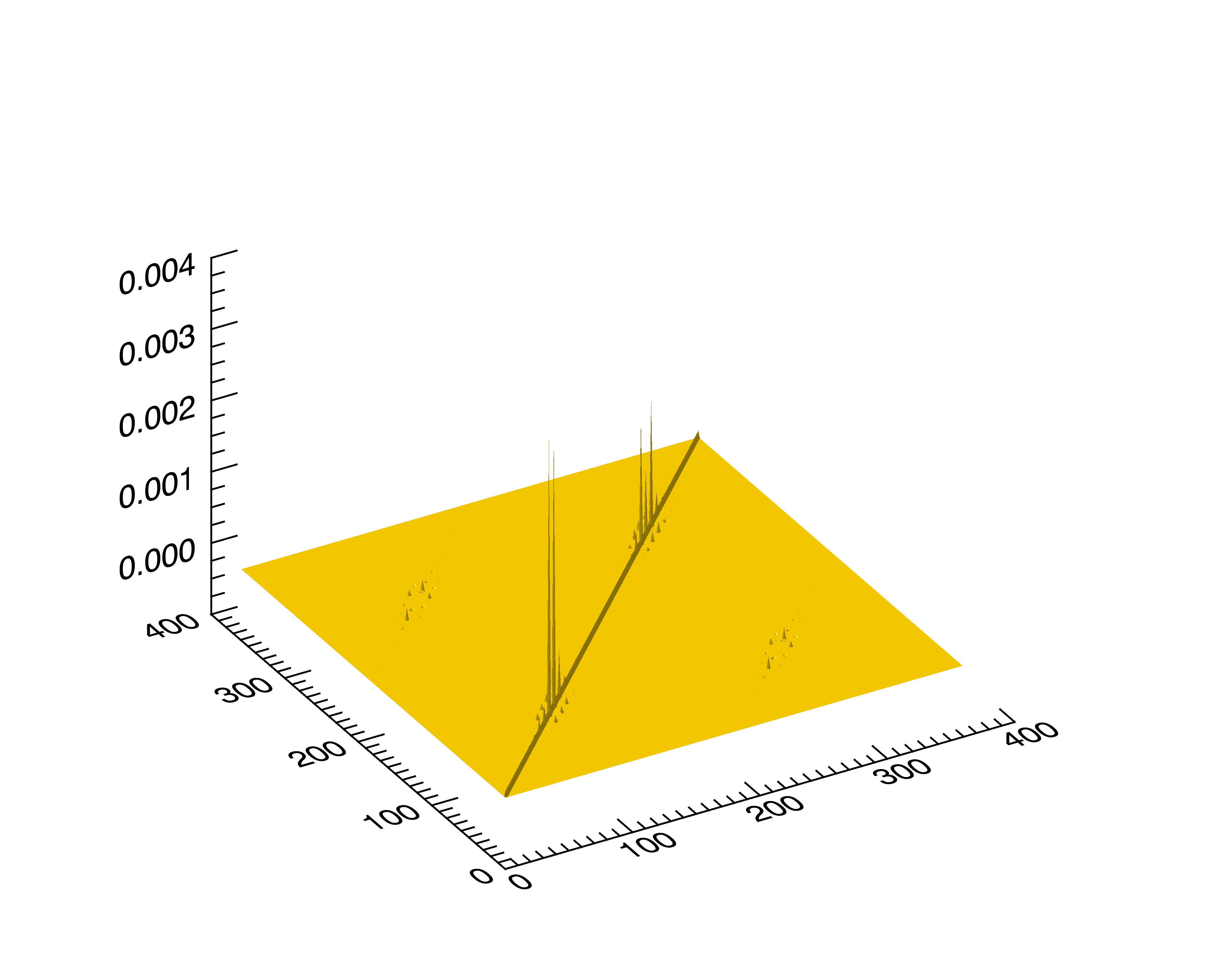
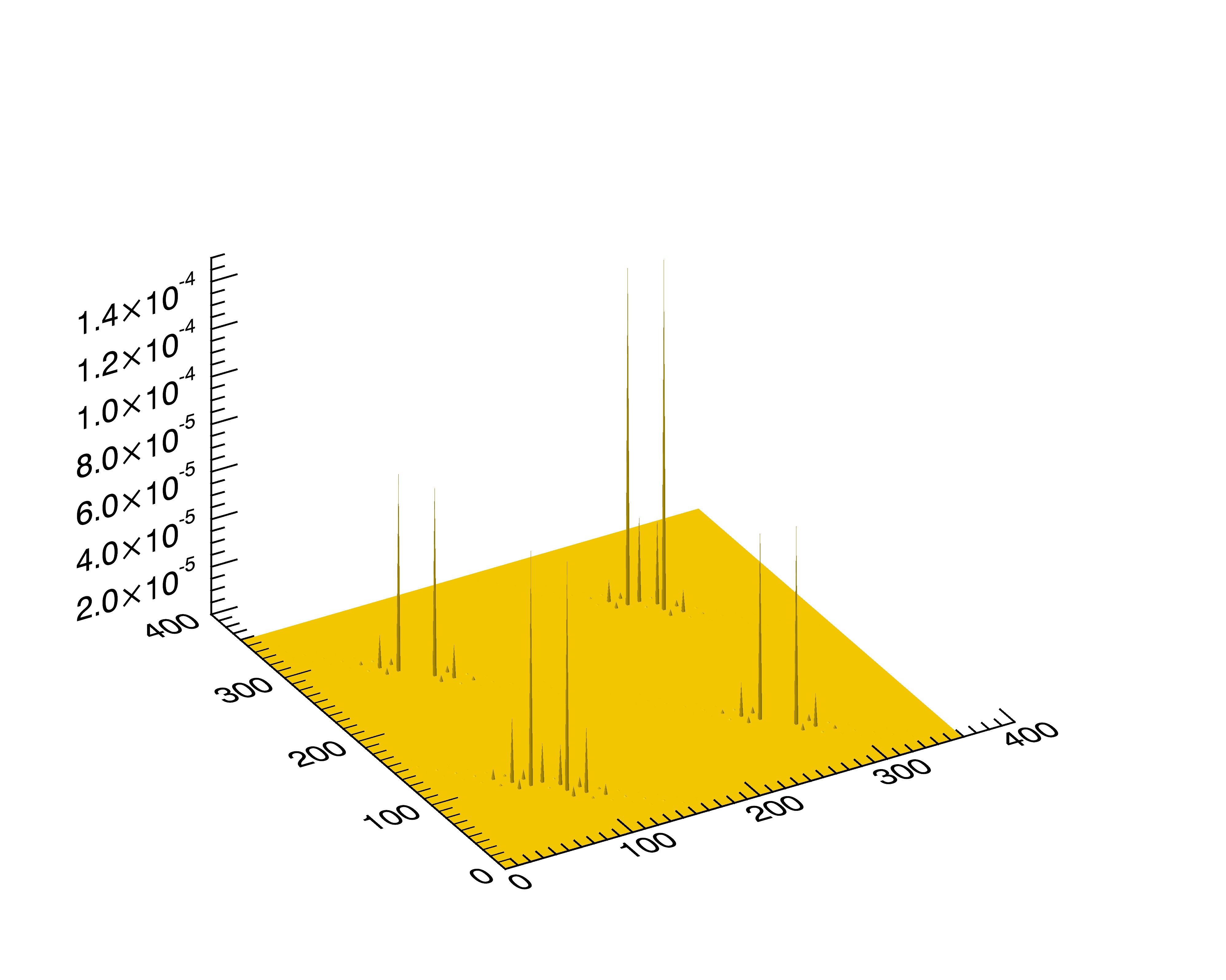
Figure 2: Covariance and relation matrices ๐šช๐šช{\boldsymbol{\Gamma}} and ๐‚๐‚\mathbf{C} for an array with Na=10subscript๐‘๐‘Ž10N_{a}=10, b=0.0873๐‘0.0873b=0.0873 rad, noise n=0.01โ€‹ฮผ๐‘›0.01๐œ‡n=0.01\,\muK. The sizes of both matrices are 360ร—360360360360\times 360 and the unit of the vertical axis is ฮผโ€‹K2๐œ‡superscriptK2\mu{\rm K}^{2}. Notice that noise only affects the ๐šช๐šช{\boldsymbol{\Gamma}} matrix.

II.3 Visibility Covariance Matrix and Fisher Matrix

We now apply the results of the previous section to visibility data. Suppose that our data consists of a set of visibilities cโ†’=(VQโ€‹(๐ฎ1),VQโ€‹(๐ฎ๐Ÿ),โ€ฆ,VUโ€‹(๐ฎ1),VUโ€‹(๐ฎ2),โ€ฆ)โ†’๐‘subscript๐‘‰๐‘„subscript๐ฎ1subscript๐‘‰๐‘„subscript๐ฎ2โ€ฆsubscript๐‘‰๐‘ˆsubscript๐ฎ1subscript๐‘‰๐‘ˆsubscript๐ฎ2โ€ฆ\vec{c}=(V_{Q}(\mathbf{u}_{1}),V_{Q}(\mathbf{u_{2}}),\ldots,V_{U}(\mathbf{u}_{1}),V_{U}(\mathbf{u}_{2}),\ldots). Consider an element of the upper left quadrant of the covariance matrix ๐šช๐šช{\boldsymbol{\Gamma}}, which is the covariance of two Q๐‘„Q visibilities. According to equations (8) and (II.1),

โŸจVQโ€‹(๐ฎ1)โ€‹VQโˆ—โ€‹(๐ฎ2)โŸฉdelimited-โŸจโŸฉsubscript๐‘‰๐‘„subscript๐ฎ1superscriptsubscript๐‘‰๐‘„subscript๐ฎ2\displaystyle\qquad\langle V_{Q}(\mathbf{u}_{1})V_{Q}^{*}(\mathbf{u}_{2})\rangle
=(2โ€‹ฯ€)2โ€‹โˆซโŸจQ~โ€‹(๐ค1)โ€‹Q~โˆ—โ€‹(๐ค2)โŸฉโ€‹A~โˆ—โ€‹(๐ค1+2โ€‹ฯ€โ€‹๐ฎ1)โ€‹A~โ€‹(๐ค2+2โ€‹ฯ€โ€‹๐ฎ2)โ€‹d2โ€‹๐คabsentsuperscript2๐œ‹2delimited-โŸจโŸฉ~๐‘„subscript๐ค1superscript~๐‘„subscript๐ค2superscript~๐ดsubscript๐ค12๐œ‹subscript๐ฎ1~๐ดsubscript๐ค22๐œ‹subscript๐ฎ2superscript๐‘‘2๐ค\displaystyle=(2\pi)^{2}\int{\langle\tilde{Q}(\mathbf{k}_{1})\tilde{Q}^{*}(\mathbf{k}_{2})\rangle}\tilde{A}^{*}(\mathbf{k}_{1}+2\pi\mathbf{u}_{1})\tilde{A}(\mathbf{k}_{2}+2\pi\mathbf{u}_{2})d^{2}\mathbf{k}
=(2ฯ€)2โˆซ(ฮด(๐ค1โˆ’๐ค2)[PE(๐ค)cos2(2ฯ•)+PB(๐ค)sin2(2ฯ•)]\displaystyle=(2\pi)^{2}\int{(\delta(\mathbf{k}_{1}-\mathbf{k}_{2})[P_{E}(\mathbf{k})\cos^{2}(2\phi)+P_{B}(\mathbf{k})\sin^{2}(2\phi)]}
A~โˆ—โ€‹(๐ค1+2โ€‹ฯ€โ€‹๐ฎ1)โ€‹A~โ€‹(๐ค2+2โ€‹ฯ€โ€‹๐ฎ2)โ€‹d2โ€‹๐คsuperscript~๐ดsubscript๐ค12๐œ‹subscript๐ฎ1~๐ดsubscript๐ค22๐œ‹subscript๐ฎ2superscript๐‘‘2๐ค\displaystyle\qquad\tilde{A}^{*}(\mathbf{k}_{1}+2\pi\mathbf{u}_{1})\tilde{A}(\mathbf{k}_{2}+2\pi\mathbf{u}_{2})d^{2}\mathbf{k}
=(2โ€‹ฯ€)2โ€‹โˆซ[PEโ€‹(๐ค)โ€‹cos2โก(2โ€‹ฯ•)+PBโ€‹(๐ค)โ€‹sin2โก(2โ€‹ฯ•)]absentsuperscript2๐œ‹2delimited-[]subscript๐‘ƒ๐ธ๐คsuperscript22italic-ฯ•subscript๐‘ƒ๐ต๐คsuperscript22italic-ฯ•\displaystyle=(2\pi)^{2}\int{[P_{E}(\mathbf{k})\cos^{2}(2\phi)+P_{B}(\mathbf{k})\sin^{2}(2\phi)]}
A~โˆ—โ€‹(๐ค+2โ€‹ฯ€โ€‹๐ฎ1)โ€‹A~โ€‹(๐ค+2โ€‹ฯ€โ€‹๐ฎ2)โ€‹d2โ€‹๐ค.superscript~๐ด๐ค2๐œ‹subscript๐ฎ1~๐ด๐ค2๐œ‹subscript๐ฎ2superscript๐‘‘2๐ค\displaystyle\qquad\tilde{A}^{*}(\mathbf{k}+2\pi\mathbf{u}_{1})\tilde{A}(\mathbf{k}+2\pi\mathbf{u}_{2})d^{2}\mathbf{k}. (41)

As long as A๐ดA is isotropic, this expression and the corresponding ones for โŸจVQโ€‹VUโˆ—โŸฉdelimited-โŸจโŸฉsubscript๐‘‰๐‘„superscriptsubscript๐‘‰๐‘ˆ\langle V_{Q}V_{U}^{*}\rangle and โŸจVUโ€‹VUโˆ—โŸฉdelimited-โŸจโŸฉsubscript๐‘‰๐‘ˆsuperscriptsubscript๐‘‰๐‘ˆ\langle V_{U}V_{U}^{*}\rangle can be expressed as a single integral by writing d2โ€‹ksuperscript๐‘‘2๐‘˜d^{2}k in polar coordinates and integrating over the angular coordinate, as shown in the Appendix.

As long as the antenna pattern A๐ดA has reflection symmetry, A~~๐ด\tilde{A} is real, and hence โŸจVQโ€‹(๐ฎ1)โ€‹VQโˆ—โ€‹(๐ฎ2)โŸฉdelimited-โŸจโŸฉsubscript๐‘‰๐‘„subscript๐ฎ1superscriptsubscript๐‘‰๐‘„subscript๐ฎ2\left<V_{Q}(\mathbf{u}_{1})V_{Q}^{*}(\mathbf{u}_{2})\right> is real as well. By similar reasoning, โŸจVQโ€‹(๐ฎ1)โ€‹VUโˆ—โ€‹(๐ฎ2)โŸฉdelimited-โŸจโŸฉsubscript๐‘‰๐‘„subscript๐ฎ1superscriptsubscript๐‘‰๐‘ˆsubscript๐ฎ2\left<V_{Q}(\mathbf{u}_{1})V_{U}^{*}(\mathbf{u}_{2})\right> and โŸจVUโ€‹(๐ฎ1)โ€‹VUโˆ—โ€‹(๐ฎ2)โŸฉdelimited-โŸจโŸฉsubscript๐‘‰๐‘ˆsubscript๐ฎ1superscriptsubscript๐‘‰๐‘ˆsubscript๐ฎ2\left<V_{U}(\mathbf{u}_{1})V_{U}^{*}(\mathbf{u}_{2})\right> are also real. Hence we conclude ๐šช๐šช{\boldsymbol{\Gamma}} is real for visibility data. The same is true for the relation matrix ๐‚๐‚\mathbf{C}.

Since ๐šชxโ€‹xsubscript๐šช๐‘ฅ๐‘ฅ{\boldsymbol{\Gamma}}_{xx}, ๐šชyโ€‹ysubscript๐šช๐‘ฆ๐‘ฆ{\boldsymbol{\Gamma}}_{yy}, ๐šชyโ€‹xsubscript๐šช๐‘ฆ๐‘ฅ{\boldsymbol{\Gamma}}_{yx} and ๐šชxโ€‹ysubscript๐šช๐‘ฅ๐‘ฆ{\boldsymbol{\Gamma}}_{xy} are all real, equations (30) and (31) imply that ๐šชyโ€‹xโˆ’๐šชxโ€‹y=๐šชyโ€‹x+๐šชxโ€‹y=0subscript๐šช๐‘ฆ๐‘ฅsubscript๐šช๐‘ฅ๐‘ฆsubscript๐šช๐‘ฆ๐‘ฅsubscript๐šช๐‘ฅ๐‘ฆ0{\boldsymbol{\Gamma}}_{yx}-{\boldsymbol{\Gamma}}_{xy}={\boldsymbol{\Gamma}}_{yx}+{\boldsymbol{\Gamma}}_{xy}=0, and hence that

๐šชyโ€‹xsubscript๐šช๐‘ฆ๐‘ฅ\displaystyle{\boldsymbol{\Gamma}}_{yx} =๐šชxโ€‹y=0,absentsubscript๐šช๐‘ฅ๐‘ฆ0\displaystyle={\boldsymbol{\Gamma}}_{xy}=0, (42)
๐šชxโ€‹xsubscript๐šช๐‘ฅ๐‘ฅ\displaystyle{\boldsymbol{\Gamma}}_{xx} =(๐šช+๐‚)/2,absent๐šช๐‚2\displaystyle=({\boldsymbol{\Gamma}}+\mathbf{C})/2, (43)
๐šชyโ€‹ysubscript๐šช๐‘ฆ๐‘ฆ\displaystyle{\boldsymbol{\Gamma}}_{yy} =(๐šชโˆ’๐‚)/2.absent๐šช๐‚2\displaystyle=({\boldsymbol{\Gamma}}-\mathbf{C})/2. (44)

Therefore, from the definition of ๐šช(r)superscript๐šช๐‘Ÿ{\boldsymbol{\Gamma}}^{(r)} (27), we see that ๐šช(r)superscript๐šช๐‘Ÿ{\boldsymbol{\Gamma}}^{(r)} is a block matrix

๐šช(r)=(๐šชxโ€‹x00๐šชyโ€‹y)=((๐šช+๐‚)/200(๐šชโˆ’๐‚)/2).superscript๐šช๐‘Ÿmatrixsubscript๐šช๐‘ฅ๐‘ฅ00subscript๐šช๐‘ฆ๐‘ฆmatrix๐šช๐‚200๐šช๐‚2{\boldsymbol{\Gamma}}^{(r)}=\begin{pmatrix}{\boldsymbol{\Gamma}}_{xx}&0\\ 0&{\boldsymbol{\Gamma}}_{yy}\end{pmatrix}=\begin{pmatrix}({\boldsymbol{\Gamma}}+\mathbf{C})/2&0\\ 0&({\boldsymbol{\Gamma}}-\mathbf{C})/2\end{pmatrix}. (45)

An example of ๐šช๐šช{\boldsymbol{\Gamma}} and ๐‚๐‚\mathbf{C} can be found in Figure 2.

Now we attain the final form for the visibility Fisher matrix

Fjโ€‹k=12subscript๐น๐‘—๐‘˜12\displaystyle F_{jk}={1\over 2} Trโ€‹((๐šชxโ€‹x)โˆ’1โ€‹dโ€‹๐šชxโ€‹xdโ€‹ฮธjโ€‹(๐šชxโ€‹x)โˆ’1โ€‹dโ€‹๐šชxโ€‹xdโ€‹ฮธk)Trsuperscriptsubscript๐šช๐‘ฅ๐‘ฅ1๐‘‘subscript๐šช๐‘ฅ๐‘ฅ๐‘‘subscript๐œƒ๐‘—superscriptsubscript๐šช๐‘ฅ๐‘ฅ1๐‘‘subscript๐šช๐‘ฅ๐‘ฅ๐‘‘subscript๐œƒ๐‘˜\displaystyle{\rm Tr}\left(({\boldsymbol{\Gamma}}_{xx})^{-1}{d{\boldsymbol{\Gamma}}_{xx}\over d\theta_{j}}({\boldsymbol{\Gamma}}_{xx})^{-1}{d{\boldsymbol{\Gamma}}_{xx}\over d\theta_{k}}\right)
+12โ€‹Trโ€‹((๐šชyโ€‹y)โˆ’1โ€‹dโ€‹๐šชyโ€‹ydโ€‹ฮธjโ€‹(๐šชyโ€‹y)โˆ’1โ€‹dโ€‹๐šชyโ€‹ydโ€‹ฮธk)12Trsuperscriptsubscript๐šช๐‘ฆ๐‘ฆ1๐‘‘subscript๐šช๐‘ฆ๐‘ฆ๐‘‘subscript๐œƒ๐‘—superscriptsubscript๐šช๐‘ฆ๐‘ฆ1๐‘‘subscript๐šช๐‘ฆ๐‘ฆ๐‘‘subscript๐œƒ๐‘˜\displaystyle+{1\over 2}{\rm Tr}\left(({\boldsymbol{\Gamma}}_{yy})^{-1}{d{\boldsymbol{\Gamma}}_{yy}\over d\theta_{j}}({\boldsymbol{\Gamma}}_{yy})^{-1}{d{\boldsymbol{\Gamma}}_{yy}\over d\theta_{k}}\right) (46)

II.4 The Augmented Fisher Matrix

The Fisher matrix allows us to compute the expected errors on cosmological parameters for an ideal experiment. We now want to introduce the possibility of sources of systematic error. Suppose that there is some imperfectly-known aspect of the experimental setup that can be characterized by a parameter p๐‘p. The experimenter has measured p๐‘p with some uncertainty, so that the probability density is sharply peaked around some measured value p^^๐‘\hat{p}. Often, we are willing to assume that the probability density fโ€‹(p|p^)๐‘“conditional๐‘^๐‘f(p|\hat{p}) is Gaussian with mean p^^๐‘\hat{p} and known variance ฯƒp2superscriptsubscript๐œŽ๐‘2\sigma_{p}^{2}.

Let us include the experimental parameter p๐‘p along with the cosmological parameters ฮธโ†’โ†’๐œƒ\vec{\theta} in the likelihood function:

Lโ€‹(ฮธโ†’,p)๐ฟโ†’๐œƒ๐‘\displaystyle L(\vec{\theta},p) โ‰กfโ€‹(rโ†’,p|ฮธโ†’,p^)=fโ€‹(rโ†’|ฮธโ†’,p)โ€‹fโ€‹(p|p^)absent๐‘“โ†’๐‘Ÿconditional๐‘โ†’๐œƒ^๐‘๐‘“conditionalโ†’๐‘Ÿโ†’๐œƒ๐‘๐‘“conditional๐‘^๐‘\displaystyle\equiv f(\vec{r},p|\vec{\theta},\hat{p})=f(\vec{r}|\vec{\theta},p)f(p|\hat{p})
=(expโก(โˆ’12โ€‹rโ†’Tโ€‹๐šชโˆ’1โ€‹rโ†’)(2โ€‹ฯ€)n/2โ€‹det1/2โ€‹(๐šช))โ€‹(expโก(โˆ’(pโˆ’p^)2/2โ€‹ฯƒp2)2โ€‹ฯ€โ€‹ฯƒp).absent12superscriptโ†’๐‘Ÿ๐‘‡superscript๐šช1โ†’๐‘Ÿsuperscript2๐œ‹๐‘›2superscriptdet12๐šชsuperscript๐‘^๐‘22superscriptsubscript๐œŽ๐‘22๐œ‹subscript๐œŽ๐‘\displaystyle=\left({\exp\left(-{1\over 2}\vec{r}^{T}{\boldsymbol{\Gamma}}^{-1}\vec{r}\right)\over(2\pi)^{n/2}{\rm det}^{1/2}({\boldsymbol{\Gamma}})}\right)\left({\exp(-(p-\hat{p})^{2}/2\sigma_{p}^{2})\over\sqrt{2\pi}\,\sigma_{p}}\right). (47)

In this expression, the covariance matrix ๐šช๐šช{\boldsymbol{\Gamma}} depends on both the cosmological parameters ฮธโ†’โ†’๐œƒ\vec{\theta} and the experimental parameter p๐‘p.

We want to determine the effect that our ignorance of p๐‘p has on our attempt to measure ฮธโ†’โ†’๐œƒ\vec{\theta}. We can do this by treating p๐‘p along with ฮธโ†’โ†’๐œƒ\vec{\theta} as unknowns to be estimated simultaneously and calculating an โ€œaugmentedโ€ Fisher matrix whose rows and columns correspond to the parameters ฮธโ†’(a)=(ฮธ1,ฮธ2,โ€ฆ,ฮธm,p)superscriptโ†’๐œƒ๐‘Žsubscript๐œƒ1subscript๐œƒ2โ€ฆsubscript๐œƒ๐‘š๐‘\vec{\theta}^{(a)}=(\theta_{1},\theta_{2},\ldots,\theta_{m},p).

The log-likelihood is given by

โ„’โ„’\displaystyle{\cal L} โ‰กโˆ’lnโกLabsent๐ฟ\displaystyle\equiv-\ln L
=12โ€‹(rโ†’Tโ€‹๐šชโˆ’1โ€‹rโ†’+lnโ€‹det๐šช+(pโˆ’p^)2ฯƒp2)+const.absent12superscriptโ†’๐‘Ÿ๐‘‡superscript๐šช1โ†’๐‘Ÿ๐šชsuperscript๐‘^๐‘2superscriptsubscript๐œŽ๐‘2const.\displaystyle={1\over 2}\left(\vec{r}^{T}{\boldsymbol{\Gamma}}^{-1}\vec{r}+\ln\det{\boldsymbol{\Gamma}}+{(p-\hat{p})^{2}\over\sigma_{p}^{2}}\right)+\mbox{const.} (48)

In calculating the Fisher matrix elements Fjโ€‹k=โˆ’โŸจโˆ‚2โ„’/โˆ‚ฮธj(a)โ€‹โˆ‚ฮธk(a)โŸฉsubscript๐น๐‘—๐‘˜delimited-โŸจโŸฉsuperscript2โ„’subscriptsuperscript๐œƒ๐‘Ž๐‘—subscriptsuperscript๐œƒ๐‘Ž๐‘˜F_{jk}=-\langle\partial^{2}{\cal L}/\partial\theta^{(a)}_{j}\partial\theta^{(a)}_{k}\rangle, the ensemble average in principle includes an average over all possible values of p^^๐‘\hat{p} as well as over all possible values of rโ†’โ†’๐‘Ÿ\vec{r}. However, it happens that all second derivatives of โ„’โ„’\cal L with respect to ฮธโ†’โ†’๐œƒ{\vec{\theta}} and p๐‘p are independent of p^^๐‘\hat{p}, so the averaging over p^^๐‘\hat{p} has no effect. Thus, the upper left mร—m๐‘š๐‘šm\times m block of the augmented Fisher matrix is still given by equation (46). All that remains is to determine the final row and column.

For jโ‰คm๐‘—๐‘šj\leq m we have

Fj,m+1=12โ€‹Trโ€‹((๐šช(r))โˆ’1โ€‹โˆ‚๐šช(r)โˆ‚ฮธjโ€‹(๐šช(r))โˆ’1โ€‹โˆ‚๐šช(r)โˆ‚p).subscript๐น๐‘—๐‘š112Trsuperscriptsuperscript๐šช๐‘Ÿ1superscript๐šช๐‘Ÿsubscript๐œƒ๐‘—superscriptsuperscript๐šช๐‘Ÿ1superscript๐šช๐‘Ÿ๐‘F_{j,m+1}={1\over 2}{\rm Tr}\left(({\boldsymbol{\Gamma}}^{(r)})^{-1}{\partial{\boldsymbol{\Gamma}}^{(r)}\over\partial\theta_{j}}({\boldsymbol{\Gamma}}^{(r)})^{-1}{\partial{\boldsymbol{\Gamma}}^{(r)}\over\partial p}\right). (49)

Note that this is just the usual Fisher matrix element, treating p๐‘p as a normal cosmological parameter. The very last term, in the lower right corner has an extra 1/ฯƒp21superscriptsubscript๐œŽ๐‘21/{\sigma_{p}^{2}} in it

Fm+1,m+1=12โ€‹Trโ€‹((๐šช(r))โˆ’1โ€‹โˆ‚๐šช(r)โˆ‚pโ€‹(๐šช(r))โˆ’1โ€‹โˆ‚๐šช(r)โˆ‚p)+1ฯƒp2,subscript๐น๐‘š1๐‘š112Trsuperscriptsuperscript๐šช๐‘Ÿ1superscript๐šช๐‘Ÿ๐‘superscriptsuperscript๐šช๐‘Ÿ1superscript๐šช๐‘Ÿ๐‘1superscriptsubscript๐œŽ๐‘2F_{m+1,m+1}={1\over 2}{\rm Tr}\left(({\boldsymbol{\Gamma}}^{(r)})^{-1}{\partial{\boldsymbol{\Gamma}}^{(r)}\over\partial p}({\boldsymbol{\Gamma}}^{(r)})^{-1}{\partial{\boldsymbol{\Gamma}}^{(r)}\over\partial p}\right)+{1\over\sigma_{p}^{2}}, (50)

arising from the term (pโˆ’p^)2/ฯƒp2superscript๐‘^๐‘2superscriptsubscript๐œŽ๐‘2(p-\hat{p})^{2}/\sigma_{p}^{2} in equation (48).

In the formulae above we have assumed that we only have one systematic parameter. The generalization to n๐‘›n parameters is straightforward, leading to an (m+n)ร—(m+n)๐‘š๐‘›๐‘š๐‘›(m+n)\times(m+n) augmented Fisher matrix.

II.5 Rotation errors

In section IV, we consider two examples of systematic errors: gain errors and rotation errors. In order to assess the effect of these errors on power spectrum estimates, we need to know their effects on the visibility covariance matrix. The case of gain errors is trivial: a gain error g๐‘”g on a given antenna multiplies all of the micro-visibilities involving that antenna by 1+g1๐‘”1+g. The case of rotation errors requires more attention.

Suppose that each antenna j๐‘—j has its polarizers rotated by some unknown angle pjsubscript๐‘๐‘—p_{j}, with corresponding rotation matrix ๐‘j=๐‘โ€‹(pj)subscript๐‘๐‘—๐‘subscript๐‘๐‘—{\bf R}_{j}={\bf R}(p_{j}). Consider a measurement of a micro-visibility pair (VQ,(aโ€‹b),VU,(aโ€‹b))subscript๐‘‰๐‘„๐‘Ž๐‘subscript๐‘‰๐‘ˆ๐‘Ž๐‘(V_{Q,(ab)},V_{U,(ab)}), where (aโ€‹b)๐‘Ž๐‘(ab) labels an atenna pair. Then the observed Stokes matrix ๐’๐’{\bf S} of (4) is related to the true (error-free) matrix ๐’^^๐’\hat{\bf S} as

๐’=๐‘aโ€‹๐’^โ€‹๐‘bโ€ .๐’subscript๐‘๐‘Ž^๐’superscriptsubscript๐‘๐‘โ€ {\bf S}={\bf R}_{a}\hat{\bf S}{\bf R}_{b}^{\dagger}. (51)

Because the visibilities are linearly related to the matrix ๐’๐’{\bf S}, they obey a similar rule:

๐•=๐‘aโ€‹๐•^โ€‹๐‘bโ€ ๐•subscript๐‘๐‘Ž^๐•superscriptsubscript๐‘๐‘โ€ {\bf V}={\bf R}_{a}\hat{\bf V}{\bf R}_{b}^{\dagger} (52)

Applying the rotation matrices to the Stokes visibility matrix, we find that

VQโ€‹(aโ€‹b)subscript๐‘‰๐‘„๐‘Ž๐‘\displaystyle V_{Q(ab)} =V^Qโ€‹(aโ€‹b)โ€‹cosโก(pa+pb)+V^Uโ€‹(aโ€‹b)โ€‹sinโก(pa+pb),absentsubscript^๐‘‰๐‘„๐‘Ž๐‘subscript๐‘๐‘Žsubscript๐‘๐‘subscript^๐‘‰๐‘ˆ๐‘Ž๐‘subscript๐‘๐‘Žsubscript๐‘๐‘\displaystyle=\hat{V}_{Q(ab)}\cos(p_{a}+p_{b})+\hat{V}_{U(ab)}\sin(p_{a}+p_{b}), (53)
VUโ€‹(aโ€‹b)subscript๐‘‰๐‘ˆ๐‘Ž๐‘\displaystyle V_{U(ab)} =โˆ’V^Qโ€‹(aโ€‹b)โ€‹sinโก(pa+pb)+V^Uโ€‹(aโ€‹b)โ€‹cosโก(pa+pb).absentsubscript^๐‘‰๐‘„๐‘Ž๐‘subscript๐‘๐‘Žsubscript๐‘๐‘subscript^๐‘‰๐‘ˆ๐‘Ž๐‘subscript๐‘๐‘Žsubscript๐‘๐‘\displaystyle=-\hat{V}_{Q(ab)}\sin(p_{a}+p_{b})+\hat{V}_{U(ab)}\cos(p_{a}+p_{b}). (54)

That is, the visibilities (VQโ€‹(aโ€‹b)VUโ€‹(aโ€‹b))matrixsubscript๐‘‰๐‘„๐‘Ž๐‘subscript๐‘‰๐‘ˆ๐‘Ž๐‘\begin{pmatrix}V_{Q(ab)}\\ V_{U(ab)}\end{pmatrix} are simply multiplied by the rotation matrix corresponding to (pa+pb)subscript๐‘๐‘Žsubscript๐‘๐‘(p_{a}+p_{b}).

Now consider the covariance between two pairs of macro-visibilities VXโ€‹Jsubscript๐‘‰๐‘‹๐ฝV_{XJ} and VXโ€‹Ksubscript๐‘‰๐‘‹๐พV_{XK}, where Xโˆˆ{Q,U}๐‘‹๐‘„๐‘ˆX\in\{Q,U\} and J,K๐ฝ๐พJ,K label the visibilities. We can express their covariances as a 2ร—2222\times 2 submatrix of the full covariance matrix:

๐‚=โŸจ๐ฏJโ€‹๐ฏKโ€ โŸฉ,๐‚delimited-โŸจโŸฉsubscript๐ฏ๐ฝsuperscriptsubscript๐ฏ๐พโ€ {\bf C}=\left<{\bf v}_{J}{\bf v}_{K}^{\dagger}\right>, (55)

where

๐ฏJ=(VQโ€‹JVUโ€‹J).subscript๐ฏ๐ฝmatrixsubscript๐‘‰๐‘„๐ฝsubscript๐‘‰๐‘ˆ๐ฝ{\bf v}_{J}=\begin{pmatrix}V_{QJ}\\ V_{UJ}\end{pmatrix}. (56)

In the absence of systematic errors, the covariance matrix is

๐‚๐ŸŽ=1NJโ€‹NKโ€‹โˆ‘(aโ€‹b)โˆˆSJโˆ‘(cโ€‹d)โˆˆSKโŸจ๐ฏ(aโ€‹b)โ€‹๐ฏ(cโ€‹d)โ€ โŸฉsubscript๐‚01subscript๐‘๐ฝsubscript๐‘๐พsubscript๐‘Ž๐‘subscript๐‘†๐ฝsubscript๐‘๐‘‘subscript๐‘†๐พdelimited-โŸจโŸฉsubscript๐ฏ๐‘Ž๐‘superscriptsubscript๐ฏ๐‘๐‘‘โ€ {\bf C_{0}}={1\over N_{J}N_{K}}\sum_{(ab)\in S_{J}}\sum_{(cd)\in S_{K}}\left<{\bf v}_{(ab)}{\bf v}_{(cd)}^{\dagger}\right> (57)

As we saw above, each micro-visibility is modified as follows:

๐ฏ(aโ€‹b)โ†’๐‘aโ€‹๐‘bโ€‹๐ฏ(aโ€‹b).โ†’subscript๐ฏ๐‘Ž๐‘subscript๐‘๐‘Žsubscript๐‘๐‘subscript๐ฏ๐‘Ž๐‘{\bf v}_{(ab)}\to{\bf R}_{a}{\bf R}_{b}{\bf v}_{(ab)}. (58)

The 2ร—2222\times 2 covariance matrix corresponding to macro-visibilities J,K๐ฝ๐พJ,K is therefore

๐‚๐‚\displaystyle{\bf C} =1NJโ€‹NKโ€‹โˆ‘(aโ€‹b)โˆˆSJโˆ‘(cโ€‹d)โˆˆSKโŸจ๐ฏ(aโ€‹b)โ€‹๐ฏ(cโ€‹d)โ€ โŸฉabsent1subscript๐‘๐ฝsubscript๐‘๐พsubscript๐‘Ž๐‘subscript๐‘†๐ฝsubscript๐‘๐‘‘subscript๐‘†๐พdelimited-โŸจโŸฉsubscript๐ฏ๐‘Ž๐‘superscriptsubscript๐ฏ๐‘๐‘‘โ€ \displaystyle={1\over N_{J}N_{K}}\sum_{(ab)\in S_{J}}\sum_{(cd)\in S_{K}}\left<{\bf v}_{(ab)}{\bf v}_{(cd)}^{\dagger}\right>
=1NJโ€‹NKโ€‹โˆ‘(aโ€‹b)โˆˆSJโˆ‘(cโ€‹d)โˆˆSK๐‘aโ€‹๐‘bโ€‹๐‚0โ€‹๐‘dโ€ โ€‹๐‘cโ€ absent1subscript๐‘๐ฝsubscript๐‘๐พsubscript๐‘Ž๐‘subscript๐‘†๐ฝsubscript๐‘๐‘‘subscript๐‘†๐พsubscript๐‘๐‘Žsubscript๐‘๐‘subscript๐‚0superscriptsubscript๐‘๐‘‘โ€ superscriptsubscript๐‘๐‘โ€ \displaystyle={1\over N_{J}N_{K}}\sum_{(ab)\in S_{J}}\sum_{(cd)\in S_{K}}{\bf R}_{a}{\bf R}_{b}{\bf C}_{0}{\bf R}_{d}^{\dagger}{\bf R}_{c}^{\dagger}
=(1NJโ€‹โˆ‘(aโ€‹b)โˆˆSJ๐‘aโ€‹๐‘b)โ€‹๐‚0โ€‹(1NKโ€‹โˆ‘(cโ€‹d)โˆˆSK๐‘cโ€‹๐‘d)โ€ absent1subscript๐‘๐ฝsubscript๐‘Ž๐‘subscript๐‘†๐ฝsubscript๐‘๐‘Žsubscript๐‘๐‘subscript๐‚0superscript1subscript๐‘๐พsubscript๐‘๐‘‘subscript๐‘†๐พsubscript๐‘๐‘subscript๐‘๐‘‘โ€ \displaystyle=\left({1\over N_{J}}\sum_{(ab)\in S_{J}}{\bf R}_{a}{\bf R}_{b}\right){\bf C}_{0}\left({1\over N_{K}}\sum_{(cd)\in S_{K}}{\bf R}_{c}{\bf R}_{d}\right)^{\dagger}
=โ„›Jโ€‹๐‚0โ€‹โ„›Kโ€ ,absentsubscriptโ„›๐ฝsubscript๐‚0superscriptsubscriptโ„›๐พโ€ \displaystyle={\cal R}_{J}{\bf C}_{0}{\cal R}_{K}^{\dagger}, (59)

where the matrices โ„›โ„›{\cal R} are defined by the last line.

We can apply this rule to each pair of macro-visibilities to determine the effect of the rotation errors on the entire visibility covariance matrix.

III Approximate analytic treatment

Bunn Bunn (2007) gave an approximate analytic treatment of various sources of systematic errors in CMB interferometry. We will compare the full Fisher matrix calculation described above to this treatment. In this section, we briefly review and extend the methods outlined in that paper.

III.1 Statistical errors on power spectrum estimates

Before introducing systematic errors, we present a simple method for estimating purely statistical errors on power spectrum estimates.

Following Bunn (2007), we begin by imagining an experiment that measures only a single visiblity pair (VQ,VU)subscript๐‘‰๐‘„subscript๐‘‰๐‘ˆ(V_{Q},V_{U}). According to equation (4.8b) of Bunn (2007), for a single visibility pair, we can find an unbiased estimator of ClBsuperscriptsubscript๐ถ๐‘™๐ตC_{l}^{B} in a band centered on l=2โ€‹ฯ€โ€‹u๐‘™2๐œ‹๐‘ขl=2\pi u,

C^B,single=(ฯ€โ€‹b2)โˆ’1โ€‹ฮณโ€‹(c2ยฏโ€‹|VU|2โˆ’s2ยฏโ€‹|VQ|2),subscript^๐ถ๐ตsinglesuperscript๐œ‹superscript๐‘21๐›พยฏsuperscript๐‘2superscriptsubscript๐‘‰๐‘ˆ2ยฏsuperscript๐‘ 2superscriptsubscript๐‘‰๐‘„2\hat{C}_{B,\rm single}=(\pi b^{2})^{-1}\gamma(\overline{c^{2}}\lvert V_{U}\rvert^{2}-\overline{s^{2}}\lvert V_{Q}\rvert^{2}), (60)

where b๐‘b is the beam size,

ฮณ=[(c2ยฏ)2โˆ’(s2ยฏ)2]โˆ’1,๐›พsuperscriptdelimited-[]superscriptยฏsuperscript๐‘22superscriptยฏsuperscript๐‘ 221\gamma=[(\overline{c^{2}})^{2}-(\overline{s^{2}})^{2}]^{-1}, (61)

and

c2ยฏยฏsuperscript๐‘2\displaystyle\overline{c^{2}} =โˆซ|A2~โ€‹(๐ค+2โ€‹ฯ€โ€‹๐ฎ)|2โ€‹cos2โก(ฯ•)โ€‹d2โ€‹๐คโˆซ|A2~(๐ค+2ฯ€๐ฎ)|2d2๐ค\displaystyle=\frac{\int{\lvert\tilde{A^{2}}(\mathbf{k}+2\pi\mathbf{u}})\rvert^{2}\cos^{2}(\phi)d^{2}\mathbf{k}}{\int{\lvert\tilde{A^{2}}(\mathbf{k}+2\pi\mathbf{u}})\lvert^{2}d^{2}\mathbf{k}} (62)
s2ยฏยฏsuperscript๐‘ 2\displaystyle\overline{s^{2}} =โˆซ|A2~โ€‹(๐ค+2โ€‹ฯ€โ€‹๐ฎ)|2โ€‹sin2โก(ฯ•)โ€‹d2โ€‹๐คโˆซ|A2~(๐ค+2ฯ€๐ฎ)|2d2๐ค=1โˆ’c2ยฏ\displaystyle=\frac{\int{\lvert\tilde{A^{2}}(\mathbf{k}+2\pi\mathbf{u}})\rvert^{2}\sin^{2}(\phi)d^{2}\mathbf{k}}{\int{\lvert\tilde{A^{2}}(\mathbf{k}+2\pi\mathbf{u}})\lvert^{2}d^{2}\mathbf{k}}=1-\overline{c^{2}} (63)

We have defined ฮธBsubscript๐œƒ๐ต\theta_{B} as the ratio of measured to true power, so the estimator of this quantity is ฮธ^B,single=C^B/CBsubscript^๐œƒ๐ตsinglesubscript^๐ถ๐ตsubscript๐ถ๐ต\hat{\theta}_{B,\rm single}=\hat{C}_{B}/C_{B}. After some algebra, we find that the variance of ฮธB,singlesubscript๐œƒ๐ตsingle\theta_{B,\rm single} is

ฯƒB,single2superscriptsubscript๐œŽ๐ตsingle2\displaystyle\sigma_{B,\rm single}^{2} =โŸจฮธ^B,single2โŸฉโˆ’โŸจฮธ^B,singleโŸฉ2absentdelimited-โŸจโŸฉsuperscriptsubscript^๐œƒ๐ตsingle2superscriptdelimited-โŸจโŸฉsubscript^๐œƒ๐ตsingle2\displaystyle=\langle\hat{\theta}_{B,\rm single}^{2}\rangle-\langle\hat{\theta}_{B,\rm single}\rangle^{2}
=ฮณ2[2(c2ยฏ)2(s2ยฏ)2(CECB)2+((c2ยฏ)4+(s2ยฏ)4)\displaystyle=\gamma^{2}\left[2(\overline{c^{2}})^{2}(\overline{s^{2}})^{2}\left(\frac{C_{E}}{C_{B}}\right)^{2}+((\overline{c^{2}})^{4}+(\overline{s^{2}})^{4})\right.
+(2(c2ยฏ)3s2ยฏ+2(s2ยฏ)3c2ยฏ)(CECB)]\displaystyle\left.+(2(\overline{c^{2}})^{3}\overline{s^{2}}+2(\overline{s^{2}})^{3}\overline{c^{2}})\left(\frac{C_{E}}{C_{B}}\right)\right] (64)

We now consider an experiment with many measured macro-visibilities, and regard each macro-visibility pair as an independent measurement of ฮธBsubscript๐œƒ๐ต\theta_{B}. Then the minimum-variance estimator from the entire data set is the usual weighted average, with weights given by the inverse variance, and the variance of this estimator is

ฯƒB,final2=(โˆ‘JฯƒBโ€‹Jโˆ’2)โˆ’1,superscriptsubscript๐œŽ๐ตfinal2superscriptsubscript๐ฝsuperscriptsubscript๐œŽ๐ต๐ฝ21\sigma_{B,\rm final}^{2}=\left(\sum_{J}\sigma_{BJ}^{-2}\right)^{-1}, (65)

where ฯƒBโ€‹J2superscriptsubscript๐œŽ๐ต๐ฝ2\sigma_{BJ}^{2} is given by (64) for baseline J๐ฝJ.

In Section IV, we will compare the results of this simple approximation with the full Fisher matrix calculation, as well as with the approximation in which calculate the fisher matrix while keeping only diagonal elements of the (real) covariance matrix.

III.2 Systematic errors

We now summarize the key results of Bunn (2007). Once again, we begin by imagining measurements of the intensity and polarization visibilities, ๐ฏโ‰ก(VI,VQ,VU)T๐ฏsuperscriptsubscript๐‘‰๐ผsubscript๐‘‰๐‘„subscript๐‘‰๐‘ˆ๐‘‡{\bf v}\equiv(V_{I},V_{Q},V_{U})^{T} for a single baseline. In many cases, the leading-order effect of a systematic error is to โ€œmixโ€ the visibilities, inducing errors ฮดโ€‹๐ฏ=๐„โ‹…๐ฏ๐›ฟ๐ฏโ‹…๐„๐ฏ\delta{\bf v}={\bf E}\cdot{\bf v} for some mixing matrix ๐„๐„{\bf E}.

Refer to caption
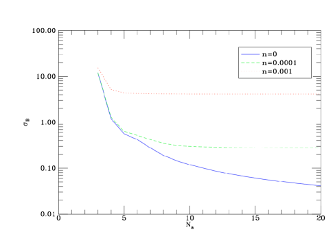
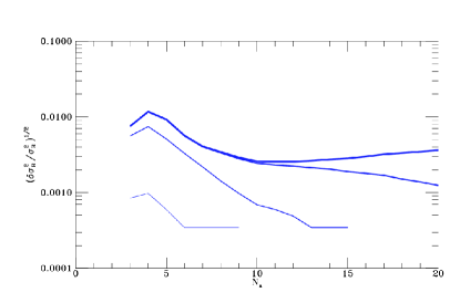
Figure 3: The relation between ฯƒBsubscript๐œŽ๐ต\sigma_{B} and Nasubscript๐‘๐‘ŽN_{a} for noise levels 0, 0.0001โ€‰ฮผ๐œ‡\muK, and 0.001โ€‰ฮผ๐œ‡\muK. The beam size b=0.0873๐‘0.0873b=0.0873 rad.

If the experimenter then uses the data set ๐ฏ๐ฏ{\bf v} to optimally estimate the E and B power spectra, without accounting for the effect of the systematic error, then the resulting estimates will have errors given by

(ฮดโ€‹C^rmsK)2=p2โ€‹โˆ‘I,JฮบK,Iโ€‹J2โ€‹CIโ€‹CJ,superscript๐›ฟsuperscriptsubscript^๐ถrms๐พ2superscript๐‘2subscript๐ผ๐ฝsubscriptsuperscript๐œ…2๐พ๐ผ๐ฝsuperscript๐ถ๐ผsuperscript๐ถ๐ฝ\left({\delta\hat{C}_{\rm rms}^{K}}\right)^{2}=p^{2}\sum_{I,J}\kappa^{2}_{K,IJ}{C^{I}C^{J}}, (66)

where I,J,Kโˆˆ{T,X,E,B}๐ผ๐ฝ๐พ๐‘‡๐‘‹๐ธ๐ตI,J,K\in\{T,X,E,B\} label the power spectra (temperature, TE correlation, E polarization, B polarization), p๐‘p is the rms amplitude of the error under consideration, and the coefficients ฮบK,Iโ€‹Jsubscript๐œ…๐พ๐ผ๐ฝ\kappa_{K,IJ} can be calculated from the error mixing matrix ๐„๐„{\bf E}. Because there is a hierarchy in power spectrum amplitudes, with T>X>E>B๐‘‡๐‘‹๐ธ๐ตT>X>E>B, one can generally keep only the dominant term in this sum.
Refer to caption
Refer to caption
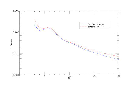
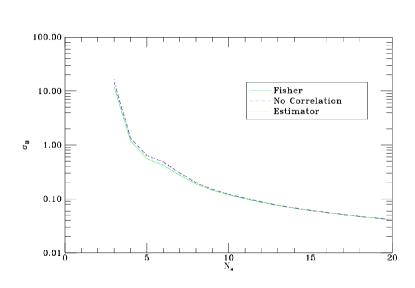
Figure 4: The relationship between ฯƒBsubscript๐œŽ๐ต\sigma_{B} and Nasubscript๐‘๐‘ŽN_{a} in the absence of systematic errors, calculated via the full Fisher matrix, the Fisher matrix with correlations between distinct baselines neglected, and the analytic estimator ฮธ^Bsubscript^๐œƒ๐ต\hat{\theta}_{B} of Section III. The left panel shows the errors calculated by the three methods, and the right shows the difference (74) between the approximations and the full Fisher calculations. Noise is set to zero in these calculations.

For example, for gain errors, the dominant term in the B power spectrum error is the one that corresponds to contamination by E power, with

ฮบB,Eโ€‹E2=2โ€‹ฮณ2โ€‹(s2ยฏโ€‹c2ยฏ)2subscriptsuperscript๐œ…2๐ต๐ธ๐ธ2superscript๐›พ2superscriptยฏsuperscript๐‘ 2ยฏsuperscript๐‘22\kappa^{2}_{B,EE}=2\gamma^{2}(\overline{s^{2}}\,\overline{c^{2}})^{2} (67)

As in the case of statistical errors above, we can crudely estimate the expected effect of a systematic error in a many-baseline experiment by assuming that each baseline provides an independent power spectrum estimate and performing an appropriate average. See Section V of Bunn (2007) for details.

Equation (65) gives the analytic approximation for ฯƒBsubscript๐œŽ๐ต\sigma_{B} in the absence of systematic errors. In generalizing it to the case where a systematic error is included, we assume that, for each antenna, the error caused by the systematic error p๐‘p is independent of the statistical error, so that

ฯƒBโ€‹j2=ฯƒBโ€‹j,02+ฯƒBโ€‹j,p2.superscriptsubscript๐œŽ๐ต๐‘—2superscriptsubscript๐œŽ๐ต๐‘—02superscriptsubscript๐œŽ๐ต๐‘—๐‘2\sigma_{Bj}^{2}=\sigma_{Bj,0}^{2}+\sigma_{Bj,p}^{2}. (68)

Here ฯƒBโ€‹jsubscript๐œŽ๐ต๐‘—\sigma_{Bj} is the error on the B power spectrum estimate corresponding to the j๐‘—jth micro-visibility. The quantity ฯƒBโ€‹j,02superscriptsubscript๐œŽ๐ต๐‘—02\sigma_{Bj,0}^{2} is the noise variance for that visibility in the absence of systematic errors, given by equation (64), and ฯƒBโ€‹j,p2=(ฮดโ€‹C^rmsB)2/ClBsuperscriptsubscript๐œŽ๐ต๐‘—๐‘2superscript๐›ฟsubscriptsuperscript^๐ถ๐ตrms2superscriptsubscript๐ถ๐‘™๐ต\sigma_{Bj,p}^{2}=(\delta\hat{C}^{B}_{\rm rms})^{2}/C_{l}^{B} is the additional variance induced by the systematic error. (Here l=2โ€‹ฯ€โ€‹u๐‘™2๐œ‹๐‘ขl=2\pi u for the given visibility.) Because each macro-visibility is estimated via an average of the corresponding micro-visibilities, we can compute the expected error in our B power spectrum estimate for each macro-visibility. The final error on the B power is then given by equation (65).

IV Results

We have calculated Fisher matrix errors for Naร—Nasubscript๐‘๐‘Žsubscript๐‘๐‘ŽN_{a}\times N_{a} square arrays of close-packed antennas with Gaussian beam width b=5โˆ˜=0.0873๐‘superscript50.0873b=5^{\circ}=0.0873 rad, as in Zhang etย al. (2013). We assume that the input power spectra are given by the standard LCDM model Planck Collaboration etย al. (2014) with tensor-to-scalar ratio r=0.1๐‘Ÿ0.1r=0.1, and that the experimenterโ€™s goal is to estimate the amplitudes of the E and B power spectra. To be specific, let CE,CBsuperscript๐ถ๐ธsuperscript๐ถ๐ตC^{E},C^{B} be the true power spectra. Then the parameters to be estimated are ฮธE,ฮธBsubscript๐œƒ๐ธsubscript๐œƒ๐ต\theta_{E},\theta_{B} such that the estimated power spectra are

C^Esuperscript^๐ถ๐ธ\displaystyle\hat{C}^{E} =ฮธEโ€‹CEabsentsubscript๐œƒ๐ธsuperscript๐ถ๐ธ\displaystyle=\theta_{E}C^{E} (69)
C^Bsuperscript^๐ถ๐ต\displaystyle\hat{C}^{B} =ฮธBโ€‹CBabsentsubscript๐œƒ๐ตsuperscript๐ถ๐ต\displaystyle=\theta_{B}C^{B} (70)

Since ฮธE,ฮธBsubscript๐œƒ๐ธsubscript๐œƒ๐ต\theta_{E},\theta_{B} are defined as relative amplitudes, their true value is one. The errors computed for these quantities will therefore be relative errors on the amplitude of the E and B signals. It would be straightforward to generalize these results to the estimation of multiple band powers in E and B.

We are particularly interested in the detectability of the faint B signal. As a result, we will focus on the quantity ฯƒB=(Fโˆ’1)Bโ€‹Bsubscript๐œŽ๐ตsubscriptsuperscript๐น1๐ต๐ต\sigma_{B}=\sqrt{(F^{-1})_{BB}}, which is the standard deviation of ฮธBsubscript๐œƒ๐ต\theta_{B} if none of the other parameters is known.

IV.1 Exact Fisher Matrix with different noise levels

We begin by ignoring all systematic errors and focusing on the effect of noise levels on the Fisher matrix. Assuming that all visibilities are subjected to white noise with standard deviation n๐‘›n, the visibility covariance matrix is

๐šชnโ€‹oโ€‹iโ€‹sโ€‹e=๐šช+n2โ€‹๐ˆ,subscript๐šช๐‘›๐‘œ๐‘–๐‘ ๐‘’๐šชsuperscript๐‘›2๐ˆ{\boldsymbol{\Gamma}}_{noise}={\boldsymbol{\Gamma}}+n^{2}\mathbf{I}, (71)

where ๐ˆ๐ˆ\mathbf{I} is the identity matrix.

Figure 3 shows the relationship between ฯƒBsubscript๐œŽ๐ต\sigma_{B} and Nasubscript๐‘๐‘ŽN_{a} for noise levels n=0๐‘›0n=0, 0.0001, and 0.001 ฮผ๐œ‡\muK.111If these values seem surprisingly small, note that, with our Fourier transform and antenna pattern normalization conventions, the variance of a visibility is โˆผฯ€โ€‹b2โ€‹ClEsimilar-toabsent๐œ‹superscript๐‘2superscriptsubscript๐ถ๐‘™๐ธ\sim\pi b^{2}C_{l}^{E}. For noise-free experiments, ฯƒBsubscript๐œŽ๐ต\sigma_{B} gradually decreases as Nasubscript๐‘๐‘ŽN_{a} increases. However, when some noise is present, there is a limit for Nasubscript๐‘๐‘ŽN_{a} at which ฯƒBsubscript๐œŽ๐ต\sigma_{B} cannot be attenuated even if we continue to increase the number of antennas.

For further analysis, we set n=0.0002โ€‹ฮผ๐‘›0.0002๐œ‡n=0.0002\,\muK, a value which allows for a detection of B modes but for which noise contributions are still significant.

IV.2 Comparison of calculation methods

In this section, we compare errors calculated using the full Fisher matrix formalism with those based on two approximate methods. One is the analytic approximations described in III. The other is a Fisher-matrix calculation, with the approximation that off-diagonal correlations between visibilities can be neglected โ€“ that is, that ฮ“jโ€‹k(r)=0subscriptsuperscriptฮ“๐‘Ÿ๐‘—๐‘˜0\Gamma^{(r)}_{jk}=0 for all (j,k)๐‘—๐‘˜(j,k) corresponding to macro-visibilities with distinct baselines ๐ฎjโ‰ ๐ฎksubscript๐ฎ๐‘—subscript๐ฎ๐‘˜{\bf u}_{j}\neq{\bf u}_{k}.

We begin by considering purely statistical errors and then introduce systematic errors.

IV.2.1 Statistical errors

We do not consider systematic errors in this section, meaning that our Fisher matrix will only be a 2ร—2222\times 2 matrix, corresponding to the two cosmological parameters ฮธE,ฮธBsubscript๐œƒ๐ธsubscript๐œƒ๐ต\theta_{E},\theta_{B} to be estimated. One example of a typical Fisher matrix is

F=(1794.234.233.08)๐นmatrix1794.234.233.08F=\begin{pmatrix}179&4.23\\ 4.23&3.08\end{pmatrix} (72)

with inverse

Fโˆ’1=(0.00577โˆ’0.00792โˆ’0.007920.33586797)superscript๐น1matrix0.005770.007920.007920.33586797F^{-1}=\begin{pmatrix}0.00577&-0.00792\\ -0.00792&0.33586797\end{pmatrix} (73)

with the parameters Na=10subscript๐‘๐‘Ž10N_{a}=10, beam size b=0.0873๐‘0.0873b=0.0873 rad, and n=0.0002โ€‹ฮผ๐‘›0.0002๐œ‡n=0.0002\,\muK. (We give extra significant figures for the ฯƒBsubscript๐œŽ๐ต\sigma_{B} term for comparison with later results.) This matrix indicates, for instance, that with the given parameters the least possible variance for measuring ฮธBsubscript๐œƒ๐ต\theta_{B} is 0.3360.3360.336, relative to its mean value 111.

Figure 4 compares the values of ฯƒBsubscript๐œŽ๐ต\sigma_{B} calculated via the three methods. In these calculations, b=0.0873๐‘0.0873b=0.0873 as usual, but the noise level is set to zero. The left panel shows ฯƒBโ‰ก(Fโˆ’1)22subscript๐œŽ๐ตsubscriptsuperscript๐น122\sigma_{B}\equiv\sqrt{(F^{-1})_{22}} for all three methods. For each of the two approximate methods, the right panel shows the fractional difference between the approximate and full Fisher calculations:

ฮดโ€‹ฯƒBฯƒB=ฯƒB(approx)โˆ’ฯƒB(Fisher)ฯƒB(Fisher).๐›ฟsubscript๐œŽ๐ตsubscript๐œŽ๐ตsuperscriptsubscript๐œŽ๐ตapproxsuperscriptsubscript๐œŽ๐ตFishersuperscriptsubscript๐œŽ๐ตFisher{\delta\sigma_{B}\over\sigma_{B}}={\sigma_{B}^{\rm(approx)}-\sigma_{B}^{\rm(Fisher)}\over\sigma_{B}^{\rm(Fisher)}}. (74)
Refer to caption
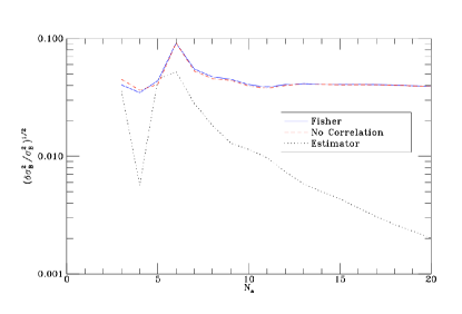
Figure 5: The effect of a 10% gain error on antenna 6, calculated via the three methods listed in the previous figure. The quantity ฮดโ€‹ฯƒB2๐›ฟsuperscriptsubscript๐œŽ๐ต2\delta\sigma_{B}^{2} is the difference in variances of the error estimates with and without the gain error. Noise is set to zero in these calculations.
Refer to caption
Refer to caption
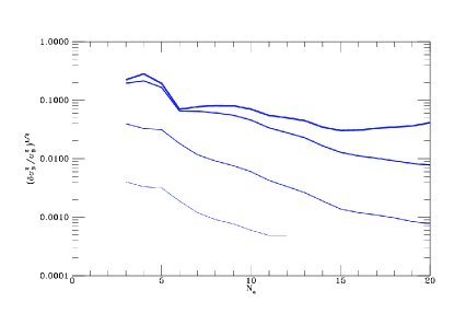
Figure 6: The additional error caused by a gain error in the sixth antenna (left) and a rotation error in the third antenna (right). From bottom to top, the curves correspond to error levels ฯƒp=0.01,0.1,1,10subscript๐œŽ๐‘0.010.1110\sigma_{p}=0.01,0.1,1,10.

IV.2.2 Systematic errors

Suppose that there is a systematic error, such as a gain error or a rotation error, in one of the antennas of our interferometer. As described in Section II.4, we assume that this error can be characterized by an unknown parameter p๐‘p. For instance, in the case of a gain error, the unknown true gain is (1+p)1๐‘(1+p) times the nominal gain, and for a rotation error p๐‘p is the angle by which the polarizers are misaligned. We treat p๐‘p as an additional parameter to be estimated, leading to a 3ร—3333\times 3 augmented Fisher matrix, whose rows and columns correspond to ฮธE,ฮธB,psubscript๐œƒ๐ธsubscript๐œƒ๐ต๐‘\theta_{E},\theta_{B},p. For example, if we introduce a 10% gain error (p=0.1๐‘0.1p=0.1) to the sixth antenna of the array, the Fisher matrix (72) and its inverse (73) are replaced by

Faugsubscript๐นaug\displaystyle F_{\rm aug} =(1794.238.084.233.080.2948.080.294101)absentmatrix1794.238.084.233.080.2948.080.294101\displaystyle=\begin{pmatrix}179&4.23&8.08\\ 4.23&3.08&0.294\\ 8.08&0.294&101\end{pmatrix} (75)
Faugโˆ’1superscriptsubscript๐นaug1\displaystyle F_{\rm aug}^{-1} =(0.00579โˆ’0.00791โˆ’0.000439โˆ’0.007910.33588000โˆ’0.000346โˆ’0.000439โˆ’0.0003460.00993)absentmatrix0.005790.007910.0004390.007910.335880000.0003460.0004390.0003460.00993\displaystyle=\begin{pmatrix}0.00579&-0.00791&-0.000439\\ -0.00791&0.33588000&-0.000346\\ -0.000439&-0.000346&0.00993\end{pmatrix} (76)

We see that the existence of this gain error increases the variance ฯƒB2superscriptsubscript๐œŽ๐ต2\sigma_{B}^{2} for about 0.0036%percent0.00360.0036\%.

Figure 5 shows the effect of a 10% gain error in the sixth antenna, according to the three methods. The quantity plotted is (ฮดโ€‹ฯƒB2/ฯƒB2)1/2superscript๐›ฟsuperscriptsubscript๐œŽ๐ต2superscriptsubscript๐œŽ๐ต212(\delta\sigma_{B}^{2}/\sigma_{B}^{2})^{1/2}, where ฮดโ€‹ฯƒB2=(ฯƒB2)sysโˆ’(ฯƒB2)noโ€‹sys๐›ฟsuperscriptsubscript๐œŽ๐ต2subscriptsuperscriptsubscript๐œŽ๐ต2syssubscriptsuperscriptsubscript๐œŽ๐ต2nosys\delta\sigma_{B}^{2}=(\sigma_{B}^{2})_{\rm sys}-(\sigma_{B}^{2})_{\rm no\ sys} is the difference in the variances of the estimates of B power with and without the systematic error.

IV.3 Gain and rotation errors

Figure 6 shows sample results of the systematic error calculations based on the full Fisher matrix calculation. The left panel shows the additional error induced by a gain error in the sixth antenna as a function of array size Nasubscript๐‘๐‘ŽN_{a}, for four different values of the rms gain error ฯƒpsubscript๐œŽ๐‘\sigma_{p}. The right panel shows the same results for a rotation error in the third antenna. In this case, the error parameter p๐‘p is the angle through which the polarizer has been rotated in radians. In both cases, the noise level is set to 0.0002 ฮผ๐œ‡\muK.

In these sample results, we assumed an error that affected a single antenna, but in a realistic experiment, we would expect all antennas to be affected. The rigorous way to deal with this is to parameterize each of the systematic, build a large augmented Fisher matrix, and calculate ฯƒBsubscript๐œŽ๐ต\sigma_{B} from the resulting matrix. However, it is more convenient if we can treat each systematic error separately and add up the resulting ฯƒBsubscript๐œŽ๐ต\sigma_{B}โ€™s. The validity of this approach, of course, depends on the accuracy of treating the individual errors as independent.

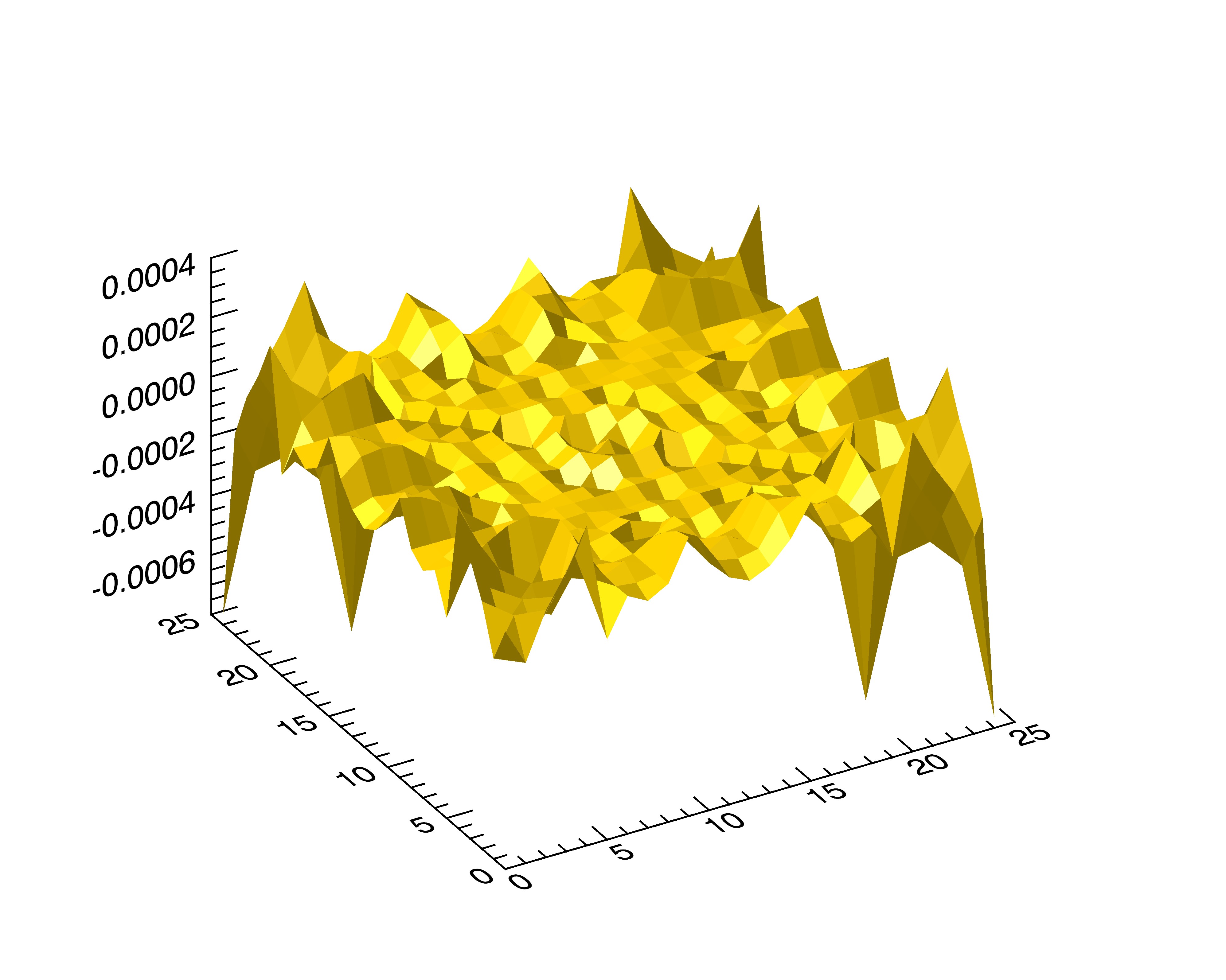
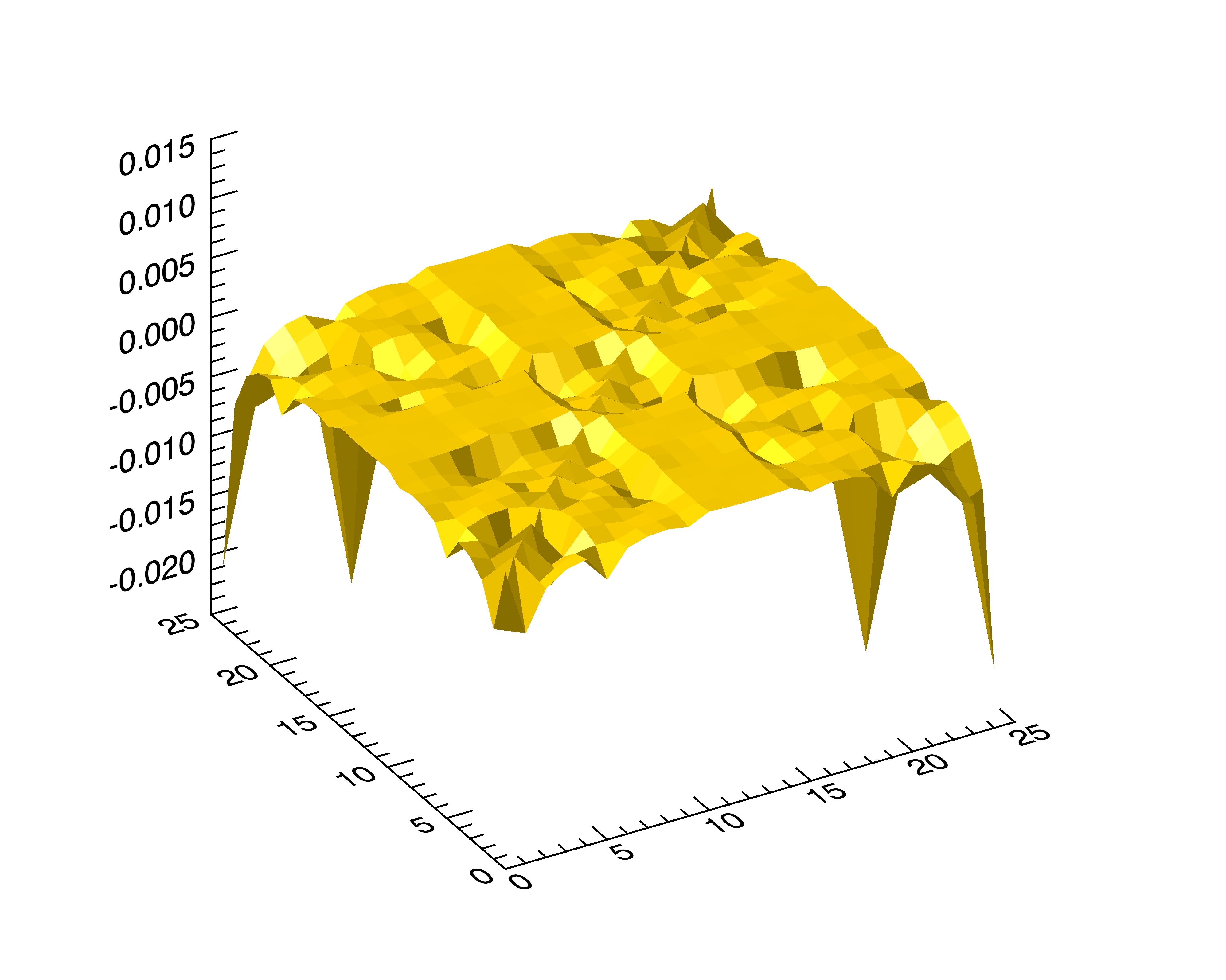
Figure 7 shows the results of tests of this independence assumption. For an array with Na=5subscript๐‘๐‘Ž5N_{a}=5 and n=0.0002โ€‹ฮผ๐‘›0.0002๐œ‡n=0.0002\,\muK, we calculated the effects of a 10% gain error in each of the 25 antennas. We also calculated the effect of simultaneous gain errors in each antenna pair. The quantity plotted is the difference between the simultaneous treatment and the quadrature sum of the individual errors, specifically

ฮ”iโ€‹jโ‰ก(ฮดโ€‹ฯƒB2)iโ€‹jโˆ’((ฮดโ€‹ฯƒB2)i+(ฮดโ€‹ฯƒB2)j)(ฮดโ€‹ฯƒB2)i+(ฮดโ€‹ฯƒB2)j,subscriptฮ”๐‘–๐‘—subscript๐›ฟsuperscriptsubscript๐œŽ๐ต2๐‘–๐‘—subscript๐›ฟsuperscriptsubscript๐œŽ๐ต2๐‘–subscript๐›ฟsuperscriptsubscript๐œŽ๐ต2๐‘—subscript๐›ฟsuperscriptsubscript๐œŽ๐ต2๐‘–subscript๐›ฟsuperscriptsubscript๐œŽ๐ต2๐‘—\Delta_{ij}\equiv{(\delta\sigma_{B}^{2})_{ij}-((\delta\sigma_{B}^{2})_{i}+(\delta\sigma_{B}^{2})_{j})\over(\delta\sigma_{B}^{2})_{i}+(\delta\sigma_{B}^{2})_{j}}, (77)

where i,j๐‘–๐‘—i,j label antennas and ฮดโ€‹ฯƒB2๐›ฟsuperscriptsubscript๐œŽ๐ต2\delta\sigma_{B}^{2} is the additional variance induced by the given error.

The right panel shows the equivalent results for a rotation error of 0.1 rad.

In both cases, the smallness of ฮ”iโ€‹jsubscriptฮ”๐‘–๐‘—\Delta_{ij} indicates that treating the errors as independent is a good approximation, although the case of rotation errors is not as good as that of gain errors.
Refer to caption
Refer to caption
Figure 7: The inaccuracy caused by treating simultaneous errors in two antennas as if they were independent. The horizontal axes are the antennas of a 5ร—5555\times 5 array. The vertical axi is the quantity ฮ”iโ€‹jsubscriptฮ”๐‘–๐‘—\Delta_{ij} of equation (77).

V discussion

We have presented a Fisher-matrix formalism for assessing the errors on power spectrum estimates from intereferometric measurements of CMB polarization, including the effects of systematic errors. This method occupies an intermediate position between crude analytic approximations Bunn (2007) and more accurate but far more computationally intensive end-to-end simulations Karakci etย al. (2013a); Zhang etย al. (2013); Karakci etย al. (2013b). Although detailed simulations are necessary in the end, a fast semianalytic approach such as ours is likely to be useful during the early, exploratory phase of instrument design and optimization.

We have tested our method in a variety of ways, focusing particularly on systematic errors in antenna gain and in the orientation of polarizers of an antenna. Other sources of error can be treated in a similar way. In the absence of systematic errors, our calculations agree with those of simple analytic approximations. The agreement is less good when systematic errors are included (see Fig.ย 5), which is not surprising given the crudeness of the approximations in the analytic method.

Most of our test results involve errors in a single antenna. Assuming different sources of error are independent, one expects the errors to add in quadrature. We verified for gain and rotation errors that this is a good assumption. In any case, it is not difficult to apply our formalism to the treatment of multiple errors simultaneously.

Because our tests were designed to illustrate the formalism, several idealization were made. We considered a single pointing of the instrument, without including sky rotation or mosaicking Bunn and White (2006). In addition, we assumed a single band power was to be estimated in each of the E๐ธE and B๐ตB power spectra. Finally, the errors we considered all involve only E๐ธE-B๐ตB mixing, without contamination from the temperature anisotropy. There is no reason that our method cannot be extended to include these and other effects.

Although we developed the method for interferometric CMB polarimetry, the formalism developed herein can be applied to a variety of experiments. In particular, it would be very interesting to consider application to 21-cm tomography, which similarly involves extraction of small fluctuations signals from interferometric visibilities. Computationally expensive simulations are often done to assess the sensitivity of such instruments (e.g., Zhang etย al. (2015)), but a faster semianalytic approach may be valuable as well.

Acknowledgments

This work was supported by NSF Awards AST-1410133 and AST-0908319, and by a Summer Fellowship from the University of Richmond School of Arts and Sciences.

References

  • Hu (2003) W.ย Hu, Annals of Physics 303, 203 (2003), eprint astro-ph/0210696.
  • Challinor (2013) A.ย Challinor, in IAU Symposium, edited by M.ย G. Burton, X.ย Cui, and N.ย F.ย H. Tothill (2013), vol. 288 of IAU Symposium, pp. 42โ€“52, eprint 1210.6008.
  • Zaldarriaga and Seljak (1997) M.ย Zaldarriaga and U.ย Seljak, Phys.ย Rev.ย D 55, 1830 (1997), eprint astro-ph/9609170.
  • Seljak and Zaldarriaga (1997) U.ย Seljak and M.ย Zaldarriaga, Physical Review Letters 78, 2054 (1997), eprint astro-ph/9609169.
  • Kamionkowski etย al. (1997a) M.ย Kamionkowski, A.ย Kosowsky, and A.ย Stebbins, Physical Review Letters 78, 2058 (1997a), eprint astro-ph/9609132.
  • Kamionkowski etย al. (1997b) M.ย Kamionkowski, A.ย Kosowsky, and A.ย Stebbins, Phys.ย Rev.ย D 55, 7368 (1997b), eprint astro-ph/9611125.
  • Lewis etย al. (2002) A.ย Lewis, A.ย Challinor, and N.ย Turok, Phys.ย Rev.ย D 65, 023505 (2002).
  • Bunn (2002a) E.ย F. Bunn, Phys.ย Rev.ย D 65, 043003 (2002a).
  • Bunn (2002b) E.ย F. Bunn, Phys.ย Rev.ย D 66, 069902(E) (2002b).
  • Bunn etย al. (2003) E.ย F. Bunn, M.ย Zaldarriaga, M.ย Tegmark, and A.ย de Oliveira-Costa, Phys.ย Rev.ย D 67, 023501 (2003).
  • Bunn (2011) E.ย F. Bunn, Phys.ย Rev.ย D 83, 083003 (2011), eprint 1008.0827.
  • Kim (2011) J.ย Kim, Astron. Astrophys. 531, A32 (2011), eprint 1010.2636.
  • Bowyer etย al. (2011) J.ย Bowyer, A.ย H. Jaffe, and D.ย I. Novikov, ArXiv e-prints (2011), eprint 1101.0520.
  • Lewis (2003) A.ย Lewis, Phys.ย Rev.ย D 68, 083509 (2003), eprint astro-ph/0305545.
  • Park and Ng (2004) C.-G. Park and K.-W. Ng, Astrophys.ย J.ย  609, 15 (2004), eprint astro-ph/0304167.
  • Smith (2006a) K.ย M. Smith, Phys.ย Rev.ย D 74, 083002 (2006a), eprint astro-ph/0511629.
  • Smith (2006b) K.ย M. Smith, New Astron.ย Rev. 50, 1025 (2006b), eprint astro-ph/0608662.
  • Smith and Zaldarriaga (2007) K.ย M. Smith and M.ย Zaldarriaga, Phys.ย Rev.ย D 76, 043001 (2007), eprint astro-ph/0610059.
  • Cao and Fang (2009) L.ย Cao and L.-Z. Fang, Astrophys.ย J.ย  706, 1545 (2009), eprint 0910.4697.
  • Zhao and Baskaran (2010) W.ย Zhao and D.ย Baskaran, Phys.ย Rev.ย D 82, 023001 (2010), eprint 1005.1201.
  • Karakci etย al. (2013a) A.ย Karakci, P.ย M. Sutter, L.ย Zhang, E.ย F. Bunn, A.ย Korotkov, P.ย Timbie, G.ย S. Tucker, and B.ย D. Wandelt, Astrophys. J. Supp. 204, 10 (2013a), eprint 1209.2930.
  • Zhang etย al. (2013) L.ย Zhang, A.ย Karakci, P.ย M. Sutter, E.ย F. Bunn, A.ย Korotkov, P.ย Timbie, G.ย S. Tucker, and B.ย D. Wandelt, Astrophys. J. Supp. 206, 24 (2013), eprint 1209.2676.
  • Karakci etย al. (2013b) A.ย Karakci, L.ย Zhang, P.ย M. Sutter, E.ย F. Bunn, A.ย Korotkov, P.ย Timbie, G.ย S. Tucker, and B.ย D. Wandelt, Astrophys. J. Supp. 207, 14 (2013b), eprint 1302.6608.
  • Sutter etย al. (2012) P.ย M. Sutter, B.ย D. Wandelt, and S.ย S. Malu, Astrophys. J. Supp. 202, 9 (2012), eprint 1109.4640.
  • Hu etย al. (2003) W.ย Hu, M.ย M. Hedman, and M.ย Zaldarriaga, Phys.ย Rev.ย D 67, 043004 (2003).
  • Bunn (2007) E.ย F. Bunn, Phys.ย Rev.ย D 75, 083517 (2007), eprint astro-ph/0607312.
  • Readhead etย al. (2004) A.ย C.ย S. Readhead, S.ย T. Myers, T.ย J. Pearson, J.ย L. Sievers, B.ย S. Mason, C.ย R. Contaldi, J.ย R. Bond, R.ย Bustos, P.ย Altamirano, C.ย Achermann, etย al., Science 306, 836 (2004), eprint astro-ph/0409569.
  • Leitch etย al. (2005) E.ย M. Leitch, J.ย M. Kovac, N.ย W. Halverson, J.ย E. Carlstrom, C.ย Pryke, and M.ย W.ย E. Smith, Astrophys.ย J.ย  624, 10 (2005), eprint astro-ph/0409357.
  • Hobson etย al. (1995) M.ย P. Hobson, A.ย N. Lasenby, and M.ย Jones, M.N.R.A.S. 275, 863 (1995).
  • Hobson and Magueijo (1996) M.ย P. Hobson and J.ย Magueijo, M.N.R.A.S. 283, 1133 (1996), eprint astro-ph/9603064.
  • White etย al. (1999) M.ย White, J.ย E. Carlstrom, M.ย Dragovan, and W.ย L. Holzapfel, Astrophys.ย J.ย  514, 12 (1999), eprint astro-ph/9712195.
  • Hobson and Maisinger (2002) M.ย P. Hobson and K.ย Maisinger, M.N.R.A.S. 334, 569 (2002), eprint astro-ph/0201438.
  • Myers etย al. (2003) S.ย T. Myers, C.ย R. Contaldi, J.ย R. Bond, U.-L. Pen, D.ย Pogosyan, S.ย Prunet, J.ย L. Sievers, B.ย S. Mason, T.ย J. Pearson, A.ย C.ย S. Readhead, etย al., Astrophys.ย J.ย  591, 575 (2003), eprint astro-ph/0205385.
  • Bunn and White (2006) E.ย F. Bunn and M.ย White, ArXiv Astrophysics e-prints (2006), eprint astro-ph/0606454.
  • Piat etย al. (2012) M.ย Piat, E.ย Battistelli, A.ย Baรน, D.ย Bennett, L.ย Bergรฉ, J.-P. Bernard, P.ย de Bernardis, M.-A. Bigot-Sazy, G.ย Bordier, A.ย Bounab, etย al., Journal of Low Temperature Physics 167, 872 (2012).
  • Ghribi etย al. (2014) A.ย Ghribi, J.ย Aumont, E.ย S. Battistelli, A.ย Bau, B.ย Bรฉlier, L.ย Bergรฉ, J.-P. Bernard, M.ย Bersanelli, M.-A. Bigot-Sazy, G.ย Bordier, etย al., Journal of Low Temperature Physics 176, 698 (2014), eprint 1307.5701.
  • Pritchard and Loeb (2012) J.ย R. Pritchard and A.ย Loeb, Reports on Progress in Physics 75, 086901 (2012), eprint 1109.6012.
  • Morales and Wyithe (2010) M.ย F. Morales and J.ย S.ย B. Wyithe, Ann.ย Rev.ย Astron.ย Astrophys.ย  48, 127 (2010), eprint 0910.3010.
  • Berger (1993) J.ย O. Berger, Statistical Decision Theory and Bayesian Analysis (Springer, 1993), 2nd ed.
  • Planck Collaboration etย al. (2014) Planck Collaboration, P.ย A.ย R. Ade, N.ย Aghanim, C.ย Armitage-Caplan, M.ย Arnaud, M.ย Ashdown, F.ย Atrio-Barandela, J.ย Aumont, C.ย Baccigalupi, A.ย J. Banday, etย al., Astron. Astrophys. 571, A16 (2014), eprint 1303.5076.
  • Zhang etย al. (2015) L.ย Zhang, E.ย F. Bunn, A.ย Karakci, A.ย Korotkov, P.ย M. Sutter, P.ย T. Timbie, G.ย S. Tucker, and B.ย D. Wandelt, ArXiv e-prints (2015), eprint 1505.04146.

Appendix A The detailed form of the visibility covariance matrix

We assume a Gaussian antenna pattern as in equation (5),

Aโ€‹(๐ซ)=eโˆ’๐ซ2/2โ€‹b2(5),๐ด๐ซsuperscript๐‘’superscript๐ซ22superscript๐‘25\hskip 56.9055ptA(\mathbf{r})=e^{-\mathbf{r}^{2}/{2b^{2}}}\hskip 99.58464pt(\ref{antennaPattern}),

whose Fourier transform is

A~โ€‹(๐ค)=A~โˆ—โ€‹(๐ค)=b22โ€‹ฯ€โ€‹eโˆ’b2โ€‹๐ค2/2,~๐ด๐คsuperscript~๐ด๐คsuperscript๐‘22๐œ‹superscript๐‘’superscript๐‘2superscript๐ค22\tilde{A}(\mathbf{k})=\tilde{A}^{*}(\mathbf{k})=\frac{b^{2}}{2\pi}e^{-b^{2}\mathbf{k}^{2}/2}, (78)

Substituting this into equation (41), we find

โŸจVQโ€‹(๐ฎ1)โ€‹VQโˆ—โ€‹(๐ฎ2)โŸฉdelimited-โŸจโŸฉsubscript๐‘‰๐‘„subscript๐ฎ1superscriptsubscript๐‘‰๐‘„subscript๐ฎ2\displaystyle\qquad\langle V_{Q}(\mathbf{u}_{1})V_{Q}^{*}(\mathbf{u}_{2})\rangle
=(2โ€‹ฯ€)2โ€‹โˆซ[PEโ€‹(๐ค)โ€‹cos2โก(2โ€‹ฯ•)+PBโ€‹(๐ค)โ€‹sin2โก(2โ€‹ฯ•)]absentsuperscript2๐œ‹2delimited-[]subscript๐‘ƒ๐ธ๐คsuperscript22italic-ฯ•subscript๐‘ƒ๐ต๐คsuperscript22italic-ฯ•\displaystyle=(2\pi)^{2}\int{[P_{E}(\mathbf{k})\cos^{2}(2\phi)+P_{B}(\mathbf{k})\sin^{2}(2\phi)]}
A~โˆ—โ€‹(๐ค+2โ€‹ฯ€โ€‹๐ฎ1)โ€‹A~โ€‹(๐ค+2โ€‹ฯ€โ€‹๐ฎ2)โ€‹d2โ€‹๐ค(41)superscript~๐ด๐ค2๐œ‹subscript๐ฎ1~๐ด๐ค2๐œ‹subscript๐ฎ2superscript๐‘‘2๐ค41\displaystyle\qquad\tilde{A}^{*}(\mathbf{k}+2\pi\mathbf{u}_{1})\tilde{A}(\mathbf{k}+2\pi\mathbf{u}_{2})d^{2}\mathbf{k}\hskip 65.44142pt(\ref{vqvq})

Then

โŸจVQโ€‹(๐ฎ1)โ€‹VQโˆ—โ€‹(๐ฎ2)โŸฉdelimited-โŸจโŸฉsubscript๐‘‰๐‘„subscript๐ฎ1superscriptsubscript๐‘‰๐‘„subscript๐ฎ2\displaystyle\qquad\langle V_{Q}(\mathbf{u}_{1})V_{Q}^{*}(\mathbf{u}_{2})\rangle
=b4โ€‹โˆซ[PEโ€‹(๐ค)โ€‹cos2โก(2โ€‹ฯ•)+PBโ€‹(๐ค)โ€‹sin2โก(2โ€‹ฯ•)]absentsuperscript๐‘4delimited-[]subscript๐‘ƒ๐ธ๐คsuperscript22italic-ฯ•subscript๐‘ƒ๐ต๐คsuperscript22italic-ฯ•\displaystyle=b^{4}\int{[P_{E}(\mathbf{k})\cos^{2}(2\phi)+P_{B}(\mathbf{k})\sin^{2}(2\phi)]}
expโก[โˆ’12โ€‹b2โ€‹[(๐ค+2โ€‹ฯ€โ€‹๐ฎ1)2+(๐ค+2โ€‹ฯ€โ€‹๐ฎ2)2]]โ€‹d2โ€‹๐ค12superscript๐‘2delimited-[]superscript๐ค2๐œ‹subscript๐ฎ12superscript๐ค2๐œ‹subscript๐ฎ22superscript๐‘‘2๐ค\displaystyle\qquad\exp\left[-\frac{1}{2}b^{2}\left[(\mathbf{k}+2\pi\mathbf{u}_{1})^{2}+(\mathbf{k}+2\pi\mathbf{u}_{2})^{2}\right]\right]d^{2}\mathbf{k}
=b4โ€‹โˆซ[PEโ€‹(k)โ€‹cos2โก(2โ€‹ฯ•)+PBโ€‹(k)โ€‹sin2โก(2โ€‹ฯ•)]absentsuperscript๐‘4delimited-[]subscript๐‘ƒ๐ธ๐‘˜superscript22italic-ฯ•subscript๐‘ƒ๐ต๐‘˜superscript22italic-ฯ•\displaystyle=b^{4}\int{[P_{E}(k)\cos^{2}(2\phi)+P_{B}(k)\sin^{2}(2\phi)]}
exp[โˆ’b2[2ฯ€2(u12+u22)+k2]โˆ’2ฯ€b2\displaystyle\qquad\exp\big{[}-b^{2}\left[2\pi^{2}(u_{1}^{2}+u_{2}^{2})+k^{2}\right]-2\pi b^{2}
[(u1โ€‹x+u2โ€‹x)kcosฯ•+(u1โ€‹y+u2โ€‹y)ksinฯ•]]kdkdฯ•.\displaystyle\qquad\left[(u_{1x}+u_{2x})k\cos\phi+(u_{1y}+u_{2y})k\sin\phi\right]\big{]}kdkd\phi. (79)

For convenience, we make the following definitions:

S1โ€‹(k)=โˆซ02โ€‹ฯ€cos2โก(2โ€‹ฯ•)subscript๐‘†1๐‘˜superscriptsubscript02๐œ‹superscript22italic-ฯ•\displaystyle S_{1}(k)=\int_{0}^{2\pi}\cos^{2}(2\phi)
expโก[โˆ’2โ€‹ฯ€โ€‹b2โ€‹[(u1โ€‹x+u2โ€‹x)โ€‹kโ€‹cosโกฯ•+(u1โ€‹y+u2โ€‹y)โ€‹kโ€‹sinโกฯ•]]โ€‹dโ€‹ฯ•,2๐œ‹superscript๐‘2delimited-[]subscript๐‘ข1๐‘ฅsubscript๐‘ข2๐‘ฅ๐‘˜italic-ฯ•subscript๐‘ข1๐‘ฆsubscript๐‘ข2๐‘ฆ๐‘˜italic-ฯ•๐‘‘italic-ฯ•\displaystyle\exp\left[-2\pi b^{2}\left[(u_{1x}+u_{2x})k\cos\phi+(u_{1y}+u_{2y})k\sin\phi\right]\right]d\phi, (80)
S2โ€‹(k)=โˆซ02โ€‹ฯ€sin2โก(2โ€‹ฯ•)subscript๐‘†2๐‘˜superscriptsubscript02๐œ‹superscript22italic-ฯ•\displaystyle S_{2}(k)=\int_{0}^{2\pi}\sin^{2}(2\phi)
expโก[โˆ’2โ€‹ฯ€โ€‹b2โ€‹[(u1โ€‹x+u2โ€‹x)โ€‹kโ€‹cosโกฯ•+(u1โ€‹y+u2โ€‹y)โ€‹kโ€‹sinโกฯ•]]โ€‹dโ€‹ฯ•,2๐œ‹superscript๐‘2delimited-[]subscript๐‘ข1๐‘ฅsubscript๐‘ข2๐‘ฅ๐‘˜italic-ฯ•subscript๐‘ข1๐‘ฆsubscript๐‘ข2๐‘ฆ๐‘˜italic-ฯ•๐‘‘italic-ฯ•\displaystyle\exp\left[-2\pi b^{2}\left[(u_{1x}+u_{2x})k\cos\phi+(u_{1y}+u_{2y})k\sin\phi\right]\right]d\phi, (81)
S3โ€‹(k)=โˆซ02โ€‹ฯ€sinโก(4โ€‹ฯ•)subscript๐‘†3๐‘˜superscriptsubscript02๐œ‹4italic-ฯ•\displaystyle S_{3}(k)=\int_{0}^{2\pi}\sin(4\phi)
expโก[โˆ’2โ€‹ฯ€โ€‹b2โ€‹[(u1โ€‹x+u2โ€‹x)โ€‹kโ€‹cosโกฯ•+(u1โ€‹y+u2โ€‹y)โ€‹kโ€‹sinโกฯ•]]โ€‹dโ€‹ฯ•,2๐œ‹superscript๐‘2delimited-[]subscript๐‘ข1๐‘ฅsubscript๐‘ข2๐‘ฅ๐‘˜italic-ฯ•subscript๐‘ข1๐‘ฆsubscript๐‘ข2๐‘ฆ๐‘˜italic-ฯ•๐‘‘italic-ฯ•\displaystyle\exp\left[-2\pi b^{2}\left[(u_{1x}+u_{2x})k\cos\phi+(u_{1y}+u_{2y})k\sin\phi\right]\right]d\phi, (82)

and

qโ€‹(x)=expโก[โˆ’b2โ€‹[2โ€‹ฯ€2โ€‹(u12+u22)+k2]].๐‘ž๐‘ฅsuperscript๐‘2delimited-[]2superscript๐œ‹2superscriptsubscript๐‘ข12superscriptsubscript๐‘ข22superscript๐‘˜2q(x)=\exp\left[-b^{2}[2\pi^{2}(u_{1}^{2}+u_{2}^{2})+k^{2}]\right]. (83)

Then one can check that

โŸจVQโ€‹(๐ฎ1)โ€‹VQโˆ—โ€‹(๐ฎ2)โŸฉdelimited-โŸจโŸฉsubscript๐‘‰๐‘„subscript๐ฎ1superscriptsubscript๐‘‰๐‘„subscript๐ฎ2\displaystyle\langle V_{Q}(\mathbf{u}_{1})V_{Q}^{*}(\mathbf{u}_{2})\rangle =b4โ€‹โˆซ0โˆžPEโ€‹(k)โ€‹qโ€‹(k)โ€‹S1โ€‹(k)โ€‹kโ€‹๐‘‘kabsentsuperscript๐‘4superscriptsubscript0subscript๐‘ƒ๐ธ๐‘˜๐‘ž๐‘˜subscript๐‘†1๐‘˜๐‘˜differential-d๐‘˜\displaystyle=b^{4}\int_{0}^{\infty}P_{E}(k)q(k)S_{1}(k)kdk
+b4โ€‹โˆซ0โˆžPBโ€‹(k)โ€‹qโ€‹(k)โ€‹S2โ€‹(k)โ€‹kโ€‹๐‘‘k.superscript๐‘4superscriptsubscript0subscript๐‘ƒ๐ต๐‘˜๐‘ž๐‘˜subscript๐‘†2๐‘˜๐‘˜differential-d๐‘˜\displaystyle\quad+b^{4}\int_{0}^{\infty}P_{B}(k)q(k)S_{2}(k)kdk. (84)

Similarly, for the U๐‘ˆU-U๐‘ˆU and Q๐‘„Q-U๐‘ˆU covariance matrix elements,

โŸจVUโ€‹(๐ฎ1)โ€‹VUโˆ—โ€‹(๐ฎ2)โŸฉdelimited-โŸจโŸฉsubscript๐‘‰๐‘ˆsubscript๐ฎ1superscriptsubscript๐‘‰๐‘ˆsubscript๐ฎ2\displaystyle\langle V_{U}(\mathbf{u}_{1})V_{U}^{*}(\mathbf{u}_{2})\rangle =b4โ€‹โˆซ0โˆžPBโ€‹(k)โ€‹qโ€‹(k)โ€‹S1โ€‹(k)โ€‹kโ€‹๐‘‘kabsentsuperscript๐‘4superscriptsubscript0subscript๐‘ƒ๐ต๐‘˜๐‘ž๐‘˜subscript๐‘†1๐‘˜๐‘˜differential-d๐‘˜\displaystyle=b^{4}\int_{0}^{\infty}P_{B}(k)q(k)S_{1}(k)kdk
+b4โ€‹โˆซ0โˆžPEโ€‹(k)โ€‹qโ€‹(k)โ€‹S2โ€‹(k)โ€‹kโ€‹๐‘‘k.superscript๐‘4superscriptsubscript0subscript๐‘ƒ๐ธ๐‘˜๐‘ž๐‘˜subscript๐‘†2๐‘˜๐‘˜differential-d๐‘˜\displaystyle\quad+b^{4}\int_{0}^{\infty}P_{E}(k)q(k)S_{2}(k)kdk. (85)
โŸจVQโ€‹(๐ฎ1)โ€‹VUโˆ—โ€‹(๐ฎ2)โŸฉdelimited-โŸจโŸฉsubscript๐‘‰๐‘„subscript๐ฎ1superscriptsubscript๐‘‰๐‘ˆsubscript๐ฎ2\displaystyle\langle V_{Q}(\mathbf{u}_{1})V_{U}^{*}(\mathbf{u}_{2})\rangle =โˆ’12โ€‹b4โ€‹โˆซ0โˆžPEโ€‹(k)โ€‹qโ€‹(k)โ€‹S3โ€‹(k)โ€‹kโ€‹๐‘‘kabsent12superscript๐‘4superscriptsubscript0subscript๐‘ƒ๐ธ๐‘˜๐‘ž๐‘˜subscript๐‘†3๐‘˜๐‘˜differential-d๐‘˜\displaystyle=-\frac{1}{2}b^{4}\int_{0}^{\infty}P_{E}(k)q(k)S_{3}(k)kdk
+12โ€‹b4โ€‹โˆซ0โˆžPBโ€‹(k)โ€‹qโ€‹(k)โ€‹S3โ€‹(k)โ€‹kโ€‹๐‘‘k.12superscript๐‘4superscriptsubscript0subscript๐‘ƒ๐ต๐‘˜๐‘ž๐‘˜subscript๐‘†3๐‘˜๐‘˜differential-d๐‘˜\displaystyle\quad+\frac{1}{2}b^{4}\int_{0}^{\infty}P_{B}(k)q(k)S_{3}(k)kdk. (86)

Equations (A), (A), and (A), combined with equations (A), (A), (A), and (83), are sufficient to present a workable algorithm to calculate the visibility covariance matrix. We now provide the analytic forms of the integrals S1subscript๐‘†1S_{1}, S2subscript๐‘†2S_{2}, and S3subscript๐‘†3S_{3} as the ending of this section. We will take S1subscript๐‘†1S_{1} as an example and directly give S2subscript๐‘†2S_{2} and S3subscript๐‘†3S_{3}.

Let

a๐‘Ž\displaystyle a =(u1โ€‹x+u2โ€‹x)โ€‹k,absentsubscript๐‘ข1๐‘ฅsubscript๐‘ข2๐‘ฅ๐‘˜\displaystyle=(u_{1x}+u_{2x})k, (87)
b๐‘\displaystyle b =(u1โ€‹y+u2โ€‹y)โ€‹k.absentsubscript๐‘ข1๐‘ฆsubscript๐‘ข2๐‘ฆ๐‘˜\displaystyle=(u_{1y}+u_{2y})k. (88)

Then

S1โ€‹(k)=โˆซcos2โก(2โ€‹ฯ•)โ€‹expโก[โˆ’2โ€‹ฯ€โ€‹b2โ€‹(aโ€‹cosโกฯ•+bโ€‹sinโกฯ•)]โ€‹๐‘‘ฯ•.subscript๐‘†1๐‘˜superscript22italic-ฯ•2๐œ‹superscript๐‘2๐‘Žitalic-ฯ•๐‘italic-ฯ•differential-ditalic-ฯ•S_{1}(k)=\int\cos^{2}(2\phi)\exp\left[-2\pi b^{2}(a\cos\phi+b\sin\phi)\right]d\phi. (89)

Now let

t๐‘ก\displaystyle t =arctanโกba,absent๐‘๐‘Ž\displaystyle=\arctan\frac{b}{a}, (90)
ฮธ๐œƒ\displaystyle\theta =ฯ•+t,absentitalic-ฯ•๐‘ก\displaystyle=\phi+t, (91)
l๐‘™\displaystyle l =a2+b2.absentsuperscript๐‘Ž2superscript๐‘2\displaystyle=\sqrt{a^{2}+b^{2}}. (92)

Then

S1โ€‹(k)subscript๐‘†1๐‘˜\displaystyle S_{1}(k) =โˆซcos2โก(2โ€‹ฮธโˆ’2โ€‹t)โ€‹expโก[โˆ’2โ€‹ฯ€โ€‹b2โ€‹lโ€‹sinโกฮธ]โ€‹๐‘‘ฮธabsentsuperscript22๐œƒ2๐‘ก2๐œ‹superscript๐‘2๐‘™๐œƒdifferential-d๐œƒ\displaystyle=\int\cos^{2}(2\theta-2t)\exp\left[-2\pi b^{2}l\sin\theta\right]d\theta
=โˆซcos2โก(2โ€‹ฮธ)โ€‹cos2โก(2โ€‹t)โ€‹expโก(โˆ’2โ€‹ฯ€โ€‹b2โ€‹lโ€‹sinโกฮธ)โ€‹๐‘‘ฮธabsentsuperscript22๐œƒsuperscript22๐‘ก2๐œ‹superscript๐‘2๐‘™๐œƒdifferential-d๐œƒ\displaystyle=\int\cos^{2}(2\theta)\cos^{2}(2t)\exp(-2\pi b^{2}l\sin\theta)d\theta
+โˆซsin2โก(2โ€‹ฮธ)โ€‹sin2โก(2โ€‹t)โ€‹expโก(โˆ’2โ€‹ฯ€โ€‹b2โ€‹lโ€‹sinโกฮธ)โ€‹๐‘‘ฮธ.superscript22๐œƒsuperscript22๐‘ก2๐œ‹superscript๐‘2๐‘™๐œƒdifferential-d๐œƒ\displaystyle+\int\sin^{2}(2\theta)\sin^{2}(2t)\exp(-2\pi b^{2}l\sin\theta)d\theta. (93)

Define

S11โ€‹(k)subscript๐‘†11๐‘˜\displaystyle S_{11}(k) =โˆซcos2โก(2โ€‹ฮธ)โ€‹expโก(โˆ’2โ€‹ฯ€โ€‹b2โ€‹lโ€‹sinโกฮธ)โ€‹๐‘‘ฮธ,absentsuperscript22๐œƒ2๐œ‹superscript๐‘2๐‘™๐œƒdifferential-d๐œƒ\displaystyle=\int\cos^{2}(2\theta)\exp(-2\pi b^{2}l\sin\theta)d\theta, (94)
S12โ€‹(k)subscript๐‘†12๐‘˜\displaystyle S_{12}(k) =โˆซsin2โก(2โ€‹ฮธ)โ€‹expโก(โˆ’2โ€‹ฯ€โ€‹b2โ€‹lโ€‹sinโกฮธ)โ€‹๐‘‘ฮธ.absentsuperscript22๐œƒ2๐œ‹superscript๐‘2๐‘™๐œƒdifferential-d๐œƒ\displaystyle=\int\sin^{2}(2\theta)\exp(-2\pi b^{2}l\sin\theta)d\theta. (95)

Then

S1โ€‹(k)=S11โ€‹(k)โ€‹cos2โก(2โ€‹t)+S12โ€‹(k)โ€‹sin2โก(2โ€‹t).subscript๐‘†1๐‘˜subscript๐‘†11๐‘˜superscript22๐‘กsubscript๐‘†12๐‘˜superscript22๐‘กS_{1}(k)=S_{11}(k)\cos^{2}(2t)+S_{12}(k)\sin^{2}(2t). (96)

The integrals S11subscript๐‘†11S_{11} and S12subscript๐‘†12S_{12} can be written analytically using the modified Bessel function of the first kind Inโ€‹(x)subscript๐ผ๐‘›๐‘ฅI_{n}(x):

S11โ€‹(k)subscript๐‘†11๐‘˜\displaystyle S_{11}(k) =2l3โ€‹ฯ€2โ€‹b6[lฯ€b2(3+l2ฯ€2b4)I0(2lฯ€b2)\displaystyle=\frac{2}{l^{3}\pi^{2}b^{6}}\big{[}l\pi b^{2}(3+l^{2}\pi^{2}b^{4})I_{0}(2l\pi b^{2})
โˆ’(3+2l2ฯ€2b4)I1(2lฯ€b2)],\displaystyle-(3+2l^{2}\pi^{2}b^{4})I_{1}(2l\pi b^{2})\big{]}, (97)

and

S12โ€‹(k)=2l2โ€‹ฯ€โ€‹b4โ€‹[2โ€‹lโ€‹ฯ€โ€‹b2โ€‹I1โ€‹(2โ€‹lโ€‹ฯ€โ€‹b2)โˆ’3โ€‹I2โ€‹(2โ€‹lโ€‹ฯ€โ€‹b2)].subscript๐‘†12๐‘˜2superscript๐‘™2๐œ‹superscript๐‘4delimited-[]2๐‘™๐œ‹superscript๐‘2subscript๐ผ12๐‘™๐œ‹superscript๐‘23subscript๐ผ22๐‘™๐œ‹superscript๐‘2S_{12}(k)=\frac{2}{l^{2}\pi b^{4}}\big{[}2l\pi b^{2}I_{1}(2l\pi b^{2})-3I_{2}(2l\pi b^{2})\big{]}. (98)

We can follow the similar reasoning to calculate S2subscript๐‘†2S_{2} and S3subscript๐‘†3S_{3}. The results are

S2โ€‹(k)=S11โ€‹(k)โ€‹sin2โก(2โ€‹t)+S12โ€‹(k)โ€‹cos2โก(2โ€‹t),subscript๐‘†2๐‘˜subscript๐‘†11๐‘˜superscript22๐‘กsubscript๐‘†12๐‘˜superscript22๐‘กS_{2}(k)=S_{11}(k)\sin^{2}(2t)+S_{12}(k)\cos^{2}(2t), (99)

and

S3โ€‹(k)subscript๐‘†3๐‘˜\displaystyle S_{3}(k) =โˆ’2โ€‹sinโก(4โ€‹t)l3โ€‹ฯ€2โ€‹b6[lฯ€b2(6+l2ฯ€2b4)I0(2lฯ€b2)\displaystyle=-\frac{2\sin(4t)}{l^{3}\pi^{2}b^{6}}\big{[}l\pi b^{2}(6+l^{2}\pi^{2}b^{4})I_{0}(2l\pi b^{2})
โˆ’2(3+2l2ฯ€2b4)I1(2lฯ€b2)].\displaystyle-2(3+2l^{2}\pi^{2}b^{4})I_{1}(2l\pi b^{2})\big{]}. (100)