Operator product expansion coefficients of the 3D Ising model with a trapping potential
Abstract
Recently the operator product expansion coefficients of the 3D Ising model universality class have been calculated by studying via Monte Carlo simulation the two-point functions perturbed from the critical point with a relevant field. We show that this method can be applied also when the perturbation is performed with a relevant field coupled to a non uniform potential acting as a trap. This setting is described by the trap size scaling ansatz, that can be combined with the general framework of the conformal perturbation in order to write down the correlators , and , from which the operator product expansion coefficients can be estimated. We find , in agreement with the results already known in the literature, and , confirming and improving the previous estimate obtained in the uniform perturbation case.
I Introduction
In recent years approaches based on the bootstrap technique rat1 -elsh3 , within the Conformal Field Theory (CFT) framework, allowed to improve the precision on universal numbers needed to characterize the n-point correlation functions, such as scaling dimensions and Operator Product Algebra (OPE) coefficients. In particular new results have been obtained for the 3D Ising model universality class rglioz rrych , whose scaling dimensions were already known with very high precision from Monte Carlo (MC) simulations hasen . However a similar comparison between different methods is still difficult for the OPE coefficients due to the lack of MC results.
In the reference our a method based on the conformal perturbation theory was implemented for calculating the OPE coefficients from off-critical correlators. The method exploits the short distance expansion of the perturbed two-point functions, written as a power series of the Wilson coefficients derivatives and the one-point functions. This procedure was already known gm -cas , but it was never applied to the three dimensional case. In our the practical feasibility of the method was shown and in particular it was used to extract the OPE coefficients of the 3D Ising model, setting the magnetic field as perturbation, and the following results were found: and .
In order to improve the precision of these results, and also to extend this procedure to another kind of perturbation, we consider now the Ising model perturbed from the critical point with a non uniform confining potential coupled to the spin, obtaining for example this Hamiltonian:
| (1) | ||||
| (2) |
Where is the position vector of the site with respect to the central site of the lattice, is the power exponent of the trap and is the typical length. Therefore we have a central symmetry potential growing towards the edges.
The aim of this paper is to show that the conformal perturbation theory can be applied also in presence of a confining potential and that the OPE coefficients of a model, in our case the 3D Ising model, can be obtained by studying the correlation functions modified by the trap.
There are many reasons to motivate this study: the behavior of the critical system in presence of a trap is well described by the trap size scaling (TSS), a framework based on renormalization group arguments that allows to obtain the scaling laws of the observables at the critical point as a function of the trap parameters. The TSS has been successfully tested in many works both for quantum and classical models trap1 -trapn .
Besides the presence of a trap is a common feature of an experimental setup in which the system has to be confined into a limited region. There are experimental studies reproducing this situation for systems in the U(1) universality class trapex1 -trapex3 .
Finally from a purely theoretical point of view it is interesting to combine the trap size scaling ansatz with the perturbations in CFT, aiming to find the corrections to the two-point functions, because it shows the general applicability of the method, even in this case in which the translational symmetry is explicitly broken.
Moreover there could be some advantages, as we will see the TSS ansatz introduces a further external parameter, that in principle could be used to improve the signal of the perturbation terms that have to be calculated in the MC simulations.
II 3D trapped Ising model
II.1 Trap size scaling ansatz
In order to write down the correlation functions of the 3D Ising model with a trapping potential, it is useful to summarize the general framework of the TSS as established in the original reference trap1 .
From the renormalization group framework (RG) we can write the scaling form of the singular part of the free energy density, near the critical point, with the usual notation but keeping into account a further scaling variable given by the trap:
| (3) |
Where we inserted also the space position to stress that now the translational invariance is lost and the observables are point dependent. Iterating the RG transformation as in the standard approach (near the critical point we can assume ), we obtain:
| (4) |
Where we defined , that is the characteristic trap exponent and can be deduced by means of scaling arguments from the corresponding continuum theory. In fact if we consider the potential (2) as a perturbation coupled to the spin relevant field of a generic conformal action, we can write:
| (5) |
If we perform a scale change with parameter , we have , , and for the field , where is the spin scaling dimension. Since they must compensate within the (5), we deduce:
| (6) |
This expression depends only on the dimensionality of the system, the geometry of the confining trap and the universality class of the model.
From the free energy density at the critical point (, ), we can deduce the scaling behavior of the one-point functions of the spin and the energy in the central point of the trap, respectively:
| (7) | |||
| (8) |
Where , are non universal constants and the label zero emphasizes that we are considering only local observables, typically defined in the central point, since in general the mean values are point dependent.
Moreover the correlation length exhibits a scaling law with the trap parameters. Therefore the singularities of the observables at the critical point are smoothed, being the correlation length limited by the trap. However the TSS has a precise and universal scaling behavior determined by the typical length and the exponent . For this reason we expect the TSS can be applied also in our case for the perturbed correlation functions.
II.2 Correlators in the 3D trapped Ising model
We shortly summarize the method already applied in our . The starting point is the OPE wils written for perturbed systems:
| (9) |
where the are a complete set of operators in CFT, the is the expectation value over the action perturbed with a small relevant parameter . The Wilson coefficients can be expanded as a Taylor series with respect to the perturbation parameter in a regular way without infrared divergences, so that the coefficients of the expansion are the derivatives calculated at gm . In particular we note that the OPE coefficients can be extracted from the first correction term of the critical correlator. Hence by calculating via MC simulations the perturbed two-point functions of relevant operators and the one-point functions, whose behavior is well known from the RG framework, the OPE coefficients can be deduced. For further details see the references our -cas . For example for the spin-spin correlator with the magnetic field perturbation we have:
| (10) |
In our case the trap perturbation breaks the translational symmetry, but it still leaves the rotational symmetry due to the shape of the confining potential (2). Hence if we fix one operator in the center of the trap and the other one at radial distance , the (10) is still valid and the fusion rules between fields are the same of the uniform case. Then substituting the one-point functions (7) and (8), we see that the expansion can be written as power series of the scaling variable , that can be deduced also from the (4). So there is perfect analogy with the uniform magnetic field case, provided that the scaling exponent of the trap and the scaling variable of the TSS ansatz are substituted, and we obtain straightforwardly:
| (11) | |||
| (12) | |||
| (13) |
As in the general case, the expansion series for the correlators, taken from the center up to the distance , converges for distances less than about one correlation length. The desired OPE coefficients are included in the leading perturbation term, so that we can extract them knowing the TSS behavior of the one-point functions. Moreover there are two free parameters, and , that can be adjusted to maximize the relevance of the first correction term of the expansion. Our aim is to check the validity of this scenario via MC simulations and to extract the 3D Ising model OPE coefficients.
III Monte Carlo simulation
III.1 Simulation settings
We perform the simulations on a cubic lattice of side with fixed boundary condition. The trap is centered in the middle point of the cube. On the lattice we denote with the spin located at distance from the center upon the axis . Hence we define the following observables: the spin one-point function on the central site , and the energy one-point function in the middle of the lattice, defined as , where is the energy bulk contribution at the critical point, that must be subtracted.
The correlation functions are calculated from the central site of the lattice up to the distance on the central axis, averaging between the six possible directions. Also for correlators involving the energy the constant bulk contribution has to be subtracted. Therefore we have these definitions:
Usually the site energy is obtained by averaging the products with the neighbor spins in all the directions. However now there is no more translational invariance, therefore, except for the central site, the links in different directions have not the same energy. However in our case the trap acts as a perturbation, so that the energy difference between two neighbor sites due to the broken translational symmetry is negligible. We numerically find that this assumption is correct within the precision of our simulations.
The same attention is needed for the spin-energy correlation function, since in principle with the exchanging of the two operators actually we obtain different correlators. However we anticipate that, for the distances and the trap lengths involved in our simulations, we do not observe differences. This confirms the validity of the selected window of perturbation parameters, since in the theory the operators can be exchanged without differences.
The constraints to select the most appropriate trap parameter and the exponent are the same as in the uniform magnetic field case, i.e. having a sufficient large correlation length to sample the correlator and avoiding the finite size effects. After some tests we find that a potential with power is the best choice, in fact with a smaller exponent the correlation length of the system is short while with larger we have to increase too much the size of the lattice to avoid finite size effects. We have checked that a cubic lattice of side is large enough to prevent them within our current precision.
This is a very large lattice in three dimensions, however since all the observables are closely sampled around the central site of the lattice, we can increase the speed of the simulation by using the hierarchical upgrade. This method can be used when the observable is local: instead of doing the Monte Carlo sweep on the whole lattice before sampling the observable, the sweep is performed only on a box around the point of interest. Actually the algorithm works by defining many boxes of increasing side around the central point, and then performing nested cycles of sweeps on every box. The detailed description can be found for example in the reference hasenbox . In this way we can save time and increase the maximum lattice size. Moreover we sample correlators at different distances in different simulations, so that our data are uncorrelated.
We fix the following constants to their known value: the energy bulk contribution and the critical temperature from reference hasen2 , the scaling dimension and from rrych , with whom we have . The uncertainty on these constants is negligible in our data set.
With these settings we find that the optimal range for the trap parameter is for which the correlation length is around 18 lattice spacings. In these simulations we choose a thermalization time of sweeps, with starting configuration of all spins up aligned, and we sample about configurations for each correlation function.
The two-point functions at the critical point have to be normalized to one as in the continuum, since, for example, the spin-spin correlator on lattice is:
Therefore the spin normalization is , and similarly for the energy . From these we can convert all the quantities from lattice to continuum units. For further details see our and cas .
The constants , are also important because they fix the leading order term of the spin-spin and the energy-energy correlators; as we see in the reference our they are the main source of systematic errors on the final estimate of the OPE coefficients. We fix as in our , while for we have refined the result by finite size scaling study of the critical correlator, obtaining .
III.2 Two-point functions
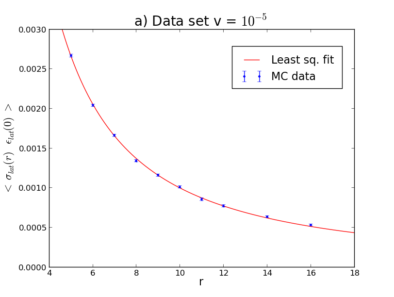
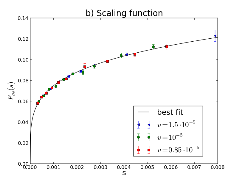
As we learn from the reference our , the spin-energy correlator is the most suitable observable to determine the coefficient since it is zero at the critical point and there is not systematic error. Hence we can fit only the leading order term of (13). The table 1 shows the results of the fit for the values of in the optimal range. The data sets are consistent with the functional form predicted by the TSS ansatz. For comparison we remind the result of the bootstrap approach, for example from rrych , . Our results are in good agreement with this estimate, and thanks to the higher statistics we improve also the previous MC results. Combining all the data series we obtain . In the upper panel of figure 1 the data set for is shown, while in the lower panel all the rescaled data series are plotted in order to show that they are distributed around the expected scaling function .
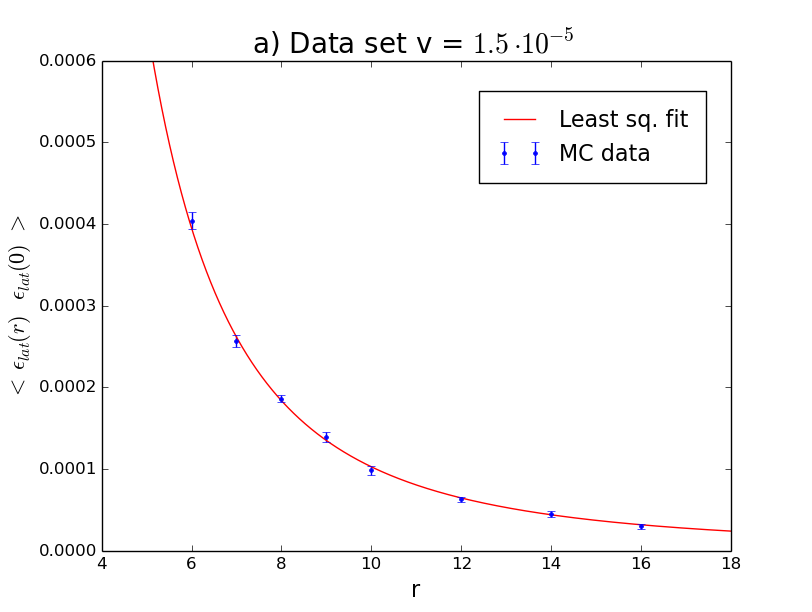
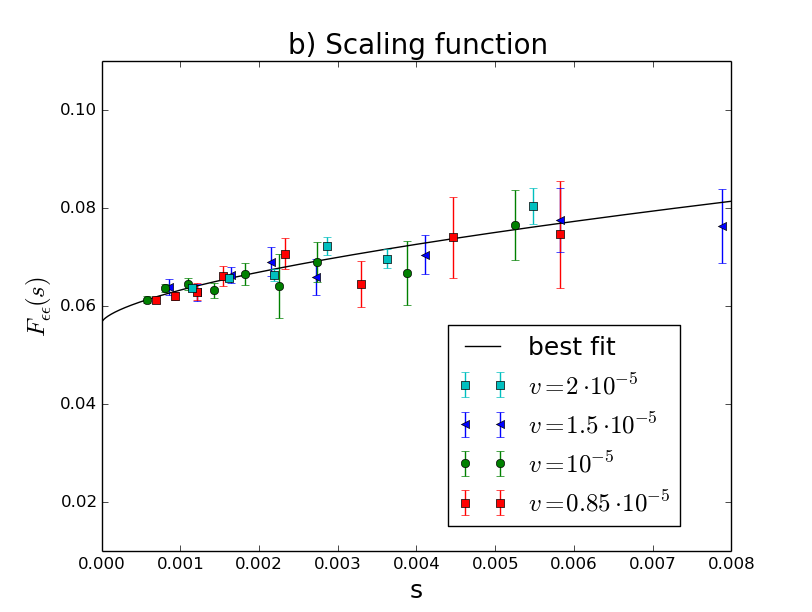
The energy-energy correlator instead is the most interesting to determine the less known coefficient . However this observable has a low signal due to the rapidly decreasing power law, and it is affected by a systematic error due to the critical point term. We adopt the same convention of our denoting the fit statistical error in round brackets and the systematic error in square brackets. The table 2 shows our results, that are fully consistent with the estimate of our , and again we find a good agreement with the expected power law behavior of (12). We quote the final estimate . The figure 2 shows the plot for the data set and the scaling function .
Finally we consider as consistency check the spin-spin correlator, since it is the observable with largest systematic error. Moreover it is affected by short distance corrections, which instead were negligible for the other correlators note . The table 3 shows the results, that are fully consistent with the previous estimates.
| 5 | 16 | 1.054 (6) | 0.7 | |
| 5 | 16 | 1.048 (7) | 1.0 | |
| 5 | 18 | 1.050 (7) | 0.5 |


| 6 | 12 | 1.34(5)[8] | 1.1 | |
| 6 | 16 | 1.32(11)[8] | 0.5 | |
| 6 | 16 | 1.40(10)[10] | 0.6 | |
| 7 | 18 | 1.23(10)[10] | 0.5 |
| 5 | 16 | 1.057 (16) [50] | 1.2 | |
| 5 | 16 | 1.048 (14) [60] | 0.6 | |
| 5 | 18 | 1.061 (21) [70] | 0.9 |
IV Conclusions
We have verified that the method of extracting the OPE coefficients from perturbed correlators works also in presence of a trap: when the confining potential has a very large typical length compared to the distances involved for the correlators, it can be considered as a perturbation and the OPE expansion for the perturbed two-point functions can be wrote following the general prescription.
The trap size scaling ansatz provides the tools to understand the behavior of the one-point functions and the exponents of the power law terms, characterized by the trap exponent . The possibility to combine these tools to describe the perturbed correlators in principle was not ensured, due to the explicit translational symmetry breaking of the potential coupled to the spin operator. Therefore finding the expected OPE coefficients of the 3D Ising model universality class is itself a non trivial result.
Moreover we can extract with a good precision the coefficients and ; unfortunately the latter one, which is very interesting being the most difficult to obtain also with the bootstrap approaches, has higher uncertainty than the former one. However we are confident that this result could be improved with further MC simulations.
Another possibility could be coupling the confining potential to the energy operator, whose trap size scaling has been equally investigated in trap1 . Given our results, there is no reason for which the same kind of study could not be repeated in this other case.
The main limitations to the trap approach are the large size of the lattice generally required (a problem partially recovered by the hierarchical upgrades algorithm), and the fine tuning of the free parameters, the power exponent and the trap length , which requires some preliminary studies to fix the non universal constants and to find the most suitable sampling window. However this drawback is acceptable if it leads to isolate the terms containing the OPE coefficients in the perturbed correlators expansion.
Acknowledgments I would like to thank M. Caselle and N. Magnoli for useful suggestions and the INFN Pisa GRID data center for supporting the numerical simulations.


References
- (1) R. Rattazzi, V. S. Rychkov, E. Tonni and A. Vichi, JHEP 0812 (2008) 031 [arXiv:0807.0004 [hep-th]].
- (2) V. S. Rychkov and A. Vichi, Phys. Rev. D 80 (2009) 045006 [arXiv:0905.2211 [hep-th]].
- (3) R. Rattazzi, S. Rychkov and A. Vichi, Phys. Rev. D 83 (2011) 046011 [arXiv:1009.2725 [hep-th]].
- (4) D. Poland and D. Simmons-Duffin, JHEP 1105 (2011) 017 [arXiv:1009.2087 [hep-th]].
- (5) S. El-Showk, M. F. Paulos, D. Poland, S. Rychkov, D. Simmons-Duffin and A. Vichi, Phys. Rev. D 86 (2012) 025022 [arXiv:1203.6064 [hep-th]].
- (6) D. Pappadopulo, S. Rychkov, J. Espin and R. Rattazzi, Phys. Rev. D 86 (2012) 105043 [arXiv:1208.6449 [hep-th]].
- (7) D. Poland, D. Simmons-Duffin and A. Vichi, JHEP 1205 (2012) 110 [arXiv:1109.5176 [hep-th]].
- (8) S. El-Showk and M. F. Paulos, Phys. Rev. Lett. 111 (2013) 241601 [arXiv:1211.2810 [hep-th]].
- (9) Z. Komargodski and A. Zhiboedov, JHEP 1311 (2013) 140 [arXiv:1212.4103 [hep-th]]
- (10) P. Liendo, L. Rastelli and B. C. van Rees, JHEP 1307 (2013) 113 [arXiv:1210.4258 [hep-th]]
- (11) F. Gliozzi, Phys. Rev. Lett. 111 (2013) 161602 [arXiv:1307.3111 [hep-th]]
- (12) F. Kos, D. Poland and D. Simmons-Duffin, JHEP 1406 (2014) 091 [arXiv:1307.6856 [hep-th]]
- (13) F. Kos, D. Poland and D. Simmons-Duffin, JHEP 1411 (2014) 109 [arXiv:1406.4858 [hep-th]]
- (14) D. Gaiotto, D. Mazac and M. F. Paulos, JHEP 1403 (2014) 100 [arXiv:1310.5078 [hep-th]]
- (15) S. El-Showk, M. Paulos, D. Poland, S. Rychkov, D. Simmons-Duffin and A. Vichi, Phys. Rev. Lett. 112 (2014) 141601 [arXiv:1309.5089 [hep-th]]
- (16) F. Gliozzi and A. Rago, JHEP 1410 (2014) 42 [arXiv:1403.6003 [hep-th]]
- (17) S. El-Showk, M. F. Paulos, D. Poland, S. Rychkov, D. Simmons-Duffin, A. Vichi, J. Stat. Phys. 157 (2014) 869 [arXiv:1403.4545 [hep-th]]
- (18) M. Hasenbusch, Phys. Rev. B 82 (2010) 174433 [arXiv:1004.4486 [cond-mat.stat-mech]]
- (19) M. Caselle, G. Costagliola, N. Magnoli, Phys. Rev. D 91 (2015) 061901 [arXiv:1501.04065 [hep-th]]
- (20) R. Guida and N. Magnoli, Nucl. Phys. B 471 (1996) 361 [arXiv:hep-th/9511209]
- (21) R. Guida, N. Magnoli, Nucl.Phys. B 483 (1997) 563 [arXiv:hep-th/9606072]
- (22) R. Guida, N. Magnoli, Int.J.Mod.Phys. A 13 (1998) 1145 [arXiv:hep-th/9612154]
- (23) M. Caselle, P. Grinza and N. Magnoli, J. Phys. A 34 (2001) 8733 [arXiv:1501.04065 [hep-th]]
- (24) M. Campostrini, E. Vicari, Phys. Rev. Lett. 102, 240601 (2009) [arXiv:0903.5153 [cond-mat.stat-mech]]
- (25) M. Campostrini, E. Vicari, Phys. Rev. A 81 (2010) 023606 [arXiv:0906.2640 [cond-mat.stat-mech]]
- (26) S.L.A. de Queiroz, R.R dos Santos, R.B. Stinchcombe, Phys. Rev. E 81 (2010) 051122 [arXiv:1003.1075 [cond-mat.stat-mech]]
- (27) G. Costagliola, E. Vicari, J. Stat. Mech. L08001 (2011) [arXiv:1107.0815 [cond-mat.stat-mech]]
- (28) G. Ceccarelli, C. Torrero, E. Vicari, Phys. Rev. B 87 (2013) 024513 [arXiv:1211.6224 [cond-mat.stat-mech]]
- (29) G. Ceccarelli, J. Nespolo, Phys. Rev. B 89 (2014) 054504 [arXiv:1312.1235 [cond-mat.quant-gas]]
- (30) F.M. Gasparini, M.O. Kimball, K.P. Mooney, M. Diaz-Avilla, Rev. Mod. Phys. 80, 1009 (2008)
- (31) I. Bloch, J. Dalibarad, W. Zwerger, Rev. Mod. Phys. 80, 885 (2008)
- (32) T. Donner, S. Ritter, T. Bourdel, A. Ottl, M. Kohl, T. Esslinger, Science 315, 1556 (2007) [arXiv:0704.1439 [cond-mat.stat-mech]]
- (33) K. G. Wilson, Phys. Rev. 179 (1969) 1499
- (34) M. Caselle, M. Hasenbusch, M. Panero, JHEP 01 (2003) 057 [arXiv:hep-lat/0211012]
- (35) M. Hasenbusch, Phys. Rev. B 85 (2012) 174421 [arXiv:1202.6206 [cond-mat.stat-mech]]
- (36) We fit the spin-spin correlator with , with and as free parameters. The last term takes into account the short distance corrections induced by the next to the leading order term of the correlator at the critical point on the lattice. This anstaz is sufficient to fit the correlator as reported in table 3.