Jet-vetoed Higgs cross section in gluon fusion at N3LO+NNLL with small- resummation
Abstract
We present new results for the jet-veto efficiency and zero-jet cross section in Higgs production through gluon fusion. We incorporate the N3LO corrections to the total cross section, the NNLO corrections to the 1-jet rate, NNLL resummation for the jet and LL resummation for the jet radius dependence. Our results include known finite-mass corrections and are obtained using the jet-veto efficiency method, updated relative to earlier work to take into account what has been learnt from the new precision calculations that we include. For 13 TeV collisions and using our default choice for the renormalisation and factorisation scales, , the matched prediction for the jet-veto efficiency increases the pure N3LO prediction by about 2% and the two have comparable uncertainties. Relative to NNLO+NNLL results, the new prediction is 2% smaller and the uncertainty reduces from more than 10% to less than 5%. Results are also presented for the central scale .
1 Introduction
Since the announcement of the discovery of the Higgs boson Aad:2012tfa ; Chatrchyan:2012xdj , a dynamic research programme has come into place to measure and constrain its properties. The precision of the measurements is already such that the interpretation of data is sometimes limited by theoretical uncertainties (see e.g. Refs. ATLAS:2014aga ; Chatrchyan:2013iaa ). Experimental errors will decrease in Run II, because of the higher luminosity and of the higher energy. Experimental analyses will also benefit from the experience gained in Run I, which will result in optimised Higgs analyses already from the early stages of Run II.
The dominant Higgs-production mode at the LHC is gluon-gluon fusion. The most fundamental quantity is the total Higgs production cross-section, which allows one to compute the total number of Higgs bosons produced at the LHC for a given energy and luminosity. In some Higgs boson decay modes (most notably and ), it is standard to perform different analyses depending on the number of accompanying jets. This is because different jet multiplicities have different dominant backgrounds. Of particular importance for the decay is the zero-jet case, where the dominant top-quark decay background is dramatically reduced. For precision studies it is important to predict accurately the fraction of signal events that survive the zero-jet constraint, and to assess the associated theory uncertainty. Jet-veto transverse momentum thresholds used by ATLAS and CMS are relatively soft ( GeV), hence QCD real radiation is severely constrained by the cut and the imbalance between virtual and real corrections results in logarithms of the form that should be resummed to all orders in the coupling constant. This resummation has been carried out to next-to-next-to-leading logarithmic accuracy (NNLL, i.e. including all terms with in the logarithm of the cross section) and matched to next-to-next-to-leading order (NNLO) in Refs. Banfi:2012jm ; Stewart:2013faa ; Becher:2013xia (some of the calculations also included partial N3LL contributions). At this order one finds that the effect of the resummation is to shift central predictions only moderately, and to reduce somewhat the theoretical uncertainties. Yet, the residual theoretical uncertainty remains sizeable, roughly Banfi:2012jm , and the impact of higher-order effects could therefore be significant.
Since the first NNLO+NNLL predictions for the jet-veto, three important theoretical advances happened: firstly, the N3LO calculation of the total gluon-fusion cross section Anastasiou:2015ema ; secondly the calculation of the NNLO corrections to the Higgs plus one-jet cross-section Boughezal:2015dra ; Boughezal:2015aha ; Caola:2015wna ; and finally the LL resummation of logarithms of the jet-radius Dasgupta:2014yra . Given these recent advances, we are now in a position to improve on the previous prediction by extending the matching of the jet-veto cross-section to N3LO+NNLL+LLR. In order to perform the matching and to estimate the uncertainties one needs to extend the matching schemes introduced in Ref. Banfi:2012jm to one order higher. In doing so, we will also revisit the formulation of the “jet-veto efficiency” (JVE) approach that was introduced in Ref. Banfi:2012yh .
For accurate predictions it is also important to investigate the impact of finite quark masses, a subject extensively discussed in the literature. Finite quark-mass effects are known exactly only up to NLO Spira:1995rr ; Spira:1997dg ; Harlander:2005rq ; Anastasiou:2006hc ; Aglietti:2006tp ; Bonciani:2007ex . The impact of top quark effects on the leading jet’s transverse momentum at NLO has been studied through a expansion Neumann:2014nha . Different prescriptions have been proposed to include top and bottom effects in analytic resummations Mantler:2012bj ; Grazzini:2013mca ; Banfi:2013eda as well as parton-shower simulations, e.g. in (N)NLO+PS generators Bagnaschi:2011tu ; Bagnaschi:2015qta ; Hamilton:2015nsa . Here, we include exact mass effects up to NNLL+NLO and study the impact of the resummation scale associated with the bottom and top-bottom-interference contributions. Mass effects at NNLO and N3LO are currently unknown, so we use the large- limit (without any rescaling) at these orders.
This paper is organised as follows. In Sec. 2.1 we recall the Jet Veto Efficiency (JVE) method, and we give a new prescription for the uncertainty estimate. This differs from the one given in ref. Banfi:2012jm , and we believe is more appropriate now that the Higgs total production and Higgs plus one-jet cross sections are known respectively known through N3LO and NNLO. In the rest of Sec. 2, we introduce the various ingredients of the calculation, and we discuss how they are combined together. In Sec. 3 we present our new results at 13 TeV centre-of-mass energy, while Sec. 4 contains our conclusions. In Appendix A we further motivate the introduction of the new JVE uncertainty prescription. In Appendix B we compare our final predictions obtained with central scale to predictions obtained with central scale . Finally, in Appendix C we give some technical details about the small- resummation.
2 Outline of the formalism
2.1 Updated jet-veto efficiency method at fixed order
The core element of our estimate of uncertainty in the jet-vetoed cross section is the JVE method Banfi:2013eda . The premise of the method is that the zero-jet cross section is given by the product of the total cross section and jet-veto efficiency and that the uncertainties in the two quantities are largely uncorrelated. The argument that motivates this working assumption is that, at small , uncertainties in the efficiency are due to non-cancellation of real and virtual contributions, while those in the total cross section are connected with the large -factor that is observed in going from leading order to higher orders.
The JVE method can be applied both at fixed order and with resummation.111In this respect it differs from the Stewart-Tackmann method Stewart:2011cf , which has so far been applied only to fixed-order calculations. An alternative way to estimate the theoretical uncertainties in the resummed case was proposed in Stewart:2013faa . It is useful to first extract the jet-veto efficiency from the total Higgs cross section and the cross section for Higgs production with a jet veto (i.e. without any jets with ). We define the expansion of the total cross section and of the jet-veto cross-section up to perturbative order as
| (1) |
Furthermore we use to denote (minus) the cross section to have at least one jet above a scale . Its order component is given by
| (2) |
This is related to via
| (3) |
From the above equations it is evident that one can obtain at a given order in by combining the inclusive cross-section and the jet cross-section, both computed at the same order in . Recently the coefficient was computed both for Anastasiou:2015ema and for Boughezal:2015dra ; Boughezal:2015aha ; Caola:2015wna .
The most obvious definition for the jet-veto efficiency is to write it as a ratio using the highest order available in each case. We call this prescription “” and at N3LO it reads
| (4a) | |||
| In earlier work Banfi:2012yh ; Banfi:2012jm , it had been argued that in order to estimate perturbative uncertainties, one should explore all possible ways of writing the series for that retain the desired perturbative accuracy. For example at N3LO one can introduce scheme , as | |||
| (4b) | |||
which is equivalent to scheme up to corrections. Three further schemes are possible at N3LO, where one progressively expands in the denominator while ensuring the correctness of the full expression at N3LO (see Appendix A). This in effect corresponds to using the degree of convergence for each and every one of the previous orders as an input to determining the possible size of unknown N4LO corrections. In the case at hand, however, the early terms of the series show extremely poor convergence, especially at higher energies and when including quark-mass effects. As a result, taking an envelope of all possible schemes leads to uncertainty estimates that grow very large, and contrast with the good convergence observed in practice for the last known order of both the numerator and the denominator. A careful study of this question, summarised in Appendix A, has led us to conclude that it is more appropriate to limit oneself to schemes that give sensitivity to the convergence of just the last order of the perturbative series. This implies that we should take just the two schemes and defined in (4).222When the prescription of Refs. Banfi:2012yh ; Banfi:2012jm was originally introduced, only NNLO results were available. Their last order displayed still rather poor convergence, which justified a more conservative approach.
Specifically, to estimate our uncertainty for a fixed-order prediction, we will take the envelope of scheme with a 7-point scale variation around a central scale ( with ), together with scheme evaluated at . The justification for not having scale variations in scheme is that to include them might effectively correspond to double counting, i.e. summing two sources of uncertainty that may at some level have shared origins.
In the results that follow (unless otherwise specified) we will consider proton–proton collisions, with anti- jets Cacciari:2008gp as implemented in FastJet v. 3.1.2 Cacciari:2011ma , and use NNPDF2.3 parton distribution functions (PDFs) at NNLO Ball:2012cx , accessed through LHAPDF6 Buckley:2014ana , with a strong coupling at the -boson mass of . We choose as the default renormalisation and factorisation scale. No rapidity cuts are applied to the jets.
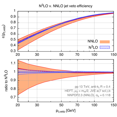
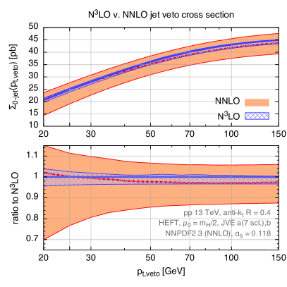
A comparison of NNLO and N3LO results with this prescription, in the effective theory with a large top mass and no bottom mass, is shown in Fig. 1, for both the jet-veto efficiency (left) and the jet-veto cross section (right). One observes a very considerable decrease in the uncertainties in going from NNLO to N3LO with only a modest change in the central values, associated with a small increase in the total cross section from the N3LO corrections Anastasiou:2015ema and a slight decrease in the low- efficiency associated with an increase in the 1-jet cross section at NNLO Boughezal:2015dra ; Boughezal:2015aha ; Caola:2015wna .
2.2 Resummation
Next let us recall the structure of the NNLL resummed jet-veto cross section Banfi:2012jm ,
| (5) |
where we have split the factors involving the parton luminosities into two terms and , which start at order and respectively:
| (6) | ||||
| (7) |
Here is the squared Born matrix element for the partonic scattering channel , is the logarithm we resum, where typically we choose the resummation scale of the order of . is a hard NLO correction, is a NLO coefficient function and is the parton distribution function for flavour at factorisation scale . The strong coupling is always understood to be evaluated at a hard scale , , and the factorisation scale is also to be chosen of the order of . The functions encode the bulk of the LL, NLL and NNLL resummation (for respectively). The and functions, as well as the and coefficients all depend on the choice of . The quantities and Banfi:2012yh account for the NNLL dependence of the result on the jet definition and are further discussed below in section 2.4. Explicit expressions for the above terms are to be found in the supplementary material of Ref. Banfi:2012jm , and a number of the elements are closely related to those derived for resummation Bozzi:2005wk ; Becher:2010tm .
2.3 Matching
To put together the fixed-order and resummed results, we use matching schemes that extend those presented in Ref. Banfi:2012jm to one order higher. We refer the reader to that publication for a detailed explanation of the matching procedure. The matching schemes essentially correspond to the two schemes for the fixed-order efficiency given in Eqs. (4).
To understand our prescriptions for matching, it is first instructive to rewrite the fixed-order schemes for jet-veto efficiencies as ratios of two cross sections:
| (8) |
where admits a different perturbative expansion for each scheme . Specifically, each of the two fixed-order schemes of Eq. (4) can be obtained by combining Eq. (8) with one of the following prescriptions for :
| (9a) | ||||
| (9b) | ||||
Scheme is the exact expansion for and it trivially gives . For scheme , observe that it is simply obtained by multiplying by .333 One could instead arrange for each of the to have the property that it tends to for , however this would complicate the expressions without bringing any actual change in the final results for the jet veto efficiency and cross section.
A further standard element that we need is a modification of the resummation so that its effect switches off for . We do this by replacing , defined as
| (10) |
The choice of is somewhat arbitrary and as in earlier work Banfi:2012yh we take a fairly large value, , to reduce the residual contribution from resummation at high .
For the matched cross-sections we obtain the following results:
| (11a) | ||||
| (11b) | ||||
In the above expressions, denotes the contribution to the NNLL resummed result. The resummed cross section and its expansion are defined in terms of the modified logarithms as defined in Eq. (10). We have also introduced . This quantity admits a perturbative expansion in powers of , starting at order . We denote this expansion as . Note that does not actually depend on . Note also that, as for the fixed-order schemes, the normalisation at is different for each matching scheme, in particular with for . Using Eq. (8), one always recovers the correct normalisation for .
Since the matching schemes above are multiplicative, for small , any finite remainder in the square brackets is multiplied by a Sudakov form factor, ensuring that the cross section and efficiency vanish in the limit , since vanishes in this limit.444Note that this behaviour of can be altered when including the small- resummation. This only happens for rather small values, and it is therefore not present for phenomenologically relevant values of the jet radius.

For matched results, in addition to varying and for scheme and keeping a central choice for scheme (as done in the fixed-order calculations), we also vary in scheme around its default choice of . However, in this work we change our convention for the range of variation relative to earlier studies by some of us Banfi:2012yh ; Banfi:2012jm , which had . We instead choose the range of that had been originally proposed when variation was first introduced Dasgupta:2002dc ; Jones:2003yv . The motivation for returning to this earlier, narrower range comes from the observation of the uncertainties at NNLO+NNLL: with the wider range, the NNLO+NNLL uncertainties come out as unduly large relative the actual changes observed when including N3LO corrections. Moreover, the old variation range gives rise to overly large uncertainties in the tail of the leading jet’s transverse momentum differential spectrum. For a more detailed discussion of this we refer the reader to Appendix A.
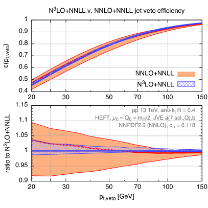
Fig. 2 shows the impact of matching the NNLL resummed results with the N3LO result, compared to NNLO+NNLL results (left) and to pure N3LO results (right). In the left-hand plot, one sees a clear reduction in uncertainties in going from NNLO+NNLL to N3LO+NNLL, as expected given the impact of the N3LO results shown in Fig. 1. While the NNLO+NNLL results had a substantially smaller uncertainty band than pure NNLO, once one includes one additional order in , resummation brings essentially no further reduction, as is visible in the right-hand plot. It does, however, induce a small shift in the central value (and uncertainty band), whose magnitude is slightly smaller than the uncertainty itself.
2.4 Jet-radius dependence and small- effects
Two terms in Eq. (5) are connected with the choice of jet definition and in particular depend on the jet radius . accounts for clustering of independent soft emissions and for commonly used values of is given by Banfi:2012yh ; Banfi:2012jm
| (12) |
Banfi:2012yh comes from the correlated part of the matrix element for the emission of two soft partons. For our purposes it is useful to further split it into two parts,
| (13) |
where the coefficient of the logarithm of is
| (14) |
while the finite (regular) remainder is
| (15) |
This was originally derived including terms up to in Ref. Banfi:2012yh with a numerically-determined constant term, while an analytic form for the constant term and an expansion up to order were given in Ref. Becher:2013xia .
Ref. Tackmann:2012bt advocated resummation of the terms enhanced by powers of . Ref. Dasgupta:2014yra showed that LL small- terms could be incorporated into the jet-veto cross section by replacing with
| (16) |
where (denoted in Ref. Dasgupta:2014yra ) is the LLR resummed result for the first logarithmic moment of the momentum fraction carried by the hardest small- jet resulting from the fragmentation of a gluon. A detailed, partially parametrised, expression for is given in Eq. (C), with tabulated coefficients for in table 7 (the second order coefficient was also calculated in Ref. Alioli:2013hba ). The quantity is an integral of the coupling over scales related to the allowed emission angles, defined specifically as
| (17) |
The nominally free parameter can be understood as a resummation scale for the LLR resummation, or, more physically, the largest allowed emission angle. By default we will take and vary it in the range .
In practice, in Eq. (16) we will make the replacements
| (18a) | ||||
| (18b) | ||||
where , . One sees explicitly from Eq. (18b) that logarithms of (in ) and are being treated on the same footing, i.e. one is including all terms for any and . The expression includes just the logarithms needed to obtain joint NNLL+LLR resummation, without terms that are subleading in this hierarchy (except for those explicitly included as part of a NNLL resummation).555This “minimal” prescription is standard in resummations, however in the limit of sufficiently small and small we have observed certain artefacts that, as far as we understand, can only be cured by including subleading terms. Furthermore, inspecting the formulae, one immediately sees that the combination of small- and small- resummation may cause difficulties, since the smallest physical scale in the problem is now , which for sufficiently small can approach non-perturbative values even when . For commonly-used values of the jet radius and the resummed cross section does not feature this issue, which is irrelevant for the phenomenology shown here. Hence we leave the further study of this question to future work. We thank especially Mrinal Dasgupta for collaboration on this and related aspects.
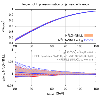
The impact of the small- resummation is shown in Fig. 3, where one sees that it increases the central value of the efficiency by about at , with a slight increase also in the size of the uncertainty band. While it makes sense to include the LLR resummation with a view to providing the most complete prediction possible, for current phenomenological choices of it does not bring a large effect.666Ref. Alioli:2013hba , using a second order calculation of , had also found small- effects that were small.
2.5 Quark-mass corrections
So far we have considered Higgs production in the heavy-top approximation. In this section we study the corrections due to finite top and bottom masses in the loop. Following the procedure of Ref. Banfi:2013eda , the effect of heavy-quark masses at NNLL amounts to simply replacing both the Born squared matrix element and the corresponding one-loop virtual correction with the ones accounting for the correct quark-masses dependence (cf. section 4.1 of ref. Banfi:2013eda ).
We match the NNLL prediction so defined to the N3LO fixed-order cross section where we use the exact mass dependence up to NLO, while keeping the heavy-top approximation for both NNLO and N3LO corrections. We use this as our default prescription for the results presented below. Moreover, we allow for different resummation scales for top and bottom-induced effects. Therefore, we associate to bottom-induced effects (mainly top-bottom interference) an additional resummation scale . The matched cross section, including quark-mass effects then reads
| (19) |
We set to , and vary it as described in section 2.3 () to estimate the associated uncertainty. As far as is concerned, one could either set in the jet-veto efficiency (as done in ref. Banfi:2013eda ) or set it to small scales of the order of , as advocated in Ref. Grazzini:2013mca . As shown in Banfi:2013eda , if the resummation is matched to (at least) NNLO, the impact of changing is very moderate. We show this feature in the left plot of Figure 4 where we compare the jet-veto efficiency obtained with a central to the one obtained with . In order to be more conservative in our test, we vary by a factor of two in either direction in the prediction obtained with , while varying it in the nominal range in the latter case.
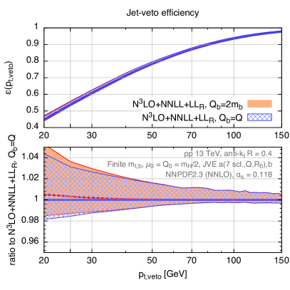
To this order, the difference between the two prescriptions is minimal. We therefore decide to set as our central resummation scales and vary them in a correlated way by a factor 3/2 up and down. With this choice the first and third term in the r.h.s. of Eq. (19) cancel exactly.
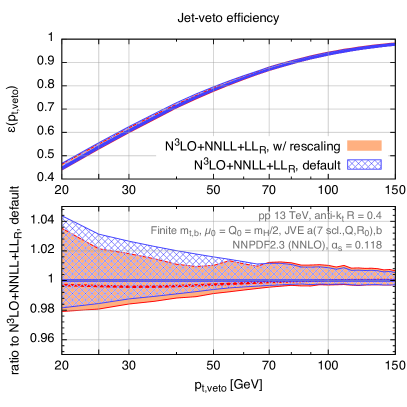
In the context of top-mass corrections only, we note that one could alternatively rescale the NNLO and N3LO corrections by the ratio of the Born cross section with exact top-mass dependence to the corresponding heavy-top result. This rescaling is well justified in the limit of emissions with a transverse momentum much smaller than the top mass. In this region of the spectrum, the corrections to the heavy-top approximation amount to a constant shift up to moderately large . This is indeed the region that contributes the most to the total cross section, even more so when a jet veto is applied. However, it is well known that this is not the case for bottom-quark effects since the region where emissions are softer than the bottom mass is strongly Sudakov-suppressed. This is reflected in the non-trivial shape distortion of the spectrum at normal values Bagnaschi:2011tu ; Grazzini:2013mca ; Banfi:2013eda . Hence, in the small region the above rescaling does not provide a reliable assessment of finite-mass effects.
While it is beyond the scope of this article to give a precise assessment of higher-order mass effects, one can get a rough estimate of their possible impact by comparing our default prescription to the one where one rescales both NNLO and N3LO corrections as discussed above to include finite top-mass effects. We show this in the right-hand plot of Figure 4. We observe very moderate effects of the rescaling down to GeV. This statement is clearly not conclusive, and a more careful study is necessary. Eventually, the issues related to quark-mass effects can only be fixed once a NNLO calculation of mass-effects will be available.
3 N3LO+NNLL+LLR cross section and 0-jet efficiency at 13 TeV
In this section we report our best predictions for the jet-veto efficiency and cross section at the LHC. The various ingredients that we use were discussed in the previous section, but for ease of reference we summarise them here:
-
•
The total N3LO cross section for Higgs production in gluon fusion Anastasiou:2015ema , obtained in the heavy-top limit.777The Wilson coefficient is expanded out consistently both in the computation of the total and the inclusive one jet cross section.
-
•
The inclusive one-jet cross section at NNLO taken from the code of Ref. Caola:2015wna , in the heavy-top limit. In this computation the channel is included only up to NLO, and missing NNLO effects are estimated to be well below scale variation uncertainties Boughezal:2015aha .
-
•
Exact top- and bottom-mass effects up to NLO in the jet-veto efficiency and cross section Spira:1995rr . Beyond NLO, we use the heavy-top result, as explained in section 2.5.
-
•
Large logarithms resummed to NNLL accuracy following the procedure of Banfi:2012jm , with the treatment of quark-mass effects as described in ref. Banfi:2013eda .
-
•
Logarithms of the jet radius resummed to LL accuracy, following the approach of ref. Dasgupta:2014yra .
We consider 13 TeV LHC collisions with a Higgs-boson mass of GeV, compatible with the current experimental measurement Aad:2015zhl . For the top and bottom pole quark masses, we use GeV and GeV. Jets are defined using the anti- algorithm Cacciari:2008gp , as implemented in FastJet v3.1.2 Cacciari:2011ma , with radius parameter , and perform the momentum recombination in the standard scheme (i.e. summing the four-momenta of the pseudo-particles). We use NNPDF 2.3 parton distribution functions at NNLO with (NNPDF23_nnlo_as_0118) Ball:2012cx .888Note that we use a five-flavour evolution for the running coupling as implemented in Hoppet Salam:2008qg , while NNPDF23_nnlo_as_0118 Ball:2012cx uses a six-flavour scheme. This leads to small differences above the top threshold, which are however numerically irrelevant for our study. In our central prediction for the jet-veto efficiency we set renormalisation and factorisation scales to . The resummation scales are set to ,999 applies when including top-bottom interference and bottom contributions, which we do by default here. As shown in section 2.5, switching to the alternative choice makes less than difference. and we use matching scheme (11) as default. In this analysis, we do not include electro-weak corrections Actis:2008ug ; Anastasiou:2008tj ; Keung:2009bs .
To determine the perturbative uncertainties for the jet-veto efficiency we follow the procedure described in section 2.3 and which we summarise here. We vary , by a factor of 2 in either direction, requiring . Maintaining central values, we also vary in the range . As far as the small- effects are concerned, we choose the default value for initial radius for the evolution to be ,101010Note that it acts as a resummation scale for the resummation of logarithms of the jet radius. The initial radius for the small- evolution differs from the jet radius used in the definition of jets, which is . and vary it conservatively by a factor of two in either direction. Finally, keeping all scales at their respective central values, we replace the default matching scheme (11) with scheme (11b). The final uncertainty band is obtained as the envelope of all the above variations. We do not consider here the uncertainties associated with the parton distributions (which mostly affect the cross section, but not the jet veto efficiency), the value of the strong coupling or the impact of finite quark masses on terms beyond NLO (which was discussed in section 2.5).
We report the numerical values for our input total and one-jet cross section in Table 1, with and without mass effects up to , with uncertainties obtained through scale variation and using always NNLO PDFs and .
| LHC 13 TeV [pb] | ||||||
|---|---|---|---|---|---|---|
| EFT | ||||||
| -only | ||||||
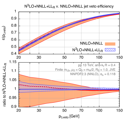
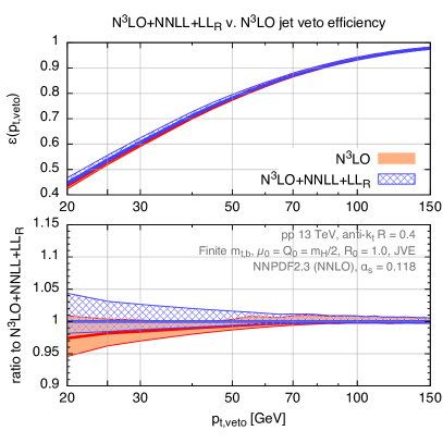
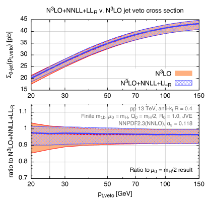
Figure 5 (left) shows the comparison between our best prediction for the jet-veto efficiency (N3LO+NNLL+LLR) and the previous NNLO+NNLL accurate prediction, both including mass effects. We see that the impact of the N3LO correction on the central value is of the order of 2% at relevant jet-veto scales. The uncertainty band is significantly reduced when the N3LO corrections are included, going from about 10% at NNLO down to a few percent at N3LO. Figure 5 (right) shows the comparison between the N3LO+NNLL +LLR prediction and the pure N3LO result. We observe a shift of the central value of the order of 2% for when the resummation is turned on. In that same region, the uncertainty associated with the N3LO prediction is at the 2% level, comparable with that of the N3LO+NNLL +LLR prediction. The fact that resummation effects are of the same order as the uncertainties of the fixed order calculation suggests that the latter might be accidentally small. This situation is peculiar to our central renormalisation and factorisation scale choice, , and does not occur at, for instance, (see Appendix B for details).
The zero-jet cross section is obtained as , and the inclusive one-jet cross section is obtained as . The associated uncertainties are obtained by combining in quadrature the uncertainty on the efficiency obtained as explained above and that on the total cross section, for which we use plain scales variations. The corresponding results are shown in fig. 6. For this scale choice, we observe that the effect of including higher-order corrections in the zero-jet cross section is quite moderate at relevant scales. This is because the small factor in the total cross section compensates for the suppression in the jet-veto efficiency. The corresponding theoretical uncertainty is reduced by more than a factor of two.
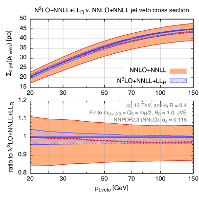
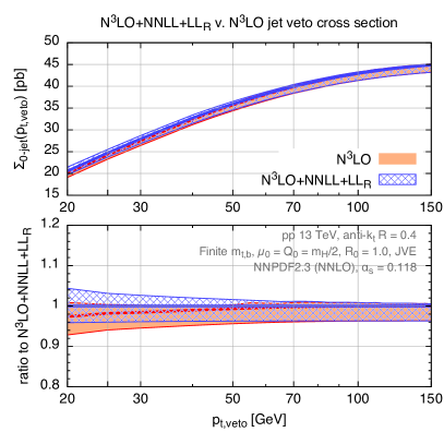
The predictions for jet-veto efficiency and the zero-jet cross section are summarised in Table 2, for two experimentally relevant choices. Results are reported both at fixed-order, and including the various resummation effects.
| LHC 13 TeV | ||||
|---|---|---|---|---|
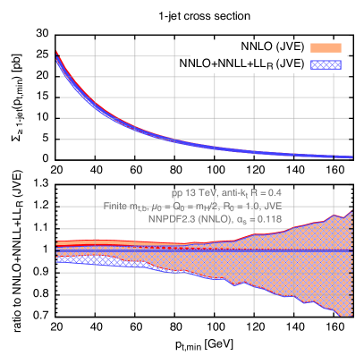
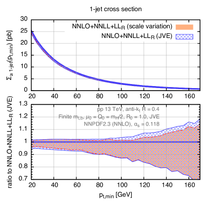
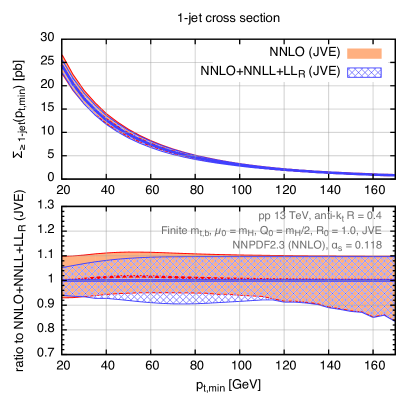
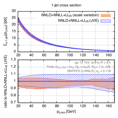
Figure 7 shows the inclusive one-jet cross section , for which the state-of-the-art fixed-order prediction is NNLO Boughezal:2015dra ; Boughezal:2015aha ; Caola:2015wna . The left-hand plot shows the comparison between the best prediction at NNLO+NNLL+LLR, and the fixed-order at NNLO. Both uncertainty bands are obtained with the JVE method outlined in Sec. 2.3. We observe that the effect of the resummation on the central value at moderately small values of is at the percent level. Moreover, the inclusion of the resummation leads to a slight increase of the theory uncertainty in the small transverse momentum region.
The right-hand plot of Fig. 7 shows our best prediction with uncertainty obtained with the JVE method, compared to the case of just scale (i.e. , , ) variations. We observe a comparable uncertainty both at small and at large transverse momentum, which indicates that the JVE method is not overly conservative in the tail of the distribution. We have observed that the same features persist for the corresponding differential distribution. Table 3 contains the predictions for the inclusive one-jet cross section for two characteristic choices.
| LHC 13 TeV | ||
|---|---|---|
4 Conclusions
In this article we have presented new state-of-the-art, N3LO+NNLL+LLR, predictions for the jet-veto efficiency and the zero-jet cross section in gluon-fusion induced Higgs production, as well as NNLO+NNLL+LLR results for the inclusive one-jet cross section. The results, shown for 13 TeV LHC collisions, incorporate recent advances in the fixed-order calculation of the total cross section Anastasiou:2015ema , the fixed-order calculation of the one-jet cross section Boughezal:2015dra ; Boughezal:2015aha ; Caola:2015wna and the resummation of small- effects Dasgupta:2014yra . They also include the earlier NNLL jet resummation Banfi:2012jm including finite quark mass effects Banfi:2013eda . Uncertainties have been determined using the jet-veto efficiency method, which has been updated here to take into account the good perturbative convergence observed with the new fixed-order calculations.
Results for the jet-veto efficiency and zero-jet cross section for central scale choices of and are reported in tables 2 and 5, respectively. With our central scale choice, , we find that the inclusion of the new calculations decreases the jet-veto efficiency by 2% with respect to the NNLO+NNLL prediction, and it has a substantially smaller uncertainty, reduced from more than 10% to less than 5%.
In the zero-jet cross section, the reduction in the jet-veto efficiency is compensated by a similar increase in the total cross section due to the N3LO correction, resulting in a sub-percent effect. In comparison to the N3LO result, the matched N3LO+NNLL+LLR jet-veto efficiency and zero-jet cross section are about 2% larger, and have comparable () theoretical errors. The picture is different for a central scale , as discussed in appendix B. In this case the jet-veto efficiency at N3LO+NNLL+LLR decreases by more than 5% with respect to the NNLO+NNLL result, while it is in perfect agreement with the pure N3LO prediction. Perturbative uncertainties are considerably (moderately) reduced with respect to the NNLO+NNLL (N3LO) prediction. For the inclusive one-jet cross section, we find a similar impact of the resummation in the small region, and agreement with the fixed-order scale variation at large transverse momentum values.
We stress that other corrections are of the same order as the theoretical uncertainties obtained here. These involve electro-weak effects, exact quark-mass treatment beyond the orders currently known, and non-perturbative effects. Furthermore, we stress that the results quoted here do not account for PDF and strong coupling uncertainties, which also are at the few-percent level.
Code for performing the resummation and matching with fixed order predictions is publicly available in version 3 of the JetVHeto program JetVHeto .
Acknowledgements
FC would like to thank Kirill Melnikov and Markus Schulze for collaboration and exchanges concerning the Higgs plus one jet computation. GPS and FAD would like to thank Mrinal Dasgupta, Matteo Cacciari and Gregory Soyez for collaboration in the early stages of the small- resummation part of this work. We wish to thank Babis Anastasiou, Claude Duhr and Bernhard Mistlberger for interesting discussions regarding the total cross section, and Kirill Melnikov for comments on the manuscript. GZ is supported by the HICCUP ERC Consolidator grant. PM is supported by the Swiss National Science Foundation (SNF) under grant PBZHP2-147297. The work of AB is supported by Science and Technology Facility Council (STFC) under grant number ST/L000504/1. FAD is supported by the ILP LABEX (ANR-10-LABX-63) financed by French state funds managed by the ANR within the Investissements d’Avenir programme under reference ANR-11-IDEX-0004-02. GPS is supported in part by ERC Advanced Grant Higgs@LHC. The work of FD is supported by the Swiss National Science Foundation (SNF) under contract 200021-143781 and by the European Commission through the ERC grant “IterQCD”. AB and PM wish to thank CERN for hospitality, and FC, PM, GS and GZ would like to express a special thanks to the Mainz Institute for Theoretical Physics (MITP) for its hospitality and support while part of this work was carried out.
Appendix A Revisited JVE uncertainty prescription
In this paper we argued that the JVE method of ref. Banfi:2012yh ; Banfi:2012jm used to estimate uncertainties should be modified. In this appendix we wish to motivate why we revisited the JVE prescription. We will argue that, while the original JVE method was appropriate when it was proposed (i.e. when only the NNLO correction to the 0-jet cross section in Higgs production was known), now that the N3LO correction is available it would give rise to excessively conservative uncertainties.
It is useful to first recall the original JVE method. In refs. Banfi:2012yh ; Banfi:2012jm , to determine uncertainties in the NNLO+NNLL prediction, and were varied by a factor of 2 in either direction, requiring . Maintaining central values, was also varied by a factor of 2 and changed the matching scheme, from the scheme to schemes and as defined in Banfi:2012jm . The final uncertainty band was the envelope of these variations (cf. Banfi:2012yh ). Our new prescription differs from the old one in two important points:
-
•
only schemes and are used to probe the sensitivity to the matching scheme;
-
•
the range for the resummation scale variation is , as suggested originally in ref. Dasgupta:2002dc .
In the rest of this appendix we comment on both of these aspects.
The reason for having different schemes is that the efficiency is a ratio of the jet-vetoed cross section to the total cross section. Even at fixed order there is some freedom as to which perturbative terms one chooses to keep in the denominator, or alternatively expand out. Different matching formulae can then be constructed that reproduce the corresponding fixed-order expansions for the JVE efficiency. At N3LO, in addition to schemes and defined in Eqs. (4), one can introduce three further schemes:
| (20a) | ||||
| (20b) | ||||
| (20c) | ||||
The schemes differ only by terms beyond N3LO.111111Corresponding formulae for the matching schemes can be found in the documentation of JetVHeto-v3 JetVHeto . At NNLO there are just three schemes, , and , which respectively have , and in the denominator:
| (21a) | ||||
| (21b) | ||||
| (21c) | ||||
where, to avoid confusion, here we have explicitly added a “NNLO” label. In what follows, we will drop this label.121212Note that there is a natural correspondence between N3LO and NNLO schemes and .
To understand why we now restrict the scheme variation to schemes and , we first show in Fig. 8 a comparison between the NNLO jet-veto efficiency at 8 TeV and 13 TeV, where we plot the three different possible matching schemes at this order (for the central scale choice). Concentrating first on the absolute values of the efficiency, one sees that in schemes and there is a reduction in going from 8 to 13 TeV. This is consistent with the expectation of an increase in the fraction of events containing a jet when one goes to higher centre-of-mass energy. In contrast, the efficiency increases in scheme . This seems unphysical. The combination of the different behaviours of schemes and has the consequence of a very substantial increase in apparent uncertainty. Moreover, at sufficiently high scheme returns an unphysical efficiency .
The issues with scheme are to some extent understood, since scheme at NNLO is very sensitive to the convergence of the first correction in the perturbative expansion. It is well-known that the first terms for the Higgs cross section converge very poorly. In particular, the ratio of NLO to LO cross section contributions, , goes from about to between and .131313The ratio is further enhanced when mass effects are included. The difference between schemes and , on the other hand, is only sensitive to the size of the last perturbative order, hence we believe it provides useful, but not overly conservative, information on the uncertainty.
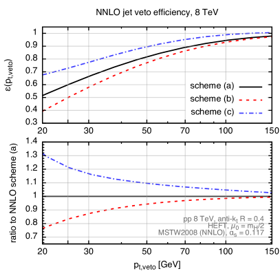
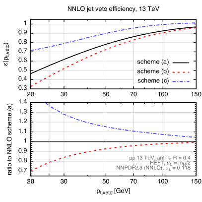
In order to study the impact of the new prescription for the efficiency scheme variation, in Fig. 9 we show the fixed-order efficiency at NNLO and N3LO, concentrating on the 13 TeV case, where the impact of scheme (at NNLO) and (at N3LO) is more pronounced. Fig. 9 shows the various efficiency schemes contributing at a given order according to the old JVE prescription. We see that at N3LO the spread between schemes and is comparable with the change in the efficiency from NNLO to N3LO, while the inclusion of additional schemes , and ) gives rise to a much larger uncertainty. This suggests that the old JVE prescription is overestimating uncertainties at this c.o.m. energy. This is even more true when including finite quark-mass effects (not shown here).
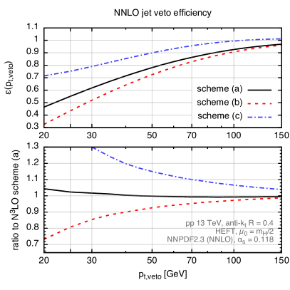
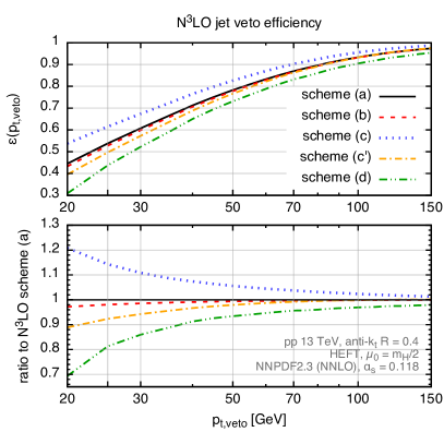
It is however also clear that, since the scheme prediction is obtained by computing the jet-veto efficiency at the central scale only, if the N3LO correction to the total cross section is accidentally very small at that scale, schemes and will return nearly identical values. Therefore, the corresponding scheme uncertainty will be very small. For our central scale the N3LO correction is in fact very small (2.4%) and, accordingly, the corresponding scheme spread in the right-hand plot of Fig. 9 is very small. To investigate whether this is a general feature of the new scheme prescription, one can examine the uncertainty band at a different central scale. We have done this in App. B, where it shown that in that case the scheme variation contributes significantly to the size of the theoretical uncertainty.
An alternative way to address the issue of accidentally small scheme variation is to introduce a prescription that probes the scheme variation at different scales (where the size of the N3LO corrections may be more sizeable). For instance, one could determine the scheme uncertainty by adding to the usual envelope the spread between schemes and at different scales. We therefore investigate the following prescription: to define the uncertainty band, we take the envelope of scheme with its set of 7 scale variations (and and variations) and additionally the 7 scale variations of
| (22) |
where we have included explicit subscript labels for the renormalisation and factorisation scales. By sampling Eq. (22) over 7 scale choices, one explores the maximum difference between schemes and (with identical scale choices for the two schemes) and applies that difference as an additional uncertainty relative to the result of scheme for its central scale choice . In this way one avoids the problem that the difference between schemes and may be accidentally small for the central scale choice. This approach also avoids the potential risk of double counting of uncertainties that would come were one simply to take the envelope of schemes and , each with 7 scale variations.
The comparison between the new JVE prescription to the procedure is shown in Fig 10. We see that the prescription gives rise to only marginally larger uncertainties. Moreover, we have found that the prescription gives rise to enlarged uncertainties in the tail of the leading jet distribution. For these reasons, and due the fact that this procedure is more cumbersome and relies on a non-standard method to assess the error, we do not adopt it as our default prescription.
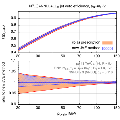
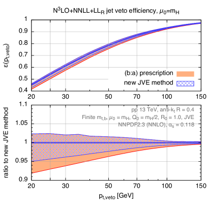
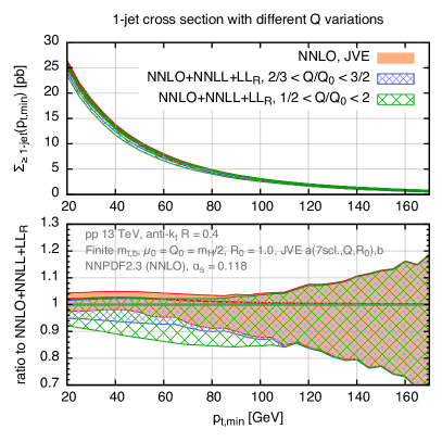
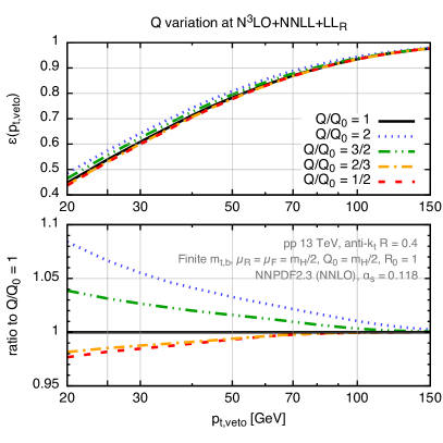
Besides the different efficiency scheme variation, another important difference between our new JVE prescription and the original one Banfi:2012yh is the range of variation for the resummation scale . Instead of varying it in the range as done originally, we now restrict ourselves to the smaller range . The main reason for this is that one wants the one-jet cross section at large to be insensitive to the resummation, therefore one should ensure that the resummation is correctly turned off at large values. The scale at which the resummation is turned off is determined by the resummation scale . Making the choice has the effect of starting the resummation in a region of relatively high , where the underlying soft and collinear approximations are far from being valid.
In the left-hand plot of Fig. 11 we show the one-jet cross section at NNLO+NNLL+LLR with uncertainties obtained with the new formulation of the JVE method both with a variation range of (green/hatched band) and (blue/hatched). The fixed order result (red/solid) is also shown for comparison. We observe that while the effect of resummation on the central value is very moderate, the band obtained with the old variation range is substantially larger all the way up to . The right-hand plot of Fig. 11 shows the jet-veto efficiency at N3LO+NNLL+LLR for the values of the resummation scale used in the old (, ) and in the new (, ) prescription for the JVE method. While the curve corresponding to the upper variation changes significantly when reducing from to , the curve corresponding to the lower edge is largely unaffected by the change in the variation range. The insensitivity to the choice of the lower end of the range for motivates a simple symmetric choice for the resummation scale range.
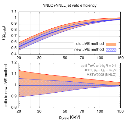
Finally, it is interesting to see how the original prediction of ref. Banfi:2012jm changes with the new prescription for the JVE uncertainty. Fig. 12 shows the comparison between the old and new JVE methods for the NNLO+NNLL efficiency at 8 TeV. We observe that the new prescription leads to a reduction of the upper part of the uncertainty band. At low values of this reduction is mainly driven by the reduction in the variation range (cf. Fig. 11), while at large scheme gives a significant contribution to the theoretical uncertainty (cf. Fig. 8). To conclude this section, we remark that when the original formulation of the JVE method was proposed, the NNLO corrections showed a somewhat problematic convergence, therefore a more conservative approach to the uncertainty estimate seemed appropriate. Now that the computation of the N3LO correction shows a much better convergence of the perturbative series, extensive study has led us to believe that the new formulation of the JVE method is more appropriate.
Appendix B Choice of the central scale
Results presented in the main text are obtained using as a central scale choice. This choice, rather than , is motivated by the better convergence of the perturbative expansion and by the fact that soft emissions and virtual corrections that contribute substantially to the cross-section tend to have scales that are typically lower than . It is similar also to the choice of or that is often used in processes with more complex final states. Nevertheless it is interesting to examine how much our central results and the uncertainties change when is adopted as a central scale.
Table 4 shows the input numerical values for the total and one-jet cross section, with and without mass effects, up to , with uncertainties obtained through scale variation and using NNLO PDFs and using a central scale . These numbers are to be compared to those at scale , Table 1.
| LHC 13 TeV [pb] | ||||||
|---|---|---|---|---|---|---|
| EFT | ||||||
| -only | ||||||
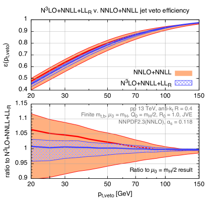
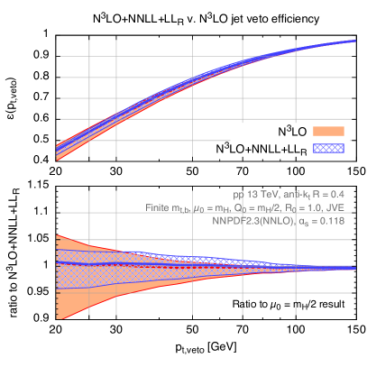
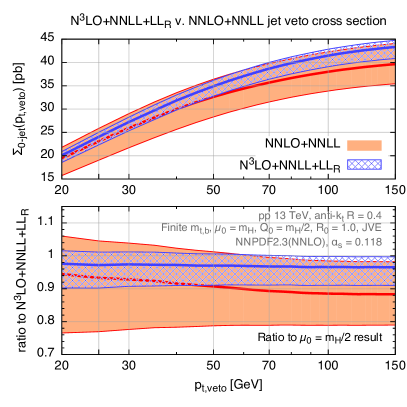
In Fig. 13 we show a comparison of the results to results (left) and to N3LO (right) at central scale . This figure is to be compared to the similar one at central scale , Fig. 5. It is clear that at scale uncertainties are somehow larger, this is particularly the case for the N3LO prediction. Accordingly, uncertainty bands overlap slightly better at scale . Still, the change in the central value at is very small when using rather than . The corresponding plots for the 0-jet cross section are shown in Fig. 14.
Results for the efficiency and 0-jet cross section are reported in Tab. 5.
| LHC 13 TeV | ||||
|---|---|---|---|---|
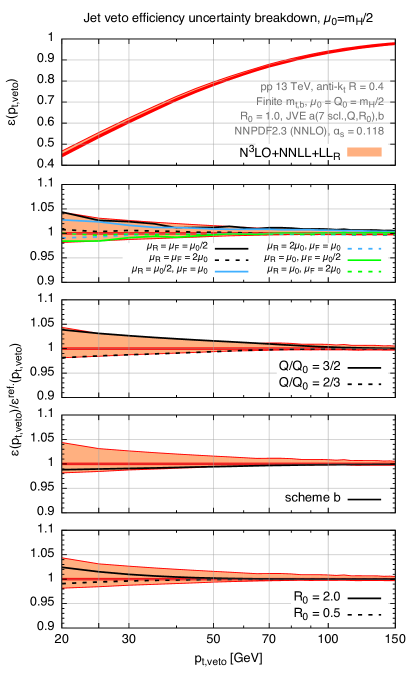
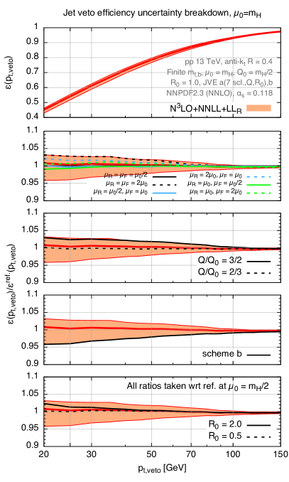
To gain insight into the differences between the two scale choices, Fig. 15 shows the breakdown into different sources of uncertainty using (left) and (right) as a central scale choice. We notice that for the central scale the full uncertainty band is determined by the scale variations (both and ), while scheme and variation give rise to a lower uncertainty. For central scale the upper edge of the band is still set by scale variation, while the lower one is determined by the scheme variation, and variation has still no impact on the final uncertainty band. The difference in the impact of the scheme variation at the two different scales is a consequence two facts: (a) at scale the N3LO correction is only a 2% correction, while it amounts to 9% at scale ; and (b) in our updated JVE approach, the scheme-variation is now sensitive only to the ambiguity of including (or not) the N3LO correction to the total cross section in the efficiency.
| LHC 13 TeV | ||
|---|---|---|
Next, in Fig. 16 we show the inclusive one-jet cross section (blue/hatched) compared to fixed-order at NNLO (left) and to the matched result with direct scale variation for the uncertainty as explained in the text (right) at central scale . Corresponding numerical values for the one-jet cross section are reported in Tab. 6. From the right-hand plot of Fig. 16, one notices that the JVE uncertainty band, especially its upper edge, is larger than scale variation even at transverse momenta of the order of . This larger uncertainty for the JVE result appears to be associated with the variation between schemes and , which differ by about over a range of , a consequence of the nearly difference between and that is visible in table 4. This effect is not present for the results with central scale , Fig. 7, where the difference between the two schemes is much smaller. However, for large values of the uncertainty on the results grows more rapidly, perhaps a consequence of the fact such a scale choice is not appropriate at high .
Appendix C Small- correction factor
In Ref. Dasgupta:2014yra , small- effects for jet vetoes were resummed through the introduction of a “fragmentation” function for the distribution of the momentum fraction carried by the hardest subjet resulting from the fragmentation of a gluon. The quantity used in Eq. (16) is the first logarithmic moment of this fragmentation function,
| (23) |
where the coefficients up to are the actual terms of the full Taylor expansion of , while those from to , given in table 7, are chosen so as to provide a good fit to the full numerical form for as calculated in Ref. Dasgupta:2014yra . Coefficients are tabulated both for and .141414The results of this paper use the values. As such, these higher order coefficients are not the actual values of the coefficients of the Taylor series for , since yet higher-order contributions might be partly absorbed in the fit. Eq. (C) reproduces the full all-order result at the per mil level in the range , which should be more than adequate for phenomenological applications.
| 133.55 | -478.55 | -1226.87 | 22549.99 | -77020.08 | |
| 100.69 | -352.10 | -858.44 | 15819.97 | -53597.50 |
For the purposes of matching, it is useful to have the expansion of up to . The and terms are known from previous work. Once one includes LLR resummation there is an additional term, which receives contributions from both the order and terms in Eq. (C), because itself has an all-order expansion in powers of . It is given by
| (24) |
References
- (1) G. Aad et al. [ATLAS Collaboration], Phys. Lett. B 716 (2013) 1 [arXiv:1207.7214 [hep-ex]].
- (2) S. Chatrchyan et al. [CMS Collaboration], Phys. Lett. B 716 (2013) 30 [arXiv:1207.7235 [hep-ex]].
- (3) G. Aad et al. [ATLAS Collaboration], Phys. Rev. D 92 (2015) 1, 012006 [arXiv:1412.2641 [hep-ex]].
- (4) S. Chatrchyan et al. [CMS Collaboration], JHEP 1401 (2014) 096 [arXiv:1312.1129 [hep-ex]].
- (5) A. Banfi, P. F. Monni, G. P. Salam and G. Zanderighi, Phys. Rev. Lett. 109 (2012) 202001 [arXiv:1206.4998 [hep-ph]].
- (6) I. W. Stewart, F. J. Tackmann, J. R. Walsh and S. Zuberi, Phys. Rev. D 89 (2014) 5, 054001 [arXiv:1307.1808].
- (7) T. Becher, M. Neubert and L. Rothen, JHEP 1310 (2013) 125 [arXiv:1307.0025 [hep-ph]].
- (8) C. Anastasiou, C. Duhr, F. Dulat, F. Herzog and B. Mistlberger, Phys. Rev. Lett. 114 (2015) 212001 [arXiv:1503.06056 [hep-ph]].
- (9) R. Boughezal, F. Caola, K. Melnikov, F. Petriello and M. Schulze, Phys. Rev. Lett. 115 (2015) 8, 082003 [arXiv:1504.07922 [hep-ph]].
- (10) R. Boughezal, C. Focke, W. Giele, X. Liu and F. Petriello, Phys. Lett. B 748 (2015) 5 [arXiv:1505.03893 [hep-ph]].
- (11) F. Caola, K. Melnikov and M. Schulze, Phys. Rev. D 92 (2015) 7, 074032 [arXiv:1508.02684 [hep-ph]].
- (12) M. Dasgupta, F. Dreyer, G. P. Salam and G. Soyez, JHEP 1504 (2015) 039 [arXiv:1411.5182 [hep-ph]].
- (13) A. Banfi, G. P. Salam and G. Zanderighi, JHEP 1206 (2012) 159 [arXiv:1203.5773 [hep-ph]].
- (14) M. Spira, A. Djouadi, D. Graudenz and P. M. Zerwas, Nucl. Phys. B 453 (1995) 17 [hep-ph/9504378].
- (15) M. Spira, Fortsch. Phys. 46 (1998) 203 [hep-ph/9705337].
- (16) R. Harlander and P. Kant, JHEP 0512 (2005) 015 [hep-ph/0509189].
- (17) C. Anastasiou, S. Beerli, S. Bucherer, A. Daleo and Z. Kunszt, JHEP 0701 (2007) 082 [hep-ph/0611236].
- (18) U. Aglietti, R. Bonciani, G. Degrassi and A. Vicini, JHEP 0701 (2007) 021 [hep-ph/0611266].
- (19) R. Bonciani, G. Degrassi and A. Vicini, JHEP 0711 (2007) 095 [arXiv:0709.4227 [hep-ph]].
- (20) T. Neumann and M. Wiesemann, JHEP 1411 (2014) 150 [arXiv:1408.6836 [hep-ph]].
- (21) H. Mantler and M. Wiesemann, Eur. Phys. J. C 73 (2013) 6, 2467 [arXiv:1210.8263 [hep-ph]].
- (22) M. Grazzini and H. Sargsyan, JHEP 1309 (2013) 129 [arXiv:1306.4581 [hep-ph]].
- (23) A. Banfi, P. F. Monni and G. Zanderighi, JHEP 1401 (2014) 097 [arXiv:1308.4634 [hep-ph]].
- (24) E. Bagnaschi, G. Degrassi, P. Slavich and A. Vicini, JHEP 1202 (2012) 088 [arXiv:1111.2854 [hep-ph]].
- (25) E. Bagnaschi and A. Vicini, arXiv:1505.00735 [hep-ph].
- (26) K. Hamilton, P. Nason and G. Zanderighi, JHEP 1505 (2015) 140 [arXiv:1501.04637 [hep-ph]].
- (27) I. W. Stewart and F. J. Tackmann, Phys. Rev. D 85 (2012) 034011 [arXiv:1107.2117 [hep-ph]].
- (28) M. Cacciari, G. P. Salam and G. Soyez, JHEP 0804, 063 (2008) [arXiv:0802.1189 [hep-ph]].
- (29) M. Cacciari, G. P. Salam and G. Soyez, Eur. Phys. J. C 72, 1896 (2012) [arXiv:1111.6097 [hep-ph]].
- (30) R. D. Ball, V. Bertone, S. Carrazza, C. S. Deans, L. Del Debbio, S. Forte, A. Guffanti and N. P. Hartland et al., Nucl. Phys. B 867 (2013) 244 [arXiv:1207.1303 [hep-ph]].
- (31) A. Buckley, J. Ferrando, S. Lloyd, K. Nordström, B. Page, M. Rüfenacht, M. Schönherr and G. Watt, Eur. Phys. J. C 75 (2015) 3, 132 [arXiv:1412.7420 [hep-ph]].
- (32) G. Bozzi, S. Catani, D. de Florian and M. Grazzini, Nucl. Phys. B 737 (2006) 73 [hep-ph/0508068].
- (33) T. Becher and M. Neubert, Eur. Phys. J. C 71 (2011) 1665 [arXiv:1007.4005 [hep-ph]].
- (34) M. Dasgupta and G. P. Salam, JHEP 0208 (2002) 032 [hep-ph/0208073].
- (35) R. W. L. Jones, M. Ford, G. P. Salam, H. Stenzel and D. Wicke, JHEP 0312 (2003) 007 [hep-ph/0312016].
- (36) F. J. Tackmann, J. R. Walsh and S. Zuberi, Phys. Rev. D 86 (2012) 053011 [arXiv:1206.4312 [hep-ph]].
- (37) S. Alioli and J. R. Walsh, JHEP 1403 (2014) 119 [arXiv:1311.5234 [hep-ph]].
- (38) G. Aad et al. [ATLAS and CMS Collaborations], arXiv:1503.07589 [hep-ex].
- (39) G. P. Salam and J. Rojo, Comput. Phys. Commun. 180 (2009) 120 [arXiv:0804.3755 [hep-ph]].
- (40) S. Actis, G. Passarino, C. Sturm and S. Uccirati, Phys. Lett. B 670 (2008) 12 [arXiv:0809.1301 [hep-ph]].
- (41) C. Anastasiou, R. Boughezal and F. Petriello, JHEP 0904 (2009) 003 [arXiv:0811.3458 [hep-ph]].
- (42) W. Y. Keung and F. J. Petriello, Phys. Rev. D 80 (2009) 013007 [arXiv:0905.2775 [hep-ph]].
- (43) https://jetvheto.hepforge.org/.