Symmetries and control in generative neural nets.

Abstract

We study generative nets which can control and modify observations, after being trained on real-life datasets. In order to zoom-in on an object, some spatial, color and other attributes are learned by classifiers in specialized attention nets. In field-theoretical terms, these learned symmetry statistics form the gauge group of the data set. Plugging them in the generative layers of auto-classifiers-encoders (ACE) appears to be the most direct way to simultaneously: i) generate new observations with arbitrary attributes, from a given class; ii) describe the low-dimensional manifold encoding the “essence” of the data, after superfluous attributes are factored out; and iii) organically control, i.e., move or modify objects within given observations. We demonstrate the sharp improvement of the generative qualities of shallow ACE, with added spatial and color symmetry statistics, on the distorted MNIST and CIFAR10 datasets.

1 Introduction

1.1 Generativity and control.

Generating plausible but unseen previously observations appears, at least chronologically, to have been one of the hardest challenges for artificial neural nets. A generative net can “dream-up” new observations $\{\hat{\mathbf{x}}_{\nu}\}$, each a vector in a high-dimensional space $\mathbb{R}^{N}$, by sampling from a white noise probability density $p(\mathbf{z})$. This model density resides on a preferably low-dimensional space of latent variables $\mathbf{z}$ = $\{\mathbf{z}^{(\kappa)}\}_{\kappa=1}^{N_{lat}}$. In order to create plausible new observations, the latent manifold has to encode the complexity of the set of $P$ training observations $\{\mathbf{x}_{\mu}\}_{\mu=1}^{P}$ $\subset\mathbb{R}^{N}$.

Generativity has a lot more to it than “dreaming-up” new random observations. It is at the heart of the control skills of a neural net. Visual biological nets, for example, capture existential motor information like location/shape and other attributes of an object and can act on it by moving or modifying it deterministically. Asking for this data compression to be as compact and low-dimensional as possible is therefore not only a general minimalist requirement. Learning and mastering control is a gradual process, which naturally starts by seeking and exploring only a few degrees of freedom.

Moreover, the ability to modify an object implies an ability to first and foremost reconstruct it, with various degrees of precision. Not unlike human creativity, a fully generative net has to balance out and minimize terms with non-compatible objectives: a) a generative error term, which is responsible for converting random noise into plausible data, on the one hand, and b) a reconstruction error term which is responsible for meticulous reconstruction of existing objects, on the other.

1.2 Learning from real-life data.

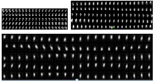
From the recent crop of generative nets, section 2, only one appears to offer this desirable reconstruction via a low-dimensional latent manifold: the variational auto-encoders (VAE) Kingma & Welling (2014), Rezende et al. (2014). Their subset called Gibbs machines, has also far-reaching roots into information geometry and thermodynamics, which come in very handy. They perform well on idealized visual data sets like MNIST LeCun et al. (1998). Unfortunately, like the other generative nets, they do not cope well with more realistic images, when objects are spatially varied or, if there is heavy clutter in the background. These traits are simulated in the rotated-translated-scaled (RTS) MNIST and translated-cluttered (TC) MNIST, Appendix B. We highlight the shortcomings of basic generative nets on Figure 1, for the simplest case of one-dimensional latent manifold per class. While simulating wonderfully on the original MNIST (top-left), even with $N_{lat}=1$, the net fails miserably to learn the distorted data: The randomly “dreamed-up” samples $\{\hat{\mathbf{x}}_{\nu}\}$ are blurred and not plausible (top-right and bottom). Low latent dimensionality is not the culprit: latent manifolds with dimensions $N_{lat}\geq 100$ do not yield much better results.

Figure 1: One-dimensional latent manifold for some of the MNIST classes, each row corresponding to a separate class. Top Left. Original MNIST, on 28x28 canvas. Top Right. RTS MNIST, on 42x42 canvas. Bottom. TC MNIST, on 60x60 canvas, Appendix B. The net is a generative ACE in creative regime Georgiev (2015). The latent layer is one-dimensional per class, traversed by an equally spaced deterministic grid $\{\sigma_{s}\}_{s=1}^{20}$, $-4\leq\sigma_{s}\leq 4$. Implementation details in Appendix A.

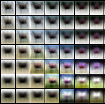
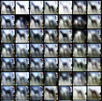
For the real-life CIFAR10 dataset, Krizhevsky (2009), the latent two-dimensional manifold of the class of horses, produced by the same architecture, is on the left of Figure 3. The training dataset has horses of different colors, facing both left and right, so the latent manifold tends to produce two-headed vague shapes of different colors.

1.3 “A horse, a horse! My kingdom for a horse!”

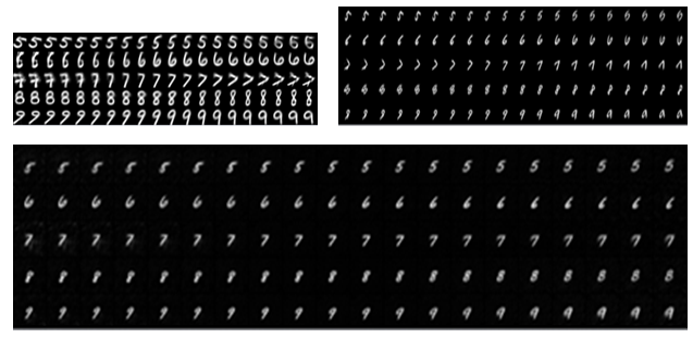
In order to get the horses back, we invoke the Gibbs thermodynamic framework. It allows adding non-energy attributes to the sampling distribution and modifying them, randomly or deterministically. These symmetry statistics, like location, size, angle, color etc, are factored-out at the start and factored back-in at the end. The auto-classifier-encoder (ACE) net with symmetry statistics was suggested in Georgiev (2015) and detailed in section 4 here. The latent manifolds it produces, for the above three MNIST datasets, are on Figure 2:

Figure 2: The analog of Figure 1, but produced by ACE with spatial symmetry statistics. For the original MNIST (top left), the size variation disappeared from the digit 5 class and the digit 7 class acquired a dash. In other words, one sees more genuine “core style” variation, even with one latent dimension only. Implementation details in Appendix A.

With distortions and clutter factored out, the quotient one-dimensional latent manifold is clear and legible. The factorization is via transformations from the affine group $\mathbf{Aff}(2,\mathbb{R})$, which plays the role of the gauge group in field theory. The spatial symmetry statistics are the transformations parameters, computed via another optimizer net. The CIFAR10 horse class manifold, generated by ACE with spatial symmetry statistics, is on the right of Figure 3. We have horse-like creatures, which morph into giraffes as one moves up the grid!

Figure 3: Left. Latent manifold for the horse class in CIFAR10, using a shallow ACE, with two latent dimensions per class, without symmetry statistics. These simulated images are from a 7x7 central segment of an equally spaced deterministic 30x30 grid $\{\sigma_{s},\tau_{s}\}_{s=1}^{30}$, $-6\leq\sigma_{s},\tau_{s}\leq 6$. Right. Same, but generated by shallow ACE with spatial symmetry statistics (implementation details in Appendix A). To appreciate them, compare to other generative nets: Figure 2 (c) in Goodfellow et al. (2014), or Figure 3 (d) in Sohl-Dickstein et al. (2015). The improvement in Denton et al. (2015) is due to so-called Laplacian pyramids, and can be overlayed on any core generative model.

The first successful application of Lie algebra symmetries to neural nets was in Simard et al. (2000). The recent crop of spatial attention nets Jadeberg et al. (2015), Gregor et al. (2015), Sermanet et al. (2014), Ba et al. (2014) optimize spatial symmetry statistics, corresponding to a given object inside an observation. An efficient calculation of symmetry statistics, for multiple objects, requires a classifier. Hence, generation and reconstruction on real-life datasets lead to an auto-encoder/classifier combo like ACE. Supplementing auto-encoders with affine transforms was first proposed in Hinton et al. (2011), where spatial symmetry statistics were referred to as “capsules”. As suggested there, hundreds and thousands of capsules can in principle be attached to feature maps. Current attention nets produce one set of symmetry statistics per object (inside an observation). Incorporating convolutional feature maps in the encoder, and sampling from symmetry statistics at various depths, is yet to be engineered well for deep generative nets, see open problems 1, 2, section 5. Results from a shallow convolutional ACE are on Figure 4.

Figure 4: Same as Figure 3, but with the two fully-connected encoder hidden layers replaced by convolutional ones. Corresponding deconvolution layers, Zeiler & Fergus (2014), are added to decoder. Left. Shallow ACE with spatial symmetry statistics only. Right. Shallow ACE with both spatial and color symmetry statistics: as a result, the green background is subdued. Implementation details in Appendix A.

Spatial symmetry statistics are vital in biological nets and can in principle be traced down experimentally. Feedback loops for attention data, vaguely reminiscent of Figure 5, have been identified between higher- and lower-level visual areas of the brain, Sherman (2005), Buffalo et al. (2010).

For colored images, one also needs the color symmetry statistics, forming a semigroup of non-negative 3x3 matrices in the stochastic group $\mathbf{S}(3,\mathbb{R})$. As shown on the right of Figure 4, they help subdue the background color, and perhaps, more. In particle physics parlance, three-dimensional color images are described by chromodynamics with a minimum gauge group $\mathbf{Aff}(3,\mathbb{R})$ $\times~{}\mathbf{S}(3,\mathbb{R})$.

The rest of the paper is organized as follows: section 2 briefly overviews recent generative nets and details VAE-s objective function; section 3 outlines the theoretical framework of generative nets with control, highlighting the connections with information geometry and thermodynamics; section 4 presents the enhanced ACE architecture; the Appendices offer implementation and dataset details.

2 Generative nets and the latent manifold.

Latent manifold learning was pioneered for modern nets in Rifai et al. (2012). When a latent sample $\mathbf{z}_{\nu}$ is chosen from a model density $p(\mathbf{z})$, a generative net decodes it into a simulated observation $\hat{\mathbf{x}}_{\nu}$, from a corresponding model density $q(\hat{\mathbf{x}})$. There are two scenarios:

a) the net has reconstruction capabilities, hence $q(\mathbf{x})$ can in theory be evaluated on the training and testing observations $\{\mathbf{x}_{\mu}\}$. The objective is to minimize the so-called cross-entropy or negative log-likelihood, i.e., the expectation $\mathbf{E}(-\log q(\mathbf{x}))_{r(\mathbf{x})}$, where $\mathbf{E}()_{r()}$ is an expectation with respect to the empirical density $r()$. Recently proposed reconstructive generative nets are: i) the generalized denoising auto-encoders (DAE) Bengio et al. (2013), ii) the generative stochastic networks (GSN) Bengio et al. (2014), iii) the variational auto-encoders introduced above, iv) the non-linear independent component estimation (NICE) Dinh et al. (2014), and v) Sohl-Dickstein et al. (2015). Except for NICE, the log-likelihood can not be exactly evaluated in practice, and is hence approximated. The first two models proxy $q(\mathbf{x})$ with a certain conditional density $q(\mathbf{x}|\tilde{\mathbf{x}})$ and a Markov chain for the corrupted data $\tilde{\mathbf{x}}$. The variational auto-encoders proxy the negative log-likelihood by a variational upper bound $\mathcal{U}(-\log q(\mathbf{x}))$. Method v) conjures up a forward diffusion process from $q(\mathbf{x})$ to $p(\mathbf{z})$ and uses the backward diffusion process to “dream-up” new observations $\{\hat{\mathbf{x}}_{\nu}\}$.

b) the net has no reconstruction capabilities, hence one has to resort to an interpolation $q(\hat{\mathbf{x}})$ $\rightarrow$ $\hat{q}(\mathbf{x})$, in order to evaluate $q()$ on the training and testing observations $\{\mathbf{x}_{\mu}\}$. The objective is to minimize directly or indirectly the negative log-likelihood $\mathbf{E}(-\log\hat{q}(\mathbf{x}))_{r(\mathbf{x})}$. Recent such model is the generative adversarial network (GAN) Goodfellow et al. (2014). It minimizes indirectly the above negative log-likelihood by combining a generative and a discriminative net, the latter tasked with distinguishing between the “dreamed-up” observations $\{\hat{\mathbf{x}}_{\nu}\}$ and training observations $\{\mathbf{x}_{\mu}\}$.

Of these models, only the variational auto-encoders and the generative adversarial networks are designed to handle a low-dimensional latent manifold. As argued in sub-section 1.1, reconstruction, i.e. scenario a), is an indispensable part of the control skill set, hence we are left with the variational auto-encoder approach. As all generative nets, variational auto-encoders work in two regimes:

• creative regime, with no data clamped onto the net and sampling from $p(\mathbf{z})$, and

• non-creative regime, with the training or testing observations $\{\mathbf{x}_{\mu}\}$ fed to the input layer of the net. Variational auto-encoders sample in this regime from a different closed-form conditional posterior model density $p(\mathbf{z}|\mathbf{x}_{\mu})$.

In order to do reconstruction, variational auto-encoders also introduce a conditional model reconstruction density $p^{rec}(\mathbf{x}_{\mu}|\mathbf{z})$. In non-creative regime, the reconstruction error at the output layer of the net is the expectation $\mathbf{E}(-\log p^{rec}(\mathbf{x}_{\mu}|\mathbf{z}))_{p(\mathbf{z}|\mathbf{x}_{\mu})}$. In the creative regime, we have a joint model density $p(\mathbf{x}_{\mu},\mathbf{z})$ $:=p^{rec}(\mathbf{x}_{\mu}|\mathbf{z})p(\mathbf{z})$. The data model density $q(\mathbf{x}_{\mu})$ is the implied marginal:

$$q(\mathbf{x}_{\mu})=\int p(\mathbf{x}_{\mu},\mathbf{z})d\mathbf{z}=\frac{p(\mathbf{x}_{\mu},\mathbf{z})}{q(\mathbf{z}|\mathbf{x}_{\mu})},$$ (2.1)

for some implied posterior conditional density $q(\mathbf{z}|\mathbf{x}_{\mu})$ which is generally intractable, $q(\mathbf{z}|\mathbf{x}_{\mu})$ $\neq p(\mathbf{z}|\mathbf{x}_{\mu})$. The full decomposition of our minimization target - the negative log-likelihood $-\log q(\mathbf{x}_{\mu})$ - is easily derived via the Bayes rules, Georgiev (2015), section 3:

$$-\log q(\mathbf{x}_{\mu})=\underbrace{\mathbf{E}(-\log p^{rec}(\mathbf{x}_{\mu}|\mathbf{z}))_{p(\mathbf{z}|\mathbf{x}_{\mu})}}_{reconstruction~{}error}+\underbrace{\mathcal{D}(p(\mathbf{z|x}_{\mu})||p(\mathbf{z}))}_{generative~{}error}-\underbrace{\mathcal{D}(p(\mathbf{z|x}_{\mu})||q(\mathbf{z|x}_{\mu}))}_{variational~{}error},$$ (2.2)

where $\mathcal{D}(||)$ is the Kullback-Leibler divergence. The reconstruction error measures the negative likelihood of getting $\mathbf{x}_{\mu}$ back, after the transformations and randomness inside the net. The generative error is the divergence between the generative densities in the non-creative and creative regimes. The variational error is an approximation error: it is the price variational auto-encoders pay for having a tractable generative density $p(\mathbf{z}|\mathbf{x}_{\mu})$ in the non-creative regime. It is hard to compute, although some strides have been made, Rezende & Mohamed (2015). For the Gibbs machines discussed below, it was conjectured that this error can be made arbitrary small, Georgiev (2015).

3 The theory. Connections with information geometry and thermodynamics.

A theoretical framework for universal nets was recently outlined in Georgiev (2015). Some of the constructs there, like the ACE architecture, appeared optional and driven solely by requirements for universality. We summarize and generalize the framework in the current context and argue that the ACE architecture, or its variations, are indispensable for generative reconstructive nets.

1. Information geometry and Gibbs machines: the minimization of the generative error in (2.2) leads to sampling from Gibbs a.k.a. exponential class of densities. It follows from the probabilistic or variational Pythagorean theorem, Chentsov (1968), which underlies modern estimation theory, and is pervasive in information geometry, Amari & Nagaoka (2000). In the case of Laplacian generative densities, and conditionally independent latent variables $\mathbf{z}$ $=\{z^{(\kappa)}\}_{\kappa=1}^{N_{lat}}$, one has:

   $$p(\mathbf{z|x}_{\mu})\sim e^{-\sum_{\kappa=1}^{N_{lat}}p^{(\kappa)}_{\mu}|z^{(\kappa)}-m^{(\kappa)}_{\mu}|},$$ (3.1)

   where the means $\{m_{\mu}^{(\kappa)}\}$ are symmetry statistics, the absolute value terms are sufficient statistics and the inverse scale momenta $\{p_{\mu}^{(\kappa)}\}$ are Lagrange multipliers, computed so as to satisfy given expectations of the sufficient statistics. The Gibbs density class leads to:

2. Thermodynamics and more symmetry statistics: The Gibbs class is also central in thermodynamics because it is maximum-entropy class and allows to add fluctuating attributes, other than energy. These additions are not cosmetic and fundamentally alter the dynamics of the canonical distribution, Landau & Lifshitz (1980), section 35. They can be any attributes: i) spatial attributes, as in the example below; ii) color attributes, as introduced in subsection 1.3, and others. For multiple objects, one needs specialized nets and a classifier to optimize them. This leads to:

3. Auto-classifiers-encoder (ACE) architecture, section 4: Since classification labels are already needed above, the latent manifold is better learned: i) via supervised reconstruction, and ii) with symmetry statistics used by decoder. This leads to:

4. Control: With symmetry statistics in the generative layer, the net can organically move or modify the respective attributes of the objects, either deterministically or randomly. The ACE architecture ensures that the modifications stay within a given class.

Example: An important special case in visual recognition are the spatial symmetry statistics, which describe the location, size, stance etc of an object. For a simple gray two-dimensional image $\mathbf{x}_{\mu}$ on $N$ pixels e.g., two of its spatial symmetry statistics are the coordinates $(h_{\mu},v_{\mu})$ of its center of mass, where the ”mass” of a pixel is its intensity. Assuming independence, one can embed a translational invariance in the net, multiplying (3.1) by the spatial symmetry statistics (SSS) conditional density:

$$p_{SSS}(\mathbf{z|x}_{\mu})\sim e^{-p^{(h)}_{\mu}|z^{(h)}-h_{\mu}|-p^{(v)}_{\mu}|z^{(v)}-v_{\mu}|},$$ (3.2)

where $z^{(h)},z^{(v)}$ are two new zero-mean latent random variables, responsible respectively for horizontal and vertical translation. If $(\mathbf{h},\mathbf{v})$ are the vectors of horizontal and vertical pixel coordinates, the image is centered at the input layer via the transform $(\mathbf{h},\mathbf{v})$ $\rightarrow$ $(\mathbf{h}-h_{\mu},\mathbf{v}-v_{\mu})$. This transformation is inverted, before reconstruction error is computed.

When rescaled and normalized, (3.2) is the quantum mechanical probability density of a free particle, in imaginary space/time and Planck constant $\hslash=1$. Furthermore, for every observation $\mathbf{x}_{\mu}$, there could be multiple or infinitely many latents $\{\mathbf{z}_{\mu}^{(\kappa)}\}_{\kappa=1}^{L}$, $L\leq\infty$, and $\mathbf{x}_{\mu}$ is merely a draw from a probability density $p^{rec}(\mathbf{x}_{\mu}|\mathbf{z})$. In a quantum statistics interpretation, latents are microscopic quantum variables, while observables like pixels, are macroscopic aggregates. Observations represent partial equilibria of independent small parts of the expanded (by a factor of $L$) data set.

4 ACE with symmetry statistics.

Figure 5: ACE architecture with symmetry statistics: compared to the basic generative ACE from Georgiev (2015), new components are in blue oval. $\mathbf{AE}$ stands for “auto-encoder”, $\mathbf{SSN}$ stands for “symmetry statistics net”, $\mathbf{C}$ stands for “classifier”. The arrow from the symmetry statistics to the $\mathbf{AE}$ latent variables indicates that one can sample from the former as well. The arrow from the symmetry statistics to the $\mathbf{AE}$ output layer indicates that one has to invert the transformation from box 0.4, before computing reconstruction error. On the test set, the class probabilities are provided by the classifier as in (4.1), hence the dashed lines.

The ACE architecture with symmetry statistics is on Figure 5. As in the basic ACE, training is supervised i.e. labels are used in the auto-encoder and every class has a dedicated decoder, with unimodal sampling in the generative layer of each class. The sampling during testing is instead from a mixture of densities, with mixture weights $\{\omega_{\mu,c}\}_{c=1}^{N_{C}}$ for the $\mu$-th observation, for class $c$, produced by the classifier. The posterior densitiy from section 2 becomes:

$$p(\mathbf{z}|\mathbf{x}_{\mu})=\sum_{c=1}^{N_{C}}\omega_{\mu,c}p(\mathbf{z}|\mathbf{x}_{\mu},c).$$ (4.1)

After interim symmetry statistics are computed in box 0.3 on Figure 5, they are used to transform the input (box 0.4), before it is sent for reconstruction and classification. The inverse transformation is applied right before the calculation of reconstruction error.

Plugging the symmetry statistics in the latent layers allows to deterministically control the reconstructed observations. Alternatively, sampling randomly from the symmetry statistics, organically “augments” the training set. External augmentation is known to improve significantly a net’s classification performance Ciresan et al. (2012), Krizhevsky et al. (2012). This in turn improves the quality of the symmetry statistics and creates a virtuous feedback cycle.

5 Open problems.

1. Test experimentally deep convolutional ACE-s, with (shared) feature maps, both in the classifier and the encoder. From feature maps at various depths, produce corresponding generative latent variables. Add symmetry statistics to latent variables at various depths.

2. Produce separate symmetry statistics for separate feature maps in generative nets, in the spirit of Hinton et al. (2011).

Acknowledgments

We appreciate discussions with Nikola Toshev, Stefan Petrov and their help with CIFAR10.

Appendix A Implementation.

All cited nets are implemented on the Theano platform, Bastien et al. (2012). Optimizer is Adam, Kingma & Ba (2015), stochastic gradient descent back-propagation, learning rate = 0.0015 for MNIST and 0.0005 for CIFAR10, decay = 50 epochs, batch size = 250. We used only one standard set of hyper-parameters per dataset and have not done hyper-parameter optimizations. Convolutional weights are initialized uniformly in $(-1,1)$ and normalized by square root of the product of dimensions. Non-convolutional weight initialization is as in Georgiev (2015).

Figure 1: Auto-encoder branch as in Georgiev (2015) Figure 9, Gaussian sampling. Classifier branch is convolutional, with 3 hidden layers, with 32-64-128 3x3 filters respectively, with 2x2 max-poolings and a final fully-connected layer of size 700; dropout is 0.2 in input and 0.5 in hidden layers. Figure 2: Same auto-encoder and classifier as in Figure 1. A symmetry statistics localization net, as in Jadeberg et al. (2015), produces six affine spatial symmetry statistics (box 0.2 in Figure 5). This net has 2 convolutional hidden layers, with 20 5x5 filters each, with 2x2 max-poolings between layers, and a fully-connected layer of size 50. Figure 3: Layer sizes 3072-2048-2048-(2x10)-(2048x10)-(2048x10)-(3072x10) for the auto-encoder branch, same classifier as in Fig 2. The symmetry statistics net has 2 convolutional hidden layers, with 32-64 3x3 filters respectively, with 2x2 max-poolings between layers, and a fully-connected layer of size 128. Figure 4: Two convolutional layers replace the first two hidden layers in the encoder, with 32-64 5x5 filters respectively. The two corresponding deconvolution layers are at the end of the decoder. Layer size 2048 is reduced to 1500 in the auto-encoder, Laplacian sampling, rest is the same as in Figure 3.

Appendix B Distorted MNIST.

The two distorted MNIST datasets replicate Jadeberg et al. (2015), Appendix A.3, although different random seeds and implementation details may cause differences. The rotated-translated-scaled (RTS) MNIST is on 42x42 canvas with random +/- 45^∘ rotations, +/- 7 pixels translations and $1.2$/$0.7$ scaling. The translated-cluttered (TC) MNIST has the original image randomly translated across a 60x60 canvas, with 6 clutter pieces of size 6x6, extracted randomly from randomly picked other images and added randomly to the background.

References

- Amari & Nagaoka (2000) Amari, S. and Nagaoka, H. Methods of Information Geometry. 2000.
- Ba et al. (2014) Ba, Jimmy, Mnih, Volodymyr, and Kavukcuoglu, Koray. Multiple object recognition with visual attention. In ICLR, 2014.
- Bastien et al. (2012) Bastien, Frédéric, Lamblin, Pascal, Pascanu, Razvan, Bergstra, James, Goodfellow, Ian J., Bergeron, Arnaud, Bouchard, Nicolas, and Bengio, Yoshua. Theano: new features and speed improvements, 2012.
- Bengio et al. (2013) Bengio, Yoshua, Yao, Li, Alain, Guillaume, and Vincent, Pascal. Generalized denoising auto-encoders as generative models. In NIPS, volume 26, 2013.
- Bengio et al. (2014) Bengio, Yoshua, Thibodeau-Laufer, Eric, and Yosinski, Jason. Deep generative stochastic networks trainable by backprop. In ICML, 2014.
- Buffalo et al. (2010) Buffalo, E.A., Fries, P., Landman, R., Liang, H., and Desimone, R. A backward progression of attentional effects in the ventral stream. Proc. Nat. Acad. Sci., 107(1), 2010.
- Chentsov (1968) Chentsov, N.N. Nonsymmetrical distance between probability distributions, entropy and the theorem of Pythagoras. Mathematical notes of the Academy of Sciences of the USSR, 4(3), 1968.
- Ciresan et al. (2012) Ciresan, Dan, Meier, Ueli, and Schmidhuber, Juergen. Multi-column deep neural networks for image classification, 2012. arXiv:1202.2745.
- Denton et al. (2015) Denton, Emily, Chintala, Soumith, Szlam, Arthur, and Fergus, Rob. Deep generative image models using a laplacian pyramid of adversarial networks, 2015. arXiv:1506.05751.
- Dinh et al. (2014) Dinh, Laurent, Krueger, David, and Bengio, Yoshua. NICE: Non-linear independent components estimation, 2014. arXiv:1410.8516.
- Georgiev (2015) Georgiev, Galin. Towards universal neural nets: Gibbs machines and ACE, 2015. arXiv:1508.06585v3.
- Goodfellow et al. (2014) Goodfellow, Ian J., Pouget-Abadie, Jean, Mirza, Mehdi, Xu, Bing, Warde-Farley, David, Ozair, Sherjil, Courville, Aaron, and Bengio, Yoshua. Generative adversarial networks, 2014. arXiv:1406.2661.
- Gregor et al. (2015) Gregor, Karol, Danihelka, Ivo, Graves, Alex, and Wierstra, Daan. DRAW: A recurrent neural network for image generation, 2015. arXiv:1502.04623.
- Hinton et al. (2011) Hinton, Geoffrey, Krizhevsky, Alex, and Wang, S. Transforming auto-encoders. In ICANN, 2011.
- Jadeberg et al. (2015) Jadeberg, Max, Symonyan, Karen, Zisserman, Andrew, and Kavukcuoglu, Koray. Spatial transformer networks, 2015. arXiv:1412.6980.
- Kingma & Ba (2015) Kingma, Diederik and Ba, Jimmy. Adam: A method for stochastic optimization. In ICLR, 2015.
- Kingma & Welling (2014) Kingma, Durk P. and Welling, Max. Auto-encoding variational Bayes. In ICLR, 2014.
- Kingma et al. (2014) Kingma, Durk P., Rezende, Danilo J., Mohamed, Shakir, and Welling, Max. Semi-supervised learning with deep generative models. 2014. arXiv:1406.5298.
- Krizhevsky (2009) Krizhevsky, Alex. Learning multiple layers of features from tiny images. Technical report, 2009.
- Krizhevsky et al. (2012) Krizhevsky, Alex, Sutskever, Ilya, and Hinton, Geoffrey. Imagenet classification with deep convolutional neural networks. In NIPS, volume 25, 2012.
- Landau & Lifshitz (1980) Landau, L.D. and Lifshitz, E.M. Statistical Physics, Part 1, 3rd edition. 1980.
- LeCun et al. (1998) LeCun, Yann, Cortes, Corinna, and Burges, Christopher J.C. MNIST handwritten digit database, 1998. URL http://yann.lecun.com/exdb/mnist/.
- Poole (1995) Poole, David. The stochastic group. American Mathematical Monthly, 102, 1995.
- Rezende & Mohamed (2015) Rezende, Danilo J. and Mohamed, Shakir. Variational inference with normalizing flows, 2015. arXiv:1505.05770.
- Rezende et al. (2014) Rezende, Danilo J., Mohamed, Shakir, and Wierstra, Daan. Stochastic backpropagation and approximate inference in deep generative models. In JMLR, volume 32, 2014.
- Rifai et al. (2012) Rifai, Salah, Bengio, Yoshua, Dauphin, Yann, and Vincent, Pascal. A generative process for sampling contractive auto-encoders. In ICML, 2012.
- Sermanet et al. (2014) Sermanet, Pierre, Eigen, David, Zhang, Xiang, Mathieu, Michaël, Fergus, Rob, and LeCun, Yann. Overfeat: Integrated recognition, localization and detection using convolutional networks. 2014.
- Shakespeare (1592) Shakespeare, William. King Richard the Third, Act V, Scene IV. 1592.
- Sherman (2005) Sherman, Murray. Thalamic relays and cortical functioning. Progress in Brain Research, 149, 2005.
- Simard et al. (2000) Simard, P., Cun, Y. Le, Denker, J., and Victorri, B. Transformation invariance in pattern recognition: Tangent distance and propagation. Int. J. Imag. Syst. Tech., 11(3), 2000.
- Sohl-Dickstein et al. (2015) Sohl-Dickstein, Jascha, Weiss, Eric, Maheswaranathan, Niru, and Ganguli, Surya. Deep unsupervised learning using nonequilibrium thermodynamics. In ICML, volume 37, 2015.
- Zeiler & Fergus (2014) Zeiler, Matthew D. and Fergus, Rob. Visualizing and understanding convolutional networks. In ECCV, 2014.