Comparison of canonical and microcanonical definitions of entropy
Abstract
For more than 100 years, one of the central concepts in statistical mechanics has been the microcanonical ensemble, which provides a way of calculating the thermodynamic entropy for a specified energy. A controversy has recently emerged between two distinct definitions of the entropy based on the microcanonical ensemble: (1) The Boltzmann entropy, defined by the density of states at a specified energy, and (2) The Gibbs entropy, defined by the sum or integral of the density of states below a specified energy. A critical difference between the consequences of these definitions pertains to the concept of negative temperatures, which by the Gibbs definition cannot exist. In this paper, we call into question the fundamental assumption that the microcanonical ensemble should be used to define the entropy. We base our analysis on a recently proposed canonical definition of the entropy as a function of energy. We investigate the predictions of the Boltzmann, Gibbs, and canonical definitions for a variety of classical and quantum models. Our results support the validity of the concept of negative temperature, but not for all models with a decreasing density of states. We find that only the canonical entropy consistently predicts the correct thermodynamic properties, while microcanonical definitions of entropy, including those of Boltzmann and Gibbs, are correct only for a limited set of models. For models which exhibit a first-order phase transition, we show that the use of the thermodynamic limit, as usually interpreted, can conceal the essential physics.
pacs:
05.70.-a, 05.20.-yI Introduction
The thermodynamic entropy is unique, and provides a complete description of the macroscopic properties of a system[1]. Nevertheless, its definition is still the subject of some dispute. Recently, a controversy has emerged between two distinct microcanonical definitions: (1) The Boltzmann entropy, given by the density of states at a specified energy[2, 3, 4, 5, 6], and (2) The Gibbs entropy, given by the sum or integral of the density of states below a specified energy[7, 8]. A critical difference between the consequences of these definitions pertains to the concept of negative temperatures[9, 10, 11], which by the Gibbs definition, cannot exist. The advocates of the Gibbs entropy reject negative temperatures, claiming that they are inconsistent with thermodynamic principles [12, 13, 14, 15, 16, 17, 18], while other authors have argued that thermodynamics is consistent with negative temperatures, and a different definition of entropy can give correct thermodynamic predictions when the Gibbs entropy does not[19, 20, 21, 22, 23, 24, 25, 26, 27, 28, 29, 30, 31, 32, 33, 34].
A related issue that has been raised is whether the limit of an infinite system (thermodynamic limit) is essential to thermodynamics[15, 16, 17, 35, 36, 37, 38]. We take the position that, while the approximation of an infinite system can be useful for certain calculations, it is also necessary for any theoretical approach to specify how to calculate the thermal properties of finite systems.
For example, a gas in a container that can adsorb particles on its walls has both interesting (non-extensive) physics and practical applications. However, in the limit of an infinite system the contribution of the walls diverges more slowly than the contributions of the bulk. As the thermodynamic limit is usually represented, the system appears to be extensive, and the effect of the walls is lost. We will show that in a similar way, the thermodynamic limit can obscure the essential physics of first-order transitions, and we suggest an alternate representation of the thermodynamic limit.
It has been claimed that thermodynamics should also apply to systems as small as a single particle[12, 13, 14, 15, 16, 17]. While we agree that thermodynamics should apply to finite systems, the predicted measurements of such systems should be unique. This requires a large number of particles so that the measured macroscopic variables have relative fluctuations smaller than the accuracy of the measurement.
The Boltzmann entropy predicts that negative temperatures should occur wherever the density of states is a decreasing function of energy. Since this often occurs in a quantum spin system, the entropy in quantum statistical mechanics is central to the debate. Defining the entropy for a quantum system has the added complexity that energy eigenvalues for a finite system are restricted to a discrete set of energies. It has been recently pointed out that while microcanonical proposals for the entropy are “a priori only defined on the discrete set of eigenvalues”[15], the correct thermodynamic entropy, even for quantum systems, must be a continuous function of energy[34]. The key point in this argument is that if a system of interest has ever been in thermal contact with another system, separation will never leave either system in a quantum eigenstate. Consequently, the microcanonical ensemble is not an appropriate tool for calculating the thermodynamic properties of a quantum system.
It was also argued in Ref. [34] that the appropriate probability distribution of quantum systems should be the canonical distribution, even if a system of interest were to be separated from a smaller system. This argument has been independently confirmed by explicit computations[39, 40, 41, 42]. The consequence is that the fundamental relation should be calculated with the canonical ensemble, as described in Ref. [34]. Because of the central role of the canonical ensemble, we refer to this expression as the canonical entropy. Its essential features are described in Subsection II.2.
Even though the quantum microcanonical ensemble fails to provide an expression for the entropy as a continuous function of energy for finite systems, this still leaves the possibility that it could give a correct expression for the entropy in the limit of an infinite system, which might then be an acceptable approximation for large systems. In this paper, we test the predictions of both microcanonical and canonical expressions for the entropy for a variety of models. Our results show that although a microcanonical calculation can give the correct thermodynamic entropy for models with a monotonic density of states in the limit of large systems, its usefulness for more general problems in statistical mechanics is restricted.
The argument against using the quantum microcanonical ensemble also applies to the classical case. If two macroscopic classical systems are separated, the energies of each system will not be known exactly, even if the total energy were (somehow) known. Each system will be described by a canonical ensemble, from which and all other thermodynamic properties can be calculated.
We begin in Section III with quantum models that do not exhibit a first-order phase transition to show the basic finite-size effects. This includes two-level systems, the Ising model, and simple harmonic oscillators.
In Section IV, we discuss first-order transitions, beginning with the twelve-state Potts model in two dimensions. With data taken from a Wang-Landau simulation[43], we find that the microcanonical results are incorrect, while the canonical entropy correctly describes the thermodynamic behavior. We discuss the thermodynamic limit and show that it obscures the physics of first-order phase transitions, unless the limit is taken as shown in Fig. 4. The canonical entropy is shown to give the correct thermodynamic behavior for both finite and infinite systems.
Finally, in Section V we investigate a number of generic models with continuous densities of states. Such models must be regarded as being classical, since all finite quantum systems have discrete energy spectra. Although we find that the microcanonical entropies correctly describe some models, they are not reliable for models for which the density of states is not monotonically increasing.
In the next section, we review the two proposed microcanonical definitions of entropy, along with the canonical entropy.
II Competing definitions of quantum entropy
The first subsection reviews the microcanonical definitions of entropy for quantum systems, and the second subsection reviews the calculation of the canonical entropy as a continuous function of energy.
II.1 Definitions of microcanonical entropy
We assume that the quantum eigenvalue problem for a system of interest has been solved, so that we know the spectrum of energy eigenvalues for quantum numbers , along with the degeneracies of the -th energy level, . The Boltzmann entropy is then defined as
| (1) |
For the Gibbs entropy, we introduce the notation
| (2) |
to define
| (3) |
Both and are defined only on the discrete set of energy eigenvalues for a quantum system.
For classical systems, is defined by an integral over a constant energy surface in phase space, while is defined by the volume enclosed by that surface.
II.2 Definition of the canonical entropy
The calculation of the thermodynamic entropy proposed in Ref. [34] proceeds through the canonical ensemble, so we refer to it as the canonical entropy. As mentioned in the introduction, any macroscopic system that had ever been in thermal contact with another macroscopic system of any size will not be in an energy eigenstate, and should be described by a canonical ensemble[34, 41].
The thermodynamic energy at a given temperature can be obtained from the usual equation
| (4) |
where , and the partition function is given by
| (5) |
Since we are going to analyze systems for which the canonical entropy, , is not necessarily a monotonic function of , it is convenient to use a Massieu function, rather than the more usual Helmholtz free energy, , where the square brackets around indicate the Legendre transform[44, 45]. We define a dimensionless entropy , which has the differential form
| (6) |
Now perform a Legendre transform with respect to
| (7) |
to obtain the Massieu function
| (8) |
where the square brackets indicate that is the Legendre transform of with respect to . From Eq. (8) and the well-known relation , we find the simple expression .
To obtain the canonical entropy, we need only perform an inverse Legendre transform to find
| (9) |
Finally, the entropy with the usual dimensions is given by .
An important feature of the canonical entropy is that it can be used to calculate equilibrium conditions between macroscopic systems with incommensurate energy level spacings.
We begin our comparisons of the consequences of these definitions with relatively simple cases of models that do not exhibit phase transitions.
III Quantum models without a first-order phase transition
In earlier work, , , and were calculated and compared for independent two-level objects and independent simple harmonic oscillators[34]. The canonical entropy is strictly extensive for these models, as might be expected for independent objects. However, neither of the micocanonical definitions has this property.
In the following subsection, we extend these calculations to the two-dimensional Ising model of interacting spins. We then review the results for simple harmonic oscillators.
III.1 Two-dimensional Ising model
The Ising model consists of a set of spins occupying sites on a lattice. We consider a two-dimensional model on a square lattice of size , with periodic boundary conditions. The Hamiltonian is given by
| (10) |
where is an interaction energy, and the sum is over nearest-neighbor pairs of sites, . An algorithm for the exact determination of the degeneracies of the energy levels, , has been given by Beale[46]. Using the exact values of , we have computed the canonical entropy for various lattice sizes and compared the resulting functions with and . Fig. 1 shows the results for .
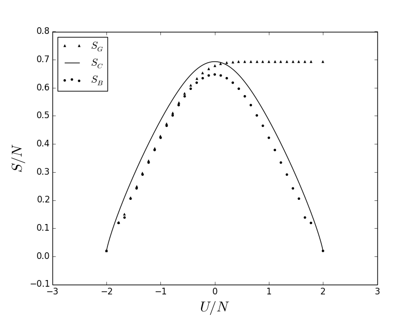
It can be seen that the solid curve representing the canonical entropy lies above for all energies except the highest and lowest, for which they both take on the expected value of . While is also below for negative energies, it continues to rise for positive energies. goes to the value at the highest energy, rather than the value of that would correspond to the two-fold degeneracy of the highest energy level. The negative slope of and for positive energies is consistent with this model exhibiting negative temperatures, but predicts only positive temperatures.
The expressions for the entropy seen in Fig. 1 for the Ising model are qualitatively the same as those seen in Fig. 1 of Ref. [34] for independent two-level objects. Equilibrium between two Ising models of different sizes would also have the same behavior as that shown in Fig. 2 of Ref. [34], which demonstrated that cannot predict the equipartition of energy correctly. The reason is again due to the size dependence of for positive energies. For a given positive energy per spin, the larger system would have a larger value of , so that the smaller system would need more energy to match it. Since this would violate equipartition of energy, the predictions of are incorrect.
III.2 Quantum simple harmonic oscillators
In Ref. [34], exact results were obtained for quantum simple harmonic oscillators, for which and are both defined on a discrete set of energies. They both lie below the canonical entropy for any finite , with above . In the limit , both and are defined for continuous energies and agree with the canonical entropy. Although the system is obviously extensive because it is composed of identical, independent components, neither nor is exactly extensive for finite systems. The canonical entropy, , is extensive. We refer to Ref. [34] for a plot of the behavior.
IV First-order phase transitions
In this section, we analyze first-order phase transitions for various conditions. We start with the first-order phase transition of the twelve-state Potts model, which has short-range interactions. Then we show that the thermodynamic limit obscures the physics of this transition by hiding the terms responsible for it. We then analyze the behavior of systems with long-range interactions, showing that it is essentially the same, even though the appearance of the Boltzmann entropy per site in the thermodynamic limit is quite different.
IV.1 The twelve-state Potts model
The two-dimensional Potts model with states is known to exhibit a first-order phase transition. The Hamiltonian of the model can be written as
| (11) |
where is the Kronecker delta, and the sum is over nearest-neighbor pairs of sites. We simulated the model with the Wang-Landau algorithm to obtain estimates of the density of states [43]. The results of the simulation are shown in Fig. 2 for both the Boltzmann entropy and the canonical entropy . As for models discussed above, lies above for all energies except the ground state energy, for which they both have the value , and for the maximum energy, where they also agree.
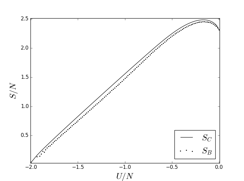
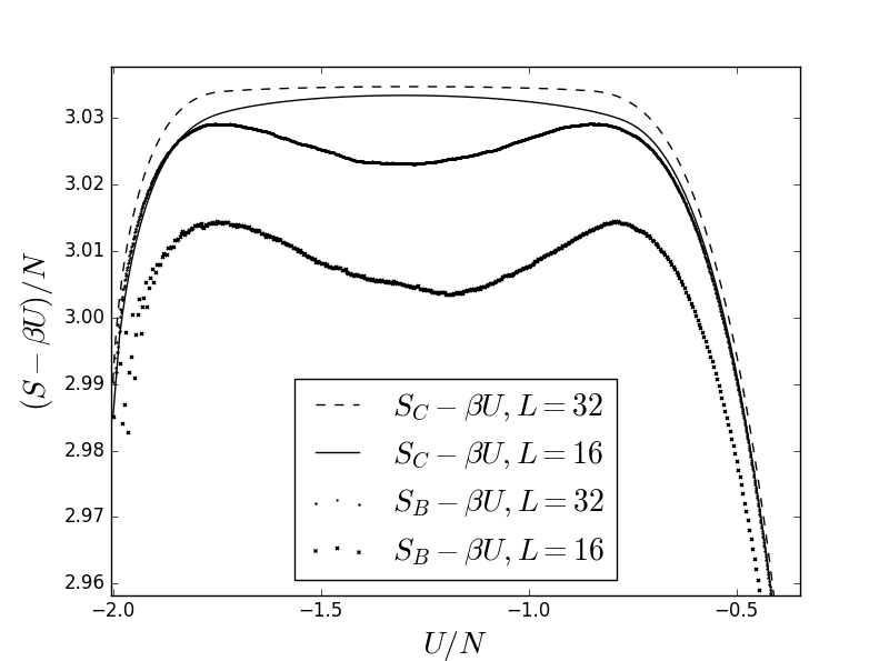
Since the details of the first-order transition are difficult to see in Fig. 2, we have replotted the data differently in Fig. 3 for lattices, with and . This plot shows for both and . The dip in with positive curvature contrasts with , which has negative curvature everywhere, as required by thermodynamic stability. The flattening of the curve for is just visible between and . Note that because of the negative curvature of , a double-tangent construction would not produce the correct entropy for any finite .
IV.2 First-order transitions and the approximation of an infinite system
Examining Fig. 3, we see that the difference between and is smaller for the data than it is for . This is a general property of first-order transitions in systems with short-range interactions, when the entropy is divided by . The coexistence states are suppressed by the boundary energy between the two phases. If is the linear dimension of the system, then the interfacial free energy scales as or , where is the dimension. In terms of the entropy per site, these terms are of order , so that when the entropy per site is calculated for an infinite system, their (apparent) contribution disappears. The usual representation of the thermodynamic limit gives the impression is that the entropy contribution of these coexistence states has vanished[35, 36, 37, 38].
However, the effects of the interfacial terms do not vanish. The coexistence states are suppressed by interfacial energy terms that diverge as (or for this model). As a result, the Boltzmann entropy is not concave in the coexistence region for any finite system, which violates a stability criterion. That violation becomes infinitely strong in an infinite system. If this system is put into thermal contact with any other system, it will leave the eigenstate for a distribution with a much higher probability.
As Fig. 4 shows, the actual behavior of the entropy for large systems is complicated. Outside the region of the first-order transition, scales as . Since the data is plotted as vs. , the curves for , , and agree outside the first-order region.
In the first-order region, is expected to scale as , which is the length of the interface between the ordered and disordered phases. The data is consistent with that behavior, but is still far from the asymptotic region. A plot of vs. for very large should show curves that go to zero (as ) outside the first-order region, but go to a non-zero function in the thermodynamic limit inside the first-order region.
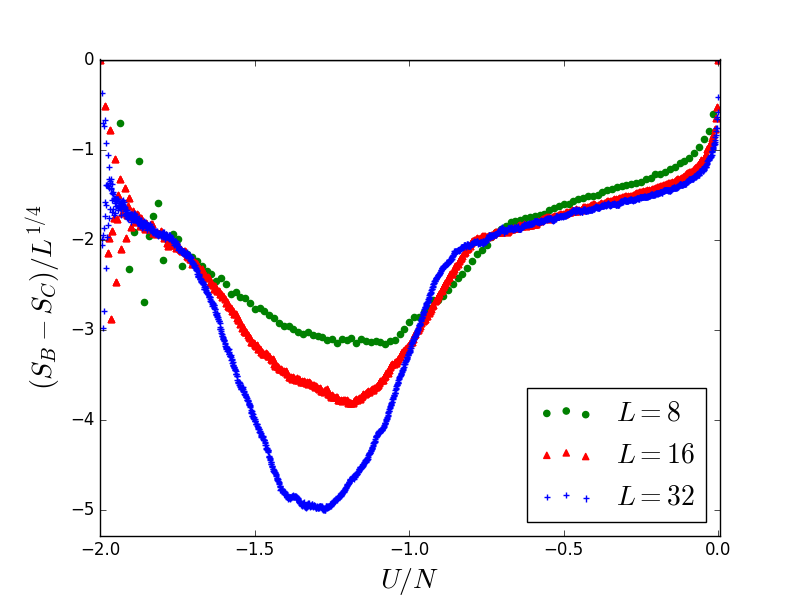
This is not the usual way of representing the thermodynamic limit, but it does display the information about the entropy. A similar plot would exhibit the non-extensive part of the entropy in a gas in a container with walls that adsorbed particles, as mentioned in the introduction.
For a system with long-range interactions, the “interface” between the two phases is of the same dimension as the system, making the interfacial terms go as instead of . This makes no essential difference in the behavior of the first-order transition, but it seems to make a difference because it affects the entropy per site (or per particle) for an infinite system (thermodynamic limit). For long-range interactions, the contributions of the interface that cause the first-order transition do not vanish in the usual representation of the thermodynamic limit.
Because of the different appearance of the first-order transition in the presence of long-range interactions for an infinite system, we give an explicit analysis of a generic quantum model in the next subsection. However, it is important to remember that a first-order transition behaves in essentially the same way, with or without long-range interactions – only its representation is different. As we will show, the thermodynamic entropy is qualitatively the same in both cases.
IV.3 A generic model with long-range interactions and a first-order transition
We now introduce a Gaussian dip in the density of states of a generic quantum model to produce a first-order phase transition. Our model density of states is
| (12) | |||||
The center of the Gaussian term is taken to be
| (13) |
and the width of the Gaussian is
| (14) |
For our examples, we take , , , , , and , but other values give similar results.
The partition function is given by
| (15) |
and the thermodynamic energy is
| (16) |
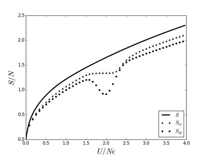
Fig. 5 shows , , and as functions of the energy for . The dip in the density of states is reflected in , which is the logarithm of . A modified dip is also seen in ; the first derivative is non-negative, but the second derivative has a positive region. The canonical entropy shows no dip. It has a negative second derivative at all points, as required by thermodynamic stability.
The development of the first-order transition can be seen in Fig. 6. This plot shows a discontinuity forming in the thermodynamic energy as a function of temperature for , and .
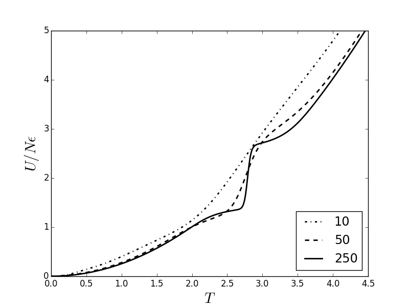
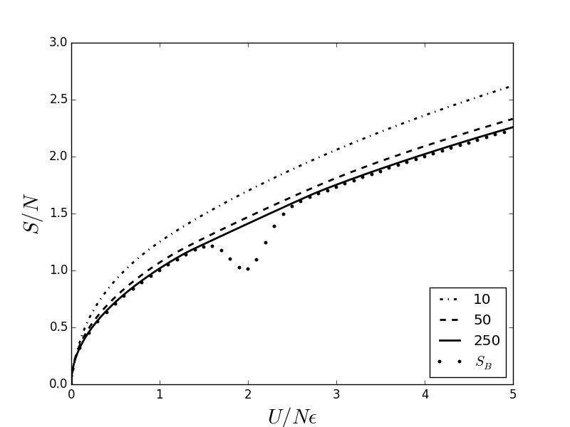
Fig. 7 shows a scaled plot of the canonical entropy as a function of energy for and . Values of are only shown for , but for other values of also follow the curve given in Eq. (12). The dip in (and ) due to the second term in Eq. (12) for remains for all , creating a region with a positive second derivative with respect to . Stability requires that the entropy must have a non-positive second derivative for all and all energies, even for long-range interactions. In the limit , the canonical entropy develops a straight region that corresponds to the first-order transition, just as it does in the case of short-ranged interactions.
V Classical models
There are several classical models with continuous densities of states that provide interesting examples for comparisons between the canonical entropy and the microcanonical entropies and . We begin with a simple power-law density of states to demonstrate the method. We then compare the definitions for a more complicated model suggested by Hilbert, Hänggi, and Dunkel[15]. To clarify the features of the model, we consider three cases for which we can obtain analytic results: an oscillating density of states, and both an exponentially increasing and a decreasing density of states. All models in this section have densities of states defined only for non-negative values of the energy.
V.1 A power-law density of states
A simple classical model density of states is given by a power law.
| (17) |
The partition function for Eq. (17) is found by integration of to be
| (18) |
and the thermodynamic energy is
| (19) |
Note that a system of simple harmonic oscillators with frequency has a power-law density of states with . Its partition function is , with . A classical ideal gas also has a density of states of this form, with and an appropriate choice of .
The canonical entropy is then
| (20) |
where
| (21) |
Note that as , , and , which is a general classical result. Naturally, this behavior violates the third law of thermodynamics, which is only true for quantum systems.
The corresponding expressions for the microcanonical entropies are
| (22) |
where is a constant with units of energy, and
| (23) |
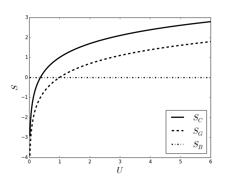
In the limit of large , the three expressions for the entropy agree. For small values of , the expressions for and differ only by a constant, which has no significance in classical statistical mechanics. The differences with are greatest for , which can be seen from Fig. 8. which shows plots of all three expressions for entropy. The Boltzmann entropy is wrong in this extreme case, since it is simply a constant, but it is correct for large values of .
V.2 The Hilbert, Hänggi, and Dunkel model
Hilbert, Hänggi, and Dunkel (HHD) have introduced an interesting model density of states in Ref. [15]. In their Eq. (23), they gave the integral of their density of states as
| (24) |
The density of states itself can be found from the derivative
| (25) |
and the explicit form for is
| (26) | |||||
There is a problem with the form of in Eq. (24) because , although the limit should equal zero. The expression for consistent with is
| (27) |
Nevertheless, we performed our calculations with Eqs. (24) and (26) to facilitate comparison with Ref. [15].
Fig. 9 shows , which is computed numerically, , and for the HHD model. The curves for and agree with those given in Fig. 1.b of Ref. [15]. has an infinite sequence of oscillations, with exponentially increasing magnitude. Due to Eq. (25), the minima in correspond to minima in the slope of . In contrast, the plot of vs. is remarkably smooth, with none of the oscillations that appear in and . As , we again see that , which is typical for the entropy of a classical system. Neither nor exhibits this classical divergence, although the corrected version of in Eq. (27) would show this divergence.
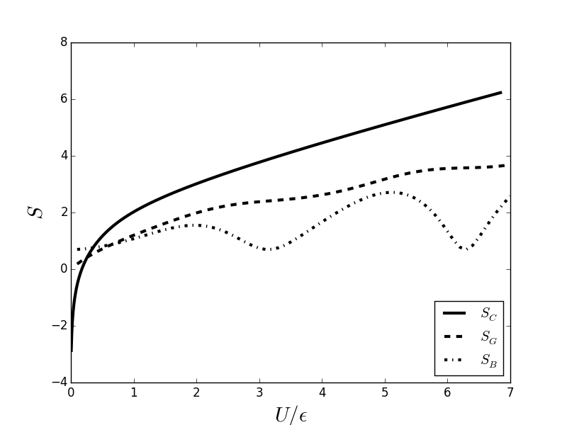
For large values of the energy , the slope of goes to a constant, which is the inverse of the maximum temperature of the model. The unusual phenomenon of a maximum temperature is due to the exponentially increasing part of Eq. (24). The energy dependence of the canonical temperature is shown as a function of the energy in Fig. 10. To see how a maximum temperature arises, we investigate a simpler model with an exponentially increasing density of states below in Subsection V.4.
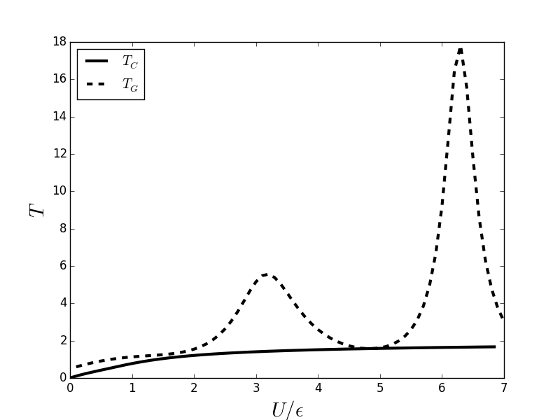
Fig. 10 also shows the Gibbs temperature , and is consistent with Fig. 1.c of Ref. [15]. Since
| (28) |
Fig. 10 shows a peak in corresponding to each minimum of . These peaks in mean that a given value of the temperature corresponds to a sequence of values of . This has been noted by HHD, who regard it as correct thermodynamic behavior, writing that, “the same temperature value or can correspond to vastly different energy values [15].”
We believe that a multiplicity of thermodynamic energies for a single temperature is non-physical. In support of this position, there is a physically reasonable one-to-one relationship between the canonical temperature and the energy .
The sequence of peaks in as a function of is investigated below in Subsection V.3 for a simpler model with a density of states that oscillates, but does not diverge exponentially for large energies.
V.3 An oscillating density of states
To investigate the predicted sequence of peaks in as a function of , discussed in Subsection V.2, we introduce a simpler model with an oscillating density of states, for which the canonical entropy that can be obtained analytically.
| (29) |
The Boltzmann and Gibbs entropies are then
| (30) |
and
| (31) |
The partition function is
| (32) |
the energy is
| (33) | |||||
and the canonical entropy is given by . The expression for the canonical entropy of this model is rather long, but it easy to plot, and Fig. 11 shows , , and . The oscillations in are reflected in oscillations of the slope in . However, oscillations are entirely missing in the canonical entropy.
and show the typical low temperature behavior of classical systems: when , , and . As usual, does not have this feature.
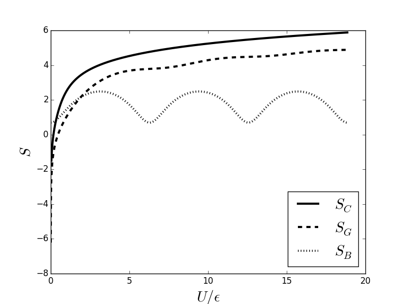
The predictions of and for the behavior of the temperature are similar to those for the HHD model discussed in Subsection V.2. The inverse temperature is the derivative of with respect to . We have not plotted vs. , but it can be seen from Fig. 11 that oscillates between positive and negative slopes, with the slope vanishing at every maximum and minimum, so that at these points.
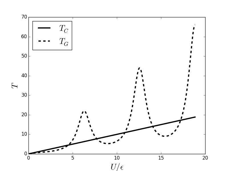
The behavior of as a function of is shown in Fig. 12, which shows a sequence of peaks corresponding to the minima in the slope of in Fig. 11. This behavior is qualitatively the same as that seen in Fig. 10 (Subsection V.2), and again has the consequence that a given value of either or might correspond to many values of the energy .
V.4 An increasing exponential density of states
An exponentially increasing density of states is another simplified version of the HHD model discussed in Subsection V.2. The simplified model is
| (34) |
with .
The partition function is
| (35) |
and the energy is
| (36) |
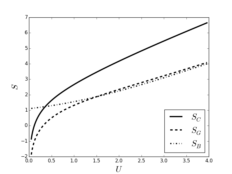
Note that the partition function and the energy both diverge at , or . A peculiarity of this model, which it shares with the HHD model (Subsection V.2), is that there is a maximum temperature, and as .
The canonical entropy for the exponential density of states as a function of is given by
| (37) | |||||
The corresponding expressions for and are
| (38) |
and
| (39) |
All three expressions for entropy are plotted in Fig. 13 as functions of the energy. Because the density of states increases so rapidly, all three expressions agree for large , except for an additive constant that has no significance for classical statistical mechanics. The slope of all three functions goes to the expected value of for large . Both and show the correct divergence to as , but goes to a constant.
V.5 An exponentially decreasing density of states
The case of an exponentially decreasing density of states turns out to be unexpectedly interesting. We write
| (40) |
where we have indicated the negative argument of the exponential function explicitly to avoid confusion.
To calculate the canonical entropy, we find that the partition function is
| (41) |
the energy is
| (42) |
so that the two are related by
| (43) |
Note that and diverge at , but are well defined for all temperatures algebraically greater than .
The canonical entropy as a function of is
| (44) |
The expressions for and are
| (45) |
and
| (46) |
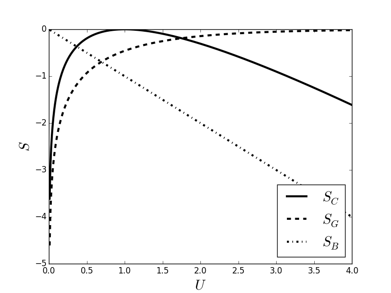
Fig. 14 shows plots of , , and as functions of the energy . and contradict each other, with having a constant negative slope (implying the same negative temperature for all energies, while has a positive slope and positive temperatures for all energies. differs from both, and we regard its predictions as correct.
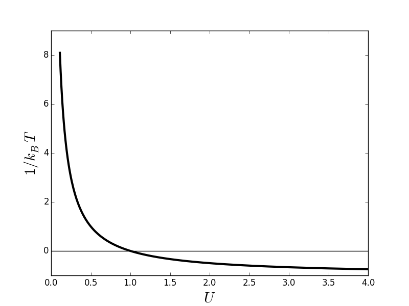
The maximum in the canonical entropy as a function of is somewhat surprising since the density of states is monotonically decreasing. This maximum has the consequence that the energy is finite for infinite temperature: when , and . The canonical temperature is positive for and negative for , as shown in Fig. 15. Such behavior is well-known for models with a maximum in the density of states, like the Ising model. However, the density of states for this model is monotonically decreasing.
VI Conclusions
We have shown that the three proposed definitions give very different expressions for the thermodynamic entropy for various models. Since the thermodynamic entropy must be unique[1], only one of these definitions of the entropy can be correct.
For the models we have investigated, the canonical entropy, , gives physically reasonable predictions for all thermodynamic properties. By construction, these predictions are identical to those of the canonical ensemble, making entropy consistent with Helmholtz free energy and all other thermodynamic potentials.
For all quantum models discussed in Sections III and IV, neither nor gives the correct entropy for any finite system, because they are defined only on a discrete set of energy values. Only in the limit , and become continuous functions of . becomes quantitatively correct for the models discussed in Section III. also agrees for values of the energy corresponding to an increasing density of states, but not for the decreasing density of states for positive energies in the independent-spin model discussed in Ref. [34], or in the Ising model, shown in Fig. 1. It is perhaps significant that no evidence has been published to indicate that should be correct for a decreasing density of states.
In Section IV, both and are seen to disagree with the canonical entropy of the twelve-state Potts model for all system sizes. They both exhibit a range of energies for which their curvature is positive, which violates a condition of thermodynamic stability. If a system in an eigenstate in this region is brought into thermal contact with an exact copy of itself, both systems will go to a new thermodynamic state, and the equilibrium will be described by the canonical entropy.
In Fig. 4, we have suggested a new way of representing in the thermodynamic limit, for a system that exhibits a first-order transition. The quantity does not vanish for in the region of a first-order phase transition, so that the Bolzmann entropy and the canonical entropy should not be regarded as equivalent.
The Gibbs and Boltzmann entropies for the generic density of states for a model with long-range interactions and a first-order phase transition are also incorrect, in that they both contain a region with a positive curvature, even in the limit . The canonical entropy shows no such anomaly.
Our analysis has shown that care must be taken when using the approximation of an infinite system (thermodynamic limit) for first-order transitions. When properly viewed, first-order transitions are all essentially the same, whether the forces are long-range or short-range.
For the classical (continuous) densities of states discussed in Section V, and only give good predictions for the power law density of states for large values of . The Gibbs entropy correctly shows the classical divergence of for for all classical models except the HHD model discussed in Subsection V.2. is essentially correct for the constant density of states discussed in Subsection V.1, and the exponentially increasing density of states discussed in Subsection V.4.
Neither nor shows the correct behavior for the oscillating density of states in Subsections V.2 and V.3. The prediction of peaks in a plot of temperature as a function of energy is a serious departure from physically reasonable behavior.
The case of a decreasing exponential density of states, discussed in Subsection V.5, is particularly interesting in that the three definitions of entropy give completely different predictions for the thermodynamic behavior. We regard the canonical prediction of both positive and negative temperature regions as correct, with high energies corresponding to the most negative temperatures. This confirms the interpretation that negative temperatures are hotter than infinite temperature.
In summary, the canonical entropy provides a correct procedure for calculating the thermodynamic entropy as a function of the energy for both quantum and classical systems from the principles of statistical mechanics. Although the microcanonical definitions of entropy, and , might give reasonable approximations that are useful for a limited class of models, they are not always correct, and their predictions can be misleading.
Acknowledgement
RHS would like to thank Jian-Sheng Wang and Oliver Penrose for their valuable comments, and Roberta Klatzky for many helpful discussions. This research did not receive any specific grant from funding agencies in the public, commercial, or not-for-profit sectors.
References
- Lieb and Yngvason [1997] E. H. Lieb and J. Yngvason, “A guide to entropy and the second law of thermodynamics,” Notices of the AMS, 45 (1997).
- Boltzmann [1877] L. Boltzmann, “Über die Beziehung zwischen dem zweiten Hauptsatze der mechanischen Wärmetheorie und der Wahrscheinlichkeitsrechnung respektive den Sätzen über das Wärmegleichgewicht,” Wien. Ber., 76, 373–435 (1877), reprinted in Wissenschaftliche Abhandlungen von Ludwig Boltzmann (Chelsea, New York Vol. II, pp. 164-223.
- Sharp and Matschinsky [2015] K. Sharp and F. Matschinsky, “Translation of Ludwig Boltzmann’s paper on the relationship between the second fundamental theorem of the mechanical theory of heat and probability calculations regarding the conditions for thermal equilibrium, Sitzungberichte der Kaiserlichen Akademie der Wissenschaften. Mathematisch-Naturwissen Classe. abt. ii, lxxvi 1877, pp 373-435 (Wien. Ber. 1877, 76:373-435). reprinted in Wiss. Abhandlungen, vol. ii, reprint 42, p. 164-223, Barth, Leipzig, 1909,” Entropy, 17, 1971–2009 (2015), ISSN 1099-4300.
- [4] Boltzmann derived the expression for the entropy for classical systems under the assumption that equilibrium corresponded to the maximum of the probability for two systems in equilibrium. The quantum version is due to Planck[5]. Planck is also responsible for the form of the entropy carved into Boltzmann’s grave stone, (where “W” stands for the German word “Wahrscheinlichkeit”, or probability), and the introduction of as the Boltzmann constant.
- Planck [1901] M. Planck, “Über das Gesetz der Energieverteilung im Normalspektrum,” Drudes Annalen, 553, 65–74 (1901), reprinted in Ostwalds Klassiker der exakten Wissenschaften, Band 206, “Die Ableitung der Strahlungsgesteze”.
- Planck [1906] M. Planck, Theorie der Wärmestrahlung (J. A. Barth, Leipzig, 1906) translated into English by Morton Masius in M. Planck, The Theory of Heat Radiation, (Dover, New York, 1991).
- Gibbs [1902] J. W. Gibbs, Elementary Principles of Statistical Mechanics (Yale University Press, New Haven, 1902) reprinted by Dover, New York, 1960.
- [8] We are using the term “Gibbs entropy” to refer to the definition of the entropy in terms of the logarithm of the volume of phase space with energy less than a given energy. The quantum version refers to the sum of all degeneracies of eigenstates with energies below a given energy. It is not to be confused with another definition of entropy due to Gibbs in terms of an integral of , where is the probability of a microscopic state.
- Purcell and Pound [1951] E. M. Purcell and R. V. Pound, “A nuclear spin system at negative temperature,” Phys. Rev., 81, 279–280 (1951).
- Ramsey [1956] N. F. Ramsey, “Thermodynamics and statistical mechanics at negative absolute temperatures,” Phys. Rev., 103, 20–28 (1956).
- Landsberg [1959] P. T. Landsberg, “Negative temperatures,” Phys Rev., 115, 518–520 (1959).
- Dunkel and Hilbert [2006] J. Dunkel and S. Hilbert, “Phase transitions in small systems: Microcanonical vs. canonical ensembles,” Physica A, 370, 390–406 (2006).
- Romero-Rochin [2013] V. Romero-Rochin, “Nonexistence of equilibrium states at absolute negative temperatures,” Phys. Rev. E, 88, 022144 (2013).
- Dunkel and Hilbert [2014] J. Dunkel and S. Hilbert, “Consistent thermostatistics forbids negative absolute temperatures,” Nature Physics, 10, 67–72 (2014).
- Hilbert et al. [2014] S. Hilbert, P. Hänggi, and J. Dunkel, “Thermodynamic laws in isolated systems,” Phys. Rev. E, 90, 062116 (2014).
- Campisi [2015] M. Campisi, “Construction of microcanonical entropy on thermodynamic pillars,” Phys. Rev. E, 91, 052147 (2015).
- Hänggi et al. [2016] P. Hänggi, S. Hilbert, and J. Dunkel, “Meaning of temperature in different thermostatistical ensembles,” Phil. Trans. Roy. Soc. A, 374, 20150039 (2016).
- Sokolov [2014] I. M. Sokolov, “Not hotter than hot,” Nature Physics, 10, 7–8 (2014).
- Swendsen [2002] R. H. Swendsen, “Statistical mechanics of classical systems with distinguishable particles,” J. Stat. Phys., 107, 1143–1165 (2002).
- Swendsen [2006] R. H. Swendsen, “Statistical mechanics of colloids and Boltzmann’s definition of the entropy,” Am. J. Phys., 74, 187–190 (2006).
- Swendsen [2008] R. H. Swendsen, “Gibbs’ paradox and the definition of entropy,” Entropy, 10, 15–18 (2008).
- Swendsen [2011] R. H. Swendsen, “How physicists disagree on the meaning of entropy,” Am. J. Phys., 79, 342–348 (2011).
- Swendsen [2012] R. H. Swendsen, “Choosing a definition of entropy that works,” Found. of Physics, 42, 582–593 (2012a).
- Swendsen [2014] R. H. Swendsen, “Unnormalized probability: A different view of statistical mechanics,” Am. J. Phys., 82, 941–946 (2014).
- Vilar and Rubi [2014] J. M. G. Vilar and J. M. Rubi, “Communication: System-size scaling of Boltzmann and alternate Gibbs entropies,” J. Chem. Phys., 140, 201101 (2014).
- Schneider et al. [2014] U. Schneider, S. Mandt, A. Rapp, S. Braun, H. Weimer, I. Bloch, and A. Rosch, “Comment on ‘Consistent thermostatistics forbids negative absolute temperatures’,” (2014), arXiv:1407.4127v1 [cond-mat.quant-gas].
- Frenkel and Warren [2015] D. Frenkel and P. B. Warren, “Gibbs, Boltzmann, and negative temperatures,” Am. J. Phys., 83, 163–170 (2015).
- Dunkel and Hilbert [2104] J. Dunkel and S. Hilbert, “Reply to Frenkel and Warren [arxiv:1403.4299v1],” (2104), arXiv:1403.6058v1.
- Swendsen and Wang [2015] R. H. Swendsen and J.-S. Wang, “The Gibbs volume entropy is incorrect,” Phys. Rev. E,, 92, 020103(R) (2015).
- Swendsen and Wang [2016] R. H. Swendsen and J.-S. Wang, “Negative temperatures and the definition of entropy,” Physica A, 453, 24 34 (2016).
- Anghel [2015] D.-V. Anghel, “The stumbling block of the Gibbs entropy: the reality of the negative absolute temperatures,” (2015), arXiv:1509.08020v1 [cond-mat,stat-mech].
- Cerino et al. [2015] L. Cerino, A. Puglisi, and A. Vulpiani, “Consistent description of fluctuations requires negative temperatures,” (2015), arXiv:1509.07369v1 [cond-mat,stat-mech].
- Poulter [2015] J. Poulter, “In defence of negative temperature,” (2015), arXiv:1508.00350v2 [cond-mat,stat-mech].
- Swendsen [2015] R. H. Swendsen, “Continuity of the entropy of macroscopic quantum systems,” Phys. Rev. E, 92, 052110 (2015).
- Touchette et al. [2004] H. Touchette, R. S. Ellis, and B. Turkington, “An introduction to the thermodynamic and macrostate levels of nonequivalent ensembles,” Physica A, 340, 138–146 (2004).
- Costeniuc et al. [2006] M. Costeniuc, E. Richard S., and H. Touchette, “Nonconcave entropies from generalized canonical ensembles,” Phys. Rev. E, 74, 010105 (2006).
- Touchette [2011] H. Touchette, “Ensemble equivalence for general many-body systems,” EPL, 96, 50010 (2011).
- Touchette [2015] H. Touchette, “General equivalence and nonequivalence of ensembles: Thermodynamic, macrostate, and measure levels,” J. Stat. Phys., 159, 987 (2015).
- Jin et al. [2013] F. Jin, K. Michielsen, M. A. Novotny, S. Miyashita, S. Yuan, and H. De Raedt, “Quantum decoherence scaling with bath size: Importance of dynamics, connectivity, and randomness,” Phys. Rev. A, 87, 022117 (2013a).
- Jin et al. [2013] F. Jin, T. Neuhaus, K. Michielsen, S. Miyashita, M. A. Novotny, M. I. Katsnelson, and H. De Raedt, “Equilibration and thermalization of classical systems,” New Journal of Physics, 15, 033009 (2013b).
- Novotny et al. [2015] M.A. Novotny, F. Jin, S. Yuan, S. Miyashita, H. De Raedt, and K. Michielsen, “Quantum decoherence at finite temperatures,” (2015), arXiv:1502.03996v1 [cond-mat,stat-mech].
- Novotny et al. [2016] M. A. Novotny, F. Jin, S. Yuan, S. Miyashita, H. De Raedt, and K. Michielsen, “Quantum decoherence and thermalization at finite temperature within the canonical thermal state ensemble,” (2016), arXiv:1601.04209.
- Wang and Landau [2001] F. Wang and D. P. Landau, “Efficient, multiple-range random walk algorithm to calculate the density of states,” Phys. Rev. Lett., 86, 2050–2053 (2001).
- Callen [1985] H. B. Callen, Thermodynamics and an Introduction to Thermostatistics, 2nd ed. (Wiley, New York, 1985).
- Swendsen [2012] R. H. Swendsen, An Introduction to Statistical Mechanics and Thermodynamics (Oxford, London, 2012).
- Beale [1996] P. D. Beale, “Exact distribution of energies in the two-dimensional Ising model,” Phys. Rev. Lett., 76, 78–81 (1996).