Many particle approximation of the Aw-Rascle-Zhang second order model for vehicular traffic

Abstract.

We consider the follow-the-leader approximation of the Aw-Rascle-Zhang (ARZ) model for traffic flow in a multi population formulation. We prove rigorous convergence to weak solutions of the ARZ system in the many particle limit in presence of vacuum. The result is based on uniform 𝐁𝐕𝐁𝐕{\mathbf{BV}} estimates on the discrete particle velocity. We complement our result with numerical simulations of the particle method compared with some exact solutions to the Riemann problem of the ARZ system.

Key words and phrases:
Aw-Rascle-Zhang model, second order models for vehicular traffics, many particle limit.
1991 Mathematics Subject Classification:
Primary: 35L65, 90B20.
MDF is supported by the Italian MIUR-PRIN project 2012L5WXHJ_0032012𝐿5𝑊𝑋𝐻𝐽_0032012L5WXHJ\_003. SF is partially supported by the Italian INdAM-GNAMPA 2015 mini-project: Analisi e stabilità per modelli di equazioni alle derivate parziali nella matematica applicata. MDR is also partially supported by ICM Interdyscyplinarne Centrum Modelowania Matematycznego i Komputerowego, Uniwersytet Warszawski. The authors would like to thanks Giovanni Russo for comments and suggestions on the numerical part.
Corresponding author: M. D. Rosini

Marco Di Francesco and Simone Fagioli

DISIM, Università degli Studi dell’Aquila,

via Vetoio 1 (Coppito), 67100 L’Aquila (AQ), Italy

Massimiliano D. Rosini

Instytut Matematyki, Uniwersytet Marii Curie-Skłodowskiej,

pl. Marii Curie-Skłodowskiej 1, 20-031 Lublin, Poland

1. Introduction

The Aw, Rascle [4] and Zhang [21] (ARZ) model is a second order system describing vehicular traffic. In its continuum formulation, it can be written as the 2×2222\times 2 system of conservation laws in one space dimension

(1) {ρt+(ρv)x=0,t>0,x,[ρ(v+p(ρ))]t+[ρv(v+p(ρ))]x=0,t>0,x.casessubscript𝜌𝑡subscript𝜌𝑣𝑥0formulae-sequence𝑡0𝑥subscriptdelimited-[]𝜌𝑣𝑝𝜌𝑡subscriptdelimited-[]𝜌𝑣𝑣𝑝𝜌𝑥0formulae-sequence𝑡0𝑥\begin{cases}\rho_{t}+\left(\rho\,v\right)_{x}=0,&t>0,~{}x\in{\mathbb{R}},\\ \left[\rho\,(v+p(\rho))\right]_{t}+\left[\rho\,v\,(v+p(\rho))\right]_{x}=0,&t>0,~{}x\in{\mathbb{R}}.\end{cases}

The conserved variables ρ𝜌\rho and [ρ(v+p(ρ))]delimited-[]𝜌𝑣𝑝𝜌[\rho\,(v+p(\rho))] describe respectively the density and the generalized momentum of the system. v𝑣v is the velocity. The quantity

wv+p(ρ)approaches-limit𝑤𝑣𝑝𝜌w\doteq v+p(\rho)

is called Lagrangian marker. The function p𝑝p in (1) is the pressure function and accounts for drivers’ reactions to the state of traffic in front of them. While traffic flow is one of the main motivating applications behind the system (1), we see a growing interest nowadays on different contexts as crowd dynamics and bio-mathematics.

The instability near the vacuum state makes the mathematical theory for (1) a challenging topic. For this reason, as in [2, 1, 15], we study (1) in the Riemann invariant coordinates (v,w)𝑣𝑤(v,w) and use the following expressions for the density

ρp1(wv).approaches-limit𝜌superscript𝑝1𝑤𝑣\displaystyle\rho\doteq p^{-1}(w-v).

It is well known since [3] and the earlier works [14, 18] (see also a related result in [17]) that the discrete Lagrangian counterpart of (1) is provided by the second order follow-the-leader system

(2) {x˙i=Vi,V˙i=p(1xi+1xi)Vi+1Vi(xi+1xi)2,casessubscript˙𝑥𝑖subscript𝑉𝑖otherwisesubscript˙𝑉𝑖superscript𝑝1subscript𝑥𝑖1subscript𝑥𝑖subscript𝑉𝑖1subscript𝑉𝑖superscriptsubscript𝑥𝑖1subscript𝑥𝑖2otherwise\begin{cases}\displaystyle{\dot{x}_{i}=V_{i}}\,,&\\ \displaystyle{\dot{V}_{i}=p^{\prime}\left(\frac{1}{x_{i+1}-x_{i}}\right)\frac{V_{i+1}-V_{i}}{(x_{i+1}-x_{i})^{2}}}\,,&\end{cases}

where xi(t)subscript𝑥𝑖𝑡x_{i}(t) and Vi(t)subscript𝑉𝑖𝑡V_{i}(t) are location of the tail and speed of the i𝑖i-th vehicle at time t𝑡t. In terms of the discrete Lagrangian marker

wiVi+p(1xi+1xi),approaches-limitsubscript𝑤𝑖subscript𝑉𝑖𝑝1subscript𝑥𝑖1subscript𝑥𝑖w_{i}\doteq V_{i}+p\left(\frac{1}{x_{i+1}-x_{i}}\right),

the system (2) reads in the simpler form

(3) {x˙i=wip(1xi+1xi),w˙i=0.casessubscript˙𝑥𝑖subscript𝑤𝑖𝑝1subscript𝑥𝑖1subscript𝑥𝑖otherwisesubscript˙𝑤𝑖0otherwise\begin{cases}\displaystyle{\dot{x}_{i}=w_{i}-p\left(\frac{1}{x_{i+1}-x_{i}}\right)},&\\ \displaystyle{\dot{w}_{i}=0}\,.&\end{cases}

The simpler form (3) highlights the fact that the follow-the-leader system (2) describes a particle system with many species. Hence (2) is a microscopic multi population model, in which the i𝑖i-th vehicle has length [1/p1(wi)]delimited-[]1superscript𝑝1subscript𝑤𝑖[1/p^{-1}(w_{i})] and maximal speed wisubscript𝑤𝑖w_{i}, which are constant in time and depend on the initial datum of the Lagrangian marker.

The goal of this paper is to approximate (under reasonable assumptions on p𝑝p) the 2×2222\times 2 system of nonlinear conservation laws (1) with the first order microscopic model (3), that describes a multi population interacting many particle system. The technique we adopt is a slight variation of that introduced in [12], which applies to the approximation of first order LWR models [16, 19] by a (simpler) first order version of the follow-the-leader system. Despite the second order nature of (1), the strategy developed in [12] applies also in this case (see also [9, 10, 11] for other applications of the techniques introduced in [12]). This reveals that the multi-species nature of the ARZ model is quite relevant in the dynamics. Our rigorous results only deal with the convergence toward a weak solution to (1). The problem of the uniqueness of entropy solutions for (1) is quite a hard task, and we do not address it here, see [2, 1]. Our main convergence result is stated in Theorem 5 below.

We also perform numerical simulations that suggest that the solution of the microscopic model (3) converges to a solution of the macroscopic model (1) as the number of particles goes to infinity. In particular, we will make the tests considered in [8] to show that we do not have the spurious oscillations generated, for instance, by the Godunov method near contact discontinuities. We will also make the test considered in [3] to show that our algorithm is able to cope with the vacuum.

Our approach deeply differ from the one proposed in [3]. Indeed, there the authors show how the ARZ model written in Lagrangian mass coordinates can be viewed away from the vacuum as the limit of a time discretization of a second order microscopic model as the number of vehicles increases, with a scaling in space and time (a zoom) for which the density and the velocity remain fixed. On the contrary, we consider the ARZ model written in the Eulerian coordinates, so that the vacuum is a state eventually achieved by the solutions, and we introduce the underlying microscopic model without performing any time discretization.

We recall that the numerical transport-equilibrium scheme proposed in [8] is based on both a (Glimm) random sampling strategy and the Godunov method. As a consequence, this method is non-conservative. Moreover, it cannot be applied in the presence of the vacuum state. On the contrary, our method is conservative and is able to cope with the vacuum. Let us finally underline that the approximate solutions constructed with both methods have sharp (without numerical diffusion) contact discontinuities and show numerical convergence. We remark that the model (1) can be formulated also with a relaxation term with a prescribed equilibrium velocity, see [3]. We shall apply our approach to such an extended version of the ARZ model in a future work.

The present paper is structured as follows. In Section 2 we recall the basic properties of the discrete follow-the-leader model and of the continuum ARZ system. In particular we prove a discrete maximum principle in Lemma 3 which was not present in the literature to our knowledge. In Section 3 we construct the atomization scheme and prove its convergence in the Theorem 5. In Section 4 we perform numerical tests with simple Riemann problems, including cases with vacuum.

2. Preliminaries

In this section we recall basic facts about the ARZ model (1) and the discrete follow-the-leader system (3).

2.1. The ARZ model

Consider the Cauchy problem for the ARZ model (1)

(4) {ρt+(ρv)x=0,t>0,x,(ρw)t+(ρvw)x=0,t>0,x,v(0,x)=v¯(x),x,w(0,x)=w¯(x),x,casessubscript𝜌𝑡subscript𝜌𝑣𝑥0formulae-sequence𝑡0𝑥subscript𝜌𝑤𝑡subscript𝜌𝑣𝑤𝑥0formulae-sequence𝑡0𝑥𝑣0𝑥¯𝑣𝑥𝑥𝑤0𝑥¯𝑤𝑥𝑥\begin{cases}\rho_{t}+\left(\rho\,v\right)_{x}=0,&t>0,~{}x\in{\mathbb{R}},\\ (\rho\,w)_{t}+\left(\rho\,v\,w\right)_{x}=0,&t>0,~{}x\in{\mathbb{R}},\\ v(0,x)=\bar{v}(x),&x\in{\mathbb{R}},\\ w(0,x)=\bar{w}(x),&x\in{\mathbb{R}},\end{cases}

where (v,w)𝑣𝑤(v,w) is the unknown variable and (v¯,w¯)¯𝑣¯𝑤(\bar{v},\bar{w}) is the corresponding initial datum. More precisely, (v,w)𝑣𝑤(v,w) belongs to 𝒲{(v,w)+2:vw}approaches-limit𝒲conditional-set𝑣𝑤superscriptsubscript2𝑣𝑤\mathcal{W}\doteq\left\{(v,w)\in{\mathbb{R}}_{+}^{2}\colon v\leq w\right\} and

ρp1(wv)+approaches-limit𝜌superscript𝑝1𝑤𝑣subscript\rho\doteq p^{-1}(w-v)\in{\mathbb{R}}_{+}

is the corresponding density, where p𝐂𝟎(+;+)𝐂𝟐(]0,+[;+)𝑝superscript𝐂0subscriptsubscriptsuperscript𝐂20subscriptp\in\mathbf{C^{0}}({\mathbb{R}}_{+};{\mathbb{R}}_{+})\cap\mathbf{C^{2}}(\left]0,+\infty\right[;{\mathbb{R}}_{+}) satisfies

(5) p(0+)=0,𝑝superscript00\displaystyle p(0^{+})=0, p(ρ)>0superscript𝑝𝜌0\displaystyle p^{\prime}(\rho)>0 and 2p(ρ)+ρp′′(ρ)>02superscript𝑝𝜌𝜌superscript𝑝′′𝜌0\displaystyle 2\,p^{\prime}(\rho)+\rho\,p^{\prime\prime}(\rho)>0 for every ρ>0.for every 𝜌0\displaystyle\text{for every }\rho>0.
Example 1 (Examples of pressure functions).

In [3] the authors consider

p(ρ){vrefγ[ρρm]γ,γ>0,vreflog[ρρm],γ=0,approaches-limit𝑝𝜌casessubscript𝑣ref𝛾superscriptdelimited-[]𝜌subscript𝜌𝑚𝛾𝛾0subscript𝑣ref𝜌subscript𝜌𝑚𝛾0p(\rho)\doteq\begin{cases}\dfrac{v_{\rm ref}}{\gamma}\left[\dfrac{\rho}{\rho_{m}}\right]^{\gamma},&\gamma>0\,,\\[7.0pt] v_{\rm ref}\,\log\left[\dfrac{\rho}{\rho_{m}}\right],&\gamma=0\,,\end{cases}

where ρm>0subscript𝜌𝑚0\rho_{m}>0 is the maximal density and vref>0subscript𝑣ref0v_{\rm ref}>0 is a reference velocity. The above choice reduces to the original one proposed in [4] when vref/(γρmγ)=1subscript𝑣ref𝛾superscriptsubscript𝜌𝑚𝛾1v_{\rm ref}/(\gamma\,\rho_{m}^{\gamma})=1 and γ>0𝛾0\gamma>0. We also recall that in [6] the authors consider

p(ρ)(1ρ1ρm)γ.approaches-limit𝑝𝜌superscript1𝜌1subscript𝜌𝑚𝛾p(\rho)\doteq\left(\frac{1}{\rho}-\frac{1}{\rho_{m}}\right)^{-\gamma}.

By definition, we have that the vacuum state ρ=0𝜌0\rho=0 corresponds to the half line 𝒲0{(v,w)T𝒲:v=w}approaches-limitsubscript𝒲0conditional-setsuperscript𝑣𝑤𝑇𝒲𝑣𝑤\mathcal{W}_{0}\doteq\left\{(v,w)^{T}\in\mathcal{W}\colon v=w\right\} and the non-vacuum states ρ>0𝜌0\rho>0 to 𝒲0c𝒲𝒲0approaches-limitsuperscriptsubscript𝒲0𝑐𝒲subscript𝒲0\mathcal{W}_{0}^{c}\doteq\mathcal{W}\setminus\mathcal{W}_{0}. As in [2, 1], we consider initial data (v¯,w¯)𝐁𝐕(;𝒲)¯𝑣¯𝑤𝐁𝐕𝒲(\bar{v},\bar{w})\in{\mathbf{BV}}({\mathbb{R}};\mathcal{W}) such that

(6) ((v¯,w¯)(x),(v¯,w¯)(x+))𝔊,¯𝑣¯𝑤superscript𝑥¯𝑣¯𝑤superscript𝑥𝔊\displaystyle((\bar{v},\bar{w})(x^{-}),(\bar{v},\bar{w})(x^{+}))\in\mathfrak{G}, x,𝑥\displaystyle x\in{\mathbb{R}},

where (v¯,w¯)(x)¯𝑣¯𝑤superscript𝑥(\bar{v},\bar{w})(x^{-}) and (v¯,w¯)(x+)¯𝑣¯𝑤superscript𝑥(\bar{v},\bar{w})(x^{+}) denote the traces of (v¯,w¯)¯𝑣¯𝑤(\bar{v},\bar{w}) along a Lipschitz curve of jump (see [20] for a precise formulation of the regularity of 𝐁𝐕𝐁𝐕{\mathbf{BV}} functions) and

𝔊{((v,w),(vr,wr))𝒲2:(v,w)𝒲0(vr,wr)𝒲0}(v,w)=(vr,wr)and(v,w)𝒲0c(vr,wr)𝒲0}(vr,wr)=(w,w)}.\mathfrak{G}\doteq\left\{((v_{\ell},w_{\ell}),(v_{r},w_{r}))\in\mathcal{W}^{2}\colon\begin{array}[]{@{}l@{}}\left.\begin{array}[]{l@{}}(v_{\ell},w_{\ell})\in\mathcal{W}_{0}\\ (v_{r},w_{r})\in\mathcal{W}_{0}\end{array}\right\}\Rightarrow(v_{\ell},w_{\ell})=(v_{r},w_{r})\\ \left.\begin{array}[]{l@{}}\text{and}\end{array}\right.\\ \left.\begin{array}[]{l@{}}(v_{\ell},w_{\ell})\in\mathcal{W}_{0}^{c}\\ (v_{r},w_{r})\in\mathcal{W}_{0}\end{array}\right\}\Rightarrow(v_{r},w_{r})=\left(w_{\ell},w_{\ell}\right)\end{array}\right\}.

The introduction of the condition (6) to select the physically reasonable initial data of (4) in the Riemann invariant coordinates is motivated in [2, Remark 2.1]. We emphasise that such condition is not needed in the proof of our main analytical result. However, (6) is partly motivated by our numerical tests.

Following [2], we use the following definition for weak solutions of (1).

Definition 2 (Weak solutions).

Let (v¯,w¯)𝐋(;𝒲)¯𝑣¯𝑤superscript𝐋𝒲(\bar{v},\bar{w})\in\mathbf{L^{\infty}}({\mathbb{R}};\,\mathcal{W}). We say that a function (v,w)𝐋(+×;𝒲)𝐂𝟎(+;𝐋𝐥𝐨𝐜𝟏(;𝒲))𝑣𝑤superscript𝐋subscript𝒲superscript𝐂0subscriptsuperscriptsubscript𝐋𝐥𝐨𝐜1𝒲(v,w)\in\mathbf{L^{\infty}}({\mathbb{R}}_{+}\times{\mathbb{R}};\,\mathcal{W})\cap\mathbf{C^{0}}({\mathbb{R}}_{+};\,\mathbf{L_{loc}^{1}}({\mathbb{R}};\,\mathcal{W})) is a weak solution of (4) if it satisfies the initial condition (v(0,x),w(0,x))=(v¯(x),w¯(x))𝑣0𝑥𝑤0𝑥¯𝑣𝑥¯𝑤𝑥(v(0,x),w(0,x))=(\bar{v}(x),\bar{w}(x)) for a.e. x𝑥x\in{\mathbb{R}} and for any test function ϕ𝐂𝐜(]0,+[×;)\phi\in\mathbf{C_{c}^{\infty}}(]0,+\infty[\times{\mathbb{R}};\,{\mathbb{R}})

(7) +p1(v,w)(ϕt+vϕx)(1w)dxdt=(00).subscriptsubscriptsubscriptsuperscript𝑝1𝑣𝑤subscriptitalic-ϕ𝑡𝑣subscriptitalic-ϕ𝑥matrix1𝑤differential-d𝑥differential-d𝑡matrix00\int_{{\mathbb{R}}_{+}}\int_{\mathbb{R}}p^{-1}(v,w)\,(\phi_{t}+v\,\phi_{x})\begin{pmatrix}1\\ w\end{pmatrix}\,{\rm{d}}x\,{\rm{d}}t=\begin{pmatrix}0\\ 0\end{pmatrix}.

For the existence of weak solutions to (4) away from the vacuum we refer to [13], see [15] for the existence with vacuum, and [5] for the existence of entropy weak solutions.

Let us briefly recall the main properties of the solutions to (4). If the initial density ρ¯p1(w¯v¯)approaches-limit¯𝜌superscript𝑝1¯𝑤¯𝑣\bar{\rho}\doteq p^{-1}(\bar{w}-\bar{v}) has compact support, then the support of ρ𝜌\rho has finite speed of propagation. The maximum principle holds true in the Riemann invariant coordinates (v,w)𝑣𝑤(v,w), but not in the conserved variables (ρ,ρw)𝜌𝜌𝑤(\rho,\rho\,w) as a consequence of hysteresis processes. Moreover, the total space occupied by the vehicles (if they were packed “nose to tail”) is time independent: ρ(t,x)dx=Mρ¯(x)dxsubscript𝜌𝑡𝑥differential-d𝑥𝑀approaches-limitsubscript¯𝜌𝑥differential-d𝑥\int_{\mathbb{R}}\rho(t,x)\,{\rm{d}}x=M\doteq\int_{\mathbb{R}}\bar{\rho}(x)\,{\rm{d}}x for all t0𝑡0t\geq 0.

We remark that a simple byproduct of our result is an alternative proof of the existence of weak solutions in the sense of Definition 2.

2.2. Follow-the-leader model

Multi population microscopic models of vehicular traffic are typically based on the so called Follow-The-Leader (FTL) model.

Consider [N+1]delimited-[]𝑁1[N+1] ordered particles localised on {\mathbb{R}}. Denote by txi(t)maps-to𝑡subscript𝑥𝑖𝑡t\mapsto x_{i}(t) the position of the i𝑖i-th particle for i=0,,N𝑖0𝑁i=0,\ldots,N. Then, according to the FTL model, the evolution of the particles (which mimics the evolution of the position of [N+1]delimited-[]𝑁1[N+1] vehicles along the road) is described inductively by the following Cauchy problem for a system of ordinary differential equations

(8) {x˙N(t)=wN1,x˙i(t)=vi(1xi+1(t)xi(t)),i=0,,N1,xi(0)=x¯i,i=0,,N,casessubscript˙𝑥𝑁𝑡subscript𝑤𝑁1otherwisesubscript˙𝑥𝑖𝑡subscript𝑣𝑖1subscript𝑥𝑖1𝑡subscript𝑥𝑖𝑡𝑖0𝑁1subscript𝑥𝑖0subscript¯𝑥𝑖𝑖0𝑁\begin{cases}\dot{x}_{N}(t)=w_{N-1},\\ \dot{x}_{i}(t)=v_{i}\left(\dfrac{1}{x_{i+1}(t)-x_{i}(t)}\right),&i=0,\ldots,N-1,\\ x_{i}(0)=\bar{x}_{i},&i=0,\ldots,N,\end{cases}

where

vi(ρ)wip(ρ),approaches-limitsubscript𝑣𝑖𝜌subscript𝑤𝑖𝑝𝜌v_{i}(\rho)\doteq w_{i}-p(\rho),

w0,,wNsubscript𝑤0subscript𝑤𝑁w_{0},\ldots,w_{N} are [N+1]delimited-[]𝑁1[N+1] strictly positive constants, p𝐂𝟐(+;+)𝑝superscript𝐂2subscriptsubscriptp\in\mathbf{C^{2}}({\mathbb{R}}_{+};{\mathbb{R}}_{+}) satisfies (5), and x¯0<<x¯Nsubscript¯𝑥0subscript¯𝑥𝑁\bar{x}_{0}<\ldots<\bar{x}_{N} are the initial positions of the particles. The quantity wi=vi(0)subscript𝑤𝑖subscript𝑣𝑖0w_{i}=v_{i}(0) is the maximum possible velocity allowed for the i𝑖i-th particle. Clearly, only the leading particle xNsubscript𝑥𝑁x_{N} reaches its maximal velocity wNsubscript𝑤𝑁w_{N}, as the vacuum state is achieved only ahead of xNsubscript𝑥𝑁x_{N}.

The quantity Rip1(wi)>0approaches-limitsubscript𝑅𝑖superscript𝑝1subscript𝑤𝑖0R_{i}\doteq p^{-1}(w_{i})>0 is the maximum discrete density of the i𝑖i-th particle, so that Ri1superscriptsubscript𝑅𝑖1R_{i}^{-1} is the length of the i𝑖i-th particle, vi(Ri)=0subscript𝑣𝑖subscript𝑅𝑖0v_{i}(R_{i})=0 and we assume that at time t=0𝑡0t=0

(9) x¯i+1x¯i1Ri,subscript¯𝑥𝑖1subscript¯𝑥𝑖1subscript𝑅𝑖\displaystyle\bar{x}_{i+1}-\bar{x}_{i}\geq\dfrac{1}{R_{i}}, i=0,,N1.𝑖0𝑁1\displaystyle i=0,\ldots,N-1.

System (8) can be solved inductively starting from i=N𝑖𝑁i=N. Indeed, we immediately deduce that

xN(t)=x¯N+wN1t.subscript𝑥𝑁𝑡subscript¯𝑥𝑁subscript𝑤𝑁1𝑡x_{N}(t)=\bar{x}_{N}+w_{N-1}\,t.

Then, we can compute txi(t)maps-to𝑡subscript𝑥𝑖𝑡t\mapsto x_{i}(t) once we know txi+1(t)maps-to𝑡subscript𝑥𝑖1𝑡t\mapsto x_{i+1}(t). In fact, according with the system (8) the velocity of the i𝑖i-th particle depends on its distance from the (i+1)𝑖1(i+1)-th particle alone via the smooth velocity map visubscript𝑣𝑖v_{i}. In order to ensure that the (unique) solution to (8) exists globally in time, we need to prove that the distances [xi+1(t)xi(t)]delimited-[]subscript𝑥𝑖1𝑡subscript𝑥𝑖𝑡[x_{i+1}(t)-x_{i}(t)] never degenerate. This is proven in the next lemma, which extends a similar one in [12] to our multi population system.

Lemma 3 (Discrete maximum principle).

For all i=0,,N1𝑖0𝑁1i=0,\ldots,N-1, we have

1Rixi+1(t)xi(t)x¯Nx¯0+wN1t1subscript𝑅𝑖subscript𝑥𝑖1𝑡subscript𝑥𝑖𝑡subscript¯𝑥𝑁subscript¯𝑥0subscript𝑤𝑁1𝑡\displaystyle\dfrac{1}{R_{i}}\leq x_{i+1}(t)-x_{i}(t)\leq\bar{x}_{N}-\bar{x}_{0}+w_{N-1}\,t for all times t0.for all times 𝑡0\displaystyle\text{for all times }t\geq 0.
Proof.

We first prove the lower bound. At time t=0𝑡0t=0 the lower bound is satisfied because of (9). We shall prove that

(\ast) inft0[xi+1(t)xi(t)]1Ri,subscriptinfimum𝑡0delimited-[]subscript𝑥𝑖1𝑡subscript𝑥𝑖𝑡1subscript𝑅𝑖\displaystyle\inf_{t\geq 0}\left[\vphantom{\vec{V}}x_{i+1}(t)-x_{i}(t)\right]\geq\dfrac{1}{R_{i}}, i=0,,N1,𝑖0𝑁1\displaystyle i=0,\ldots,N-1,

by a recursive argument on i𝑖i. The statement is true for i=N1𝑖𝑁1i=N-1. Indeed, since x˙N1(t)wN1=x˙N(t)subscript˙𝑥𝑁1𝑡subscript𝑤𝑁1subscript˙𝑥𝑁𝑡\dot{x}_{N-1}(t)\leq w_{N-1}=\dot{x}_{N}(t) we have that xN1(t)<xN(t)subscript𝑥𝑁1𝑡subscript𝑥𝑁𝑡x_{N-1}(t)<x_{N}(t) for all t0𝑡0t\geq 0 and

xN(t)xN1(t)=subscript𝑥𝑁𝑡subscript𝑥𝑁1𝑡absent\displaystyle x_{N}(t)-x_{N-1}(t)= x¯Nx¯N1+0t[wN1vN1(1xN(s)xN1(s))]dssubscript¯𝑥𝑁subscript¯𝑥𝑁1superscriptsubscript0𝑡delimited-[]subscript𝑤𝑁1subscript𝑣𝑁11subscript𝑥𝑁𝑠subscript𝑥𝑁1𝑠differential-d𝑠\displaystyle~{}\bar{x}_{N}-\bar{x}_{N-1}+\int_{0}^{t}\left[w_{N-1}-v_{N-1}\left(\dfrac{1}{x_{N}(s)-x_{N-1}(s)}\right)\right]{\rm{d}}s
=\displaystyle= x¯Nx¯N1+0tp(1xN(s)xN1(s))dsx¯Nx¯N11RN1,subscript¯𝑥𝑁subscript¯𝑥𝑁1superscriptsubscript0𝑡𝑝1subscript𝑥𝑁𝑠subscript𝑥𝑁1𝑠differential-d𝑠subscript¯𝑥𝑁subscript¯𝑥𝑁11subscript𝑅𝑁1\displaystyle~{}\bar{x}_{N}-\bar{x}_{N-1}+\int_{0}^{t}p\left(\dfrac{1}{x_{N}(s)-x_{N-1}(s)}\right){\rm{d}}s\geq\bar{x}_{N}-\bar{x}_{N-1}\geq\dfrac{1}{R_{N-1}},

because p(ρ)>0𝑝𝜌0p(\rho)>0 for all ρ>0𝜌0\rho>0. Assume now that

inft0[xi+2(t)xi+1(t)]1Ri+1subscriptinfimum𝑡0delimited-[]subscript𝑥𝑖2𝑡subscript𝑥𝑖1𝑡1subscript𝑅𝑖1\inf_{t\geq 0}\left[\vphantom{\vec{V}}x_{i+2}(t)-x_{i+1}(t)\right]\geq\dfrac{1}{R_{i+1}}

and by contradiction that there exist t2>t10subscript𝑡2subscript𝑡10t_{2}>t_{1}\geq 0 such that

xi+1(t)xi(t)>1Risubscript𝑥𝑖1𝑡subscript𝑥𝑖𝑡1subscript𝑅𝑖\displaystyle x_{i+1}(t)-x_{i}(t)>\dfrac{1}{R_{i}} for all t[0,t1[,for all 𝑡0subscript𝑡1\displaystyle\text{for all }t\in\left[0,t_{1}\right[,
xi+1(t1)xi(t1)=1Ri,subscript𝑥𝑖1subscript𝑡1subscript𝑥𝑖subscript𝑡11subscript𝑅𝑖\displaystyle x_{i+1}(t_{1})-x_{i}(t_{1})=\dfrac{1}{R_{i}},
(\star) 0<xi+1(t)xi(t)<1Ri0subscript𝑥𝑖1𝑡subscript𝑥𝑖𝑡1subscript𝑅𝑖\displaystyle 0<x_{i+1}(t)-x_{i}(t)<\dfrac{1}{R_{i}} for all t]t1,t2].for all 𝑡subscript𝑡1subscript𝑡2\displaystyle\text{for all }t\in\left]t_{1},t_{2}\right].

Since visubscript𝑣𝑖v_{i} is strictly decreasing, for any t]t1,t2]𝑡subscript𝑡1subscript𝑡2t\in\left]t_{1},t_{2}\right] we have that x˙i(t)<vi(Ri)=0=vi+1(Ri+1)x˙i+1(t)subscript˙𝑥𝑖𝑡subscript𝑣𝑖subscript𝑅𝑖0subscript𝑣𝑖1subscript𝑅𝑖1subscript˙𝑥𝑖1𝑡\dot{x}_{i}(t)<v_{i}(R_{i})=0=v_{i+1}(R_{i+1})\leq\dot{x}_{i+1}(t). Consequently, for any t]t1,t2]𝑡subscript𝑡1subscript𝑡2t\in\left]t_{1},t_{2}\right]

xi(t)xi(t1),subscript𝑥𝑖𝑡subscript𝑥𝑖subscript𝑡1\displaystyle x_{i}(t)\leq x_{i}(t_{1}), xi+1(t)xi+1(t1),subscript𝑥𝑖1𝑡subscript𝑥𝑖1subscript𝑡1\displaystyle x_{i+1}(t)\geq x_{i+1}(t_{1}),

and therefore

xi+1(t)xi(t)xi+1(t1)xi(t1)=1Ri,subscript𝑥𝑖1𝑡subscript𝑥𝑖𝑡subscript𝑥𝑖1subscript𝑡1subscript𝑥𝑖subscript𝑡11subscript𝑅𝑖x_{i+1}(t)-x_{i}(t)\geq x_{i+1}(t_{1})-x_{i}(t_{1})=\dfrac{1}{R_{i}},

which contradicts (\star2.2). Hence, (\ast2.2) is satisfied and the lower bound is proven.

Finally, the upper bound easily follows from the lower bound. Indeed, by the first equation of (8) and the lower bound 1[x1(t)x0(t)]R01delimited-[]subscript𝑥1𝑡subscript𝑥0𝑡subscript𝑅01\leq[x_{1}(t)-x_{0}(t)]\,R_{0} just proved, we have that xN(t)=x¯N+wN1tsubscript𝑥𝑁𝑡subscript¯𝑥𝑁subscript𝑤𝑁1𝑡x_{N}(t)=\bar{x}_{N}+w_{N-1}\,t and x0(t)x¯0+v0(R0)t=x¯0subscript𝑥0𝑡subscript¯𝑥0subscript𝑣0subscript𝑅0𝑡subscript¯𝑥0x_{0}(t)\geq\bar{x}_{0}+v_{0}(R_{0})\,t=\bar{x}_{0}. ∎

We emphasise that the above discrete maximum principle is a direct consequence of the transport nature behind the FTL system (8), similarly to what happens in the first order FTL system considered in [12]. Indeed, the global bound for the discrete density is propagated from the last particle xNsubscript𝑥𝑁x_{N} back to all the other particles, as emphasised by the recursive argument in the proof of Lemma 3.

3. The atomization scheme and the strong convergence

We now introduce our atomization scheme for the Cauchy problem (4). Let (v¯,w¯)𝐁𝐕(;𝒲)¯𝑣¯𝑤𝐁𝐕𝒲(\bar{v},\bar{w})\in{\mathbf{BV}}({\mathbb{R}};\mathcal{W}) satisfy (6) and such that ρ¯p1(w¯v¯)approaches-limit¯𝜌superscript𝑝1¯𝑤¯𝑣\bar{\rho}\doteq p^{-1}(\bar{w}-\bar{v}) belongs to 𝐋𝟏(;+)superscript𝐋1subscript\mathbf{L^{1}}({\mathbb{R}};{\mathbb{R}}_{+}) and is compactly supported. Denote by x¯min<x¯maxsubscript¯𝑥subscript¯𝑥\bar{x}_{\min}<\bar{x}_{\max} the extremal points of the convex hull of the compact support of ρ¯¯𝜌\bar{\rho}, namely

[a,b]supp(ρ¯)[a,b]=[x¯min,x¯max].subscriptsupp¯𝜌𝑎𝑏𝑎𝑏subscript¯𝑥subscript¯𝑥\bigcap_{\left[a,b\right]\supseteq{\mathrm{supp}}\left(\bar{\rho}\right)}\left[a,b\right]=\left[\bar{x}_{\min},\bar{x}_{\max}\right].

Fix n𝑛n\in{\mathbb{N}} sufficiently large. Let Mρ¯𝐋𝟏()>0approaches-limit𝑀subscriptnorm¯𝜌superscript𝐋10M\doteq\left\|\bar{\rho}\right\|_{\mathbf{L^{1}}({\mathbb{R}})}>0 and split the subgraph of ρ¯¯𝜌\bar{\rho} in Nn2napproaches-limitsubscript𝑁𝑛superscript2𝑛N_{n}\doteq 2^{n} regions of measure κn2nMapproaches-limitsubscript𝜅𝑛superscript2𝑛𝑀\kappa_{n}\doteq 2^{-n}M as follows. Set

(10a) x¯0nx¯min,approaches-limitsuperscriptsubscript¯𝑥0𝑛subscript¯𝑥\bar{x}_{0}^{n}\doteq\bar{x}_{\min},
and recursively
(10b) x¯insup{x:x¯i1nxρ¯(x)dx<κn},approaches-limitsuperscriptsubscript¯𝑥𝑖𝑛supremumconditional-set𝑥superscriptsubscriptsubscriptsuperscript¯𝑥𝑛𝑖1𝑥¯𝜌𝑥differential-d𝑥subscript𝜅𝑛\displaystyle\bar{x}_{i}^{n}\doteq\sup\left\{x\in{\mathbb{R}}\,\colon\,\int_{\bar{x}^{n}_{i-1}}^{x}\bar{\rho}(x)\,{\rm{d}}x<\kappa_{n}\right\}, i=1,,Nn.𝑖1subscript𝑁𝑛\displaystyle i=1,\ldots,N_{n}.

It is easily seen that x¯Nnn=x¯maxsubscriptsuperscript¯𝑥𝑛subscript𝑁𝑛subscript¯𝑥\bar{x}^{n}_{N_{n}}=\bar{x}_{\max}, and x¯Nnin=x¯Nn+m2min+msuperscriptsubscript¯𝑥subscript𝑁𝑛𝑖𝑛superscriptsubscript¯𝑥subscript𝑁𝑛𝑚superscript2𝑚𝑖𝑛𝑚\bar{x}_{N_{n}-i}^{n}=\bar{x}_{N_{n+m}-2^{m}i}^{n+m} for all i=0,,Nn𝑖0subscript𝑁𝑛i=0,\ldots,N_{n}. We approximate then the initial Lagrangian marker w¯¯𝑤\bar{w} by taking

(11) w¯inesssup[x¯in,x¯i+1n](w¯),approaches-limitsuperscriptsubscript¯𝑤𝑖𝑛superscriptsubscript¯𝑥𝑖𝑛superscriptsubscript¯𝑥𝑖1𝑛esssup¯w\displaystyle\bar{w}_{i}^{n}\doteq\underset{[\bar{x}_{i}^{n},\bar{x}_{i+1}^{n}]}{\rm ess\,sup}(\bar{w}), i=0,,Nn1.𝑖0subscript𝑁𝑛1\displaystyle i=0,\ldots,N_{n}-1.

We have then that the assumption (9) is satisfied as follows,

κn=x¯inx¯i+1nρ¯(x)dx(x¯i+1nx¯in)Rin,subscript𝜅𝑛superscriptsubscriptsuperscriptsubscript¯𝑥𝑖𝑛superscriptsubscript¯𝑥𝑖1𝑛¯𝜌𝑥differential-d𝑥superscriptsubscript¯𝑥𝑖1𝑛superscriptsubscript¯𝑥𝑖𝑛superscriptsubscript𝑅𝑖𝑛\displaystyle\kappa_{n}=\int_{\bar{x}_{i}^{n}}^{\bar{x}_{i+1}^{n}}\bar{\rho}(x)\,{\rm{d}}x\leq\left(\bar{x}_{i+1}^{n}-\bar{x}_{i}^{n}\right)R_{i}^{n}, i=0,,Nn1,𝑖0subscript𝑁𝑛1\displaystyle i=0,\ldots,N_{n}-1,

with Rinp1(w¯in)approaches-limitsuperscriptsubscript𝑅𝑖𝑛superscript𝑝1superscriptsubscript¯𝑤𝑖𝑛R_{i}^{n}\doteq p^{-1}(\bar{w}_{i}^{n}). We take the values x¯0n,,x¯Nnnsuperscriptsubscript¯𝑥0𝑛superscriptsubscript¯𝑥subscript𝑁𝑛𝑛\bar{x}_{0}^{n},\ldots,\bar{x}_{N_{n}}^{n} as the initial positions of the [Nn+1]delimited-[]subscript𝑁𝑛1[N_{n}+1] particles in the n𝑛n–depending FTL model

(12) {x˙Nnn(t)=w¯Nn1n,x˙in(t)=vin(κnxi+1n(t)xin(t)),i=0,,Nn1,xin(0)=x¯in,i=0,,Nn,casessuperscriptsubscript˙𝑥subscript𝑁𝑛𝑛𝑡superscriptsubscript¯𝑤subscript𝑁𝑛1𝑛otherwisesuperscriptsubscript˙𝑥𝑖𝑛𝑡superscriptsubscript𝑣𝑖𝑛subscript𝜅𝑛superscriptsubscript𝑥𝑖1𝑛𝑡superscriptsubscript𝑥𝑖𝑛𝑡𝑖0subscript𝑁𝑛1superscriptsubscript𝑥𝑖𝑛0superscriptsubscript¯𝑥𝑖𝑛𝑖0subscript𝑁𝑛\begin{cases}\dot{x}_{N_{n}}^{n}(t)=\bar{w}_{N_{n}-1}^{n},\\[7.0pt] \dot{x}_{i}^{n}(t)=v_{i}^{n}\left(\dfrac{\kappa_{n}}{x_{i+1}^{n}(t)-x_{i}^{n}(t)}\right),&i=0,\ldots,N_{n}-1,\\[7.0pt] x_{i}^{n}(0)=\bar{x}_{i}^{n},&i=0,\ldots,N_{n},\end{cases}

where

(13) vin(ρ)w¯inp(ρ),approaches-limitsuperscriptsubscript𝑣𝑖𝑛𝜌superscriptsubscript¯𝑤𝑖𝑛𝑝𝜌\displaystyle v_{i}^{n}(\rho)\doteq\bar{w}_{i}^{n}-p(\rho), i=0,,Nn1.𝑖0subscript𝑁𝑛1\displaystyle i=0,\ldots,N_{n}-1.

The existence of a global-in-time solution to (12) follows from Lemma 3 with vi(ρ)subscript𝑣𝑖𝜌v_{i}(\rho) replaced by vin(κnρ)subscriptsuperscript𝑣𝑛𝑖subscript𝜅𝑛𝜌v^{n}_{i}(\kappa_{n}\,\rho). Moreover, from (12) we immediately deduce that

xNnn(t)=x¯max+w¯Nn1nt.superscriptsubscript𝑥subscript𝑁𝑛𝑛𝑡subscript¯𝑥superscriptsubscript¯𝑤subscript𝑁𝑛1𝑛𝑡\displaystyle x_{N_{n}}^{n}(t)=\bar{x}_{\max}+\bar{w}_{N_{n}-1}^{n}\,t.

Finally, since vinsuperscriptsubscript𝑣𝑖𝑛v_{i}^{n} is decreasing, and its argument κn/[xi+1n(t)xin(t)]subscript𝜅𝑛delimited-[]superscriptsubscript𝑥𝑖1𝑛𝑡superscriptsubscript𝑥𝑖𝑛𝑡\kappa_{n}/[x_{i+1}^{n}(t)-x_{i}^{n}(t)] is always bounded above by Rinsuperscriptsubscript𝑅𝑖𝑛R_{i}^{n}, we have

x0n(t)x¯min+v0(R0n)t=x¯min.superscriptsubscript𝑥0𝑛𝑡subscript¯𝑥subscript𝑣0superscriptsubscript𝑅0𝑛𝑡subscript¯𝑥x_{0}^{n}(t)\geq\bar{x}_{\min}+v_{0}(R_{0}^{n})\,t=\bar{x}_{\min}.

By introducing in (12) the new variable

(14) yin(t)κnxi+1n(t)xin(t),approaches-limitsubscriptsuperscript𝑦𝑛𝑖𝑡subscript𝜅𝑛superscriptsubscript𝑥𝑖1𝑛𝑡superscriptsubscript𝑥𝑖𝑛𝑡\displaystyle y^{n}_{i}(t)\doteq\dfrac{\kappa_{n}}{x_{i+1}^{n}(t)-x_{i}^{n}(t)}, i=0,,Nn1,𝑖0subscript𝑁𝑛1\displaystyle i=0,\ldots,N_{n}-1,

we obtain

(15) {y˙Nn1n=(yNn1n)2κnp(yNn1n),y˙in=(yin)2κn[vi+1n(yi+1n)vin(yin)],i=0,,Nn2,yin(0)=y¯inκnx¯i+1nx¯in,i=0,,Nn1.casessubscriptsuperscript˙𝑦𝑛subscript𝑁𝑛1superscriptsubscriptsuperscript𝑦𝑛subscript𝑁𝑛12subscript𝜅𝑛𝑝subscriptsuperscript𝑦𝑛subscript𝑁𝑛1otherwisesubscriptsuperscript˙𝑦𝑛𝑖superscriptsubscriptsuperscript𝑦𝑛𝑖2subscript𝜅𝑛delimited-[]superscriptsubscript𝑣𝑖1𝑛subscriptsuperscript𝑦𝑛𝑖1superscriptsubscript𝑣𝑖𝑛subscriptsuperscript𝑦𝑛𝑖𝑖0subscript𝑁𝑛2subscriptsuperscript𝑦𝑛𝑖0subscriptsuperscript¯𝑦𝑛𝑖approaches-limitsubscript𝜅𝑛superscriptsubscript¯𝑥𝑖1𝑛superscriptsubscript¯𝑥𝑖𝑛𝑖0subscript𝑁𝑛1\begin{cases}\dot{y}^{n}_{N_{n}-1}=-\dfrac{(y^{n}_{N_{n}-1})^{2}}{\kappa_{n}}\,p(y^{n}_{N_{n}-1}),\\ \dot{y}^{n}_{i}=-\dfrac{(y^{n}_{i})^{2}}{\kappa_{n}}\left[v_{i+1}^{n}(y^{n}_{i+1})-v_{i}^{n}(y^{n}_{i})\right],&i=0,\ldots,N_{n}-2,\\ y^{n}_{i}(0)=\bar{y}^{n}_{i}\doteq\dfrac{\kappa_{n}}{\bar{x}_{i+1}^{n}-\bar{x}_{i}^{n}},&i=0,\ldots,N_{n}-1.\end{cases}

Observe that κn/[x¯maxx¯min+w¯Nn1nt]yin(t)Rinsubscript𝜅𝑛delimited-[]subscript¯𝑥subscript¯𝑥superscriptsubscript¯𝑤subscript𝑁𝑛1𝑛𝑡subscriptsuperscript𝑦𝑛𝑖𝑡superscriptsubscript𝑅𝑖𝑛\kappa_{n}/\left[\bar{x}_{\max}-\bar{x}_{\min}+\bar{w}_{N_{n}-1}^{n}\,t\right]\leq y^{n}_{i}(t)\leq R_{i}^{n} for all t0𝑡0t\geq 0 in view of Lemma 3. The quantity yinsubscriptsuperscript𝑦𝑛𝑖y^{n}_{i} can be seen as a discrete version of the density ρ𝜌\rho in Lagrangian coordinates, and (15) is the discrete Lagrangian version of the Cauchy problem (4).

Define the piecewise constant (with respect to x𝑥x) Lagrangian marker

(16) Wn(t,x){w¯0nif x],x0n(t)[,w¯inif x[xin(t),xi+1n(t)[,i=0,,Nn1,w¯Nn1nif x[xNnn(t),+[,approaches-limitsuperscript𝑊𝑛𝑡𝑥casessubscriptsuperscript¯𝑤𝑛0if 𝑥superscriptsubscript𝑥0𝑛𝑡subscriptsuperscript¯𝑤𝑛𝑖formulae-sequenceif 𝑥superscriptsubscript𝑥𝑖𝑛𝑡superscriptsubscript𝑥𝑖1𝑛𝑡𝑖0subscript𝑁𝑛1subscriptsuperscript¯𝑤𝑛subscript𝑁𝑛1if 𝑥subscriptsuperscript𝑥𝑛subscript𝑁𝑛𝑡\displaystyle W^{n}(t,x)\doteq\begin{cases}\bar{w}^{n}_{0}&\text{if }x\in\left]-\infty,x_{0}^{n}(t)\right[,\\ \bar{w}^{n}_{i}&\text{if }x\in\left[x_{i}^{n}(t),x_{i+1}^{n}(t)\right[,~{}i=0,\ldots,N_{n}-1,\\ \bar{w}^{n}_{N_{n}-1}&\text{if }x\in\left[x^{n}_{N_{n}}(t),+\infty\right[,\end{cases}
and the piecewise constant (with respect to x𝑥x) velocity
(17) Vn(t,x){w¯0nif x],x0n(t)[,vin(yin(t))if x[xin(t),xi+1n(t)[,i=0,,Nn1,w¯Nn1nif x[xNnn(t),+[.approaches-limitsuperscript𝑉𝑛𝑡𝑥casessubscriptsuperscript¯𝑤𝑛0if 𝑥superscriptsubscript𝑥0𝑛𝑡subscriptsuperscript𝑣𝑛𝑖subscriptsuperscript𝑦𝑛𝑖𝑡formulae-sequenceif 𝑥superscriptsubscript𝑥𝑖𝑛𝑡superscriptsubscript𝑥𝑖1𝑛𝑡𝑖0subscript𝑁𝑛1subscriptsuperscript¯𝑤𝑛subscript𝑁𝑛1if 𝑥subscriptsuperscript𝑥𝑛subscript𝑁𝑛𝑡\displaystyle V^{n}(t,x)\doteq\begin{cases}\bar{w}^{n}_{0}&\text{if }x\in\left]-\infty,x_{0}^{n}(t)\right[,\\ v^{n}_{i}(y^{n}_{i}(t))&\text{if }x\in\left[x_{i}^{n}(t),x_{i+1}^{n}(t)\right[,~{}i=0,\ldots,N_{n}-1,\\ \bar{w}^{n}_{N_{n}-1}&\text{if }x\in\left[x^{n}_{N_{n}}(t),+\infty\right[.\end{cases}
Proposition 1 (Definition of w𝑤w).

Let Wnsuperscript𝑊𝑛W^{n} be defined as in (16). Then there exists a function w𝐋𝐥𝐨𝐜(+×)𝑤superscriptsubscript𝐋𝐥𝐨𝐜subscriptw\in\mathbf{L_{loc}^{\infty}}\left({\mathbb{R}}_{+}\times{\mathbb{R}}\right) such that

(Wn)n converges to w in 𝐋𝐥𝐨𝐜𝟏(+×),subscriptsuperscript𝑊𝑛𝑛 converges to 𝑤 in superscriptsubscript𝐋𝐥𝐨𝐜1subscript\displaystyle(W^{n})_{n\in{\mathbb{N}}}\text{ converges to }w\text{ in }\mathbf{L_{loc}^{1}}\left({\mathbb{R}}_{+}\times{\mathbb{R}}\right),

and for any t,s0𝑡𝑠0t,s\geq 0

(18a) TV[w(t)]TV[w¯],TVdelimited-[]𝑤𝑡TVdelimited-[]¯𝑤\displaystyle{\mathrm{TV}}\left[w(t)\right]\leq{\mathrm{TV}}\left[\bar{w}\right],
(18b) w(t)𝐋()w¯𝐋(),subscriptnorm𝑤𝑡superscript𝐋subscriptnorm¯𝑤superscript𝐋\displaystyle\left\|w(t)\right\|_{\mathbf{L^{\infty}}({\mathbb{R}})}\leq\left\|\bar{w}\right\|_{\mathbf{L^{\infty}}({\mathbb{R}})},
(18c) |w(t,x)w(s,x)|dxTV[w¯]w¯𝐋()|ts|.subscript𝑤𝑡𝑥𝑤𝑠𝑥differential-d𝑥TVdelimited-[]¯𝑤subscriptnorm¯𝑤superscript𝐋𝑡𝑠\displaystyle\int_{{\mathbb{R}}}\left|w(t,x)-w(s,x)\right|\,{\rm{d}}x\leq{\mathrm{TV}}\left[\bar{w}\right]\,\left\|\bar{w}\right\|_{\mathbf{L^{\infty}}({\mathbb{R}})}\,\left|t-s\right|.
Proof.

Directly from the definition (16) of Wnsuperscript𝑊𝑛W^{n} follows that for any t0𝑡0t\geq 0

TV[Wn(t)]TV[w¯]TVdelimited-[]superscript𝑊𝑛𝑡TVdelimited-[]¯𝑤\displaystyle{\mathrm{TV}}\left[W^{n}(t)\right]\leq{\mathrm{TV}}\left[\bar{w}\right] and Wn(t)𝐋()w¯𝐋().subscriptnormsuperscript𝑊𝑛𝑡superscript𝐋subscriptnorm¯𝑤superscript𝐋\displaystyle\left\|W^{n}(t)\right\|_{\mathbf{L^{\infty}}({\mathbb{R}})}\leq\left\|\bar{w}\right\|_{\mathbf{L^{\infty}}({\mathbb{R}})}.

Moreover, since the speed of propagation of the particles is bounded by w¯𝐋()subscriptnorm¯𝑤superscript𝐋\left\|\bar{w}\right\|_{\mathbf{L^{\infty}}({\mathbb{R}})}, by the above uniform bound for the total variation we have that

|Wn(t,x)Wn(s,x)|dxTV[w¯]w¯𝐋()|ts|.subscriptsuperscript𝑊𝑛𝑡𝑥superscript𝑊𝑛𝑠𝑥differential-d𝑥TVdelimited-[]¯𝑤subscriptnorm¯𝑤superscript𝐋𝑡𝑠\int_{{\mathbb{R}}}\left|W^{n}(t,x)-W^{n}(s,x)\right|\,{\rm{d}}x\leq{\mathrm{TV}}\left[\bar{w}\right]\,\left\|\bar{w}\right\|_{\mathbf{L^{\infty}}({\mathbb{R}})}\,\left|t-s\right|.

Hence, by applying Helly’s theorem in the form [7, Theorem 2.4], up to a subsequence, (Wn)nsubscriptsuperscript𝑊𝑛𝑛(W^{n})_{n\in{\mathbb{N}}} converges in 𝐋𝐥𝐨𝐜𝟏(+×)superscriptsubscript𝐋𝐥𝐨𝐜1subscript\mathbf{L_{loc}^{1}}\left({\mathbb{R}}_{+}\times{\mathbb{R}}\right) to a function w𝑤w which is right continuous with respect to x𝑥x and satisfies (18).

Finally, observe that by the definition in (11) of w¯insuperscriptsubscript¯𝑤𝑖𝑛\bar{w}_{i}^{n}, for any n𝑛n\in{\mathbb{N}} we have

essinf[x¯min,x¯max](w¯)Wn+1(t,x)Wn(t,x)esssup[x¯min,x¯max](w¯)subscript¯𝑥subscript¯𝑥essinf¯wsuperscriptWn1txsuperscriptWntxsubscript¯xsubscript¯xesssup¯w\displaystyle\underset{[\bar{x}_{\min},\bar{x}_{\max}]}{\rm ess\,inf}(\bar{w})\leq W^{n+1}(t,x)\leq W^{n}(t,x)\leq\underset{[\bar{x}_{\min},\bar{x}_{\max}]}{\rm ess\,sup}(\bar{w}) for all (t,x)+×.for all 𝑡𝑥subscript\displaystyle\text{for all }(t,x)\in{\mathbb{R}}_{+}\times{\mathbb{R}}.

Therefore the whole sequence (Wn)nsubscriptsuperscript𝑊𝑛𝑛(W^{n})_{n\in{\mathbb{N}}} converges to w𝑤w and a.e. on +×subscript{\mathbb{R}}_{+}\times{\mathbb{R}}. ∎

Proposition 2 (Definition of v𝑣v).

Let Vnsuperscript𝑉𝑛V^{n} be defined as in (17). Then there exists a function v𝐋𝐥𝐨𝐜(+×)𝑣superscriptsubscript𝐋𝐥𝐨𝐜subscriptv\in\mathbf{L_{loc}^{\infty}}\left({\mathbb{R}}_{+}\times{\mathbb{R}}\right), such that

(Vn)n converges up to a subsequence to v in 𝐋𝐥𝐨𝐜𝟏(+×),subscriptsuperscript𝑉𝑛𝑛 converges up to a subsequence to 𝑣 in superscriptsubscript𝐋𝐥𝐨𝐜1subscript\displaystyle(V^{n})_{n\in{\mathbb{N}}}\text{ converges up to a subsequence to }v\text{ in }\mathbf{L_{loc}^{1}}({\mathbb{R}}_{+}\times{\mathbb{R}}),

and for any t,s0𝑡𝑠0t,s\geq 0

(19a) TV[v(t)]Cv2w¯𝐋()+TV[w¯]+Lip(p)TV[ρ¯],TVdelimited-[]𝑣𝑡subscript𝐶𝑣approaches-limit2subscriptnorm¯𝑤superscript𝐋TVdelimited-[]¯𝑤Lip𝑝TVdelimited-[]¯𝜌\displaystyle{\mathrm{TV}}\left[v(t)\right]\leq C_{v}\doteq 2\,\left\|\bar{w}\right\|_{\mathbf{L^{\infty}}({\mathbb{R}})}+{\mathrm{TV}}[\bar{w}]+{\mathrm{Lip}}(p)\,{\mathrm{TV}}[\bar{\rho}],
(19b) v(t)𝐋()w¯𝐋(),subscriptnorm𝑣𝑡superscript𝐋subscriptnorm¯𝑤superscript𝐋\displaystyle\left\|v(t)\right\|_{\mathbf{L^{\infty}}({\mathbb{R}})}\leq\left\|\bar{w}\right\|_{\mathbf{L^{\infty}}({\mathbb{R}})},
(19c) |v(t,x)v(s,x)|dxCvw¯𝐋()|ts|.subscript𝑣𝑡𝑥𝑣𝑠𝑥differential-d𝑥subscript𝐶𝑣subscriptnorm¯𝑤superscript𝐋𝑡𝑠\displaystyle\int_{{\mathbb{R}}}\left|v(t,x)-v(s,x)\right|{\rm{d}}x\leq C_{v}\,\left\|\bar{w}\right\|_{\mathbf{L^{\infty}}({\mathbb{R}})}\,\left|t-s\right|.
Proof.

For notational simplicity, we shall omit the dependence on t𝑡t whenever not necessary. By construction, see (9), (14) and (17), we have that

TV[Vn(0)]=TVdelimited-[]superscript𝑉𝑛0absent\displaystyle{\mathrm{TV}}\left[V^{n}(0)\right]= |w¯0nv0n(y¯0n)|+i=0Nn2|vin(y¯in)vi+1n(y¯i+1n)|+|vNn1n(y¯Nn1n)w¯Nn1n|superscriptsubscript¯𝑤0𝑛superscriptsubscript𝑣0𝑛superscriptsubscript¯𝑦0𝑛superscriptsubscript𝑖0subscript𝑁𝑛2superscriptsubscript𝑣𝑖𝑛superscriptsubscript¯𝑦𝑖𝑛superscriptsubscript𝑣𝑖1𝑛superscriptsubscript¯𝑦𝑖1𝑛superscriptsubscript𝑣subscript𝑁𝑛1𝑛superscriptsubscript¯𝑦subscript𝑁𝑛1𝑛superscriptsubscript¯𝑤subscript𝑁𝑛1𝑛\displaystyle~{}\left|\bar{w}_{0}^{n}-v_{0}^{n}\left(\bar{y}_{0}^{n}\right)\right|+\sum_{i=0}^{N_{n}-2}\left|v_{i}^{n}(\bar{y}_{i}^{n})-v_{i+1}^{n}(\bar{y}_{i+1}^{n})\right|+\left|v_{N_{n}-1}^{n}\left(\bar{y}_{N_{n}-1}^{n}\right)-\bar{w}_{N_{n}-1}^{n}\right|
\displaystyle\leq p(y¯0n)+i=0Nn2|w¯inw¯i+1n|+Lip(p)i=0Nn2|y¯iny¯i+1n|+p(y¯Nn1n)𝑝superscriptsubscript¯𝑦0𝑛superscriptsubscript𝑖0subscript𝑁𝑛2superscriptsubscript¯𝑤𝑖𝑛superscriptsubscript¯𝑤𝑖1𝑛Lip𝑝superscriptsubscript𝑖0subscript𝑁𝑛2superscriptsubscript¯𝑦𝑖𝑛superscriptsubscript¯𝑦𝑖1𝑛𝑝superscriptsubscript¯𝑦subscript𝑁𝑛1𝑛\displaystyle~{}p\left(\bar{y}_{0}^{n}\right)+\sum_{i=0}^{N_{n}-2}\left|\bar{w}_{i}^{n}-\bar{w}_{i+1}^{n}\right|+{\mathrm{Lip}}(p)\sum_{i=0}^{N_{n}-2}\left|\bar{y}_{i}^{n}-\bar{y}_{i+1}^{n}\right|+p\left(\bar{y}_{N_{n}-1}^{n}\right)
\displaystyle\leq p(R0n)+TV[w¯]+Lip(p)i=0Nn2|x¯inx¯i+1nρ¯(y)dyx¯i+1nx¯i+2nρ¯(y)dy|+p(RN1n)𝑝superscriptsubscript𝑅0𝑛TVdelimited-[]¯𝑤Lip𝑝superscriptsubscript𝑖0subscript𝑁𝑛2superscriptsubscriptaverage-integralsuperscriptsubscript¯𝑥𝑖𝑛superscriptsubscript¯𝑥𝑖1𝑛¯𝜌𝑦differential-d𝑦subscriptsuperscriptaverage-integralsuperscriptsubscript¯𝑥𝑖2𝑛superscriptsubscript¯𝑥𝑖1𝑛¯𝜌𝑦differential-d𝑦𝑝superscriptsubscript𝑅𝑁1𝑛\displaystyle~{}p\left(R_{0}^{n}\right)+{\mathrm{TV}}[\bar{w}]+{\mathrm{Lip}}(p)\sum_{i=0}^{N_{n}-2}\left|\fint_{\bar{x}_{i}^{n}}^{\bar{x}_{i+1}^{n}}\bar{\rho}(y){\,{\rm{d}}}y-\fint^{\bar{x}_{i+2}^{n}}_{\bar{x}_{i+1}^{n}}\bar{\rho}(y){\,{\rm{d}}}y\right|+p\left(R_{N-1}^{n}\right)
\displaystyle\leq 2w¯𝐋()+TV[w¯]+Lip(p)TV[ρ¯].2subscriptnorm¯𝑤superscript𝐋TVdelimited-[]¯𝑤Lip𝑝TVdelimited-[]¯𝜌\displaystyle~{}2\,\left\|\bar{w}\right\|_{\mathbf{L^{\infty}}({\mathbb{R}})}+{\mathrm{TV}}[\bar{w}]+{\mathrm{Lip}}(p)\,{\mathrm{TV}}[\bar{\rho}].

Moreover

ddtTV[Vn(t)]=ddt[|w¯0nv0n(y0n)|+i=0Nn2|vin(yin)vi+1n(yi+1n)|+|vNn1n(yNn1n)w¯Nn1n|]dd𝑡TVdelimited-[]superscript𝑉𝑛𝑡dd𝑡delimited-[]superscriptsubscript¯𝑤0𝑛superscriptsubscript𝑣0𝑛superscriptsubscript𝑦0𝑛superscriptsubscript𝑖0subscript𝑁𝑛2superscriptsubscript𝑣𝑖𝑛superscriptsubscript𝑦𝑖𝑛superscriptsubscript𝑣𝑖1𝑛superscriptsubscript𝑦𝑖1𝑛superscriptsubscript𝑣subscript𝑁𝑛1𝑛superscriptsubscript𝑦subscript𝑁𝑛1𝑛superscriptsubscript¯𝑤subscript𝑁𝑛1𝑛\displaystyle~{}\dfrac{{\rm{d}}~{}}{{\rm{d}}t}{\mathrm{TV}}\left[V^{n}(t)\right]=\dfrac{{\rm{d}}~{}}{{\rm{d}}t}\left[\left|\bar{w}_{0}^{n}-v_{0}^{n}(y_{0}^{n})\right|+\sum_{i=0}^{N_{n}-2}\left|v_{i}^{n}(y_{i}^{n})-v_{i+1}^{n}(y_{i+1}^{n})\right|+\left|v_{N_{n}-1}^{n}(y_{N_{n}-1}^{n})-\bar{w}_{N_{n}-1}^{n}\right|\right]
=\displaystyle= ddt[p(y0n)+i=0Nn2|vin(yin)vi+1n(yi+1n)|+p(yNn1n)]dd𝑡delimited-[]𝑝superscriptsubscript𝑦0𝑛superscriptsubscript𝑖0subscript𝑁𝑛2superscriptsubscript𝑣𝑖𝑛superscriptsubscript𝑦𝑖𝑛superscriptsubscript𝑣𝑖1𝑛superscriptsubscript𝑦𝑖1𝑛𝑝superscriptsubscript𝑦subscript𝑁𝑛1𝑛\displaystyle~{}\dfrac{{\rm{d}}~{}}{{\rm{d}}t}\left[p(y_{0}^{n})+\sum_{i=0}^{N_{n}-2}\left|v_{i}^{n}(y_{i}^{n})-v_{i+1}^{n}(y_{i+1}^{n})\right|+p(y_{N_{n}-1}^{n})\right]
=\displaystyle= p(y0n)y˙0n+i=0Nn2sgn[vin(yin)vi+1n(yi+1n)][p(yi+1n)y˙i+1np(yin)y˙in]+p(yNn1n)y˙Nn1nsuperscript𝑝superscriptsubscript𝑦0𝑛superscriptsubscript˙𝑦0𝑛superscriptsubscript𝑖0subscript𝑁𝑛2sgndelimited-[]superscriptsubscript𝑣𝑖𝑛superscriptsubscript𝑦𝑖𝑛superscriptsubscript𝑣𝑖1𝑛superscriptsubscript𝑦𝑖1𝑛delimited-[]superscript𝑝superscriptsubscript𝑦𝑖1𝑛superscriptsubscript˙𝑦𝑖1𝑛superscript𝑝superscriptsubscript𝑦𝑖𝑛superscriptsubscript˙𝑦𝑖𝑛superscript𝑝superscriptsubscript𝑦subscript𝑁𝑛1𝑛superscriptsubscript˙𝑦subscript𝑁𝑛1𝑛\displaystyle~{}p^{\prime}(y_{0}^{n})\,\dot{y}_{0}^{n}+\sum_{i=0}^{N_{n}-2}{\textrm{sgn}}\left[v_{i}^{n}(y_{i}^{n})-v_{i+1}^{n}(y_{i+1}^{n})\right]\left[p^{\prime}(y_{i+1}^{n})\,\dot{y}_{i+1}^{n}-p^{\prime}(y_{i}^{n})\,\dot{y}_{i}^{n}\right]+p^{\prime}(y_{N_{n}-1}^{n})\,\dot{y}_{N_{n}-1}^{n}
=\displaystyle= p(y0n)y˙0n+i=1Nn1sgn[vi1n(yi1n)vin(yin)]p(yin)y˙insuperscript𝑝superscriptsubscript𝑦0𝑛superscriptsubscript˙𝑦0𝑛superscriptsubscript𝑖1subscript𝑁𝑛1sgndelimited-[]superscriptsubscript𝑣𝑖1𝑛superscriptsubscript𝑦𝑖1𝑛superscriptsubscript𝑣𝑖𝑛superscriptsubscript𝑦𝑖𝑛superscript𝑝superscriptsubscript𝑦𝑖𝑛superscriptsubscript˙𝑦𝑖𝑛\displaystyle~{}p^{\prime}(y_{0}^{n})\,\dot{y}_{0}^{n}+\sum_{i=1}^{N_{n}-1}{\textrm{sgn}}\left[v_{i-1}^{n}(y_{i-1}^{n})-v_{i}^{n}(y_{i}^{n})\right]p^{\prime}(y_{i}^{n})\,\dot{y}_{i}^{n}
i=0Nn2sgn[vin(yin)vi+1n(yi+1n)]p(yin)y˙in+p(yNn1n)y˙Nn1nsuperscriptsubscript𝑖0subscript𝑁𝑛2sgndelimited-[]superscriptsubscript𝑣𝑖𝑛superscriptsubscript𝑦𝑖𝑛superscriptsubscript𝑣𝑖1𝑛superscriptsubscript𝑦𝑖1𝑛superscript𝑝superscriptsubscript𝑦𝑖𝑛superscriptsubscript˙𝑦𝑖𝑛superscript𝑝superscriptsubscript𝑦subscript𝑁𝑛1𝑛superscriptsubscript˙𝑦subscript𝑁𝑛1𝑛\displaystyle~{}-\sum_{i=0}^{N_{n}-2}{\textrm{sgn}}\left[v_{i}^{n}(y_{i}^{n})-v_{i+1}^{n}(y_{i+1}^{n})\right]p^{\prime}(y_{i}^{n})\,\dot{y}_{i}^{n}+p^{\prime}(y_{N_{n}-1}^{n})\,\dot{y}_{N_{n}-1}^{n}
=\displaystyle= [1sgn[v0n(y0n)v1n(y1n)]]p(y0n)y˙0n+[1+sgn[vNn2n(yNn2n)vNn1n(yNn1n)]]p(yNn1n)y˙Nn1ndelimited-[]1sgndelimited-[]superscriptsubscript𝑣0𝑛superscriptsubscript𝑦0𝑛superscriptsubscript𝑣1𝑛superscriptsubscript𝑦1𝑛superscript𝑝superscriptsubscript𝑦0𝑛superscriptsubscript˙𝑦0𝑛delimited-[]1sgndelimited-[]superscriptsubscript𝑣subscript𝑁𝑛2𝑛superscriptsubscript𝑦subscript𝑁𝑛2𝑛superscriptsubscript𝑣subscript𝑁𝑛1𝑛superscriptsubscript𝑦subscript𝑁𝑛1𝑛superscript𝑝superscriptsubscript𝑦subscript𝑁𝑛1𝑛superscriptsubscript˙𝑦subscript𝑁𝑛1𝑛\displaystyle~{}\left[\vphantom{\vec{V}}1-{\textrm{sgn}}\left[v_{0}^{n}(y_{0}^{n})-v_{1}^{n}(y_{1}^{n})\right]\right]p^{\prime}(y_{0}^{n})\,\dot{y}_{0}^{n}+\left[\vphantom{\vec{V}}1+{\textrm{sgn}}\left[v_{N_{n}-2}^{n}(y_{N_{n}-2}^{n})-v_{N_{n}-1}^{n}(y_{N_{n}-1}^{n})\right]\right]p^{\prime}(y_{N_{n}-1}^{n})\,\dot{y}_{N_{n}-1}^{n}
+i=1Nn2[sgn[vi1n(yi1n)vin(yin)]sgn[vin(yin)vi+1n(yi+1n)]]p(yin)y˙in.superscriptsubscript𝑖1subscript𝑁𝑛2delimited-[]sgndelimited-[]superscriptsubscript𝑣𝑖1𝑛superscriptsubscript𝑦𝑖1𝑛superscriptsubscript𝑣𝑖𝑛superscriptsubscript𝑦𝑖𝑛sgndelimited-[]superscriptsubscript𝑣𝑖𝑛superscriptsubscript𝑦𝑖𝑛superscriptsubscript𝑣𝑖1𝑛superscriptsubscript𝑦𝑖1𝑛superscript𝑝superscriptsubscript𝑦𝑖𝑛superscriptsubscript˙𝑦𝑖𝑛\displaystyle~{}+\sum_{i=1}^{N_{n}-2}\left[\vphantom{\vec{V}}{\textrm{sgn}}\left[v_{i-1}^{n}(y_{i-1}^{n})-v_{i}^{n}(y_{i}^{n})\right]-{\textrm{sgn}}\left[v_{i}^{n}(y_{i}^{n})-v_{i+1}^{n}(y_{i+1}^{n})\right]\right]p^{\prime}(y_{i}^{n})\,\dot{y}_{i}^{n}.

We claim that the latter right hand side above is not positive. Indeed (15) implies that the following quantities are not positive

[1sgn[v0n(y0n)v1n(y1n)]]p(y0n)y˙0n=[1sgn[v0n(y0n)v1n(y1n)]]p(y0n)(y0n)2κn[v1n(y1n)v0n(y0n)],delimited-[]1sgndelimited-[]superscriptsubscript𝑣0𝑛superscriptsubscript𝑦0𝑛superscriptsubscript𝑣1𝑛superscriptsubscript𝑦1𝑛superscript𝑝superscriptsubscript𝑦0𝑛superscriptsubscript˙𝑦0𝑛delimited-[]1sgndelimited-[]superscriptsubscript𝑣0𝑛superscriptsubscript𝑦0𝑛superscriptsubscript𝑣1𝑛superscriptsubscript𝑦1𝑛superscript𝑝superscriptsubscript𝑦0𝑛superscriptsuperscriptsubscript𝑦0𝑛2subscript𝜅𝑛delimited-[]superscriptsubscript𝑣1𝑛superscriptsubscript𝑦1𝑛superscriptsubscript𝑣0𝑛superscriptsubscript𝑦0𝑛\displaystyle\left[\vphantom{\vec{V}}1-{\textrm{sgn}}\left[v_{0}^{n}(y_{0}^{n})-v_{1}^{n}(y_{1}^{n})\right]\right]p^{\prime}(y_{0}^{n})\,\dot{y}_{0}^{n}=-\left[\vphantom{\vec{V}}1-{\textrm{sgn}}\left[v_{0}^{n}(y_{0}^{n})-v_{1}^{n}(y_{1}^{n})\right]\right]p^{\prime}(y_{0}^{n})\,\dfrac{(y_{0}^{n})^{2}}{\kappa_{n}}\left[v_{1}^{n}(y_{1}^{n})-v_{0}^{n}(y_{0}^{n})\right],
[1+sgn[vNn2n(yNn2n)vNn1n(yNn1n)]]p(yNn1n)y˙Nn1n=delimited-[]1sgndelimited-[]superscriptsubscript𝑣subscript𝑁𝑛2𝑛superscriptsubscript𝑦subscript𝑁𝑛2𝑛superscriptsubscript𝑣subscript𝑁𝑛1𝑛superscriptsubscript𝑦subscript𝑁𝑛1𝑛superscript𝑝superscriptsubscript𝑦subscript𝑁𝑛1𝑛superscriptsubscript˙𝑦subscript𝑁𝑛1𝑛absent\displaystyle\left[\vphantom{\vec{V}}1+{\textrm{sgn}}\left[v_{N_{n}-2}^{n}(y_{N_{n}-2}^{n})-v_{N_{n}-1}^{n}(y_{N_{n}-1}^{n})\right]\right]p^{\prime}(y_{N_{n}-1}^{n})\,\dot{y}_{N_{n}-1}^{n}=
=\displaystyle= [1+sgn[vNn2n(yNn2n)vNn1n(yNn1n)]]p(yNn1n)(yNn1n)2κp(yNn1n),delimited-[]1sgndelimited-[]superscriptsubscript𝑣subscript𝑁𝑛2𝑛superscriptsubscript𝑦subscript𝑁𝑛2𝑛superscriptsubscript𝑣subscript𝑁𝑛1𝑛superscriptsubscript𝑦subscript𝑁𝑛1𝑛superscript𝑝superscriptsubscript𝑦subscript𝑁𝑛1𝑛superscriptsuperscriptsubscript𝑦subscript𝑁𝑛1𝑛2𝜅𝑝superscriptsubscript𝑦subscript𝑁𝑛1𝑛\displaystyle-\left[\vphantom{\vec{V}}1+{\textrm{sgn}}\left[v_{N_{n}-2}^{n}(y_{N_{n}-2}^{n})-v_{N_{n}-1}^{n}(y_{N_{n}-1}^{n})\right]\right]p^{\prime}(y_{N_{n}-1}^{n})\,\dfrac{(y_{N_{n}-1}^{n})^{2}}{\kappa}\,p(y_{N_{n}-1}^{n}),
[sgn[vi1n(yi1n)vin(yin)]sgn[vin(yin)vi+1n(yi+1n)]]p(yin)y˙in=delimited-[]sgndelimited-[]superscriptsubscript𝑣𝑖1𝑛superscriptsubscript𝑦𝑖1𝑛superscriptsubscript𝑣𝑖𝑛superscriptsubscript𝑦𝑖𝑛sgndelimited-[]superscriptsubscript𝑣𝑖𝑛superscriptsubscript𝑦𝑖𝑛superscriptsubscript𝑣𝑖1𝑛superscriptsubscript𝑦𝑖1𝑛superscript𝑝superscriptsubscript𝑦𝑖𝑛superscriptsubscript˙𝑦𝑖𝑛absent\displaystyle\left[\vphantom{\vec{V}}{\textrm{sgn}}\left[v_{i-1}^{n}(y_{i-1}^{n})-v_{i}^{n}(y_{i}^{n})\right]-{\textrm{sgn}}\left[v_{i}^{n}(y_{i}^{n})-v_{i+1}^{n}(y_{i+1}^{n})\right]\right]p^{\prime}(y_{i}^{n})\,\dot{y}_{i}^{n}=
=\displaystyle= [sgn[vi1n(yi1n)vin(yin)]sgn[vin(yin)vi+1n(yi+1n)]]p(yin)(yin)2κn[vi+1n(yi+1n)vin(yin)].delimited-[]sgndelimited-[]superscriptsubscript𝑣𝑖1𝑛superscriptsubscript𝑦𝑖1𝑛superscriptsubscript𝑣𝑖𝑛superscriptsubscript𝑦𝑖𝑛sgndelimited-[]superscriptsubscript𝑣𝑖𝑛superscriptsubscript𝑦𝑖𝑛superscriptsubscript𝑣𝑖1𝑛superscriptsubscript𝑦𝑖1𝑛superscript𝑝superscriptsubscript𝑦𝑖𝑛superscriptsuperscriptsubscript𝑦𝑖𝑛2subscript𝜅𝑛delimited-[]superscriptsubscript𝑣𝑖1𝑛superscriptsubscript𝑦𝑖1𝑛superscriptsubscript𝑣𝑖𝑛superscriptsubscript𝑦𝑖𝑛\displaystyle-\left[\vphantom{\vec{V}}{\textrm{sgn}}\left[v_{i-1}^{n}(y_{i-1}^{n})-v_{i}^{n}(y_{i}^{n})\right]-{\textrm{sgn}}\left[v_{i}^{n}(y_{i}^{n})-v_{i+1}^{n}(y_{i+1}^{n})\right]\right]p^{\prime}(y_{i}^{n})\,\dfrac{(y_{i}^{n})^{2}}{\kappa_{n}}\left[v_{i+1}^{n}(y_{i+1}^{n})-v_{i}^{n}(y_{i}^{n})\right].

Therefore, TV[Vn(t)]TV[Vn(0)]Cv2w¯𝐋()+TV[w¯]+Lip(p)TV[ρ¯]TVdelimited-[]superscript𝑉𝑛𝑡TVdelimited-[]superscript𝑉𝑛0subscript𝐶𝑣approaches-limit2subscriptnorm¯𝑤superscript𝐋TVdelimited-[]¯𝑤Lip𝑝TVdelimited-[]¯𝜌{\mathrm{TV}}\left[V^{n}(t)\right]\leq{\mathrm{TV}}\left[V^{n}(0)\right]\leq C_{v}\doteq 2\,\left\|\bar{w}\right\|_{\mathbf{L^{\infty}}({\mathbb{R}})}+{\mathrm{TV}}[\bar{w}]+{\mathrm{Lip}}(p)\,{\mathrm{TV}}[\bar{\rho}] for all t0𝑡0t\geq 0. The estimate Vn(t)𝐋()w¯𝐋()subscriptnormsuperscript𝑉𝑛𝑡superscript𝐋subscriptnorm¯𝑤superscript𝐋\left\|V^{n}(t)\right\|_{\mathbf{L^{\infty}}({\mathbb{R}})}\leq\left\|\bar{w}\right\|_{\mathbf{L^{\infty}}({\mathbb{R}})} is obvious. Moreover, since the speed of propagation of the particles is bounded by w¯𝐋()subscriptnorm¯𝑤superscript𝐋\left\|\bar{w}\right\|_{\mathbf{L^{\infty}}({\mathbb{R}})}, by the above uniform bound for the total variation we have that

|Vn(t,x)Vn(s,x)|dxCvw¯𝐋()|ts|.subscriptsuperscript𝑉𝑛𝑡𝑥superscript𝑉𝑛𝑠𝑥differential-d𝑥subscript𝐶𝑣subscriptnorm¯𝑤superscript𝐋𝑡𝑠\int_{{\mathbb{R}}}\left|V^{n}(t,x)-V^{n}(s,x)\right|{\rm{d}}x\leq C_{v}\,\left\|\bar{w}\right\|_{\mathbf{L^{\infty}}({\mathbb{R}})}\,\left|t-s\right|.

Hence, by applying Helly’s theorem in the form [7, Theorem 2.4], up to a subsequence, (Vn)nsubscriptsuperscript𝑉𝑛𝑛(V^{n})_{n\in{\mathbb{N}}} converges in 𝐋𝐥𝐨𝐜𝟏(+×)superscriptsubscript𝐋𝐥𝐨𝐜1subscript\mathbf{L_{loc}^{1}}\left({\mathbb{R}}_{+}\times{\mathbb{R}}\right) to a function v𝑣v which is right continuous with respect to x𝑥x and satisfies (19). ∎

We are now ready to prove our main result. Let us define some technical machinery. We introduce the piecewise constant density

ρn(t,x)p1(Wn(t,x)Vn(t,x))=i=1Nn1yin(t)χ[xin(t),xi+1n(t)[(x).\rho^{n}(t,x)\doteq p^{-1}(W^{n}(t,x)-V^{n}(t,x))=\sum_{i=1}^{N_{n}-1}y_{i}^{n}(t)\,\chi_{[x_{i}^{n}(t),x_{i+1}^{n}(t)[}(x).

We set

M{μ Radon measure on  with compact support :μ0,μ()=M}.approaches-limitsubscript𝑀conditional-set𝜇 Radon measure on  with compact support formulae-sequence𝜇0𝜇𝑀\mathcal{M}_{M}\doteq\left\{\vphantom{I^{\int}}\mu\hbox{ Radon measure on ${\mathbb{R}}$ with compact support }\colon\mu\geq 0,~{}\mu({\mathbb{R}})=M\right\}.

It is easily seen that ρn(t)Msuperscript𝜌𝑛𝑡subscript𝑀\rho^{n}(t)\in\mathcal{M}_{M} for all t0𝑡0t\geq 0. Now, for a μM𝜇subscript𝑀\mu\in\mathcal{M}_{M} we consider its generalised inverse distribution function

Xμ(z)inf{x:μ(],x])>z},z[0,M],X_{\mu}(z)\doteq\inf\left\{\vphantom{I^{\int}}x\in{\mathbb{R}}\colon\mu(]-\infty,x])>z\right\},\qquad z\in[0,M],

and define the rescaled 111-Wasserstein distance between μ1,μ2Msubscript𝜇1subscript𝜇2subscript𝑀\mu_{1},\mu_{2}\in\mathcal{M}_{M} as

d1(μ1,μ2)Xμ1Xμ2𝐋𝟏([0,M]).approaches-limitsubscript𝑑1subscript𝜇1subscript𝜇2subscriptnormsubscript𝑋subscript𝜇1subscript𝑋subscript𝜇2superscript𝐋10𝑀d_{1}(\mu_{1},\mu_{2})\doteq\|X_{\mu_{1}}-X_{\mu_{2}}\|_{\mathbf{L^{1}}([0,M])}.
Lemma 4 (Compactness of ρnsuperscript𝜌𝑛\rho^{n} and Vnsuperscript𝑉𝑛V^{n}).

The sequences (ρn)nsubscriptsuperscript𝜌𝑛𝑛(\rho^{n})_{n\in{\mathbb{N}}} and (Vn)nsubscriptsuperscript𝑉𝑛𝑛(V^{n})_{n\in{\mathbb{N}}} are relatively compact in 𝐋𝐥𝐨𝐜𝟏(+×)superscriptsubscript𝐋𝐥𝐨𝐜1subscript\mathbf{L_{loc}^{1}}({\mathbb{R}}_{+}\times{\mathbb{R}}).

Proof.

We have a uniform (w.r.t. n𝑛n and t𝑡t) bound for the total variation of Vn(t)superscript𝑉𝑛𝑡V^{n}(t) as obtained in Proposition 2. The uniform bound for the total variation of Wn(t)superscript𝑊𝑛𝑡W^{n}(t) obtained in the proof of Proposition 1 then implies that p(ρn(t))𝑝superscript𝜌𝑛𝑡p(\rho^{n}(t)) has uniformly bounded total variation, and the assumptions on p𝑝p listed in (5) then imply that TV[ρn(t)]TVdelimited-[]superscript𝜌𝑛𝑡{\mathrm{TV}}[\rho^{n}(t)] is uniformly bounded. Now, one can prove that there exists a constant C>0𝐶0C>0 such that

d1(ρn(t),ρn(s))C|ts|.subscript𝑑1superscript𝜌𝑛𝑡superscript𝜌𝑛𝑠𝐶𝑡𝑠d_{1}(\rho^{n}(t),\rho^{n}(s))\leq C\,\left|t-s\right|.

The above estimate can be proven in the same way as in the proof of [12, Proposition 8], with few unessential changes that are left to the reader. Consequently, [12, Theorem 5] implies the assertion for ρnsuperscript𝜌𝑛\rho^{n}. The assertion for Vnsuperscript𝑉𝑛V^{n} then follows by the continuity of p𝑝p and by dominated convergence. ∎

Theorem 5 (Convergence to weak solutions).

Let (v¯,w¯)𝐁𝐕(;𝒲)¯𝑣¯𝑤𝐁𝐕𝒲(\bar{v},\bar{w})\in{\mathbf{BV}}({\mathbb{R}}\,;\,\mathcal{W}) be such that ρ¯p1(w¯v¯)approaches-limit¯𝜌superscript𝑝1¯𝑤¯𝑣\bar{\rho}\doteq p^{-1}(\bar{w}-\bar{v}) is compactly supported and belongs to 𝐋𝟏(;+)superscript𝐋1subscript\mathbf{L^{1}}({\mathbb{R}};{\mathbb{R}}_{+}). Fix n𝑛n\in{\mathbb{N}} sufficiently large and let Nn2napproaches-limitsubscript𝑁𝑛superscript2𝑛N_{n}\doteq 2^{n}, κn2nMapproaches-limitsubscript𝜅𝑛superscript2𝑛𝑀\kappa_{n}\doteq 2^{-n}M, with Mρ¯𝐋𝟏()approaches-limit𝑀subscriptnorm¯𝜌superscript𝐋1M\doteq\left\|\bar{\rho}\right\|_{\mathbf{L^{1}}({\mathbb{R}})}. Let x¯0n<<x¯Nnnsuperscriptsubscript¯𝑥0𝑛superscriptsubscript¯𝑥subscript𝑁𝑛𝑛\bar{x}_{0}^{n}<\ldots<\bar{x}_{N_{n}}^{n} be the atomization constructed in (10). Let x0n(t),,xNnn(t)superscriptsubscript𝑥0𝑛𝑡superscriptsubscript𝑥subscript𝑁𝑛𝑛𝑡x_{0}^{n}(t),\ldots,x_{N_{n}}^{n}(t) be the solution to the multi population follow-the-leader system (12) with initial datum x¯0n,,x¯Nnnsuperscriptsubscript¯𝑥0𝑛superscriptsubscript¯𝑥subscript𝑁𝑛𝑛\bar{x}_{0}^{n},\ldots,\bar{x}_{N_{n}}^{n}. Let w¯0n,,w¯Nn1nsuperscriptsubscript¯𝑤0𝑛superscriptsubscript¯𝑤subscript𝑁𝑛1𝑛\bar{w}_{0}^{n},\ldots,\bar{w}_{N_{n}-1}^{n} be given by (11). Set Wnsuperscript𝑊𝑛W^{n} and Vnsuperscript𝑉𝑛V^{n} as in (16) and (17) respectively, where vinsubscriptsuperscript𝑣𝑛𝑖v^{n}_{i} and yinsubscriptsuperscript𝑦𝑛𝑖y^{n}_{i} are defined by (13) and (14) respectively. Then, up to a subsequence, (Vn,Wn)nsubscriptsuperscript𝑉𝑛superscript𝑊𝑛𝑛(V^{n},W^{n})_{n\in{\mathbb{N}}} converges in 𝐋𝐥𝐨𝐜𝟏(+×;𝒲)superscriptsubscript𝐋𝐥𝐨𝐜1subscript𝒲\mathbf{L_{loc}^{1}}({\mathbb{R}}_{+}\times{\mathbb{R}};\mathcal{W}) as n+𝑛n\rightarrow+\infty to a weak solution of the Aw, Rascle and Zhang system (4) with initial datum (v¯,w¯)¯𝑣¯𝑤(\bar{v},\bar{w}).

Proof.

Due to the result in Lemma 4, the sequence

ρnp1(WnVn)approaches-limitsuperscript𝜌𝑛superscript𝑝1superscript𝑊𝑛superscript𝑉𝑛\rho^{n}\doteq p^{-1}(W^{n}-V^{n})

converges (up to a subsequence) a.e. and in 𝐋𝐥𝐨𝐜𝟏(+×)superscriptsubscript𝐋𝐥𝐨𝐜1subscript\mathbf{L_{loc}^{1}}({\mathbb{R}}_{+}\times{\mathbb{R}}) to ρp1(wv)𝐋𝟏(+×)approaches-limit𝜌superscript𝑝1𝑤𝑣superscript𝐋1subscript\rho\doteq p^{-1}(w-v)\in\mathbf{L^{1}}\left({\mathbb{R}}_{+}\times{\mathbb{R}}\right).

Now, let ϕ𝐂𝐜(]0,+[×)\phi\in\mathbf{C_{c}^{\infty}}(]0,+\infty[\times{\mathbb{R}}). We compute

(20) +ρn(t,x)[ϕt(t,x)+Vn(t,x)ϕx(t,x)](1Wn(t,x))dxdtsubscriptsubscriptsubscriptsuperscript𝜌𝑛𝑡𝑥delimited-[]subscriptitalic-ϕ𝑡𝑡𝑥superscript𝑉𝑛𝑡𝑥subscriptitalic-ϕ𝑥𝑡𝑥matrix1superscript𝑊𝑛𝑡𝑥differential-d𝑥differential-d𝑡\displaystyle\int_{{\mathbb{R}}_{+}}\int_{\mathbb{R}}\rho^{n}(t,x)\left[\phi_{t}(t,x)+V^{n}(t,x)\phi_{x}(t,x)\right]\begin{pmatrix}1\\ W^{n}(t,x)\end{pmatrix}{\rm{d}}x\,{\rm{d}}t
=\displaystyle= i=0Nn1+yin(t)xin(t)xi+1n(t)[ϕt(t,x)+vin(yin(t))ϕx(t,x)](1w¯in)dxdtsuperscriptsubscript𝑖0subscript𝑁𝑛1subscriptsubscriptsubscriptsuperscript𝑦𝑛𝑖𝑡superscriptsubscriptsubscriptsuperscript𝑥𝑛𝑖𝑡subscriptsuperscript𝑥𝑛𝑖1𝑡delimited-[]subscriptitalic-ϕ𝑡𝑡𝑥subscriptsuperscript𝑣𝑛𝑖subscriptsuperscript𝑦𝑛𝑖𝑡subscriptitalic-ϕ𝑥𝑡𝑥matrix1subscriptsuperscript¯𝑤𝑛𝑖differential-d𝑥differential-d𝑡\displaystyle\sum_{i=0}^{N_{n}-1}\int_{{\mathbb{R}}_{+}}y^{n}_{i}(t)\int_{x^{n}_{i}(t)}^{x^{n}_{i+1}(t)}\left[\phi_{t}(t,x)+v^{n}_{i}(y^{n}_{i}(t))\phi_{x}(t,x)\right]\begin{pmatrix}1\\ \bar{w}^{n}_{i}\end{pmatrix}\,{\rm{d}}x\,{\rm{d}}t
=\displaystyle= i=0Nn1+yin(t)[ddt(xin(t)xi+1n(t)ϕ(t,x)dx)vi+1n(yi+1n(t))ϕ(t,xi+1n(t))\displaystyle\sum_{i=0}^{N_{n}-1}\int_{{\mathbb{R}}_{+}}y^{n}_{i}(t)\left[\frac{{\rm{d}}~{}}{{\rm{d}}t}\left(\int_{x^{n}_{i}(t)}^{x^{n}_{i+1}(t)}\phi(t,x)\,{\rm{d}}x\right)-v^{n}_{i+1}(y^{n}_{i+1}(t))\,\phi(t,x^{n}_{i+1}(t))\right.
+vin(yin(t))ϕ(t,xin(t))+vin(yin(t))[ϕ(t,xi+1n(t))ϕ(t,xin(t))]](1w¯in)dxdt\displaystyle\left.\vphantom{\int_{x^{n}_{i}(t)}^{x^{n}_{i+1}(t)}}+v^{n}_{i}(y^{n}_{i}(t))\,\phi(t,x^{n}_{i}(t))+v^{n}_{i}(y^{n}_{i}(t))\left[\phi(t,x^{n}_{i+1}(t))-\phi(t,x^{n}_{i}(t))\right]\right]\begin{pmatrix}1\\ \bar{w}^{n}_{i}\end{pmatrix}\,{\rm{d}}x\,{\rm{d}}t
=\displaystyle= i=0Nn1+yin(t)2κn[vi+1n(yi+1n(t))vin(yin(t))][xin(t)xi+1n(t)ϕ(t,x)dx](1w¯in)dxdtsuperscriptsubscript𝑖0subscript𝑁𝑛1subscriptsubscriptsubscriptsuperscript𝑦𝑛𝑖superscript𝑡2subscript𝜅𝑛delimited-[]superscriptsubscript𝑣𝑖1𝑛subscriptsuperscript𝑦𝑛𝑖1𝑡superscriptsubscript𝑣𝑖𝑛subscriptsuperscript𝑦𝑛𝑖𝑡delimited-[]superscriptsubscriptsubscriptsuperscript𝑥𝑛𝑖𝑡subscriptsuperscript𝑥𝑛𝑖1𝑡italic-ϕ𝑡𝑥differential-d𝑥matrix1subscriptsuperscript¯𝑤𝑛𝑖differential-d𝑥differential-d𝑡\displaystyle\sum_{i=0}^{N_{n}-1}\int_{{\mathbb{R}}_{+}}\dfrac{y^{n}_{i}(t)^{2}}{\kappa_{n}}\left[v_{i+1}^{n}(y^{n}_{i+1}(t))-v_{i}^{n}(y^{n}_{i}(t))\right]\left[\int_{x^{n}_{i}(t)}^{x^{n}_{i+1}(t)}\phi(t,x)\,{\rm{d}}x\right]\begin{pmatrix}1\\ \bar{w}^{n}_{i}\end{pmatrix}\,{\rm{d}}x\,{\rm{d}}t
i=0Nn1+yin(t)[vi+1n(yi+1n(t))vin(yin(t))]ϕ(t,xi+1n(t))(1w¯in)dxdtsuperscriptsubscript𝑖0subscript𝑁𝑛1subscriptsubscriptsubscriptsuperscript𝑦𝑛𝑖𝑡delimited-[]subscriptsuperscript𝑣𝑛𝑖1subscriptsuperscript𝑦𝑛𝑖1𝑡subscriptsuperscript𝑣𝑛𝑖subscriptsuperscript𝑦𝑛𝑖𝑡italic-ϕ𝑡subscriptsuperscript𝑥𝑛𝑖1𝑡matrix1subscriptsuperscript¯𝑤𝑛𝑖differential-d𝑥differential-d𝑡\displaystyle-\sum_{i=0}^{N_{n}-1}\int_{{\mathbb{R}}_{+}}y^{n}_{i}(t)\left[v^{n}_{i+1}(y^{n}_{i+1}(t))-v^{n}_{i}(y^{n}_{i}(t))\right]\phi(t,x^{n}_{i+1}(t))\begin{pmatrix}1\\ \bar{w}^{n}_{i}\end{pmatrix}\,{\rm{d}}x\,{\rm{d}}t
=\displaystyle= i=0Nn1+yin(t)2κn[vi+1n(yi+1n(t))vin(yin(t))][xin(t)xi+1n(t)[ϕ(t,x)ϕ(t,xi+1n(t))]dx](1w¯in)dt.superscriptsubscript𝑖0subscript𝑁𝑛1subscriptsubscriptsubscriptsuperscript𝑦𝑛𝑖superscript𝑡2subscript𝜅𝑛delimited-[]superscriptsubscript𝑣𝑖1𝑛subscriptsuperscript𝑦𝑛𝑖1𝑡superscriptsubscript𝑣𝑖𝑛subscriptsuperscript𝑦𝑛𝑖𝑡delimited-[]superscriptsubscriptsubscriptsuperscript𝑥𝑛𝑖𝑡subscriptsuperscript𝑥𝑛𝑖1𝑡delimited-[]italic-ϕ𝑡𝑥italic-ϕ𝑡subscriptsuperscript𝑥𝑛𝑖1𝑡differential-d𝑥matrix1subscriptsuperscript¯𝑤𝑛𝑖differential-d𝑡\displaystyle\sum_{i=0}^{N_{n}-1}\int_{{\mathbb{R}}_{+}}\frac{y^{n}_{i}(t)^{2}}{\kappa_{n}}\left[v_{i+1}^{n}(y^{n}_{i+1}(t))-v_{i}^{n}(y^{n}_{i}(t))\right]\left[\int_{x^{n}_{i}(t)}^{x^{n}_{i+1}(t)}\left[\phi(t,x)-\phi(t,x^{n}_{i+1}(t))\right]{\rm{d}}x\right]\begin{pmatrix}1\\ \bar{w}^{n}_{i}\end{pmatrix}\,{\rm{d}}t.

Therefore, by observing that

|xin(t)xi+1n(t)[ϕ(t,x)ϕ(t,xi+1n(t))]dx|Lip[ϕ]2[xin(t)xi+1n(t)]2=Lip[ϕ]2κn2yin(t)2,superscriptsubscriptsubscriptsuperscript𝑥𝑛𝑖𝑡subscriptsuperscript𝑥𝑛𝑖1𝑡delimited-[]italic-ϕ𝑡𝑥italic-ϕ𝑡subscriptsuperscript𝑥𝑛𝑖1𝑡differential-d𝑥Lipdelimited-[]italic-ϕ2superscriptdelimited-[]subscriptsuperscript𝑥𝑛𝑖𝑡subscriptsuperscript𝑥𝑛𝑖1𝑡2Lipdelimited-[]italic-ϕ2superscriptsubscript𝜅𝑛2subscriptsuperscript𝑦𝑛𝑖superscript𝑡2\left|\int_{x^{n}_{i}(t)}^{x^{n}_{i+1}(t)}\left[\phi(t,x)-\phi(t,x^{n}_{i+1}(t))\right]{\rm{d}}x\right|\leq\frac{{\mathrm{Lip}}[\phi]}{2}\left[x^{n}_{i}(t)-x^{n}_{i+1}(t)\right]^{2}=\frac{{\mathrm{Lip}}[\phi]}{2}\frac{\kappa_{n}^{2}}{y^{n}_{i}(t)^{2}},

and by recalling the uniform bound TV[Vn(t)]CvTVdelimited-[]superscript𝑉𝑛𝑡subscript𝐶𝑣{\mathrm{TV}}\left[V^{n}(t)\right]\leq C_{v} obtained in the proof of Proposition 2, we easily get the estimate

+ρn(t,x)[ϕt(t,x)+Vn(t,x)ϕx(t,x)](1Wn(t,x))dxdtκnLip[ϕ]2CvT[1+w¯𝐋()],normsubscriptsubscriptsubscriptsuperscript𝜌𝑛𝑡𝑥delimited-[]subscriptitalic-ϕ𝑡𝑡𝑥superscript𝑉𝑛𝑡𝑥subscriptitalic-ϕ𝑥𝑡𝑥matrix1superscript𝑊𝑛𝑡𝑥differential-d𝑥differential-d𝑡subscript𝜅𝑛Lipdelimited-[]italic-ϕ2subscript𝐶𝑣𝑇delimited-[]1subscriptnorm¯𝑤superscript𝐋\left\|\int_{{\mathbb{R}}_{+}}\int_{\mathbb{R}}\rho^{n}(t,x)\left[\phi_{t}(t,x)+V^{n}(t,x)\phi_{x}(t,x)\right]\begin{pmatrix}1\\ W^{n}(t,x)\end{pmatrix}{\rm{d}}x\,{\rm{d}}t\right\|\leq\kappa_{n}\,\frac{{\mathrm{Lip}}[\phi]}{2}\,C_{v}\,T\left[1+\left\|\bar{w}\right\|_{\mathbf{L^{\infty}}({\mathbb{R}})}\right],

where T>0𝑇0T>0 is such that supp(ϕ)[0,T]×suppitalic-ϕ0𝑇{\mathrm{supp}}(\phi)\subset[0,T]\times{\mathbb{R}}. Clearly, the right hand side above tends to zero as n+𝑛n\rightarrow+\infty. Finally, up to a subsequence, the double integral in (20) converges to

+ρ(t,x)[ϕt(t,x)+v(t,x)ϕx(t,x)](1w(t,x))dxdtsubscriptsubscriptsubscript𝜌𝑡𝑥delimited-[]subscriptitalic-ϕ𝑡𝑡𝑥𝑣𝑡𝑥subscriptitalic-ϕ𝑥𝑡𝑥matrix1𝑤𝑡𝑥differential-d𝑥differential-d𝑡\int_{{\mathbb{R}}_{+}}\int_{\mathbb{R}}\rho(t,x)\left[\phi_{t}(t,x)+v(t,x)\phi_{x}(t,x)\right]\begin{pmatrix}1\\ w(t,x)\end{pmatrix}{\rm{d}}x\,{\rm{d}}t

and this concludes the proof. ∎

4. Numerical experiments

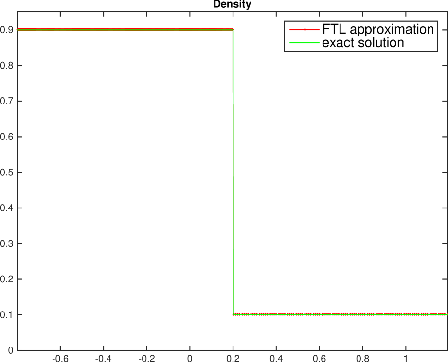
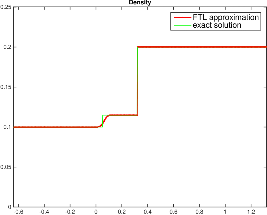
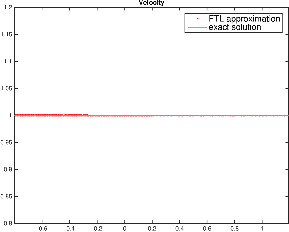
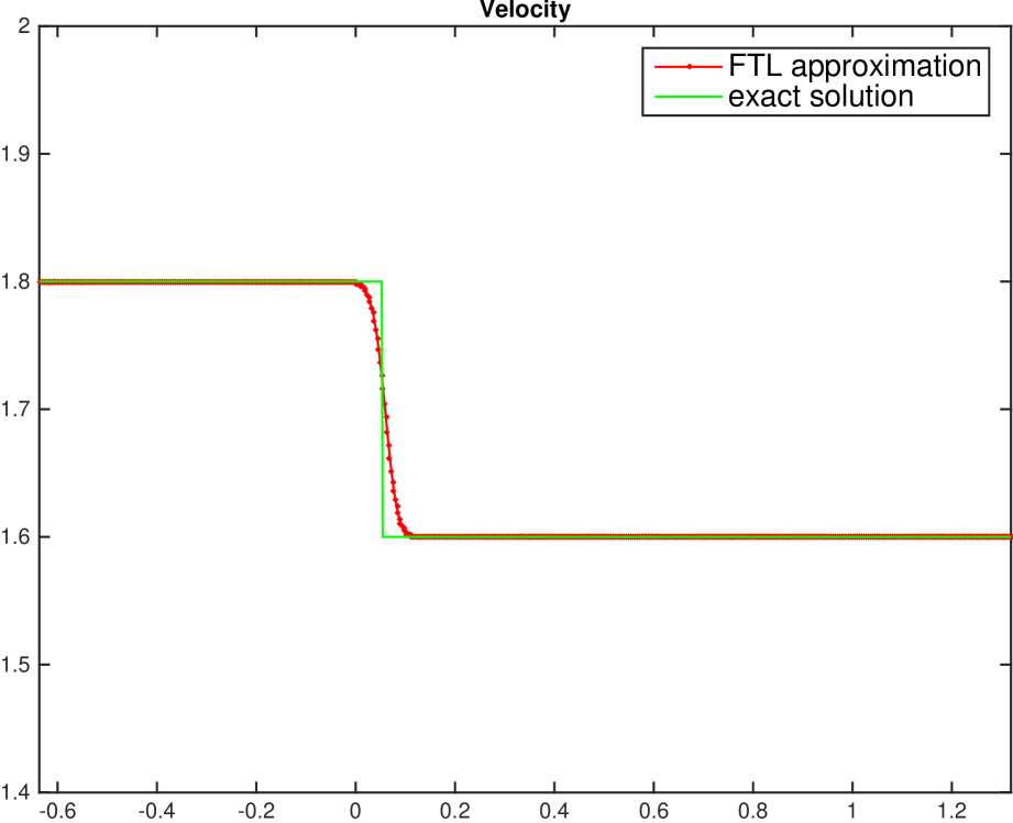
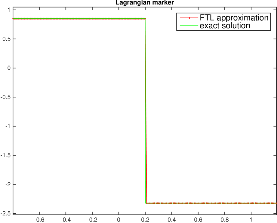
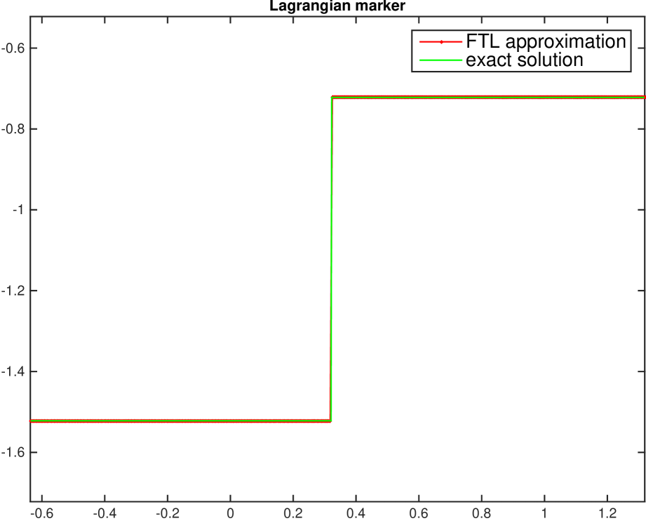
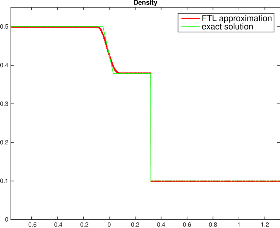
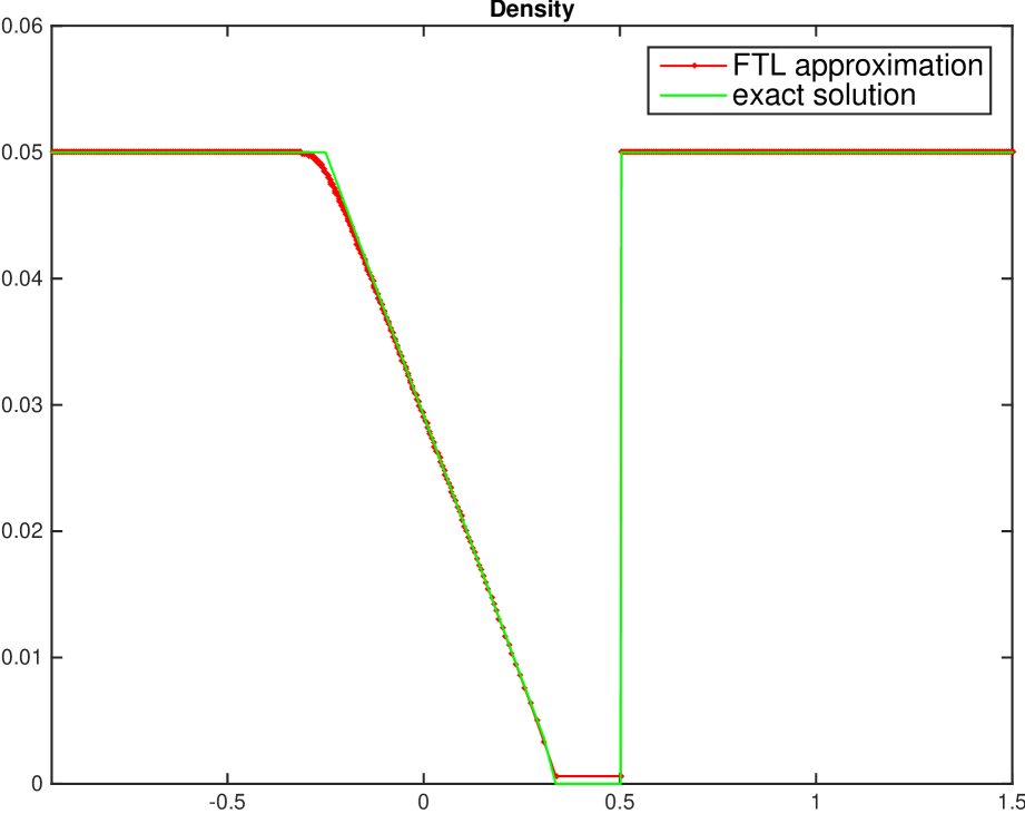
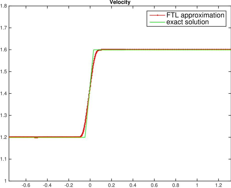
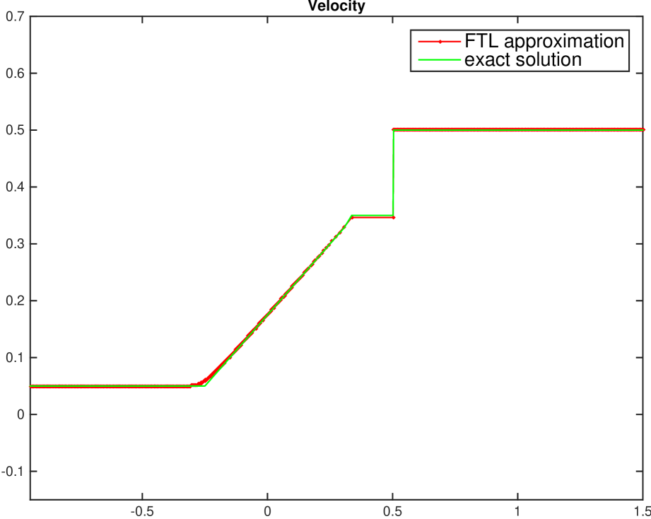
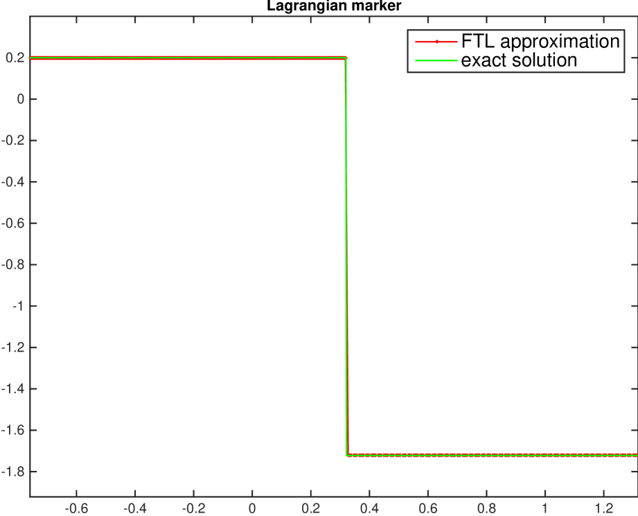
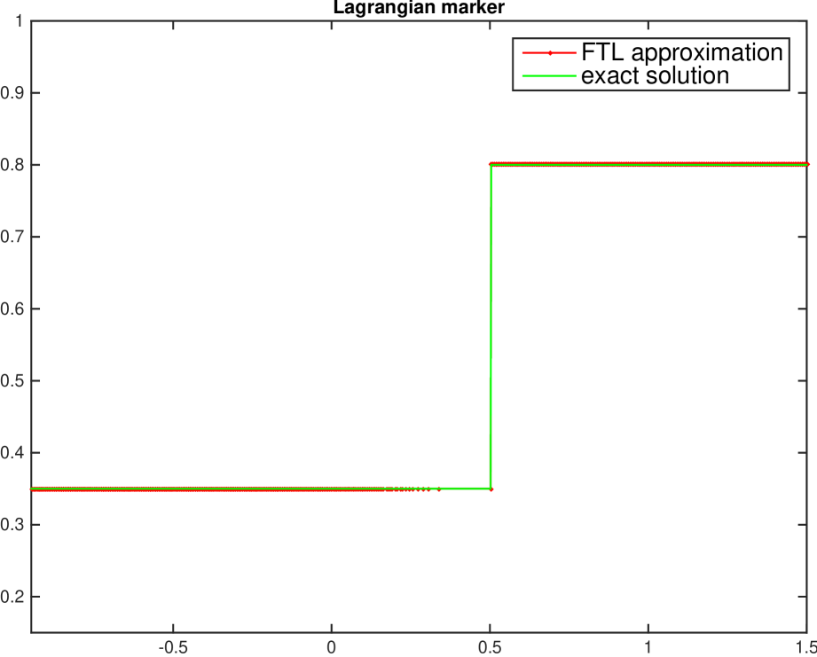
In order to test the proposed atomization algorithm, we consider four Riemann problems leading to four solutions of interest. The first three coincide with those done in [8, Section 4] and are used to check the ability of the scheme to deal with contact discontinuities. The last one is the example given in [3, Section 5] and is used to check the ability of the scheme to deal with the vacuum. In each case, the method is first evaluated by means of a qualitative comparison of the approximate solution ρΔsubscript𝜌Δ\rho_{\Delta}, vΔsubscript𝑣Δv_{\Delta}, wΔsubscript𝑤Δw_{\Delta} with the exact solution ρ𝜌\rho, v𝑣v, w𝑤w. Two initial mesh sizes are automatically determined by the total number of particles N𝑁N and the two density values of the Riemann data. The qualitative results corresponding to N=500𝑁500N=500 and final time t=0.2𝑡0.2t=0.2 for the Test 1, Test 2 and Test 3 and t=1𝑡1t=1 for Test 4 are presented on Figure 1 and Figure 2.

Test 1
p(ρ)=1.4427log(ρ)𝑝𝜌1.4427𝜌p(\rho)=1.4427\,\log(\rho),
ρ=0.9,v=1formulae-sequencesubscript𝜌0.9subscript𝑣1\rho_{\ell}=0.9,~{}v_{\ell}=1,
ρr=0.1,vr=1formulae-sequencesubscript𝜌𝑟0.1subscript𝑣𝑟1\rho_{r}=0.1,~{}v_{r}=1,
Test 2
p(ρ)=1.4427log(ρ)𝑝𝜌1.4427𝜌p(\rho)=1.4427\,\log(\rho),
ρ=0.1,v=1.8formulae-sequencesubscript𝜌0.1subscript𝑣1.8\rho_{\ell}=0.1,~{}v_{\ell}=1.8,
ρr=0.2,vr=1.6formulae-sequencesubscript𝜌𝑟0.2subscript𝑣𝑟1.6\rho_{r}=0.2,~{}v_{r}=1.6,
Refer to caption
Refer to caption
Refer to caption
Refer to caption
Refer to caption
Refer to caption
Figure 1. Left column for Test 1 and right column for Test 2. Initial conditions are specified in the tables on the top using N=200𝑁200N=200 particles.
Test 3
p(ρ)=1.4427log(ρ)𝑝𝜌1.4427𝜌p(\rho)=1.4427\,\log(\rho),
ρ=0.5,v=1.2formulae-sequencesubscript𝜌0.5subscript𝑣1.2\rho_{\ell}=0.5,~{}v_{\ell}=1.2,
ρr=0.1,vr=1.6formulae-sequencesubscript𝜌𝑟0.1subscript𝑣𝑟1.6\rho_{r}=0.1,~{}v_{r}=1.6,
Test 4
p(ρ)=6ρ𝑝𝜌6𝜌p(\rho)=6\rho,
ρ=0.05,v=0.05formulae-sequencesubscript𝜌0.05subscript𝑣0.05\rho_{\ell}=0.05,~{}v_{\ell}=0.05,
ρr=0.05,vr=0.5formulae-sequencesubscript𝜌𝑟0.05subscript𝑣𝑟0.5\rho_{r}=0.05,~{}v_{r}=0.5,
Refer to caption
Refer to caption
Refer to caption
Refer to caption
Refer to caption
Refer to caption
Figure 2. Left column for Test 3 and right column for Test 4. Initial conditions are specified in the tables on the top using N=200𝑁200N=200 particles.

Then, for several values of N𝑁N, a quantitative evaluation through the 𝐋𝟏superscript𝐋1\mathbf{L^{1}}-norm (of the difference between the exact and approximate densities solutions) is made, they are given on Table 1.

N𝑁N Test 1 Test 2 Test 3 Test 4
100 8.9e038.9𝑒038.9e-03 4.1e034.1𝑒034.1e-03 4.7e034.7𝑒034.7e-03 2.1e032.1𝑒032.1e-03
500 1.8e031.8𝑒031.8e-03 1.1e031.1𝑒031.1e-03 1.8e031.8𝑒031.8e-03 4.7e044.7𝑒044.7e-04
1000 4.7e044.7𝑒044.7e-04 5.7e045.7𝑒045.7e-04 1.2e031.2𝑒031.2e-03 2.5e042.5𝑒042.5e-04
2000 4.5e044.5𝑒044.5e-04 3.4e043.4𝑒043.4e-04 8.2e048.2𝑒048.2e-04 1.3e041.3𝑒041.3e-04
Table 1. Different numbers of particles and corresponding discrete 𝐋𝟏superscript𝐋1\mathbf{L^{1}}-errors for densities.

References

  • [1] B. Andreianov, C. Donadello, U. Razafison, J. Y. Rolland, and M. D. Rosini. Solutions of the Aw-Rascle-Zhang system with point constraints. Networks and Heterogeneous Media, 11(1):29–47, 2016.
  • [2] B. Andreianov, C. Donadello, and M. D. Rosini. A second-order model for vehicular traffics with local point constraints on the flow. Mathematical Models and Methods in Applied Sciences, 26(04):751–802, 2016.
  • [3] A. Aw, A. Klar, T. Materne, and M. Rascle. Derivation of continuum traffic flow models from microscopic Follow-the-Leader models. SIAM Journal on Applied Mathematics, 63(1):259–278, 2002.
  • [4] A. Aw and M. Rascle. Resurrection of “second order” models of traffic flow. SIAM Journal on Applied Mathematics, 60(3):916–938, 2000.
  • [5] P. Bagnerini and M. Rascle. A multi-class homogenized hyperbolic model of traffic flow. SIAM Journal of Mathematical Analysis, 35:2003, 2003.
  • [6] F. Berthelin, P. Degond, M. Delitala, and M. Rascle. A model for the formation and evolution of traffic jams. Archive for Rational Mechanics and Analysis, 187(2):185–220, 2008.
  • [7] A. Bressan. Hyperbolic systems of conservation laws: the one-dimensional Cauchy problem, volume 20. Oxford university press, 2000.
  • [8] C. Chalons and P. Goatin. Transport-equilibrium schemes for computing contact discontinuities in traffic flow modeling. Commun. Math. Sci., 5(3):533–551, 09 2007.
  • [9] M. Di Francesco, S. Fagioli, and M. D. Rosini. Deterministic particle approximation of scalar conservation laws. arXiv preprint arXiv:1605.05883, 2016.
  • [10] M. Di Francesco, S. Fagioli, M. D. Rosini, and G. Russo. Deterministic particle approximation of the Hughes model in one space dimension. arXiv preprint arXiv:1602.06153, 2016.
  • [11] M. Di Francesco, S. Fagioli, M. D. Rosini, and G. Russo. Follow-the-leader approximations of macroscopic models for vehicular and pedestrian flows. arXiv preprint, 2016.
  • [12] M. Di Francesco and M. Rosini. Rigorous derivation of nonlinear scalar conservation laws from Follow-the-Leader type models via many particle limit. Archive for Rational Mechanics and Analysis, 217(3):831–871, 2015.
  • [13] R. E. Ferreira and C. I. Kondo. Glimm method and wave-front tracking for the Aw-Rascle traffic flow model. Far East J. Math. Sci., 43:203–233, 2010.
  • [14] D. C. Gazis, R. Herman, and R. W. Rothery. Nonlinear Follow-the-Leader models of traffic flow. Operations Res., 9:545–567, 1961.
  • [15] M. Godvik and H. Hanche-Olsen. Existence of solutions for the Aw-Rascle traffic flow model with vacuum. Journal of Hyperbolic Differential Equations, 05(01):45–63, 2008.
  • [16] M. Lighthill and G. Whitham. On kinematic waves. II. A theory of traffic flow on long crowded roads. In Royal Society of London. Series A, Mathematical and Physical Sciences, volume 229, pages 317–345, 1955.
  • [17] S. Moutari and M. Rascle. A hybrid lagrangian model based on the Aw–Rascle traffic flow model. SIAM Journal on Applied Mathematics, 68(2):413–436, 2007.
  • [18] I. Prigogine and R. Herman. Kinetic theory of vehicular traffic. Elsevier, New York, 1971.
  • [19] P. I. Richards. Shock waves on the highway. Operations Research, 4(1):pp. 42–51, 1956.
  • [20] A. I. Vol’pert. The spaces BV and quasilinear equations. Mathematics of the USSR-Sbornik, 2(2):225, 1967.
  • [21] H. Zhang. A non-equilibrium traffic model devoid of gas-like behavior. Transportation Research Part B: Methodological, 36(3):275 – 290, 2002.

Received xxxx 20xx; revised xxxx 20xx.