An Efficient Multilinear Optimization Framework for Hypergraph Matching

Quynh Nguyen, Francesco Tudisco, Antoine Gautier, and Matthias Hein Q. Nguyen, F. Tudisco, A. Gautier and M. Hein are with the Department of Mathematics and Computer Science, Saarland University, Germany.
Corresponding Author: Quynh Nguyen.
E-mail: quynh@cs.uni-saarland.de
Abstract

Hypergraph matching has recently become a popular approach for solving correspondence problems in computer vision as it allows the use of higher-order geometric information. Hypergraph matching can be formulated as a third-order optimization problem subject to assignment constraints which turns out to be NP-hard. In recent work, we have proposed an algorithm for hypergraph matching which first lifts the third-order problem to a fourth-order problem and then solves the fourth-order problem via optimization of the corresponding multilinear form. This leads to a tensor block coordinate ascent scheme which has the guarantee of providing monotonic ascent in the original matching score function and leads to state-of-the-art performance both in terms of achieved matching score and accuracy. In this paper we show that the lifting step to a fourth-order problem can be avoided yielding a third-order scheme with the same guarantees and performance but being two times faster. Moreover, we introduce a homotopy type method which further improves the performance.

Index Terms:
Hypergraph Matching, Tensor, Multilinear Form, Block Coordinate Ascent

1 Introduction

Graph matching is among the most challenging tasks of graph processing and lies at the heart of various fields in pattern recognition, machine learning and computer vision. In computer vision, it has been used for solving several types of problems, for instance, object recognition [32], feature correspondence [11, 42], texture regularity discovery [20], shape matching [16, 38, 46], object tracking [2] and surface registration [48]. Graph matching also finds its applications in document processing tasks like optical character recognition [26, 17], image analysis (2D and 3D) [43, 33, 6, 37], or bioinformatics [39, 44, 41].

In this paper, we focus on the application of graph matching to the feature correspondence problem. Given sets of points/features extracted from two images, the task is to find for each point/feature in the first image a corresponding point/feature in the second image while maximizing as much as possible the similarity between them. The most simple first-order approach is to match each feature in the first set to its nearest neighbor in the second set by comparing their local descriptors. This naive approach fails in the presence of repeated patterns, textures or non-discriminative local appearances. To overcome this problem, second-order methods [27, 28, 29, 24, 9, 14, 42, 49, 50] try to enforce geometric consistency between pairs of correspondences, for instance using distances between points. However, pairwise relations are often not enough to capture the entire geometrical structure of point set. Therefore, higher-order approaches [47, 8, 15, 25, 48] that take into account higher-order relations between features/points have been proposed. This paper falls into this line of research. In particular, we cast the correspondence problem as a hypergraph matching problem using higher-order similarities instead of unary or pairwise ones used by previous methods. Depending on the chosen similarities, this formulation allows for both scaling and rotation invariance. However, instead of concentrating on how to build these similarities, see [15, 7, 19, 35], the focus of this paper is how to solve the resulting optimization problem.

Compared to graph matching, algorithms for hypergraph matching are less studied in the computer vision literature. The reason might be the difficult optimization problem which requires not only to deal with the combinatorial constraints but also to maximize a high degree polynomial function. Most prior work has relaxed the constraints in order to use concepts from continuous optimization [15, 25, 47, 8]. Our main idea is to reformulate the problem. Instead of maximizing a third-degree polynomial we maximize the corresponding multilinear form. This allows the direct integration of assignment constraints and yields a simple yet efficient block-coordinate ascent framework. The idea of this paper is based on our previous work [36], where the third-order problem has been lifted to a fourth-order problem in order to show the equivalence of maximizing the score function and its associated multilinear form. In this paper we show by a careful analysis that the lifting to a fourth-order problem can be avoided. The resulting third-order algorithms based on maximization of the third-order multilinear form have the same guarantees and properties as in [36] and achieve similar state-of-the-art matching score and matching accuracy while being two times faster. Moreover, we provide in this paper a quite generic framework, which allows the adaptation of our whole approach to matching problems with different assignment constraints, as well as to other general third-order optimization problems with combinatorial constraints.

Extensive experiments on both synthetic and realistic datasets show that all our algorithms, including the third-order and fourth-order ones, significantly outperform the current state-of-the-art in terms of both matching score and matching accuracy, in particular for very challenging settings where different kinds of noise are present in the data. In terms of running time, our algorithms are also on average significantly faster than previous approaches. All proofs and additional experimental results can be found in the appendix.

1.1 Related Work

The graph resp. hypergraph matching problem is known to be NP-hard except for special cases where polynomial-time algorithms exist e.g. for planar graphs [21]. In order to make the problem computationally tractable, a myriad of approximate algorithms have been proposed over the last three decades aiming at an acceptable trade-off between the complexity of the algorithm and matching accuracy. They can be categorized from different perspectives and we refer to [13, 18] for an extensive review. In this section, we review only those approximate algorithms that use Lawler’s formulations for both graph and hypergraph matching as they are closely related to our work. In particular, the graph matching problem can be formulated as a quadratic assignment problem (QAP)

max𝐱M𝐱TA𝐱subscriptmax𝐱𝑀superscript𝐱𝑇𝐴𝐱\mathop{\rm max}\nolimits\limits_{\mathbf{x}\in M}\mathbf{x}^{T}A\mathbf{x}

while the hypergraph matching problem is formulated as a higher-order assignment problem (HAP)

max𝐱Mi,j,k=1nijk𝐱i𝐱j𝐱ksubscriptmax𝐱𝑀superscriptsubscript𝑖𝑗𝑘1𝑛subscript𝑖𝑗𝑘subscript𝐱𝑖subscript𝐱𝑗subscript𝐱𝑘\mathop{\rm max}\nolimits\limits_{\mathbf{x}\in M}\sum_{i,j,k=1}^{n}\mathcal{F}_{ijk}\mathbf{x}_{i}\mathbf{x}_{j}\mathbf{x}_{k}

In these formulations, A𝐴A and \mathcal{F} refer to the affinity matrix and affinity tensor respectively, and M𝑀M is some matching constraint set depending on specific applications. Also, depending on whether the problem is graph matching or hypergraph matching, the corresponding algorithms will be called second-order methods or higher-order methods.

Among recent second-order methods, Leordeanu and Hebert [27] introduce the Spectral Matching (SM) algorithm, and Cour et al. [14] introduce Spectral Matching with Affine Constraint (SMAC). Both algorithms are based on the best rank-1 approximation of the affinity matrix. Torresani et al. [42] design a complex objective function which can be efficiently optimized by dual decomposition. Leordeanu et al. [29] propose the Integer Projected Fixed Point (IPFP) algorithm, which optimizes the quadratic objective function via a gradient-type algorithm interleaved with projection onto the assignment constraints using the Hungarian method. Lee et al. [24] tackle the graph matching problem using stochastic sampling, whereas Cho et al. [10] introduce a reweighted random walk (RRWM) where the reweighting is done in order to enforce the matching constraints. Zaslavskiy et al. [46] propose a path-following algorithm based on convex-concave relaxations. Zhou and Torre [49] factorize the affinity matrix and then compute a convex-concave relaxation of the objective function which is finally solved by a path-following method. Along this line there is also work of Liu et al. [31] and Zhou and Torre [50] extending previous methods [49, 46] to deal with directed graph matching. Recently, Cho et al. [12] propose a novel max pooling matching algorithm, in which they tweak the power method to better cope with noise in the affinities. Although the algorithm comes without theoretical guarantees, it turns out to perform very well in practice, in particular, when one has a large number of outliers.

The hypergraph matching problem (i.e. HAP) is much less studied in the literature. Duchenne et al. [15] formulate the hypergraph matching problem as a tensor eigenvalue problem and propose a higher-order power method for solving it. Zass and Shashua [47] introduce a probabilistic view on the problem with their Hypergraph Matching Method (HGM). Their idea is to marginalize the tensor to a vector and solve then the lower dimensional problem. Chertok and Keller [8] extend this idea and marginalize the tensor to a matrix, leading to a quadratic assignment problem which is then tackled using spectral methods. Since both methods are based on tensor marginalization, some part of the higher-order information is lost. Moreover, they cannot handle the one-to-one matching constraint during the iterations since it is only considered at the final discretization step. Lee et al. [25] extend the reweighted random walk approach of [24] to hypergraph matching. Their algorithm aims at enforcing the matching constraint via a bi-stochastic normalization scheme done at each iteration. In [48], Zeng et al. propose to use pseudo-boolean optimization [4] for 3D surface matching, where higher-order terms are decomposed into second-order terms and the quadratic pseudo-boolean optimization (QPBO) algorithm [22] is employed to solve the problem. We have proposed in [36] a tensor block-coordinate ascent framework, see also [45], for hypergraph matching based on a multilinear reformulation of the HAP where the third-order problem has been lifted to a fourth-order problem and one directly optimizes over the set of assignment matrices.

1.2 Notation

Vectors are denoted by bold lowercase letters (e.g. 𝐱𝐱\mathbf{x}). The elements of vectors are denoted by subscripts while superscripts denote iteration numbers. Tensors will be denoted by calligraphic uppercase letters (e.g. \mathcal{F}), while their associated multilinear forms will be denoted by the corresponding standard uppercase letter (e.g. F). The symbol tensor-product\otimes is used to denote the tensor product.

2 Hypergraph Matching Formulation

Hypergraphs are powerful in matching problems because they allow modeling of relations involving groups of more than two vertices so that higher-order information can be integrated. We concentrate our study on 333-uniform hypergraphs, i.e. each hyperedge describes a relation between up to 333 vertices. Every 333-uniform hypergraph can be represented by a third-order tensor. Let V𝑉V and Vsuperscript𝑉V^{\prime} be two point sets with n1=|V|n2=|V|subscript𝑛1𝑉subscript𝑛2superscript𝑉n_{1}=|V|\leq n_{2}=|V^{\prime}|. The matching problem consists of finding a binary assignment matrix X{0,1}n1×n2𝑋superscript01subscript𝑛1subscript𝑛2X\in\{0,1\}^{n_{1}\times n_{2}} such that Xij=1subscript𝑋𝑖𝑗1X_{ij}=1 if viVsubscript𝑣𝑖𝑉v_{i}\in V matches vjV,subscriptsuperscript𝑣𝑗superscript𝑉v^{\prime}_{j}\in V^{\prime}, and Xij=0subscript𝑋𝑖𝑗0X_{ij}=0 otherwise. The set of all possible assignment matrices that assign each vertex of V𝑉V to exactly one vertex of Vsuperscript𝑉V^{\prime} is given by

M={X{0,1}n1×n2|i=1n1Xij1,j=1n2Xij=1}.𝑀conditional-set𝑋superscript01subscript𝑛1subscript𝑛2formulae-sequencesuperscriptsubscript𝑖1subscript𝑛1subscript𝑋𝑖𝑗1superscriptsubscript𝑗1subscript𝑛2subscript𝑋𝑖𝑗1M=\big{\{}X\in\{0,1\}^{n_{1}\times n_{2}}\,\big{|}\,\sum_{i=1}^{n_{1}}X_{ij}\leq 1,\quad\sum_{j=1}^{n_{2}}X_{ij}=1\big{\}}.

Suppose that we have a function :(V×V)3+:superscript𝑉superscript𝑉3subscript\mathcal{F}:(V\times V^{\prime})^{3}\to\mathbb{R}_{+} which maps each pair of triples {vi1,vi2,vi3}Vsubscript𝑣subscript𝑖1subscript𝑣subscript𝑖2subscript𝑣subscript𝑖3𝑉\{v_{i_{1}},v_{i_{2}},v_{i_{3}}\}\subset V and {vj1,vj2,vj3}Vsubscriptsuperscript𝑣subscript𝑗1subscriptsuperscript𝑣subscript𝑗2subscriptsuperscript𝑣subscript𝑗3superscript𝑉\{v^{\prime}_{j_{1}},v^{\prime}_{j_{2}},v^{\prime}_{j_{3}}\}\subset V^{\prime} to its similarity weight (i1,j1),(i2,j2),(i3,j3)subscriptsubscript𝑖1subscript𝑗1subscript𝑖2subscript𝑗2subscript𝑖3subscript𝑗3\mathcal{F}_{(i_{1},j_{1}),(i_{2},j_{2}),(i_{3},j_{3})}. For example, \mathcal{F} is calculated as the similarity of the corresponding angles of the two triangles i1j1k1subscript𝑖1subscript𝑗1subscript𝑘1\bigtriangleup i_{1}j_{1}k_{1} and i2j2k2subscript𝑖2subscript𝑗2subscript𝑘2\bigtriangleup i_{2}j_{2}k_{2} as shown in Fig. 1. Then, the score S(X)𝑆𝑋S(X) of a matching XM𝑋𝑀X\in M is defined as follows [15]

S(X)=i1,i2,i3=1n1j1,j2,j3=1n2(i1,j1),(i2,j2),(i3,j3)Xi1j1Xi2j2Xi3j3.𝑆𝑋superscriptsubscriptsubscript𝑖1subscript𝑖2subscript𝑖31subscript𝑛1superscriptsubscriptsubscript𝑗1subscript𝑗2subscript𝑗31subscript𝑛2subscriptsubscript𝑖1subscript𝑗1subscript𝑖2subscript𝑗2subscript𝑖3subscript𝑗3subscript𝑋subscript𝑖1subscript𝑗1subscript𝑋subscript𝑖2subscript𝑗2subscript𝑋subscript𝑖3subscript𝑗3S(X)=\!\!\!\!\!\sum_{i_{1},i_{2},i_{3}=1}^{n_{1}}\sum_{j_{1},j_{2},j_{3}=1}^{n_{2}}\!\!\!\!\mathcal{F}_{(i_{1},j_{1}),(i_{2},j_{2}),(i_{3},j_{3})}X_{i_{1}j_{1}}X_{i_{2}j_{2}}X_{i_{3}j_{3}}.

For ease of notation, we introduce a linear ordering in V×V𝑉superscript𝑉V\times V^{\prime} so that each XM𝑋𝑀X\in M can be rewritten as a vector 𝐱{0,1}n𝐱superscript01𝑛\mathbf{x}\in\{0,1\}^{n} with n=n1n2𝑛subscript𝑛1subscript𝑛2n=n_{1}n_{2} and \mathcal{F} as a tensor in n×n×nsuperscript𝑛𝑛𝑛\mathbb{R}^{n\times n\times n}. With this convention, the score function S:n:𝑆superscript𝑛S:\mathbb{R}^{n}\to\mathbb{R} can be computed in the following way

S(𝐱)=i,j,k=1nijk𝐱i𝐱j𝐱k.𝑆𝐱superscriptsubscript𝑖𝑗𝑘1𝑛subscript𝑖𝑗𝑘subscript𝐱𝑖subscript𝐱𝑗subscript𝐱𝑘S(\mathbf{x})=\sum_{i,j,k=1}^{n}\mathcal{F}_{ijk}\,\mathbf{x}_{i}\,\mathbf{x}_{j}\,\mathbf{x}_{k}. (1)

We recall that a third-order tensor 𝒯n×n×n𝒯superscript𝑛𝑛𝑛\mathcal{T}\in\mathbb{R}^{n\times n\times n} is called symmetric if its entries 𝒯ijksubscript𝒯𝑖𝑗𝑘\mathcal{T}_{ijk} are invariant under any permutation of {i,j,k}𝑖𝑗𝑘\{i,j,k\}. In particular, the tensor 𝒯ijk:=𝐱i𝐱j𝐱kassignsubscript𝒯𝑖𝑗𝑘subscript𝐱𝑖subscript𝐱𝑗subscript𝐱𝑘\mathcal{T}_{ijk}:=\mathbf{x}_{i}\mathbf{x}_{j}\mathbf{x}_{k} is symmetric and thus the non-symmetric part of \mathcal{F} is “averaged” out in the computation of S(𝐱)𝑆𝐱S(\mathbf{x}). Therefore, without loss of generality, we can assume that \mathcal{F} is symmetric111Note that \mathcal{F} can always be symmetrized (without changing the score function) as follows ~ijk=13!σ𝔖3σ(i)σ(j)σ(k)subscript~𝑖𝑗𝑘13subscript𝜎subscript𝔖3subscript𝜎𝑖𝜎𝑗𝜎𝑘\tilde{\mathcal{F}}_{ijk}=\frac{1}{3!}\sum_{\sigma\in\mathfrak{S}_{3}}\mathcal{F}_{\sigma(i)\sigma(j)\sigma(k)}, where i,j,k=1,,nformulae-sequence𝑖𝑗𝑘1𝑛i,j,k=1,\ldots,n and 𝔖3subscript𝔖3\mathfrak{S}_{3} is the permutation group of three elements.. In this paper, we consider only terms of order 333, i.e. ijk=0subscript𝑖𝑗𝑘0\mathcal{F}_{ijk}=0 if i=j𝑖𝑗i=j, i=k𝑖𝑘i=k or j=k𝑗𝑘j=k. However, note that it is possible to integrate first-order terms on the main diagonal iiisubscript𝑖𝑖𝑖\mathcal{F}_{iii}, and pairwise potentials ijjsubscript𝑖𝑗𝑗\mathcal{F}_{ijj} for ij𝑖𝑗i\neq j. This is also the major advantage of hypergraph matching over conventional graph matching methods because one can combine local appearance similarities, pair-wise similarities (e.g. distances) and higher-order invariants (e.g. angles of triplets of points) in a unified framework.

i1subscript𝑖1i_{1}j1subscript𝑗1j_{1}k1subscript𝑘1k_{1}i2subscript𝑖2i_{2}j2subscript𝑗2j_{2}k2subscript𝑘2k_{2}
Figure 1: Illustration of constructing the affinity tensor. Each entry is computed by comparing the angles of two triangles formed by three candidate correspondences (i1,i2),(j1,j2)subscript𝑖1subscript𝑖2subscript𝑗1subscript𝑗2(i_{1},i_{2}),(j_{1},j_{2}) and (k1,k2)subscript𝑘1subscript𝑘2(k_{1},k_{2}).

3 Mathematical Foundations for Multilinear Optimization Framework

In this section, we derive the basis for our tensor block coordinate ascent framework for solving hypergraph matching problems. The general idea is to optimize instead of the score function S𝑆S the associated third-order multilinear form F:n×n×n:Fsuperscript𝑛superscript𝑛superscript𝑛\textit{F}\colon\mathbb{R}^{n}\times\mathbb{R}^{n}\times\mathbb{R}^{n}\to\mathbb{R} which is defined as

F(𝐱,𝐲,𝐳)=i,j,k=1nijk𝐱i𝐲j𝐳k.F𝐱𝐲𝐳superscriptsubscript𝑖𝑗𝑘1𝑛subscript𝑖𝑗𝑘subscript𝐱𝑖subscript𝐲𝑗subscript𝐳𝑘\textit{F}(\mathbf{x},\mathbf{y},\mathbf{z})=\sum_{i,j,k=1}^{n}\mathcal{F}_{ijk}\,\mathbf{x}_{i}\,\mathbf{y}_{j}\,\mathbf{z}_{k}. (2)

It turns out that the score function in Eq. (1) is a special case of the multilinear form when all the arguments are the same, i.e. S(𝐱)=F(𝐱,𝐱,𝐱).𝑆𝐱F𝐱𝐱𝐱S(\mathbf{x})=\textit{F}(\mathbf{x},\mathbf{x},\mathbf{x}). The multilinear form is called symmetric if it is invariant under any permutation of its arguments, i.e. F(𝐱1,𝐱2,𝐱3)=F(𝐱σ(1),𝐱σ(2),𝐱σ(3))Fsuperscript𝐱1superscript𝐱2superscript𝐱3Fsuperscript𝐱𝜎1superscript𝐱𝜎2superscript𝐱𝜎3\textit{F}(\mathbf{x}^{1},\mathbf{x}^{2},\mathbf{x}^{3})=\textit{F}(\mathbf{x}^{\sigma(1)},\mathbf{x}^{\sigma(2)},\mathbf{x}^{\sigma(3)}) for all 𝐱1,𝐱2,𝐱3nsuperscript𝐱1superscript𝐱2superscript𝐱3superscript𝑛\mathbf{x}^{1},\mathbf{x}^{2},\mathbf{x}^{3}\in\mathbb{R}^{n} and σ𝜎\sigma a permutation of {1,2,3}.123\{1,2,3\}. Note that if the tensor \mathcal{F} is symmetric then F is also symmetric. In the following, we write F(,𝐲,𝐳)F𝐲𝐳\textit{F}(\,\cdot\,,\mathbf{y},\mathbf{z}) to denote a vector in nsuperscript𝑛\mathbb{R}^{n} such that F(,𝐲,𝐳)i=j,k=1nijk𝐲j𝐳kFsubscript𝐲𝐳𝑖superscriptsubscript𝑗𝑘1𝑛subscript𝑖𝑗𝑘subscript𝐲𝑗subscript𝐳𝑘\textit{F}(\,\cdot\,,\mathbf{y},\mathbf{z})_{i}=\sum_{j,k=1}^{n}\mathcal{F}_{ijk}\mathbf{y}_{j}\mathbf{z}_{k} for all 1in,1𝑖𝑛1\leq i\leq n, and write F(,,𝐳)F𝐳\textit{F}(\,\cdot\,,\,\cdot\,,\mathbf{z}) to denote a matrix in n×nsuperscript𝑛𝑛\mathbb{R}^{n\times n} such that F(,,𝐳)ij=k=1nijk𝐳kFsubscript𝐳𝑖𝑗superscriptsubscript𝑘1𝑛subscript𝑖𝑗𝑘subscript𝐳𝑘\textit{F}(\,\cdot\,,\,\cdot\,,\mathbf{z})_{ij}=\sum_{k=1}^{n}\mathcal{F}_{ijk}\mathbf{z}_{k} for all 1i,jn.formulae-sequence1𝑖𝑗𝑛1\leq i,j\leq n. Note that the positions of the dots do not matter in the case of a symmetric multilinear form because the function is invariant under any permutation of its arguments.

The hypergraph matching problem can be written as the maximization of a third-order score function S𝑆S subject to the assignment constraints,

max𝐱MS(𝐱)=max𝐱MF(𝐱,𝐱,𝐱)=max𝐱Mi,j,k=1nijk𝐱i𝐱j𝐱k.subscriptmax𝐱𝑀𝑆𝐱subscriptmax𝐱𝑀F𝐱𝐱𝐱subscriptmax𝐱𝑀superscriptsubscript𝑖𝑗𝑘1𝑛subscript𝑖𝑗𝑘subscript𝐱𝑖subscript𝐱𝑗subscript𝐱𝑘\displaystyle\mathop{\rm max}\nolimits\limits_{\mathbf{x}\in M}S(\mathbf{x})=\mathop{\rm max}\nolimits\limits_{\mathbf{x}\in M}\textit{F}(\mathbf{x},\mathbf{x},\mathbf{x})=\mathop{\rm max}\nolimits\limits_{\mathbf{x}\in M}\sum_{i,j,k=1}^{n}\mathcal{F}_{ijk}\,\mathbf{x}_{i}\,\mathbf{x}_{j}\,\mathbf{x}_{k}. (3)

In [36] we propose to solve instead the equivalent problem defined as

max𝐱MS4(𝐱)=max𝐱MF4(𝐱,𝐱,𝐱,𝐱):=i,j,k,l=1nijkl4𝐱i𝐱j𝐱k𝐱lsubscriptmax𝐱𝑀superscript𝑆4𝐱subscriptmax𝐱𝑀superscriptF4𝐱𝐱𝐱𝐱assignsuperscriptsubscript𝑖𝑗𝑘𝑙1𝑛subscriptsuperscript4𝑖𝑗𝑘𝑙subscript𝐱𝑖subscript𝐱𝑗subscript𝐱𝑘subscript𝐱𝑙\displaystyle\mathop{\rm max}\nolimits\limits_{\mathbf{x}\in M}S^{4}(\mathbf{x})=\mathop{\rm max}\nolimits\limits_{\mathbf{x}\in M}\textit{F}^{4}(\mathbf{x},\mathbf{x},\mathbf{x},\mathbf{x}){\color[rgb]{0,0,0}\definecolor[named]{pgfstrokecolor}{rgb}{0,0,0}\pgfsys@color@gray@stroke{0}\pgfsys@color@gray@fill{0}:=}\sum_{i,j,k,l=1}^{n}\mathcal{F}^{4}_{ijkl}\mathbf{x}_{i}\mathbf{x}_{j}\mathbf{x}_{k}\mathbf{x}_{l} (4)

where the new symmetric fourth-order tensor 4superscript4\mathcal{F}^{4} is obtained by lifting the third order tensor \mathcal{F} via

ijkl4=ijk+ijl+ikl+jkl.subscriptsuperscript4𝑖𝑗𝑘𝑙subscript𝑖𝑗𝑘subscript𝑖𝑗𝑙subscript𝑖𝑘𝑙subscript𝑗𝑘𝑙\mathcal{F}^{4}_{ijkl}=\mathcal{F}_{ijk}+\mathcal{F}_{ijl}+\mathcal{F}_{ikl}+\mathcal{F}_{jkl}. (5)

The reason for this lifting step is discussed below. The main idea of [36] is then to optimize instead of the score function the associated multilinear form. The following theorem establishes equivalence of these problems under the assumption that the score function S4superscript𝑆4S^{4} is convex on nsuperscript𝑛\mathbb{R}^{n}.

Theorem 3.1 (Nguyen et al. [36])

Let 4superscript4\mathcal{F}^{4} be a symmetric fourth-order tensor and suppose the corresponding score function S4:n:superscript𝑆4superscript𝑛S^{4}\colon\mathbb{R}^{n}\to\mathbb{R} is convex. Then it holds for any compact constraint set Dn𝐷superscript𝑛D\subset\mathbb{R}^{n},

max𝐱DF4(𝐱,𝐱,𝐱,𝐱)subscriptmax𝐱𝐷superscriptF4𝐱𝐱𝐱𝐱\displaystyle\mathop{\rm max}\nolimits\limits_{\mathbf{x}\in D}\textit{F}^{4}(\mathbf{x},\mathbf{x},\mathbf{x},\mathbf{x})\!\!\! =\displaystyle= max𝐱,𝐲DF4(𝐱,𝐱,𝐲,𝐲)subscriptmax𝐱𝐲𝐷superscriptF4𝐱𝐱𝐲𝐲\displaystyle\!\!\!\mathop{\rm max}\nolimits\limits_{\mathbf{x},\mathbf{y}\in D}\textit{F}^{4}(\mathbf{x},\mathbf{x},\mathbf{y},\mathbf{y})
=\displaystyle= max𝐱,𝐲,𝐳,𝐭DF4(𝐱,𝐲,𝐳,𝐭).subscriptmax𝐱𝐲𝐳𝐭𝐷superscriptF4𝐱𝐲𝐳𝐭\displaystyle\!\!\!\mathop{\rm max}\nolimits\limits_{\mathbf{x},\mathbf{y},\mathbf{z},\mathbf{t}\in D}\textit{F}^{4}(\mathbf{x},\mathbf{y},\mathbf{z},\mathbf{t}).

Note that a given score function S4superscript𝑆4S^{4} need not be convex. In [36] we show that every fourth-order score function can be modified so that it becomes convex, while solving (4) for the original and the modified score function turns out to be equivalent. The maximization of the multilinear form F4(𝐱,𝐲,𝐳,𝐭)superscriptF4𝐱𝐲𝐳𝐭\textit{F}^{4}(\mathbf{x},\mathbf{y},\mathbf{z},\mathbf{t}) can then be done in two ways. Either one fixes all but one or all but two arguments and maximizes the remaining arguments over the set of assignment matrices M𝑀M. As shown in [36], this scheme boils down to solving a sequence of Linear Assignment Problems (LAPs) or a sequence of (approximate) QAPs which can be done efficiently by existing lower-order methods.

The convexity of the score function is crucial for the proof of Theorem 3.1. The lifting step (5) has been proposed in [36] as non-trivial third-order score functions are not convex on nsuperscript𝑛\mathbb{R}^{n} as the following lemma shows.

Lemma 3.2 (Nguyen et al. [36])

Let S𝑆S be a third-order score function defined as in Eq. (1). If S𝑆S is not constant zero, then S:n:𝑆superscript𝑛S:\mathbb{R}^{n}\to\mathbb{R} is not convex.

In the following we show that a statement similar to Theorem 3.1 holds also in the third-order case. This allows us to propose algorithms directly for the third-order case without the lifting step, leading to two times faster algorithms. The new key insight to establish this result is that convexity on whole nsuperscript𝑛\mathbb{R}^{n} is not required. If one just requires that the third-order score function is convex on the positive orthant, then Lemma 3.2 is no longer true. In fact convexity is only required in a “pointwise” fashion which we make precise in Theorem 3.3. Similar to our previous Theorem 3.1, we state the main Theorem 3.3 of this paper for general compact sets Dn𝐷superscript𝑛D\subset\mathbb{R}^{n} which includes as a special case the set of assignment matrices. Although this general form of the theorem may allow generalizations of our proposed framework to other applications, in this paper we only focus on the case D=M𝐷𝑀D=M for the application of hypergraph matching.

Theorem 3.3

Let Dn𝐷superscript𝑛D\subset\mathbb{R}^{n} be a compact set, F:n×n×n:Fsuperscript𝑛superscript𝑛superscript𝑛\textit{F}:\mathbb{R}^{n}\times\mathbb{R}^{n}\times\mathbb{R}^{n}\to\mathbb{R} a symmetric third-order multilinear form and S:n:𝑆superscript𝑛S:\mathbb{R}^{n}\to\mathbb{R} the associated third-order score function such that S(𝐱)=F(𝐱,𝐱,𝐱),𝑆𝐱𝐹𝐱𝐱𝐱S(\mathbf{x})=F(\mathbf{x},\mathbf{x},\mathbf{x}), then we have the following chain of implications: 1) \Rightarrow 2) \Rightarrow 3) \Rightarrow 4).

  1. 1.

    2S(𝐱)superscript2𝑆𝐱\nabla^{2}S(\mathbf{x}) is positive semidefinite for all 𝐱D.𝐱𝐷\mathbf{x}\in D.

  2. 2.

    F(𝐱,𝐲𝐳,𝐲𝐳)0F𝐱𝐲𝐳𝐲𝐳0\textit{F}(\mathbf{x},\mathbf{y}-\mathbf{z},\mathbf{y}-\mathbf{z})\geq 0 for all 𝐱,𝐲,𝐳D.𝐱𝐲𝐳𝐷\mathbf{x},\mathbf{y},\mathbf{z}\in D.

  3. 3.

    It holds for all 𝐱,𝐲,𝐳D𝐱𝐲𝐳𝐷\mathbf{x},\mathbf{y},\mathbf{z}\in D

    F(𝐱,𝐲,𝐳)max𝐮{𝐱,𝐲,𝐳}F(𝐮,𝐮,𝐮).F𝐱𝐲𝐳subscriptmax𝐮𝐱𝐲𝐳F𝐮𝐮𝐮\textit{F}(\mathbf{x},\mathbf{y},\mathbf{z})\leq\mathop{\rm max}\nolimits\limits_{\mathbf{u}\in\{\mathbf{x},\mathbf{y},\mathbf{z}\}}\textit{F}(\mathbf{u},\mathbf{u},\mathbf{u}). (6)
  4. 4.

    The optimization of the multilinear form is equivalent to the optimization of its associated score function

    max𝐱,𝐲,𝐳DF(𝐱,𝐲,𝐳)=max𝐱,𝐲DF(𝐱,𝐱,𝐲)=max𝐱DF(𝐱,𝐱,𝐱).subscriptmax𝐱𝐲𝐳𝐷F𝐱𝐲𝐳subscriptmax𝐱𝐲𝐷F𝐱𝐱𝐲subscriptmax𝐱𝐷F𝐱𝐱𝐱\!\!\!\!\mathop{\rm max}\nolimits\limits_{\mathbf{x},\mathbf{y},\mathbf{z}\in D}\textit{F}(\mathbf{x},\mathbf{y},\mathbf{z})=\mathop{\rm max}\nolimits\limits_{\mathbf{x},\mathbf{y}\in D}\textit{F}(\mathbf{x},\mathbf{x},\mathbf{y})=\mathop{\rm max}\nolimits\limits_{\mathbf{x}\in D}\textit{F}(\mathbf{x},\mathbf{x},\mathbf{x}).

As a twice continuously differentiable function is convex if and only if its Hessian is positive semi-definite on its domain, the first requirement is much weaker than requiring convexity on whole nsuperscript𝑛\mathbb{R}^{n}. Thus Theorem 3.3 allows us to establish for D=M𝐷𝑀D=M inequality (6) for a nontrivial class of third-order score functions, which is the key result necessary to establish the equivalence of the maximization of the score function and the maximization of the multilinear form. This is the key requirement to show monotonic ascent for our block-coordinate optimization scheme. In Proposition 3.4 we show how to modify an existing third-order score function so that it satisfies condition 1) for D=M𝐷𝑀D=M. Again this modification turns out to be constant on M𝑀M and thus leads to equivalent optimization problems. This altogether leads to two new algorithms for the hypergraph matching problem (1) similar to our previous work [36]. The key idea of both algorithms is to use block-coordinate ascent updates, where all but one argument or all but two arguments of the multilinear form are fixed and one optimizes over the remaining ones in either case. The inequality (6) then allows us to connect the solutions of the two optimization problems. In both variants, we directly optimize over the discrete set M𝑀M of possible matchings, that is, there is no relaxation involved. Moreover, we theoretically prove monotonic ascent for both methods. In all our experiments, the proposed third-order methods achieve competitive matching score and matching accuracy to the fourth-order ones [36] while outperforming other state-of-the-art approaches. On the other hand, we achieve a speed up of factor 222 over the fourth-order algorithms due to the ability of working directly with the original tensor.

Compared to [36] we avoid the lifting step while maintaining the same theoretical guarantees. Moreover, we use the weaker conditions on the score function in Theorem 3.3 to propose two variants of our algorithms based on homotopy methods as presented in Section 3.3.

In general, the multilinear form F might not fulfill the conditions of Theorem 3.3. Therefore, we propose to modify F by adding to it some multilinear form G so that the first statement of Theorem 3.3 is satisfied for the new function. At the same time the modification does not affect the solution of our problem since the added term is constant on the set of assignment matrices. This will be detailed later on in Proposition 3.4. While finding the best possible modification is difficult, one can consider some canonical choices. As the first choice, one can implicitly modify F by considering a new score function defined as Sα(𝐱)=S(𝐱)+α𝐱22,subscript𝑆𝛼𝐱𝑆𝐱𝛼superscriptsubscriptnorm𝐱22{\color[rgb]{0,0,0}\definecolor[named]{pgfstrokecolor}{rgb}{0,0,0}\pgfsys@color@gray@stroke{0}\pgfsys@color@gray@fill{0}S_{\alpha}(\mathbf{x})}=S(\mathbf{x})+\alpha\left\|\mathbf{x}\right\|_{2}^{2}, and then show that there exists some α0subscript𝛼0\alpha_{0}\in\mathbb{R} such that 2Sαsuperscript2subscript𝑆𝛼\nabla^{2}S_{\alpha} is positive semidefinite everywhere in M𝑀M for all αα0.𝛼subscript𝛼0\alpha\geq\alpha_{0}. However, the modified score function Sαsubscript𝑆𝛼S_{\alpha} then becomes in-homogeneous and thus there does not exist any multilinear form Fαsubscript𝐹𝛼F_{\alpha} such that Sα(𝐱)=Fα(𝐱,𝐱,𝐱).subscript𝑆𝛼𝐱subscript𝐹𝛼𝐱𝐱𝐱{\color[rgb]{0,0,0}\definecolor[named]{pgfstrokecolor}{rgb}{0,0,0}\pgfsys@color@gray@stroke{0}\pgfsys@color@gray@fill{0}S_{\alpha}(\mathbf{x})=F_{\alpha}(\mathbf{x},\mathbf{x},\mathbf{x})}.

A homogeneous modification would be Sα(𝐱)=S(𝐱)+α𝐱33subscript𝑆𝛼𝐱𝑆𝐱𝛼superscriptsubscriptnorm𝐱33{\color[rgb]{0,0,0}\definecolor[named]{pgfstrokecolor}{rgb}{0,0,0}\pgfsys@color@gray@stroke{0}\pgfsys@color@gray@fill{0}S_{\alpha}(\mathbf{x})}=S(\mathbf{x})+\alpha\left\|\mathbf{x}\right\|_{3}^{3}. Indeed, one can associate to 𝐱33superscriptsubscriptnorm𝐱33\left\|\mathbf{x}\right\|_{3}^{3} the multilinear form G(𝐱,𝐲,𝐳)=i=1n𝐞i,𝐱𝐞i,𝐲𝐞i,𝐳,G𝐱𝐲𝐳superscriptsubscript𝑖1𝑛subscript𝐞𝑖𝐱subscript𝐞𝑖𝐲subscript𝐞𝑖𝐳\textit{G}(\mathbf{x},\mathbf{y},\mathbf{z})=\sum_{i=1}^{n}\left\langle{\mathbf{e}}_{i},\mathbf{x}\right\rangle\left\langle{\mathbf{e}}_{i},\mathbf{y}\right\rangle\left\langle{\mathbf{e}}_{i},\mathbf{z}\right\rangle, where 𝐞isubscript𝐞𝑖\mathbf{e}_{i} is the i𝑖i-th standard basis vector of n.superscript𝑛\mathbb{R}^{n}. Moreover, it holds that G(𝐱,𝐱,𝐱)=𝐱33.G𝐱𝐱𝐱superscriptsubscriptnorm𝐱33\textit{G}(\mathbf{x},\mathbf{x},\mathbf{x})=\left\|\mathbf{x}\right\|_{3}^{3}. In this paper, we consider a family of modifications which includes the one above by perturbing the set of basis vectors as 𝐞¯i=ε𝟏+(1ε)𝐞isubscript¯𝐞𝑖𝜀11𝜀subscript𝐞𝑖\bar{\mathbf{e}}_{i}=\varepsilon\mathbf{1}+(1-\varepsilon)\mathbf{e}_{i} with 𝟏1\mathbf{1} being the all-ones vector. Note that 𝐱33superscriptsubscriptnorm𝐱33\left\|\mathbf{x}\right\|_{3}^{3} is included in this family as a special case for ε=0.𝜀0\varepsilon=0. The main idea is that one can later on optimize ε𝜀\varepsilon to find the best lower bound on α.𝛼\alpha. That is to say, we aim at a minimal amount of S𝑆S such that the conditions from Theorem 3.3 are satisfied. As shown in the proof of Proposition 3.4, ε=1/3𝜀13\varepsilon=1/3 is the optimal value for which the best bound on α𝛼\alpha can be obtained. Thus, we use this value in the rest of the paper. In particular, let 𝐞¯i=13𝟏+23𝐞isubscript¯𝐞𝑖13123subscript𝐞𝑖\bar{\mathbf{e}}_{i}=\frac{1}{3}\mathbf{1}+\frac{2}{3}\mathbf{e}_{i} we define the symmetric third-order tensor 𝒢𝒢\mathcal{G} as

𝒢=i=1n𝐞¯i𝐞¯i𝐞¯i,𝒢superscriptsubscript𝑖1𝑛tensor-productsubscript¯𝐞𝑖subscript¯𝐞𝑖subscript¯𝐞𝑖\mathcal{G}=\sum_{i=1}^{n}\bar{\mathbf{e}}_{i}\otimes\bar{\mathbf{e}}_{i}\otimes\bar{\mathbf{e}}_{i}, (7)

and the associated multilinear form as

G(𝐱,𝐲,𝐳)=i=1n𝐞¯i,𝐱𝐞¯i,𝐲𝐞¯i,𝐳.G𝐱𝐲𝐳superscriptsubscript𝑖1𝑛subscript¯𝐞𝑖𝐱subscript¯𝐞𝑖𝐲subscript¯𝐞𝑖𝐳\textit{G}(\mathbf{x},\mathbf{y},\mathbf{z})=\sum_{i=1}^{n}\left\langle\bar{\mathbf{e}}_{i},\mathbf{x}\right\rangle\left\langle\bar{\mathbf{e}}_{i},\mathbf{y}\right\rangle\left\langle\bar{\mathbf{e}}_{i},\mathbf{z}\right\rangle. (8)
Proposition 3.4

Let F:n×n×n:Fsuperscript𝑛superscript𝑛superscript𝑛\textit{F}:\mathbb{R}^{n}\times\mathbb{R}^{n}\times\mathbb{R}^{n}\to\mathbb{R} be a symmetric third-order multilinear form and G:n×n×n:Gsuperscript𝑛superscript𝑛superscript𝑛\textit{G}:\mathbb{R}^{n}\times\mathbb{R}^{n}\times\mathbb{R}^{n}\to\mathbb{R} as defined in Eq. (8). We consider the new multilinear form FαsubscriptF𝛼\textit{F}_{\alpha} defined by

Fα(𝐱,𝐲,𝐳)=F(𝐱,𝐲,𝐳)+αG(𝐱,𝐲,𝐳).subscriptF𝛼𝐱𝐲𝐳F𝐱𝐲𝐳𝛼G𝐱𝐲𝐳\textit{F}_{\alpha}(\mathbf{x},\mathbf{y},\mathbf{z})=\textit{F}(\mathbf{x},\mathbf{y},\mathbf{z})+\alpha\,\textit{G}(\mathbf{x},\mathbf{y},\mathbf{z}).

For all α274maxi=1,2,,nj,k=1n(ijk)2𝛼274subscriptmax𝑖12𝑛superscriptsubscript𝑗𝑘1𝑛superscriptsubscript𝑖𝑗𝑘2\alpha\geq\frac{27}{4}\mathop{\rm max}\nolimits\limits_{i=1,2,\ldots,n}\sqrt{\sum_{j,k=1}^{n}(\mathcal{F}_{ijk})^{2}} it holds

  1. 1.

    FαsubscriptF𝛼\textit{F}_{\alpha} is a symmetric third-order multilinear form.

  2. 2.

    2Sα(𝐱)superscript2subscript𝑆𝛼𝐱\nabla^{2}S_{\alpha}(\mathbf{x}) is positive semidefinite for all 𝐱M.𝐱𝑀\mathbf{x}\in M.

  3. 3.

    The new problem is equivalent to the original one

    argmax𝐱MSα(𝐱)=argmax𝐱MS(𝐱).subscriptargmax𝐱𝑀subscript𝑆𝛼𝐱subscriptargmax𝐱𝑀𝑆𝐱\mathop{\rm arg\,max}\limits_{\mathbf{x}\in M}S_{\alpha}(\mathbf{x})=\mathop{\rm arg\,max}\limits_{\mathbf{x}\in M}S(\mathbf{x}).

Discussion. In [34] a general convexification strategy for arbitrary score functions has been proposed where, similar to our modification, the added term is constant on the set of assignment matrices M𝑀M. However, as the added term is in-homogeneous, it cannot be extended to a symmetric multilinear form and thus does not fit to our framework. In second-order graph matching also several methods use convexified score functions in various ways [46, 49, 50]. However, for none of these methods it is obvious how to extend it to a third-order approach for hypergraph matching.

Once FαsubscriptF𝛼\textit{F}_{\alpha} is symmetric and 2Sα(𝐱)superscript2subscript𝑆𝛼𝐱\nabla^{2}S_{\alpha}(\mathbf{x}) is positive semidefinite at every 𝐱𝐱\mathbf{x} in M𝑀M, it follows from Theorem 3.3 that

max𝐱,𝐲,𝐳MFα(𝐱,𝐲,𝐳)=max𝐱MSα(𝐱)max𝐱MS(𝐱).subscriptmax𝐱𝐲𝐳𝑀subscriptF𝛼𝐱𝐲𝐳subscriptmax𝐱𝑀subscript𝑆𝛼𝐱subscriptmax𝐱𝑀𝑆𝐱\mathop{\rm max}\nolimits\limits_{\mathbf{x},\mathbf{y},\mathbf{z}\in M}\textit{F}_{\alpha}(\mathbf{x},\mathbf{y},\mathbf{z})=\mathop{\rm max}\nolimits\limits_{\mathbf{x}\in M}S_{\alpha}(\mathbf{x})\equiv\mathop{\rm max}\nolimits\limits_{\mathbf{x}\in M}S(\mathbf{x}).

Therefore, block-coordinate ascent schemes that optimize FαsubscriptF𝛼\textit{F}_{\alpha} over assignment constraints can be derived in a similar fashion to [36]. In particular, we propose below two variants, one for solving

max𝐱,𝐲,𝐳MFα(𝐱,𝐲,𝐳)subscriptmax𝐱𝐲𝐳𝑀subscriptF𝛼𝐱𝐲𝐳\mathop{\rm max}\nolimits\limits_{\mathbf{x},\mathbf{y},\mathbf{z}\in M}\textit{F}_{\alpha}(\mathbf{x},\mathbf{y},\mathbf{z})

which leads to Algorithm 1 and the other for solving

max𝐱,𝐲MFα(𝐱,𝐲,𝐲)subscriptmax𝐱𝐲𝑀subscriptF𝛼𝐱𝐲𝐲\mathop{\rm max}\nolimits\limits_{\mathbf{x},\mathbf{y}\in M}\textit{F}_{\alpha}(\mathbf{x},\mathbf{y},\mathbf{y})

which leads to Algorithm 2. Both variants come along with theoretical guarantees including strict monotonic ascent and finite convergence.

3.1 Tensor Block Coordinate Ascent via a Sequence of Linear Assignment Problems

The first algorithm uses a block coordinate ascent scheme to optimize the multilinear function Fα(𝐱,𝐲,𝐳)subscriptF𝛼𝐱𝐲𝐳\textit{F}_{\alpha}(\mathbf{x},\mathbf{y},\mathbf{z}) where two arguments are fixed at each iteration and the function is maximized over the remaining one. This boils down to solving a sequence of LAPs, which can be solved to global optimality by the Hungarian method [23, 5]. As we are optimizing the multilinear form, we need to guarantee that our algorithm produces finally a homogeneous solution, i.e. 𝐱=𝐲=𝐳𝐱𝐲𝐳\mathbf{x}=\mathbf{y}=\mathbf{z}. Moreover, we require that our algorithms achieve ascent not only in the multilinear form but also in the original score function. These are the two main reasons why we use the inequality (6) at step 7) of Algorithm 1 to get ascent in the score function. The following theorem summarizes the properties of Algorithm 1.

Theorem 3.5

Let \mathcal{F} be a symmetric third-order tensor and α274maxi=1,2,,nj,k=1n(ijk)2𝛼274subscriptmax𝑖12𝑛superscriptsubscript𝑗𝑘1𝑛superscriptsubscript𝑖𝑗𝑘2\alpha\geq\frac{27}{4}\mathop{\rm max}\nolimits\limits_{i=1,2,\ldots,n}\sqrt{\sum_{j,k=1}^{n}(\mathcal{F}_{ijk})^{2}} . Then the following holds for Algorithm 1:

  1. 1.

    The sequence Fα(𝐱k,𝐲k,𝐳k)subscriptF𝛼superscript𝐱𝑘superscript𝐲𝑘superscript𝐳𝑘\textit{F}_{\alpha}(\mathbf{x}^{k},\mathbf{y}^{k},\mathbf{z}^{k}) for k=1,2,𝑘12k=1,2,\ldots is strictly monotonically increasing or terminates.

  2. 2.

    The sequence of scores S(𝐮m)𝑆superscript𝐮𝑚S(\mathbf{u}^{m}) for m=1,2,𝑚12m=1,2,\ldots is strictly monotonically increasing or terminates. For every m𝑚m, 𝐮mMsuperscript𝐮𝑚𝑀\mathbf{u}^{m}\in M is a valid assignment matrix.

  3. 3.

    The algorithm terminates after a finite number of iterations.

1:  Input: α=274maxi=1,2,,nj,k=1n(ijk)2,(𝐱0,𝐲0,𝐳0)n,k=0,m=0formulae-sequence𝛼274subscriptmax𝑖12𝑛superscriptsubscript𝑗𝑘1𝑛superscriptsubscript𝑖𝑗𝑘2formulae-sequencesuperscript𝐱0superscript𝐲0superscript𝐳0superscript𝑛formulae-sequence𝑘0𝑚0\alpha=\frac{27}{4}\mathop{\rm max}\nolimits\limits_{i=1,2,\ldots,n}\sqrt{\sum_{j,k=1}^{n}(\mathcal{F}_{ijk})^{2}},{\color[rgb]{0,0,0}\definecolor[named]{pgfstrokecolor}{rgb}{0,0,0}\pgfsys@color@gray@stroke{0}\pgfsys@color@gray@fill{0}(\mathbf{x}^{0},\mathbf{y}^{0},\mathbf{z}^{0})\in\mathbb{R}^{n}},\newline k=0,m=0
2:  Output: 𝐱Msuperscript𝐱𝑀\mathbf{x}^{*}\in M
3:  loop
4:     𝐱~k+1=argmax𝐱MFα(𝐱,𝐲k,𝐳k)superscript~𝐱𝑘1subscriptmax𝐱𝑀subscriptF𝛼𝐱superscript𝐲𝑘superscript𝐳𝑘\tilde{\mathbf{x}}^{k+1}=\arg\mathop{\rm max}\nolimits\limits_{\mathbf{x}\in M}\textit{F}_{\alpha}(\mathbf{x},\mathbf{y}^{k},\mathbf{z}^{k})
5:     𝐲~k+1=argmax𝐲MFα(𝐱~k+1,𝐲,𝐳k)superscript~𝐲𝑘1subscriptmax𝐲𝑀subscriptF𝛼superscript~𝐱𝑘1𝐲superscript𝐳𝑘\tilde{\mathbf{y}}^{k+1}=\arg\mathop{\rm max}\nolimits\limits_{\mathbf{y}\in M}\textit{F}_{\alpha}(\tilde{\mathbf{x}}^{k+1},\mathbf{y},\mathbf{z}^{k})
6:     𝐳~k+1=argmax𝐳MFα(𝐱~k+1,𝐲~k+1,𝐳)superscript~𝐳𝑘1subscriptmax𝐳𝑀subscriptF𝛼superscript~𝐱𝑘1superscript~𝐲𝑘1𝐳\tilde{\mathbf{z}}^{k+1}=\arg\mathop{\rm max}\nolimits\limits_{\mathbf{z}\in M}\textit{F}_{\alpha}(\tilde{\mathbf{x}}^{k+1},\tilde{\mathbf{y}}^{k+1},\mathbf{z})
7:     if Fα(𝐱~k+1,𝐲~k+1,𝐳~k+1)=Fα(𝐱k,𝐲k,𝐳k)subscriptF𝛼superscript~𝐱𝑘1superscript~𝐲𝑘1superscript~𝐳𝑘1subscriptF𝛼superscript𝐱𝑘superscript𝐲𝑘superscript𝐳𝑘\textit{F}_{\alpha}(\tilde{\mathbf{x}}^{k+1},\tilde{\mathbf{y}}^{k+1},\tilde{\mathbf{z}}^{k+1})=\textit{F}_{\alpha}(\mathbf{x}^{k},\mathbf{y}^{k},\mathbf{z}^{k}) then
8:        𝐮m+1=argmax𝐮{𝐱~k+1,𝐲~k+1,𝐳~k+1}Fα(𝐮,𝐮,𝐮)superscript𝐮𝑚1subscriptargmax𝐮superscript~𝐱𝑘1superscript~𝐲𝑘1superscript~𝐳𝑘1subscriptF𝛼𝐮𝐮𝐮\mathbf{u}^{m+1}=\mathop{\rm arg\,max}\limits\limits_{\mathbf{u}\in\{\tilde{\mathbf{x}}^{k+1},\tilde{\mathbf{y}}^{k+1},\tilde{\mathbf{z}}^{k+1}\}}\textit{F}_{\alpha}(\mathbf{u},\mathbf{u},\mathbf{u})
9:        if Fα(𝐱~k+1,𝐲~k+1,𝐳~k+1)<Fα(𝐮m+1,𝐮m+1,𝐮m+1)subscriptF𝛼superscript~𝐱𝑘1superscript~𝐲𝑘1superscript~𝐳𝑘1subscriptF𝛼superscript𝐮𝑚1superscript𝐮𝑚1superscript𝐮𝑚1\textit{F}_{\alpha}(\tilde{\mathbf{x}}^{k+1},\tilde{\mathbf{y}}^{k+1},\tilde{\mathbf{z}}^{k+1})<\textit{F}_{\alpha}(\mathbf{u}^{m+1},\mathbf{u}^{m+1},\mathbf{u}^{m+1}) then
10:           𝐱k+1=𝐲k+1=𝐳k+1=𝐮m+1superscript𝐱𝑘1superscript𝐲𝑘1superscript𝐳𝑘1superscript𝐮𝑚1\mathbf{x}^{k+1}=\mathbf{y}^{k+1}=\mathbf{z}^{k+1}=\mathbf{u}^{m+1}
11:           m=m+1𝑚𝑚1m=m+1
12:        else
13:           return 𝐮m+1superscript𝐮𝑚1\mathbf{u}^{m+1}
14:        end if
15:     else
16:        𝐱k+1=𝐱~k+1superscript𝐱𝑘1superscript~𝐱𝑘1\mathbf{x}^{k+1}=\tilde{\mathbf{x}}^{k+1}, 𝐲k+1=𝐲~k+1superscript𝐲𝑘1superscript~𝐲𝑘1\mathbf{y}^{k+1}=\tilde{\mathbf{y}}^{k+1}, 𝐳k+1=𝐳~k+1superscript𝐳𝑘1superscript~𝐳𝑘1\mathbf{z}^{k+1}=\tilde{\mathbf{z}}^{k+1}
17:     end if
18:     k=k+1𝑘𝑘1k=k+1
19:  end loop
Algorithm 1 BCAGM3

We would like to note that all statements of Theorem 3.5 remain valid for α=0𝛼0\alpha=0 if one of the statements 1)-3) in Theorem 3.3 holds for D=M𝐷𝑀D=M. In practice, this condition might be already satisfied for some constructed affinity tensors. Thus we adopt the strategy in [36] by first running Algorithm 1 with α=0𝛼0\alpha=0 until we get no further ascent and only then we set α=274maxi=1,2,,nj,k=1n(ijk)2.𝛼274subscriptmax𝑖12𝑛superscriptsubscript𝑗𝑘1𝑛superscriptsubscript𝑖𝑗𝑘2\alpha=\frac{27}{4}\mathop{\rm max}\nolimits\limits_{i=1,2,\ldots,n}\sqrt{\sum_{j,k=1}^{n}(\mathcal{F}_{ijk})^{2}}. It turns out that in our experiments often the first phase with α=0𝛼0\alpha=0 leads automatically to a homogeneous solution. In this case, the algorithm can be stopped as the following lemma shows.

Lemma 3.6

Suppose Algorithm 1 runs with α=α0𝛼subscript𝛼0\alpha=\alpha_{0} for some α0+subscript𝛼0subscript\alpha_{0}\in\mathbb{R}_{+}. If 𝐱~k+1=𝐲~k+1=𝐳~k+1=:𝐮\tilde{\mathbf{x}}^{k+1}=\tilde{\mathbf{y}}^{k+1}=\tilde{\mathbf{z}}^{k+1}=:\mathbf{u} holds at some iteration k𝑘k then for all αα0𝛼subscript𝛼0\alpha\geq\alpha_{0}, it holds

𝐮=argmax𝐳MFα(𝐳,𝐮,𝐮).𝐮subscriptargmax𝐳𝑀subscriptF𝛼𝐳𝐮𝐮\mathbf{u}=\mathop{\rm arg\,max}\limits\limits_{\mathbf{z}\in M}\textit{F}_{\alpha}(\mathbf{z},\mathbf{u},\mathbf{u}).

Lemma 3.6 shows that we can stop Algorithm 1 whenever the first phase leads already to a homogeneous solution as no further ascent is possible. In particular, there is no need to go for a new phase with larger value of α𝛼\alpha since the current iterate (𝐮,𝐮,𝐮)𝐮𝐮𝐮(\mathbf{u},\mathbf{u},\mathbf{u}) is already optimal to all local updates of Algorithm 1, i.e. steps (4)-(6), for all αα0=0𝛼subscript𝛼00\alpha\geq\alpha_{0}=0. Also, the fact that the iterate is already homogeneous implies that no further possible ascent can be achieved at step (7).

3.2 Tensor Block Coordinate Ascent via Alternating between Quadratic and Linear Assignment Problems

The second algorithm uses a block coordinate ascent scheme to optimize the multilinear form FαsubscriptF𝛼\textit{F}_{\alpha} where now one resp. two arguments are fixed and we optimize over the remaining ones in an alternating manner. The resulting scheme alternates between QAPs and LAPs. While the LAP can be efficiently solved using the Hungarian algorithm as before, the QAP is NP-Hard. Thus a globally optimal solution is out of reach. However, our algorithm does not require the globally optimal solution at each step in order to maintain the theoretical properties. It is sufficient that the sub-routine method, called ΨΨ\Psi yields monotonic ascent w.r.t. the current variable, that is,

𝐳=Ψ(A,𝐲k) s.t. 𝐳,A𝐳𝐲k,A𝐲kformulae-sequence𝐳Ψ𝐴superscript𝐲𝑘 s.t. 𝐳𝐴𝐳superscript𝐲𝑘𝐴superscript𝐲𝑘\mathbf{z}=\Psi(A,\mathbf{y}^{k})\quad\textrm{ s.t. }\quad\left\langle\mathbf{z},A\mathbf{z}\right\rangle\geq\left\langle\mathbf{y}^{k},A\mathbf{y}^{k}\right\rangle (9)

where 𝐲ksuperscript𝐲𝑘\mathbf{y}^{k} is the current iterate and the nonnegative symmetric An×n𝐴superscript𝑛𝑛A\in\mathbb{R}^{n\times n} is Fα(𝐱~k+1,,)subscriptF𝛼superscript~𝐱𝑘1\textit{F}_{\alpha}(\tilde{\mathbf{x}}^{k+1},\,\cdot\,,\,\cdot\,) in our algorithm. As in Algorithm 1, we go back to the optimization of the score function in step 6) using inequality (6). The following theorem summarizes the properties of Algorithm 2.

Theorem 3.7

Let \mathcal{F} be a symmetric third-order tensor and α274maxi=1,2,,nj,k=1n(ijk)2𝛼274subscriptmax𝑖12𝑛superscriptsubscript𝑗𝑘1𝑛superscriptsubscript𝑖𝑗𝑘2\alpha\geq\frac{27}{4}\mathop{\rm max}\nolimits\limits_{i=1,2,\ldots,n}\sqrt{\sum_{j,k=1}^{n}(\mathcal{F}_{ijk})^{2}} . Let ΨΨ\Psi be an algorithm for the QAP which yields monotonic ascent w.r.t. the current iterate. The following holds for Algorithm 2:

  1. 1.

    The sequence Fα(𝐱k,𝐲k,𝐲k)subscriptF𝛼superscript𝐱𝑘superscript𝐲𝑘superscript𝐲𝑘\textit{F}_{\alpha}(\mathbf{x}^{k},\mathbf{y}^{k},\mathbf{y}^{k}) for k=1,2,𝑘12k=1,2,\ldots is strictly monotonically increasing or terminates.

  2. 2.

    The sequence of scores S(𝐮m)𝑆superscript𝐮𝑚S(\mathbf{u}^{m}) for m=1,2,𝑚12m=1,2,\ldots is strictly monotonically increasing or terminates. For every m𝑚m, 𝐮mMsuperscript𝐮𝑚𝑀\mathbf{u}^{m}\in M is a valid assignment matrix.

  3. 3.

    The algorithm terminates after a finite number of iterations.

1:  Input: α=274maxi=1,2,,nj,k=1n(ijk)2,(𝐱0,𝐲0)n,k=0,m=0formulae-sequence𝛼274subscriptmax𝑖12𝑛superscriptsubscript𝑗𝑘1𝑛superscriptsubscript𝑖𝑗𝑘2formulae-sequencesuperscript𝐱0superscript𝐲0superscript𝑛formulae-sequence𝑘0𝑚0\alpha=\frac{27}{4}\mathop{\rm max}\nolimits\limits_{i=1,2,\ldots,n}\sqrt{\sum_{j,k=1}^{n}(\mathcal{F}_{ijk})^{2}},{\color[rgb]{0,0,0}\definecolor[named]{pgfstrokecolor}{rgb}{0,0,0}\pgfsys@color@gray@stroke{0}\pgfsys@color@gray@fill{0}(\mathbf{x}^{0},\mathbf{y}^{0})\in\mathbb{R}^{n}},\newline k=0,m=0, 𝐳=Ψ(A,𝐲k)𝐳Ψ𝐴superscript𝐲𝑘\mathbf{z}=\Psi(A,\mathbf{y}^{k}) is a sub-routine method that provides monotonic ascent for the QAP, i.e. 𝐳,A𝐳𝐲k,A𝐲k𝐳𝐴𝐳superscript𝐲𝑘𝐴superscript𝐲𝑘\left\langle\mathbf{z},A\mathbf{z}\right\rangle\geq\left\langle\mathbf{y}^{k},A\mathbf{y}^{k}\right\rangle
2:  Output: 𝐱Msuperscript𝐱𝑀\mathbf{x}^{*}\in M
3:  loop
4:     𝐱~k+1=argmax𝐱MFα(𝐱,𝐲k,𝐲k)superscript~𝐱𝑘1subscriptmax𝐱𝑀subscriptF𝛼𝐱superscript𝐲𝑘superscript𝐲𝑘\tilde{\mathbf{x}}^{k+1}=\arg\mathop{\rm max}\nolimits\limits_{\mathbf{x}\in M}\textit{F}_{\alpha}(\mathbf{x},\mathbf{y}^{k},\mathbf{y}^{k})
5:     𝐲~k+1=Ψ(Fα(𝐱~k+1,,),𝐲k)superscript~𝐲𝑘1ΨsubscriptF𝛼superscript~𝐱𝑘1superscript𝐲𝑘\tilde{\mathbf{y}}^{k+1}=\Psi\left(\textit{F}_{\alpha}(\tilde{\mathbf{x}}^{k+1},\,\cdot\,,\,\cdot\,),\mathbf{y}^{k}\right)
6:     if Fα(𝐱~k+1,𝐲~k+1,𝐲~k+1)=Fα(𝐱k,𝐲k,𝐲k)subscriptF𝛼superscript~𝐱𝑘1superscript~𝐲𝑘1superscript~𝐲𝑘1subscriptF𝛼superscript𝐱𝑘superscript𝐲𝑘superscript𝐲𝑘\textit{F}_{\alpha}(\tilde{\mathbf{x}}^{k+1},\tilde{\mathbf{y}}^{k+1},\tilde{\mathbf{y}}^{k+1})=\textit{F}_{\alpha}(\mathbf{x}^{k},\mathbf{y}^{k},\mathbf{y}^{k}) then
7:        𝐮m+1=argmax𝐮{𝐱~k+1,𝐲~k+1}Fα(𝐮,𝐮,𝐮)superscript𝐮𝑚1subscriptargmax𝐮superscript~𝐱𝑘1superscript~𝐲𝑘1subscriptF𝛼𝐮𝐮𝐮\mathbf{u}^{m+1}=\mathop{\rm arg\,max}\limits\limits_{\mathbf{u}\in\{\tilde{\mathbf{x}}^{k+1},\tilde{\mathbf{y}}^{k+1}\}}\textit{F}_{\alpha}(\mathbf{u},\mathbf{u},\mathbf{u})
8:        if Fα(𝐱~k+1,𝐲~k+1,𝐲~k+1)<Fα(𝐮m+1,𝐮m+1,𝐮m+1)subscriptF𝛼superscript~𝐱𝑘1superscript~𝐲𝑘1superscript~𝐲𝑘1subscriptF𝛼superscript𝐮𝑚1superscript𝐮𝑚1superscript𝐮𝑚1\textit{F}_{\alpha}(\tilde{\mathbf{x}}^{k+1},\tilde{\mathbf{y}}^{k+1},\tilde{\mathbf{y}}^{k+1})<\textit{F}_{\alpha}(\mathbf{u}^{m+1},\mathbf{u}^{m+1},\mathbf{u}^{m+1}) then
9:           𝐱k+1=𝐲k+1=𝐮m+1superscript𝐱𝑘1superscript𝐲𝑘1superscript𝐮𝑚1\mathbf{x}^{k+1}=\mathbf{y}^{k+1}=\mathbf{u}^{m+1}
10:           m=m+1𝑚𝑚1m=m+1
11:        else
12:           return 𝐮m+1superscript𝐮𝑚1\mathbf{u}^{m+1}
13:        end if
14:     else
15:        𝐱k+1=𝐱~k+1superscript𝐱𝑘1superscript~𝐱𝑘1\mathbf{x}^{k+1}=\tilde{\mathbf{x}}^{k+1}, 𝐲k+1=𝐲~k+1superscript𝐲𝑘1superscript~𝐲𝑘1\mathbf{y}^{k+1}=\tilde{\mathbf{y}}^{k+1}
16:     end if
17:     k=k+1𝑘𝑘1k=k+1
18:  end loop
Algorithm 2 BCAGM3+ΨΨ\Psi

In analogy to Theorem 3.5, all statements of Theorem 3.7 remain valid for α=0𝛼0\alpha=0 if one of the statements 1)-3) in Theorem 3.3 holds for D=M𝐷𝑀D=M.. Thus we use the same initialization strategy with α=0𝛼0\alpha=0 as described above. There are several methods available which we could use for the sub-routine ΨΨ\Psi in the algorithm. We decided to use the recent max pooling algorithm [12] and the IPFP algorithm [29], and then use the Hungarian algorithm to turn their output into a valid assignment matrix in M𝑀M at each step. It turns out that the combination of our tensor block coordinate ascent scheme using their algorithms as a sub-routine yields very good performance on all datasets. In case of Algorithm 2 a statement as in Lemma 3.6 is not possible, as the subroutine ΨΨ\Psi usually can only deliver a local solution to the subproblem and Lemma 3.6 relies on the fact that the subproblem can be solved globally optimally. However, we observe in our experiments that almost always Algorithm 2 does not achieve further ascent when its iterate is homogeneous, thus we recommend to stop Algorithm 2 in this case.

3.3 A Homotopy Tensor Block Coordinate Ascent Scheme

Both algorithms consist of two phases – the first phase uses α=0𝛼0\alpha=0 as initialization and the second phase uses α=274maxi=1,2,,nj,k=1n(ijk)2.𝛼274subscriptmax𝑖12𝑛superscriptsubscript𝑗𝑘1𝑛superscriptsubscript𝑖𝑗𝑘2\alpha=\frac{27}{4}\mathop{\rm max}\nolimits\limits_{i=1,2,\ldots,n}\sqrt{\sum_{j,k=1}^{n}(\mathcal{F}_{ijk})^{2}}. However, if the value of α𝛼\alpha is too large for the second phase, often no further improvement is achieved. This phenomenon can be explained by the fact that a large modification term tends to homogenize the variables more quickly, i.e.  𝐱k=𝐲k=𝐳ksuperscript𝐱𝑘superscript𝐲𝑘superscript𝐳𝑘\mathbf{x}^{k}=\mathbf{y}^{k}=\mathbf{z}^{k}, which makes the algorithm get stuck faster at a critical point.

To fix this, one first observes that the inequality (6) lies at the heart of both algorithms. On one hand, it serves as a sufficient condition for the equivalence of maximizing score functions and multilinear form. On the other hand, it might help the algorithms to jump to better solutions in case they reach a stationary state. Both methods guarantee this inequality to be satisfied for all the tuples {𝐱,𝐲,𝐳}M𝐱𝐲𝐳𝑀\{\mathbf{x},\mathbf{y},\mathbf{z}\}\in M at the same time by using a rather large value of α.𝛼\alpha. However, this might be too conservative as the algorithm itself converges typically rather quickly and thus visits only a small number of feasible tuples. Thus, we propose below to satisfy the inequality (6) as the algorithm proceeds. This is done by updating α𝛼\alpha accordingly during the algorithm which yields a homotopy method.

Proposition 3.8

Let F:n×n×n:Fsuperscript𝑛superscript𝑛superscript𝑛\textit{F}:\mathbb{R}^{n}\times\mathbb{R}^{n}\times\mathbb{R}^{n}\to\mathbb{R} be a symmetric third-order multilinear form and G:n×n×n:Gsuperscript𝑛superscript𝑛superscript𝑛\textit{G}:\mathbb{R}^{n}\times\mathbb{R}^{n}\times\mathbb{R}^{n}\to\mathbb{R} as defined in Eq. (8). For each α𝛼\alpha\in\mathbb{R}, let FαsubscriptF𝛼\textit{F}_{\alpha} be defined as

Fα(𝐱,𝐲,𝐳)=F(𝐱,𝐲,𝐳)+αG(𝐱,𝐲,𝐳).subscriptF𝛼𝐱𝐲𝐳F𝐱𝐲𝐳𝛼G𝐱𝐲𝐳\textit{F}_{\alpha}(\mathbf{x},\mathbf{y},\mathbf{z})=\textit{F}(\mathbf{x},\mathbf{y},\mathbf{z})+\alpha\,\textit{G}(\mathbf{x},\mathbf{y},\mathbf{z}).

Then the following holds

  1. 1.

    FαsubscriptF𝛼\textit{F}_{\alpha} is a symmetric multilinear form.

  2. 2.

    For all non-homogeneous tuple (𝐱,𝐲,𝐳)M(i.e.𝐱𝐲 or 𝐲𝐳 or 𝐳𝐱),𝐱𝐲𝐳𝑀i.e.𝐱𝐲 or 𝐲𝐳 or 𝐳𝐱(\mathbf{x},\mathbf{y},\mathbf{z})\in M\,(\emph{i.e.}~{}\mathbf{x}\neq\mathbf{y}\textrm{ or }\mathbf{y}\neq\mathbf{z}\textrm{ or }\mathbf{z}\neq\mathbf{x}), the following inequality holds

    Fα(𝐱,𝐲,𝐳)max𝐮{𝐱,𝐲,𝐳}Fα(𝐮,𝐮,𝐮)subscriptF𝛼𝐱𝐲𝐳subscriptmax𝐮𝐱𝐲𝐳subscriptF𝛼𝐮𝐮𝐮\textit{F}_{\alpha}(\mathbf{x},\mathbf{y},\mathbf{z})\leq\mathop{\rm max}\nolimits\limits_{\mathbf{u}\in\{\mathbf{x},\mathbf{y},\mathbf{z}\}}\textit{F}_{\alpha}(\mathbf{u},\mathbf{u},\mathbf{u}) (10)

    if and only if

    αΛ(𝐱,𝐲,𝐳):=F(𝐱,𝐲,𝐳)max𝐮{𝐱,𝐲,𝐳}F(𝐮,𝐮,𝐮)G(𝐱,𝐱,𝐱)G(𝐱,𝐲,𝐳).𝛼Λ𝐱𝐲𝐳assignF𝐱𝐲𝐳subscriptmax𝐮𝐱𝐲𝐳F𝐮𝐮𝐮G𝐱𝐱𝐱G𝐱𝐲𝐳\alpha\geq\Lambda(\mathbf{x},\mathbf{y},\mathbf{z}):=\frac{\textit{F}(\mathbf{x},\mathbf{y},\mathbf{z})-\mathop{\rm max}\nolimits\limits_{\mathbf{u}\in\{\mathbf{x},\mathbf{y},\mathbf{z}\}}\textit{F}(\mathbf{u},\mathbf{u},\mathbf{u})}{\textit{G}(\mathbf{x},\mathbf{x},\mathbf{x})-\textit{G}(\mathbf{x},\mathbf{y},\mathbf{z})}.
  3. 3.

    For every α𝛼\alpha\in\mathbb{R}, it holds

    argmax𝐱MSα(𝐱)=argmax𝐱MS(𝐱).subscriptargmax𝐱𝑀subscript𝑆𝛼𝐱subscriptargmax𝐱𝑀𝑆𝐱\mathop{\rm arg\,max}\limits\limits_{\mathbf{x}\in M}S_{\alpha}(\mathbf{x})=\mathop{\rm arg\,max}\limits\limits_{\mathbf{x}\in M}S(\mathbf{x}).

Proposition 3.8 suggests that if α𝛼\alpha is chosen such that

αmax𝐱,𝐲,𝐳M𝐱𝐲 or 𝐲𝐳 or 𝐳𝐱Λ(𝐱,𝐲,𝐳),𝛼subscriptmax𝐱𝐲𝐳𝑀𝐱𝐲 or 𝐲𝐳 or 𝐳𝐱Λ𝐱𝐲𝐳\alpha\geq\mathop{\rm max}\nolimits\limits_{\begin{subarray}{c}\mathbf{x},\mathbf{y},\mathbf{z}\in M\\ \mathbf{x}\neq\mathbf{y}\textrm{ or }\mathbf{y}\neq\mathbf{z}\textrm{ or }\mathbf{z}\neq\mathbf{x}\end{subarray}}\Lambda(\mathbf{x},\mathbf{y},\mathbf{z}), (11)

then the inequality (6) is satisfied for all 𝐱,𝐲,𝐳M𝐱𝐲𝐳𝑀\mathbf{x},\mathbf{y},\mathbf{z}\in M, for which, it follows from Theorem 3.3

max𝐱,𝐲,𝐳MFα(𝐱,𝐲,𝐳)=max𝐱MSα(𝐱)max𝐱MS(𝐱).subscriptmax𝐱𝐲𝐳𝑀subscriptF𝛼𝐱𝐲𝐳subscriptmax𝐱𝑀subscript𝑆𝛼𝐱subscriptmax𝐱𝑀𝑆𝐱\mathop{\rm max}\nolimits\limits_{\mathbf{x},\mathbf{y},\mathbf{z}\in M}\textit{F}_{\alpha}(\mathbf{x},\mathbf{y},\mathbf{z})=\mathop{\rm max}\nolimits\limits_{\mathbf{x}\in M}S_{\alpha}(\mathbf{x})\equiv\mathop{\rm max}\nolimits\limits_{\mathbf{x}\in M}S(\mathbf{x}).

Thus, Algorithm 1 or 2 can be applied again to solve the problem. However, the computation of the optimal bound given in (11) is not feasible as the number of feasible tuples grows exponentially with the size of the problem. Therefore, we adaptively update α𝛼\alpha as follows. First, we use block coordinate ascent steps as in the previous methods with α=0𝛼0\alpha=0. When such a step achieves no further ascent and inequality (6) is violated, we slightly increase α𝛼\alpha so that the inequality becomes satisfied for the current iterate, and the algorithm is continued. The whole scheme is shown in Algorithm 3. Note that a small ξ>0𝜉0\xi>0 is used in step 13) to prove the convergence, which is analyzed below.

1:  Input: α=0,(𝐱0,𝐲0,𝐳0)n,k=0,m=0,ξ>0formulae-sequence𝛼0formulae-sequencesuperscript𝐱0superscript𝐲0superscript𝐳0superscript𝑛formulae-sequence𝑘0formulae-sequence𝑚0𝜉0\alpha=0,{\color[rgb]{0,0,0}\definecolor[named]{pgfstrokecolor}{rgb}{0,0,0}\pgfsys@color@gray@stroke{0}\pgfsys@color@gray@fill{0}(\mathbf{x}^{0},\mathbf{y}^{0},\mathbf{z}^{0})\in\mathbb{R}^{n}},k=0,m=0,\xi>0
2:  Output: 𝐱Msuperscript𝐱𝑀\mathbf{x}^{*}\in M
3:  loop
4:     𝐱~k+1=argmax𝐱MFα(𝐱,𝐲k,𝐳k)superscript~𝐱𝑘1subscriptmax𝐱𝑀subscriptF𝛼𝐱superscript𝐲𝑘superscript𝐳𝑘\tilde{\mathbf{x}}^{k+1}=\arg\mathop{\rm max}\nolimits\limits_{\mathbf{x}\in M}\textit{F}_{\alpha}(\mathbf{x},\mathbf{y}^{k},\mathbf{z}^{k})
5:     𝐲~k+1=argmax𝐲MFα(𝐱~k+1,𝐲,𝐳k)superscript~𝐲𝑘1subscriptmax𝐲𝑀subscriptF𝛼superscript~𝐱𝑘1𝐲superscript𝐳𝑘\tilde{\mathbf{y}}^{k+1}=\arg\mathop{\rm max}\nolimits\limits_{\mathbf{y}\in M}\textit{F}_{\alpha}(\tilde{\mathbf{x}}^{k+1},\mathbf{y},\mathbf{z}^{k})
6:     𝐳~k+1=argmax𝐳MFα(𝐱~k+1,𝐲~k+1,𝐳)superscript~𝐳𝑘1subscriptmax𝐳𝑀subscriptF𝛼superscript~𝐱𝑘1superscript~𝐲𝑘1𝐳\tilde{\mathbf{z}}^{k+1}=\arg\mathop{\rm max}\nolimits\limits_{\mathbf{z}\in M}\textit{F}_{\alpha}(\tilde{\mathbf{x}}^{k+1},\tilde{\mathbf{y}}^{k+1},\mathbf{z})
7:     if Fα(𝐱~k+1,𝐲~k+1,𝐳~k+1)=Fα(𝐱k,𝐲k,𝐳k)subscriptF𝛼superscript~𝐱𝑘1superscript~𝐲𝑘1superscript~𝐳𝑘1subscriptF𝛼superscript𝐱𝑘superscript𝐲𝑘superscript𝐳𝑘\textit{F}_{\alpha}(\tilde{\mathbf{x}}^{k+1},\tilde{\mathbf{y}}^{k+1},\tilde{\mathbf{z}}^{k+1})=\textit{F}_{\alpha}(\mathbf{x}^{k},\mathbf{y}^{k},\mathbf{z}^{k}) then
8:        𝐮m+1=argmax𝐮{𝐱~k+1,𝐲~k+1,𝐳~k+1}Fα(𝐮,𝐮,𝐮)superscript𝐮𝑚1subscriptargmax𝐮superscript~𝐱𝑘1superscript~𝐲𝑘1superscript~𝐳𝑘1subscriptF𝛼𝐮𝐮𝐮\mathbf{u}^{m+1}=\mathop{\rm arg\,max}\limits\limits_{\mathbf{u}\in\{\tilde{\mathbf{x}}^{k+1},\tilde{\mathbf{y}}^{k+1},\tilde{\mathbf{z}}^{k+1}\}}\textit{F}_{\alpha}(\mathbf{u},\mathbf{u},\mathbf{u})
9:        if Fα(𝐱~k+1,𝐲~k+1,𝐳~k+1)<Fα(𝐮m+1,𝐮m+1,𝐮m+1)subscriptF𝛼superscript~𝐱𝑘1superscript~𝐲𝑘1superscript~𝐳𝑘1subscriptF𝛼superscript𝐮𝑚1superscript𝐮𝑚1superscript𝐮𝑚1\textit{F}_{\alpha}(\tilde{\mathbf{x}}^{k+1},\tilde{\mathbf{y}}^{k+1},\tilde{\mathbf{z}}^{k+1})<\textit{F}_{\alpha}(\mathbf{u}^{m+1},\mathbf{u}^{m+1},\mathbf{u}^{m+1}) then
10:           𝐱k+1=𝐲k+1=𝐳k+1=𝐮m+1superscript𝐱𝑘1superscript𝐲𝑘1superscript𝐳𝑘1superscript𝐮𝑚1\mathbf{x}^{k+1}=\mathbf{y}^{k+1}=\mathbf{z}^{k+1}=\mathbf{u}^{m+1}
11:           m=m+1𝑚𝑚1m=m+1
12:        else if α𝛼\alpha does not satisfy Eq. (11) then
13:           α=Λ(𝐱~k+1,𝐲~k+1,𝐳~k+1)+ξ𝛼Λsuperscript~𝐱𝑘1superscript~𝐲𝑘1superscript~𝐳𝑘1𝜉\alpha=\Lambda(\tilde{\mathbf{x}}^{k+1},\tilde{\mathbf{y}}^{k+1},\tilde{\mathbf{z}}^{k+1})+\xi
14:           𝐱k+1=𝐱~k+1superscript𝐱𝑘1superscript~𝐱𝑘1\mathbf{x}^{k+1}=\tilde{\mathbf{x}}^{k+1}, 𝐲k+1=𝐲~k+1superscript𝐲𝑘1superscript~𝐲𝑘1\mathbf{y}^{k+1}=\tilde{\mathbf{y}}^{k+1}, 𝐳k+1=𝐳~k+1superscript𝐳𝑘1superscript~𝐳𝑘1\mathbf{z}^{k+1}=\tilde{\mathbf{z}}^{k+1}
15:        else
16:           return 𝐮m+1superscript𝐮𝑚1\mathbf{u}^{m+1}
17:        end if
18:     else
19:        𝐱k+1=𝐱~k+1superscript𝐱𝑘1superscript~𝐱𝑘1\mathbf{x}^{k+1}=\tilde{\mathbf{x}}^{k+1}, 𝐲k+1=𝐲~k+1superscript𝐲𝑘1superscript~𝐲𝑘1\mathbf{y}^{k+1}=\tilde{\mathbf{y}}^{k+1}, 𝐳k+1=𝐳~k+1superscript𝐳𝑘1superscript~𝐳𝑘1\mathbf{z}^{k+1}=\tilde{\mathbf{z}}^{k+1}
20:     end if
21:     k=k+1𝑘𝑘1k=k+1
22:  end loop
Algorithm 3 Adapt-BCAGM3

Note that α𝛼\alpha is always strictly increasing whenever Algorithm 3 enters step 12). This can be seen as follows. If the current value of α𝛼\alpha is greater than or equal to Λ(𝐱~k+1,𝐲~k+1,𝐳~k+1)Λsuperscript~𝐱𝑘1superscript~𝐲𝑘1superscript~𝐳𝑘1\Lambda(\tilde{\mathbf{x}}^{k+1},\tilde{\mathbf{y}}^{k+1},\tilde{\mathbf{z}}^{k+1}), then inequality (10) holds for the current tuple {𝐱~k+1,𝐲~k+1,𝐳~k+1}superscript~𝐱𝑘1superscript~𝐲𝑘1superscript~𝐳𝑘1\{\tilde{\mathbf{x}}^{k+1},\tilde{\mathbf{y}}^{k+1},\tilde{\mathbf{z}}^{k+1}\}, which implies the algorithm should not have entered step 12), leading to a contradiction.

For any fixed value of α𝛼\alpha, Algorithm 3 works exactly in the same fashion as Algorithm 1, thus, it also yields strict monotonic ascent. The only difference is that the first algorithm updates α𝛼\alpha only with a potentially large value, whereas the new one splits this update into multiple phases.

In case α𝛼\alpha exceeds the bound given in (11) at some iteration, the “strict” inequality will hold for all 𝐱,𝐲,𝐳M𝐱𝐲𝐳𝑀\mathbf{x},\mathbf{y},\mathbf{z}\in M, in which case α𝛼\alpha will no longer be updated. This, combined with the fact that the algorithm yields strict monotonic ascent for fixed α𝛼\alpha and FαsubscriptF𝛼\textit{F}_{\alpha} is bounded from above, guarantees the whole scheme converges in a finite number of iterations.

It should be emphasized that for any value of α𝛼\alpha, the optimization of Sα(𝐱)subscript𝑆𝛼𝐱S_{\alpha}(\mathbf{x}) and S(𝐱)𝑆𝐱S(\mathbf{x}) on M𝑀M is always equivalent, but the equivalence of the optimization of the multilinear form Fα(𝐱,𝐲,𝐳)subscriptF𝛼𝐱𝐲𝐳\textit{F}_{\alpha}(\mathbf{x},\mathbf{y},\mathbf{z}) and that of the score function Sα(𝐱)subscript𝑆𝛼𝐱S_{\alpha}(\mathbf{x}) is only guaranteed when α𝛼\alpha satisfies Eq. (11).

Finally, we adopt the same homotopy approach as described above for Algorithm 2 to obtain Algorithm 4. All the properties of Algorithm 3 transfer to Algorithm 4. In particular, the algorithm achieves strict monotonic ascent within each phase and has finite termination.

1:  Input: α=0,(𝐱0,𝐲0)n,k=0,m=0,ξ>0formulae-sequence𝛼0formulae-sequencesuperscript𝐱0superscript𝐲0superscript𝑛formulae-sequence𝑘0formulae-sequence𝑚0𝜉0\alpha=0,{\color[rgb]{0,0,0}\definecolor[named]{pgfstrokecolor}{rgb}{0,0,0}\pgfsys@color@gray@stroke{0}\pgfsys@color@gray@fill{0}(\mathbf{x}^{0},\mathbf{y}^{0})\in\mathbb{R}^{n}},k=0,m=0,\xi>0
2:  Output: 𝐱Msuperscript𝐱𝑀\mathbf{x}^{*}\in M
3:  loop
4:     𝐱~k+1=argmax𝐱MFα(𝐱,𝐲k,𝐲k)superscript~𝐱𝑘1subscriptmax𝐱𝑀subscriptF𝛼𝐱superscript𝐲𝑘superscript𝐲𝑘\tilde{\mathbf{x}}^{k+1}=\arg\mathop{\rm max}\nolimits\limits_{\mathbf{x}\in M}\textit{F}_{\alpha}(\mathbf{x},\mathbf{y}^{k},\mathbf{y}^{k})
5:     𝐲~k+1=Ψ(Fα(𝐱~k+1,,),𝐲k)superscript~𝐲𝑘1ΨsubscriptF𝛼superscript~𝐱𝑘1superscript𝐲𝑘\tilde{\mathbf{y}}^{k+1}=\Psi\left(\textit{F}_{\alpha}(\tilde{\mathbf{x}}^{k+1},\,\cdot\,,\,\cdot\,),\mathbf{y}^{k}\right)
6:     if Fα(𝐱~k+1,𝐲~k+1,𝐲~k+1)=Fα(𝐱k,𝐲k,𝐲k)subscriptF𝛼superscript~𝐱𝑘1superscript~𝐲𝑘1superscript~𝐲𝑘1subscriptF𝛼superscript𝐱𝑘superscript𝐲𝑘superscript𝐲𝑘\textit{F}_{\alpha}(\tilde{\mathbf{x}}^{k+1},\tilde{\mathbf{y}}^{k+1},\tilde{\mathbf{y}}^{k+1})=\textit{F}_{\alpha}(\mathbf{x}^{k},\mathbf{y}^{k},\mathbf{y}^{k}) then
7:        𝐮m+1=argmax𝐮{𝐱~k+1,𝐲~k+1}Fα(𝐮,𝐮,𝐮)superscript𝐮𝑚1subscriptargmax𝐮superscript~𝐱𝑘1superscript~𝐲𝑘1subscriptF𝛼𝐮𝐮𝐮\mathbf{u}^{m+1}=\mathop{\rm arg\,max}\limits\limits_{\mathbf{u}\in\{\tilde{\mathbf{x}}^{k+1},\tilde{\mathbf{y}}^{k+1}\}}\textit{F}_{\alpha}(\mathbf{u},\mathbf{u},\mathbf{u})
8:        if Fα(𝐱~k+1,𝐲~k+1,𝐲~k+1)<Fα(𝐮m+1,𝐮m+1,𝐮m+1)subscriptF𝛼superscript~𝐱𝑘1superscript~𝐲𝑘1superscript~𝐲𝑘1subscriptF𝛼superscript𝐮𝑚1superscript𝐮𝑚1superscript𝐮𝑚1\textit{F}_{\alpha}(\tilde{\mathbf{x}}^{k+1},\tilde{\mathbf{y}}^{k+1},\tilde{\mathbf{y}}^{k+1})<\textit{F}_{\alpha}(\mathbf{u}^{m+1},\mathbf{u}^{m+1},\mathbf{u}^{m+1}) then
9:           𝐱k+1=𝐲k+1=𝐮m+1superscript𝐱𝑘1superscript𝐲𝑘1superscript𝐮𝑚1\mathbf{x}^{k+1}=\mathbf{y}^{k+1}=\mathbf{u}^{m+1}
10:           m=m+1𝑚𝑚1m=m+1
11:        else if α𝛼\alpha does not satisfy Eq. (11) then
12:           α=Λ(𝐱~k+1,𝐲~k+1,𝐲~k+1)+ξ𝛼Λsuperscript~𝐱𝑘1superscript~𝐲𝑘1superscript~𝐲𝑘1𝜉\alpha=\Lambda(\tilde{\mathbf{x}}^{k+1},\tilde{\mathbf{y}}^{k+1},\tilde{\mathbf{y}}^{k+1})+\xi
13:           𝐱k+1=𝐱~k+1superscript𝐱𝑘1superscript~𝐱𝑘1\mathbf{x}^{k+1}=\tilde{\mathbf{x}}^{k+1}, 𝐲k+1=𝐲~k+1superscript𝐲𝑘1superscript~𝐲𝑘1\mathbf{y}^{k+1}=\tilde{\mathbf{y}}^{k+1}
14:        else
15:           return 𝐮m+1superscript𝐮𝑚1\mathbf{u}^{m+1}
16:        end if
17:     else
18:        𝐱k+1=𝐱~k+1superscript𝐱𝑘1superscript~𝐱𝑘1\mathbf{x}^{k+1}=\tilde{\mathbf{x}}^{k+1}, 𝐲k+1=𝐲~k+1superscript𝐲𝑘1superscript~𝐲𝑘1\mathbf{y}^{k+1}=\tilde{\mathbf{y}}^{k+1}
19:     end if
20:     k=k+1𝑘𝑘1k=k+1
21:  end loop
Algorithm 4 Adapt-BCAGM3+ΨΨ\Psi

4 Computational Analysis

Even though all our algorithms are shown to converge in a finite number of iterations, it is difficult to bound the number of iterations. Therefore, we focus on analyzing the cost of each iteration for both methods.

For Algorithm 1, each iteration requires solving three linear assignment problems, in which the gradient of the multilinear form needs to be computed, e.g. , the iterate

𝐱~k+1=argmax𝐱MFα(𝐱,𝐲k,𝐳k)=argmax𝐱M𝐱,Fα(,𝐲k,𝐳k)superscript~𝐱𝑘1subscriptmax𝐱𝑀subscriptF𝛼𝐱superscript𝐲𝑘superscript𝐳𝑘subscriptmax𝐱𝑀𝐱subscriptF𝛼superscript𝐲𝑘superscript𝐳𝑘\tilde{\mathbf{x}}^{k+1}=\arg\mathop{\rm max}\nolimits\limits_{\mathbf{x}\in M}\textit{F}_{\alpha}(\mathbf{x},\mathbf{y}^{k},\mathbf{z}^{k})=\arg\mathop{\rm max}\nolimits\limits_{\mathbf{x}\in M}\left\langle\mathbf{x},\textit{F}_{\alpha}(\,\cdot\,,\mathbf{y}^{k},\mathbf{z}^{k})\right\rangle

requires to compute the vector

Fα(,𝐲k,𝐳k)r=s,t=1nrst𝐲sk𝐳tk,r=1,2,,n.formulae-sequencesubscriptF𝛼subscriptsuperscript𝐲𝑘superscript𝐳𝑘𝑟superscriptsubscript𝑠𝑡1𝑛subscript𝑟𝑠𝑡subscriptsuperscript𝐲𝑘𝑠subscriptsuperscript𝐳𝑘𝑡for-all𝑟12𝑛\textit{F}_{\alpha}(\,\cdot\,,\mathbf{y}^{k},\mathbf{z}^{k})_{r}=\sum_{s,t=1}^{n}\mathcal{F}_{rst}\,\mathbf{y}^{k}_{s}\,\mathbf{z}^{k}_{t},\quad\forall\,r=1,2,\ldots,n.

Without any knowledge of 𝐲ksuperscript𝐲𝑘\mathbf{y}^{k} and 𝐳ksuperscript𝐳𝑘\mathbf{z}^{k}, this computation can be done efficiently by passing through all the entries of \mathcal{F} once, i.e. in O(T)𝑂𝑇O(T) where T𝑇T is the number of nonzero entries of the tensor [15]. However, this approach potentially considers many unnecessary elements, for instance, those entries indexed by (r,s,t)𝑟𝑠𝑡(r,s,t) for which 𝐲sk=0subscriptsuperscript𝐲𝑘𝑠0\mathbf{y}^{k}_{s}=0 or 𝐲tk=0subscriptsuperscript𝐲𝑘𝑡0\mathbf{y}^{k}_{t}=0 do not contribute anything to the final result, thus, should be avoided during computation. One special property of our algorithm is that it always delivers binary assignment matrices at each step, thus, the sparsity of the variables can be taken into account at each step. As 𝐲ksuperscript𝐲𝑘\mathbf{y}^{k} and 𝐳ksuperscript𝐳𝑘\mathbf{z}^{k} are binary assignment matrices, they have exactly n1subscript𝑛1n_{1} nonzero values. Therefore, we first go over the positions of all nonzero components in each variable. In particular, for each pair (s,t)𝑠𝑡(s,t) such that 𝐲sk>0subscriptsuperscript𝐲𝑘𝑠0\mathbf{y}^{k}_{s}>0 and 𝐳tk>0subscriptsuperscript𝐳𝑘𝑡0\mathbf{z}^{k}_{t}>0, we can access all the related entries rstsubscript𝑟𝑠𝑡\mathcal{F}_{rst} using a linked list or hashing method. With that, the above computation can be done in O(min{T,n12K})𝑂min𝑇superscriptsubscript𝑛12𝐾O\left(\mathop{\rm min}\nolimits\{T,n_{1}^{2}K\}\right), where Kn=n1n2much-less-than𝐾𝑛subscript𝑛1subscript𝑛2K\ll n=n_{1}n_{2} is the average number of tensor entries that are associated to each pair (s,t)𝑠𝑡(s,t).

For solving the LAP, we use the Hungarian method222We employ the implementation of Cyrill Stachniss due to its simplicity and efficiency: http://www2.informatik.uni-freiburg.de/~stachnis/misc.html. The Hungarian method for the LAP has cubic complexity O(max{n1,n2}3).𝑂maxsuperscriptsubscript𝑛1subscript𝑛23O\left(\mathop{\rm max}\nolimits\{n_{1},n_{2}\}^{3}\right). Therefore, the total complexity of each iteration is O(max{n1,n2}3+min{T,n12K})𝑂maxsuperscriptsubscript𝑛1subscript𝑛23min𝑇superscriptsubscript𝑛12𝐾O\left(\mathop{\rm max}\nolimits\{n_{1},n_{2}\}^{3}+\mathop{\rm min}\nolimits\{T,n_{1}^{2}K\}\right). For K=max{n1,n2}𝐾maxsubscript𝑛1subscript𝑛2K=\mathop{\rm max}\nolimits\{n_{1},n_{2}\} and n12K<Tsuperscriptsubscript𝑛12𝐾𝑇n_{1}^{2}K<T, the total complexity becomes O(max{n1,n2}3)𝑂maxsuperscriptsubscript𝑛1subscript𝑛23O\left(\mathop{\rm max}\nolimits\{n_{1},n_{2}\}^{3}\right), which is roughly the same as the complexity of the Hungarian method.

For Algorithm 2, each iteration consists of one LAP and one QAP. The complexity for solving LAP is the same as above, that is, O(max{n1,n2}3+min{T,n12K}).𝑂maxsuperscriptsubscript𝑛1subscript𝑛23min𝑇superscriptsubscript𝑛12𝐾O\left(\mathop{\rm max}\nolimits\{n_{1},n_{2}\}^{3}+\mathop{\rm min}\nolimits\{T,n_{1}^{2}K\}\right). For the QAP, the iterate

𝐲~k+1superscript~𝐲𝑘1\displaystyle\tilde{\mathbf{y}}^{k+1} =\displaystyle= argmax𝐲MFα(𝐱~k+1,𝐲,𝐲)subscriptmax𝐲𝑀subscriptF𝛼superscript~𝐱𝑘1𝐲𝐲\displaystyle\arg\mathop{\rm max}\nolimits\limits_{\mathbf{y}\in M}\textit{F}_{\alpha}(\tilde{\mathbf{x}}^{k+1},\mathbf{y},\mathbf{y})
=\displaystyle= argmax𝐲M𝐲,Fα(𝐱~k+1,,)𝐲subscriptmax𝐲𝑀𝐲subscriptF𝛼superscript~𝐱𝑘1𝐲\displaystyle\arg\mathop{\rm max}\nolimits\limits_{\mathbf{y}\in M}\left\langle\mathbf{y},\textit{F}_{\alpha}(\tilde{\mathbf{x}}^{k+1},\,\cdot\,,\,\cdot\,)\mathbf{y}\right\rangle

requires to compute the matrix

Fα(𝐱~k+1,,)st=r=1nrst𝐱~rk+1,s,t=1,2,,n.formulae-sequencesubscriptF𝛼subscriptsuperscript~𝐱𝑘1𝑠𝑡superscriptsubscript𝑟1𝑛subscript𝑟𝑠𝑡subscriptsuperscript~𝐱𝑘1𝑟for-all𝑠𝑡12𝑛\textit{F}_{\alpha}(\tilde{\mathbf{x}}^{k+1},\,\cdot\,,\,\cdot\,)_{st}=\sum_{r=1}^{n}\mathcal{F}_{rst}\,\tilde{\mathbf{x}}^{k+1}_{r},\quad\forall\,s,t=1,2,\ldots,n.

Adopting the same technique as before, we first pass through all the nonzero components of 𝐱~k+1superscript~𝐱𝑘1\tilde{\mathbf{x}}^{k+1}, and at each index r𝑟r where 𝐱~rk+1>0subscriptsuperscript~𝐱𝑘1𝑟0\tilde{\mathbf{x}}^{k+1}_{r}>0, we access all the associated tensor entries rstsubscript𝑟𝑠𝑡\mathcal{F}_{rst} via the use of linked list. This costs O(min{T,n1L})𝑂min𝑇subscript𝑛1𝐿O\left(\mathop{\rm min}\nolimits\{T,n_{1}L\}\right), where L(n1n2)2much-less-than𝐿superscriptsubscript𝑛1subscript𝑛22L\ll(n_{1}n_{2})^{2} is the number of nonzero tensor entries associated to each index r𝑟r on average. Given the above matrix, let us assume our quadratic solvers need t𝑡t iterations to solve the problem, where each iteration costs approximately the same as the computation of the matrix333This assumption is reasonable for those quadratic solvers that involve only matrix-vector multiplications at each step.. Then the computation of 𝐲~k+1superscript~𝐲𝑘1\tilde{\mathbf{y}}^{k+1} takes O(tmin{T,n1L})𝑂𝑡min𝑇subscript𝑛1𝐿O\left(t\mathop{\rm min}\nolimits\{T,n_{1}L\}\right). The total complexity of each iteration is thus the sum of two complexities, one for solving LAP and the other for solving QAP, that is, O(max{n1,n2}3+min{T,n12K}+tmin{T,n1L}).𝑂maxsuperscriptsubscript𝑛1subscript𝑛23min𝑇superscriptsubscript𝑛12𝐾𝑡min𝑇subscript𝑛1𝐿O(\mathop{\rm max}\nolimits\{n_{1},n_{2}\}^{3}+\mathop{\rm min}\nolimits\{T,n_{1}^{2}K\}+t\mathop{\rm min}\nolimits\{T,n_{1}L\}). For L=max{n1,n2}2𝐿maxsuperscriptsubscript𝑛1subscript𝑛22L=\mathop{\rm max}\nolimits\{n_{1},n_{2}\}^{2} and n1L<Tsubscript𝑛1𝐿𝑇n_{1}L<T, the whole complexity is simplified to O(tmax{n1,n2}3)𝑂𝑡maxsuperscriptsubscript𝑛1subscript𝑛23O(t\mathop{\rm max}\nolimits\{n_{1},n_{2}\}^{3}), which is equivalent to solving a sequence of LAPs using the Hungarian method. Therefore, we observe in our experiments that often Algorithm 2 is quite slower than Algorithm 1 since the later only needs to solve three LAPs at each step.

Finally, the cost per iteration of Algorithm 3 and Algorithm 4 is the same as the cost per iteration of Algorithm 1 and Algorithm 2 respectively.

5 Experiments

This section reports experimental results on standard benchmark datasets (one synthetic and three real) and compares our algorithms with state-of-the-art hypergraph matching as well as several graph matching methods.

Hypergraph Matching Methods Tensor Matching (TM) [15], Hypergraph Matching via Reweighted Random Walks (RRWHM) [25] and probabilistic hypergraph matching method (HGM) [47].

Graph Matching Methods Max Pooling Matching (MPM) [12] and Integer Projected Fixed Point (IPFP) [29], Reweighted Random Walks for Graph Matching (RRWM) [10] and Spectral Matching (SM) [27]. Since HGM, RRWM and SM are outperformed by other methods [36, 12, 25], we do not show their performance for saving space.

We denote our Algorithm 1 as BCAGM3 which uses the Hungarian method at each iteration, and Algorithm 2 as BCAGM3+MP resp. BCAGM3+IPFP which uses MPM [12] and IPFP [29] respectively as subroutine. MPM has recently outperformed other graph matching algorithms in the presence of a large number of outliers. Our homotopy algorithms will be denoted as Adapt-BCAGM3 (Algorithm 3) and Adapt-BCAGM3+MP and Adapt-BCAGM3+IPFP (Algorithm 4). We also compare our third-order methods with the fourth-order counterparts from [36] that we denote as BCAGM, BCAGM+MP and BCAGM+IPFP accordingly. Note that we differentiate between the proposed third-order algorithms and their fourth-order counterparts in [36] by adding a 333 in their names. For all the algorithms, we use the authors’ original implementation.

In the experiments below, we use the all-ones vector as a starting point for all the algorithms as done in the previous work [15, 12, 25] . Moreover, we use the Hungarian method to turn the output of all algorithms into a proper matching.

Generation of affinity tensor/matrix:

To build the affinity tensor for the third-order algorithms, we follow the approach of Duchenne et al. [15]. For each triple of points we compute a feature vector f𝑓f from the angles of the triangle formed by those three points as illustrated in Fig. 1. Let fi1,i2,i3subscript𝑓subscript𝑖1subscript𝑖2subscript𝑖3f_{i_{1},i_{2},i_{3}} and fj1,j2,j3subscript𝑓subscript𝑗1subscript𝑗2subscript𝑗3f_{j_{1},j_{2},j_{3}} denote the feature vectors of two triples (i1,i2,i3)subscript𝑖1subscript𝑖2subscript𝑖3(i_{1},i_{2},i_{3}) and (j1,j2,j3)subscript𝑗1subscript𝑗2subscript𝑗3(j_{1},j_{2},j_{3}), we compute the third-order affinity tensor as:

(i1,j1),(i2,j2),(i3,j3)=exp(γfi1,i2,i3fj1,j2,j322)subscriptsubscript𝑖1subscript𝑗1subscript𝑖2subscript𝑗2subscript𝑖3subscript𝑗3𝛾superscriptsubscriptnormsubscript𝑓subscript𝑖1subscript𝑖2subscript𝑖3subscript𝑓subscript𝑗1subscript𝑗2subscript𝑗322\mathcal{F}_{(i_{1},j_{1}),(i_{2},j_{2}),(i_{3},j_{3})}=\exp(-\gamma\left\|f_{i_{1},i_{2},i_{3}}-f_{j_{1},j_{2},j_{3}}\right\|_{2}^{2}) (12)

where γ𝛾\gamma is the inverse of the mean of all squared distances. As shown by Duchenne et al. [15] this higher-order affinity is more efficient than pairwise distances which have been used in previous graph matching methods [27, 14, 29, 49]. In particular, it can deal with scale transformations that is not possible for affinities based on distances. Moreover, more complicated higher-order affinities can also be derived to achieve (partial) invariance with respect to other transformations such as affine and projective transformations [15]. This explains why higher-order approaches lead typically to superior results compared to second-order approaches. However, one should take into account the computational cost of constructing the affinity tensor. Given two images with n1subscript𝑛1n_{1} and n2subscript𝑛2n_{2} points respectively, then the number of candidate correspondences is n=n1n2𝑛subscript𝑛1subscript𝑛2n=n_{1}n_{2}. Thus a third-order affinity tensor consists of (n33)binomialsuperscript𝑛33\binom{n^{3}}{3} entries, which is not only infeasible to compute in reasonable time but also requires huge memory resources even for moderate n1subscript𝑛1n_{1} and n2subscript𝑛2n_{2}. Therefore we consider only sparse tensors as in [15, 25]. In particular, we randomly sample n2superscript𝑛2n^{2} triples of points from the first point set, and find for each of them k𝑘k nearest neighbors in the second point set using approximate nearest neighbor search algorithm [3]. Each pair of tuples then determines a non-zero entry of the tensor to be calculated while the remaining entries are zero. In principle, a large value of k𝑘k would increase the chance that correct matches are captured by these pairs of tuples which potentially improves the result, however, this comes at additional searching cost. Therefore, we empirically set k=300𝑘300k=300 in all our experiments to achieve reasonable running time for all the methods.

For second-order methods, we construct the affinity matrix by following previous work [12, 10], which estimates the pairwise similarity as

exp(|di1i2Pdj1j2Q|2/σs2)superscriptsuperscriptsubscript𝑑subscript𝑖1subscript𝑖2𝑃superscriptsubscript𝑑subscript𝑗1subscript𝑗2𝑄2superscriptsubscript𝜎𝑠2\exp(-{|d_{i_{1}i_{2}}^{P}-d_{j_{1}j_{2}}^{Q}|}^{2}/\sigma_{s}^{2}) (13)

where di1i2Psuperscriptsubscript𝑑subscript𝑖1subscript𝑖2𝑃d_{i_{1}i_{2}}^{P} and dj1j2Qsuperscriptsubscript𝑑subscript𝑗1subscript𝑗2𝑄d_{j_{1}j_{2}}^{Q} are the Euclidean distances between two points i1,i2Psubscript𝑖1subscript𝑖2𝑃i_{1},\,i_{2}\in P and j1,j2Qsubscript𝑗1subscript𝑗2𝑄j_{1},j_{2}\in Q respectively, σssubscript𝜎𝑠\sigma_{s} is a normalization term that is specified later in each experiment.
Refer to caption
(a)
Refer to caption
(a) Face
Refer to caption
(b)
Refer to caption
(a)
Refer to caption
(b) Duck
Refer to caption
(a)
Refer to caption
(b)
Refer to caption
(c) Winebottle
Refer to caption
(d)
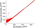
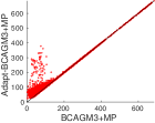
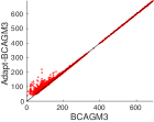
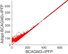
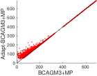
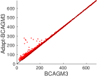
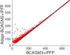
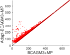
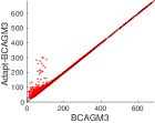
Figure 2: Scatter plots showing matching score of adaptive vs. non-adaptive methods over different datasets.

5.1 Advantages of adaptive methods

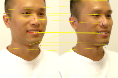
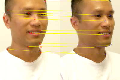
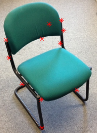
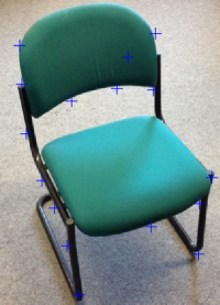
In this section, we compare our adaptive algorithms with the non-adaptive versions. In particular, we conduct our experiments on a realistic dataset [9] which consists of three object classes: face, duck and wine bottle. Each class contains at least 505050 images with different instances.444The dataset consists of 109109109 Face, 505050 Duck, 666666 Wine bottle and is available from [1]. Every image in the dataset is annotated with 101010 ground truth points for matching. We perform our experiments separately on each object class, for which we test all our algorithms on 200020002000 image pairs randomly selected from the same class. In order to make the tasks more difficult, we randomly add to one image several points that are extracted using a SIFT detector. This simulates realistic outlier points resulting from cluttered background in images. In particular, the number of outliers is varied from 00 to 202020 which yields 420042004200 test cases per object class in total. The experimental results are shown in the scatter plot of Fig. 2 where the matching score of the non-adaptive method (x-axis) is plotted against the matching score of the adaptive version (y-axis). One can clearly see that, in all the experiments, the adaptive methods always achieve similar or better matching score than the non-adaptive methods, which confirms the advantage of gradually updating α.𝛼\alpha.

To better understand our algorithms especially in terms of matching accuracy, in the next sections we will compare them with state-of-the-art methods over different datasets. Since the proposed adaptive versions perform better than the non-adaptive approaches, we show below only the performance of the adaptive ones. The appendix provides more detailed comparison between both approaches as well as the fourth-order methods from [36].
Refer to caption
(a)
Refer to caption
(b)
Refer to caption
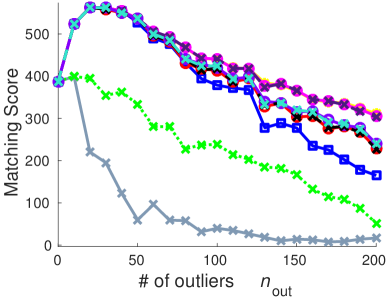
(a) nin=10,σ=0.01formulae-sequencesubscript𝑛𝑖𝑛10𝜎0.01n_{in}=10,\sigma=0.01
Refer to caption
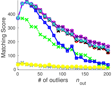
(b) nin=10,σ=0.03,scale=1.5formulae-sequencesubscript𝑛𝑖𝑛10formulae-sequence𝜎0.03scale1.5n_{in}=10,\sigma=0.03,\textrm{scale}=1.5
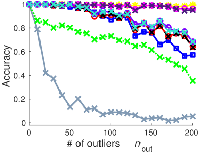
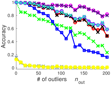
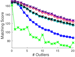
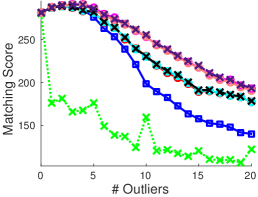
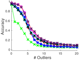
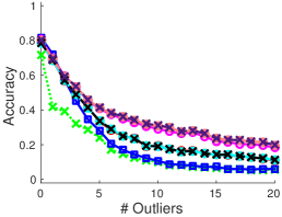
Figure 3: Matching point sets in 2superscript2\mathbb{R}^{2}. The number of outliers is varied from 00 to 200200200. See Fig. 4 for the legend. (Best viewed in color.)
Refer to caption
(a)
Refer to caption
(b)
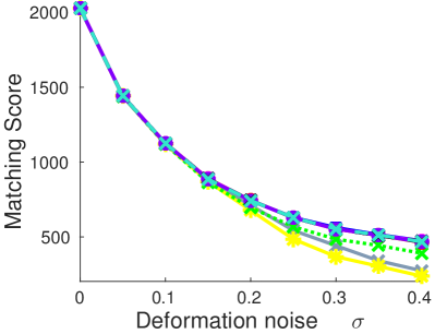
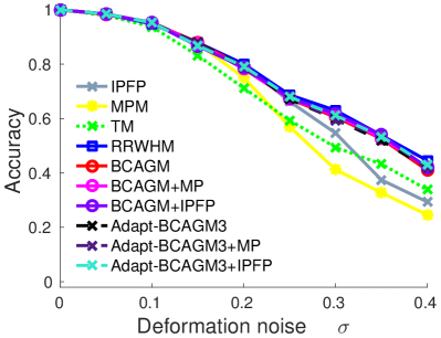
Figure 4: Performance of all algorithms with varying deformation noise. The number of inlier points is fixed as nin=20.subscript𝑛𝑖𝑛20n_{in}=20. (Best viewed in color.)

5.2 Synthetic Dataset

In this section we are trying to match point sets in 2superscript2\mathbb{R}^{2} which is a standard benchmark for testing graph and hypergraph matching methods [12, 25, 14, 28, 50]. We follow a similar procedure as in [12] for the creation of two point sets P𝑃P and Q𝑄Q. In order to create P𝑃P we sample ninsubscript𝑛𝑖𝑛n_{in} inlier points from a Gaussian distribution 𝒩(0,1)𝒩01\mathcal{N}(0,1). These points are then copied to Q𝑄Q and subsequently modified by several operations in the following order: 1) the coordinates of every point are multiplied with a scale factor; 2) additive Gaussian noise 𝒩(0,σ2)𝒩0superscript𝜎2\mathcal{N}(0,\sigma^{2}) is added to every point where σ𝜎\sigma is hereinafter referred to as deformation; 3) on top of that noutsubscript𝑛𝑜𝑢𝑡n_{out} random points, that we refer to as outliers, are added to Q𝑄Q by sampling from 𝒩(0,1)𝒩01\mathcal{N}(0,1). Depending on different scenarios described below, some operations in the above chain might be absent but their order is the same. Based on that, we test all matching algorithms under different changes in the data: outliers, deformation and scaling. In this section, we consider two main settings: outlier and deformation setting. In all plots in this section, each quantitative result was obtained by averaging over 100100100 random trials. The accuracy is computed as the ratio between the number of correct matches and the number of inlier points. We use σs=0.5subscript𝜎𝑠0.5\sigma_{s}=0.5 in the affinity construction for the second-order methods as suggested by [12].

In the outlier setting, we perform two experiments. In the first experiment, we vary the number of outliers from 00 to very challenging 200200200, which is 202020-times more than the number of inliers ninsubscript𝑛𝑖𝑛n_{in}, while σ𝜎\sigma is set to 0.010.010.01 to simulate noise in realistic settings and no scaling is used here (i.e. scale=1.0scale1.0\textrm{scale}=1.0). In the second case, we slightly increase σ𝜎\sigma to 0.030.030.03 and scale all the points in Q𝑄Q by a factor of 1.51.51.5, making the problem more realistic and also much more difficult. This experiment shows the robustness of higher-order methods over second-order ones w.r.t. scale transformations. The results are shown in Fig. 3. Overall, our higher-order algorithms show remarkable tolerance to the number of outliers and significantly outperform previous higher-order as well as second-order methods in terms of both matching score and matching accuracy. The better performance of higher-order approaches shows their robustness against geometric transformations compared to second-order ones. In the first experiment without scaling as shown in Fig. 3 (a), most higher-order methods and MPM perform very well without being deteriorated much by outliers. When the scale change is present in the data as shown in Fig. 3(b), our algorithms significantly outperform the current state-of-the-art. In particular, both MPM and IPFP fail in this case since they use pairwise distance similarities which are clearly not invariant under scaling. Previous higher-order algorithms like RRWHM or TM also show quite rapidly decreasing performance as the number of outliers increases compared to our methods. This experiment also features the difference between two groups of our algorithms, i.e. the ones using MPM as subroutine including BCAGM+MP and Adapt-BCAGM3+MP perform the best in both settings. Thus, one can state that our approach transfers the robustness of MPM as a second-order method to the higher-order case and thus is able to deal with scaling which is difficult for second-order methods.

For the deformation setting, σ𝜎\sigma is varied from 00 to challenging 0.40.40.4 while the number of inliers ninsubscript𝑛𝑖𝑛n_{in} is fixed to 202020. Since we want to test the tolerance of all methods only with respect to deformation, we do not add any outliers nor scale the points in this setting. This type of experiment has been used in previous works [12, 25], where σ𝜎\sigma is varied from 00 to 0.2.0.20.2. Fig. 4 shows the result where our algorithms are quite competitive to RRWHM which has been shown to be robust to deformation before [25]. It is interesting to note that while MPM is very robust against outliers (without scaling), it is outperformed by other methods when the deformation is large. Notably, our algorithms BCAGM+MP and Adapt-BCAGM3+MP using MPM as subroutine are not affected by this slight weakness of MPM.

Considering all experiments in this section, our algorithms outperform or are on par with all previous approaches in terms of robustness to outliers, deformation and scaling. Moreover, our proposed third-order algorithms show on average quite similar performance compared to their fourth-order counterparts [36].
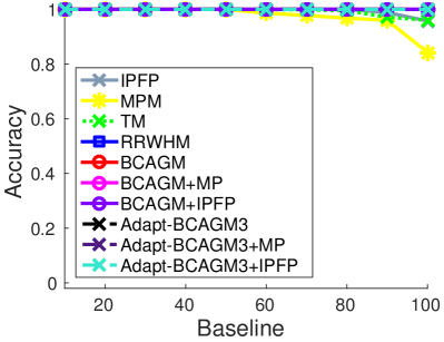
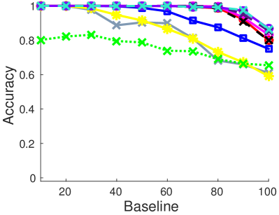
Refer to caption
(a) 30 pts vs. 30 pts
Refer to caption
(b) 20 pts vs. 30 pts
Refer to caption
(c) 10 pts vs. 30 pts
Refer to caption
(d) 10 pts vs. 30 pts
Figure 5: CMU house dataset with different number of points in two images. (Best viewed in color.)

5.3 CMU House Dataset

The CMU house dataset has been widely used in previous work  [10, 25, 15, 50] to evaluate matching algorithms. In this dataset, 30 landmark points are manually tracked over a sequence of 111 images, which are taken from the same object under different view points. In this experiment, “baseline” denotes the distance of the frames in the sequence and thus correlates well with the difficulty to match the corresponding frames.

We match all possible image pairs with “baseline” of 10,20,30,,10010203010010,20,30,\ldots,100 frames and compute the average matching accuracy for each algorithm. The algorithms are evaluated in three settings. In the first experiment, we match 303030 points to 303030 points. Then we make the problem significantly harder by randomly removing points from one image, motivated by a scenario where one has background clutter and thus not all points can be matched. This results in two matching experiments, namely 101010 points to 303030 points, and 202020 points to 303030 points. For the choice of σssubscript𝜎𝑠\sigma_{s} in the affinity tensor for second-order methods, we follow  [10, 50] by setting σs=2500subscript𝜎𝑠2500\sigma_{s}=2500.

The experimental results are shown in Fig. 5. While most algorithms perform rather well on the 303030 to 303030 task, our methods perform significantly better than all other methods in the more difficult tasks, thus showing as for the synthetic datasets that our methods are quite robust to different kinds of noise in the matching problem. Notably, in the 101010 to 303030 task, Adapt-BCAGM3+MP outperforms BCAGM+MP for large baselines.
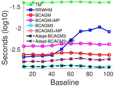
Refer to caption
(a) House
Refer to caption
(b) Willow dataset
Figure 6: Running time of higher-order methods (Best viewed in color.)

5.4 Willow Object Class Dataset
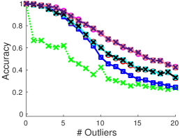
Refer to caption
(a)
Refer to caption
(b)
Refer to caption
(c)
Refer to caption
(a) Face
Refer to caption
(b) Duck
Refer to caption
(c) Winebottle
Figure 7: Matching score and accuracy of higher-order algorithms on Willow Object Dataset [9]. (Best viewed in color.)

In this last experiment we use the Willow Object Class dataset [1] previously introduced in Section 5.1. We use exactly the same setting as in Section 5.1. We test all algorithms on 200020002000 randomly selected image pairs from each object class, where the number of outliers in one image is varied from 00 to 20.2020. For a given number of outliers, we report in Fig. 7 the average performance of all algorithms over all the 200020002000 image pairs. It can be seen that both our third-order and fourth-order methods consistently outperform the state-of-the-art for all the object classes even so the differences are a bit smaller. In particular, for the Duck class, Adapt-BCAGM3+MP performs slightly better than BCAGM+MP even though this is hard to see (see the Appendices for detailed comparisons) because the result has been averaged already over all pairs of images.

5.5 Comparison between third-order methods and fourth-order methods

Synthetic House Face+Duck+Winebottle
Comparison No. Avg(%) No. Avg(%) No. Avg(%)
BCAGM3 >> BCAGM 241 51.9 2 1.5 6277 30.0
BCAGM3 << BCAGM 292 347.0 7 18.5 7130 27.0
BCAGM3 == BCAGM 4567 0.0 1671 0.0 49593 0.0
BCAGM3+IPFP >> BCAGM+IPFP 186 2.4 19 7.5 8960 24.0
BCAGM3+IPFP << BCAGM+IPFP 188 59.5 5 6.9 9834 41.0
BCAGM3+IPFP == BCAGM+IPFP 4726 0.0 1656 0.0 44206 0.0
BCAGM3+MP >> BCAGM+MP 194 43.4 4 12.2 5695 32.0
BCAGM3+MP << BCAGM+MP 243 237.1 6 27.6 7461 56.0
BCAGM3+MP == BCAGM+MP 4663 0.0 1670 0.0 49844 0.0
TABLE I: Comparison between the standard third-order methods (BCAGM3, BCAGM3+ΨΨ\Psi) and the standard fourth-order methods (BCAGM, BCAGM+ΨΨ\Psi [36]) on different datasets. The first column (No.) shows the number of test cases where one algorithm achieves better matching score than the other. The second column (Avg(%)) shows the average performance gain achieved by the better method in each case, which is computed using Eq. (14).
Synthetic House Face+Duck+Winebottle
Comparison No. Avg(%) No. Avg(%) No. Avg(%)
Adapt-BCAGM3 >> Adapt-BCAGM 269 47.2 3 1.6 6717 28.0
Adapt-BCAGM3 << Adapt-BCAGM 239 51.6 3 20.3 5621 23.0
Adapt-BCAGM3 == Adapt-BCAGM 4592 0.0 1674 0.0 50662 0.0
Adapt-BCAGM3+IPFP >> Adapt-BCAGM+IPFP 207 2.3 20 6.9 10774 21.0
Adapt-BCAGM3+IPFP << Adapt-BCAGM+IPFP 109 55.6 3 1.9 6318 26.0
Adapt-BCAGM3+IPFP == Adapt-BCAGM+IPFP 4784 0.0 1657 0.0 45908 0.0
Adapt-BCAGM3+MP >> Adapt-BCAGM+MP 217 39.0 4 12.2 6311 29.0
Adapt-BCAGM3+MP << Adapt-BCAGM+MP 177 59.0 4 10.4 5603 26.0
Adapt-BCAGM3+MP == Adapt-BCAGM+MP 4706 0.0 1672 0.0 51086 0.0
TABLE II: Comparison between the adaptive third-order methods (Adapt-BCAGM3, Adapt-BCAGM3+ΨΨ\Psi) and the adaptive fourth-order methods (Adapt-BCAGM, Adapt-BCAGM+ΨΨ\Psi) on different datasets. The first column (No.) shows the number of test cases where one algorithm achieves better matching score than the other. The second column (Avg(%)) shows the average performance gain achieved by the better method in each case, which is computed using Eq. (14).

This section presents a detailed comparison of our third-order approaches and fourth-order approaches. In particular, we first compare the non-adaptive third-order algorithms (Algorithm 1 and Algorithm 2) to their non-adaptive fourth-order counterparts [36]. Second, we extend the adaptive scheme derived for third-order tensors in Section 3.3 to fourth-order tensors, and denote the corresponding adaptive fourth-order algorithms as Adapt-BCAGM, Adapt-BCAGM+IPFP and Adapt-BCAGM+MP with the same notation as before. We then compare these algorithms with the adaptive third-order methods from Algorithm 3 and Algorithm 4. The purpose is to test for advantages and disadvantages of third-order approaches versus fourth-order ones under both settings – with and without adaptive updates.

For each pair of algorithms, we report in Table I the number of test cases where one algorithm performs better than the other one in terms of matching score and how much improvement it achieves on average over the other method for the cases where the performance is not equal. More precisely, let fisubscript𝑓𝑖f_{i} and gisubscript𝑔𝑖g_{i} be the matching score of BCAGM3 and BCAGM respectively on the Synthetic dataset. Then “BCAGM3 >> BCAGM” denotes the cases where BCAGM3 achieves a better objective value than BCAGM, and we report this number in the first column (No.), that is, |{i|fi>gi}|,|𝑖subscript𝑓𝑖subscript𝑔𝑖\left|\left\{i\mathrel{\left|\vphantom{if_{i}>g_{i}}\right.}f_{i}>g_{i}\right\}\right|, and the average performance gain in the second column (Avg(%)), that is,

1|{i|fi>gi}|i:fi>gifigigi.1|𝑖subscript𝑓𝑖subscript𝑔𝑖subscript:𝑖subscript𝑓𝑖subscript𝑔𝑖subscript𝑓𝑖subscript𝑔𝑖subscript𝑔𝑖\frac{1}{\left|\left\{i\mathrel{\left|\vphantom{if_{i}>g_{i}}\right.}f_{i}>g_{i}\right\}\right|}\sum\limits_{i:f_{i}>g_{i}}\frac{f_{i}-g_{i}}{g_{i}}. (14)

Table I shows that the standard fourth-order algorithms [36] have a better overall performance than the standard third-order ones in terms of matching score. However, the differences are minor and obtaining better matching score does not necessarily imply the same for matching accuracy, especially when the ground truth is not a global optimum of the hypergraph matching problem. Fig. 7 (a) shows an example of this phenomenon where third-order methods achieve better matching score than the fourth-order algorithms but their matching accuracy is very similar.

Table II shows the same kind of comparison but for the adaptive schemes. One can see that the situation has changed as the adaptive third-order schemes win more frequently over their fourth-order counterparts. Again, the differences are minor. While on the synthetic dataset the adaptive fourth-order methods perform better, on the real dataset, it is the opposite.

All in all, one can state that the standard fourth-order algorithms are better than the standard third-order approaches in terms of achieving better matching score. This indicates potential benefits of using fourth-order tensors as well as the lifting step as done in [36]. However, the differences between the adaptive third- and fourth-order methods are negligible and are slightly on the side of the adaptive third-order methods. As the third-order methods are two times faster (see next section), our recommendation is to use the adaptive third-order methods in practice.

5.6 Running time

Fig. 6 shows the running time of all hypergraph matching algorithms. All our methods achieve competitive/smaller running time than the state-of-the-art, in particular, they are 444 to 161616 times faster than TM while being competitive to RRWHM in case of BCAGM3+MP or up to two times faster in case of BCAGM3 and Adapt-BCAGM3. It can also be seen that the proposed third-order approaches are two times faster than their fourth-order counterparts on average. Further experimental results on the running time of all higher-order algorithms can be found in Tab. VI, Tab. VII and Tab. VIII in the appendix.

6 Demo of matching results

We show in this section a demo matching on realistic images. Different from the previous sections, we run a SIFT detector on two realistic images, hence, there might be outliers in both point sets. Since each point on one image might not have a corresponding point on the other image, the matching task becomes more difficult. Fig. 8 shows the matching results. Our algorithms achieve more reasonable matches than the previous higher-order approaches while also achieving consistently better matching score than the others. Further examples can be found in the appendix.

7 Conclusion and Outlook

In this work, we present a new optimization framework for hypergraph matching based on a multilinear reformulation. In particular, we extend our theory from fourth-order tensors [36] to third-order tensors, proving under mild conditions the equivalence between the maximization of a third-order multilinear form and the maximization of its associated score function. Based on that, we propose Algorithm 1 and Algorithm 2 which both maximize the third-order multilinear form directly over the set of assignment constraints. These algorithms share the same attributes with their fourth-order counterparts [36] in the sense that they achieve monotonic ascent in the original score function directly on the set of assignment matrices, and both converge to a homogeneous solution in a finite number of steps. Furthermore, we provide several sufficient conditions, weaker than the convexity constraint used in [36], to ensure the equivalence between the optimization problems. We also propose two adaptive schemes which yield slight improvements over the standard approaches. Overall, our algorithms, including the fourth-order and the third-order ones, not only achieve superior performance in terms of matching score but also yield competitive or significantly better matching accuracy than previous work. This holds even when there are a large number of outliers, deformation, scaling or other form of noise in the data. Moreover, our methods are competitive or better in terms of runtime compared to previous work. Our new adaptive third-order methods are competitive to the corresponding adaptive fourth-order ones but are on average two times faster and thus we recommend them for usage in practice.
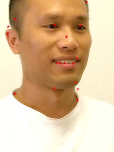
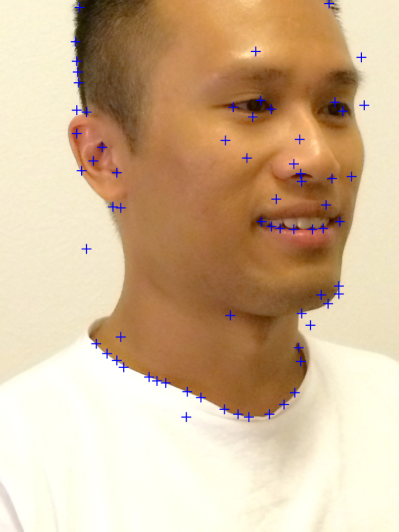
Refer to caption
(a) Image 1
Refer to caption
(b) Image 2
Refer to caption
(c) TM[15] (363)
Refer to caption
(d) RRWHM[25] (441)
Refer to caption
(e) BCAGM[36] (599)
Refer to caption
(f) BCAGM+MP[36] (600)
Refer to caption
(g) Adapt-BCAGM3 (600)
Refer to caption
(h) Adapt-BCAGM3+MP (600)
Figure 8: Demo of matching results. Matching score is reported for each method. (Best viewed in color.)

For future work it might be interesting to go beyond injective mappings which require every point on one image to be mapped to exactly one point in the second image. Non-injective mappings are of interest if not all points need to be matched as for instance when outliers are present on both sides [40, 30]. Our Theorem 3.3 allows the use of new constraint sets reflecting non-injective mappings, which is an interesting topic of further research. Another possible generalization is to go beyond third-order (this paper) or fourth-order [36] hypergraphs which would require a generalization of Theorem 3.3. At the moment it is unclear to us if this is possible.

Acknowledgments

This work has been supported by the ERC grant NOLEPRO. We sincerely thank the reviewers for their helpful comments and Cristian Caloian for helping us to correct grammatical mistakes.

References

  • [1] http://www.di.ens.fr/willow/research/graphlearning/.
  • [2] C. Arora and A. Globerson. Higher order matching for consistent multiple target tracking. In ICCV, 2013.
  • [3] S. Arya, D. M. Mount, N. S. Netanyahu, R. Silverman, and A. Wu. An optimal algorithm for approximate nearest neighbor searching. Journal of the ACM, 45:891–923, 1998.
  • [4] E. Boros and P. L. Hammer. Pseudo-boolean optimization. Discrete Applied Mathematics, 123:155–225, 2002.
  • [5] R. E. Burkhard, M. Dell’Amico, and S. Martello. Assignment problems. SIAM, Philadelphia, 2012.
  • [6] M. Carcassoni and E. R. Hancock. Spectral correspondence for point pattern matching. Pattern Recognition, 36:193–204, 2003.
  • [7] Z.-Q. Cheng, Y. Chen, M. R.R., Y.-K. Lai, and A. Wang. Supermatching: Feature matching using supersymmetric geometric constraints. IEEE Transactions on Visualization and Computer Graphics, 10:1885–1894, 2012.
  • [8] M. Chertok and Y. Keller. Efficient high order matching. PAMI, 32:2205–2215, 2010.
  • [9] M. Cho, K. Alahari, and J. Ponce. Learning graphs to match. In ICCV, 2013.
  • [10] M. Cho, J. Lee, and K. M. Lee. Reweighted random walks for graph matching. In ECCV, 2010.
  • [11] M. Cho and K. M. Lee. Progressive graph matching: Making a move of graphs via probabilistic voting. In CVPR, 2012.
  • [12] M. Cho, J. Sun, O. Duchenne, and J. Ponce. Finding matches in a haystack: A max-pooling strategy for graph matching in the presence of outliers. In CVPR, 2014.
  • [13] D. Conte, P. Foggia, C. Sansone, and M. Vento. Thirty years of graph matching. PAMI, 18:265–298, 2004.
  • [14] T. Cour, P. Srinivasan, and J. Shi. Balanced graph matching. In NIPS, 2007.
  • [15] O. Duchenne, F. Bach, I. Kweon, and J. Ponce. A tensor-based algorithm for high-order graph matching. PAMI, 33:2383–2395, 2011.
  • [16] O. Duchenne, A. Joulin, and J. Ponce. A graph-matching kernel for object categorization. In ICCV, 2011.
  • [17] A. Filatov, A. Gitis, and I. Kil. Graph-based handwritten digit string recognition. In Proc. Third Int’l Conf. Document Analysis and Recognition, 1995.
  • [18] P. Foggia, G. Percannella, and M. Vento. Graph matching and learning in pattern recognition in the last 10 years. Pattern Recognition and Artificial Intelligence, 28, 2014.
  • [19] R. Hartley and A. Zisserman. Tutorial i: The algebraic approach to invariance. In ESPRIT Workshop, 1994.
  • [20] J. Hays, M. Leordeanu, A. A. Efros, and Y. Liu. Discovering texture regularity as a higher-order correspondence problem. In ECCV, 2006.
  • [21] J. E. Hopcroft and J. K. Wong. Linear time algorithm for isomorphism of planar graphs (preliminary report). Proc. Sixth Ann. ACM Symp. Theory of Computing, pages 172–184, 1974.
  • [22] V. Kolmogorov and C. Rother. Minimizing nonsubmodular functions with graph cuts-a review. PAMI, 29:1274–1279, 2007.
  • [23] H. W. Kuhn. The hungarian method for the assignment problem. Naval Research Logistics Quarterly, 2:83–97, 1955.
  • [24] J. Lee, M. Cho, and K. M. Lee. A graph matching algorithm using data-driven markov chain monte carlo sampling. In ICPR, 2010.
  • [25] J. Lee, M. Cho, and K. M. Lee. Hyper-graph matching via reweighted random walks. In CVPR, 2011.
  • [26] R. Lee and J. Liu. An oscillatory elastic graph matching model for recognition of offline handwritten chinese characters. In Knowledge-Based Intelligent Information Engineering Systems, 1999.
  • [27] M. Leordeanu and M. Hebert. A spectral technique for correspondence problems using pairwise constraints. In ICCV, 2005.
  • [28] M. Leordeanu and M. Hebert. Unsupervised learning for graph matching. In CVPR, 2009.
  • [29] M. Leordeanu, M. Hebert, and R. Sukthankar. An integer projected fixed point method for graph matching and map inference. In NIPS, 2009.
  • [30] W. Lian and L. Zhang. Point matching in the presence of outliers in both point sets: A concave optimization approach. In CVPR, 2014.
  • [31] Z.-Y. Liu, H. Qiao, and L. Xu. An extended path following algorithm for graph-matching problem. PAMI, 34:1451–1456, 2012.
  • [32] D. G. Lowe. Object recognition from local scale-invariant features. In ICCV, 1999.
  • [33] B. Luo and E. Hancock. Alignment and correspondence using singular value decomposition. Advances in Pattern Recognition, 1876:226–235, 2000.
  • [34] J. Maciel and J. P. Costeira. A global solution to sparse correspondence problems. PAMI, 25:187–199, 2003.
  • [35] J. L. Mundy, A. Zisserman, and D. Forsyth. Applications of Invariance in Computer Vision. Springer, 1993.
  • [36] Q. Nguyen, A. Gautier, and M. Hein. A flexible tensor block coordinate ascent scheme for hypergraph matching. In CVPR, 2015.
  • [37] C. Schellewald and C. Schnörr. Probabilistic subgraph matching based on convex relaxation. In EMMCVPR, 2005.
  • [38] A. Sharma, R. Horaud, J. Cech, and E. Boyer. Topologically- robust 3d shape matching based on diffusion geometry and seed growing. In CVPR, 2011.
  • [39] R. Singh, J. Xu, and B. Berger. Pairwise global alignment of protein interaction networks by matching neighborhood topology. Proc. 11th Int’l Conf. Research in Computational Molecular Biology, pages 16–31, 2007.
  • [40] Y. Suh and K. M. Lee. Subgraph matching using compactness prior for robust feature correspondence. In CVPR, 2015.
  • [41] W. Taylor. Protein structure comparison using bipartite graph matching and its application to protein structure classification. Molecular and Cellular Proteomics, 1:334–339, 2002.
  • [42] L. Torresani, V. Kolmogorov, and C. Rother. Feature correspondence via graph matching: Models and global optimization. In ECCV, 2008.
  • [43] H. F. Wang and E. R. Hancock. Correspondence matching using kernel principal components analysis and label consistency constraints. Pattern Recognition, 39:1012–1025, 2006.
  • [44] Y. Wang, F. Makedon, and J. Ford. A bipartite graph matching framework for finding correspondences between structural elements in two proteins. In Proc. IEEE 26th Ann. Int’l Conf. Eng. in Medicine and Biology Society, 2004.
  • [45] J. Yan, C. Zhang, H. Zha, W. Liu, X. Yang, and S. M. Chu. Discrete hyper-graph matching. In CVPR, 2015.
  • [46] M. Zaslavskiy, F. Bach, and J. Vert. A path following algorithm for the graph matching problem. PAMI, 31:2227–2242, 2009.
  • [47] R. Zass and A. Shashua. Probabilistic graph and hypergraph matching. In CVPR, 2008.
  • [48] Y. Zeng, C. Wang, Y. Wang, X. Gu, D. Samaras, and N. Paragios. Dense non-rigid surface registration using high-order graph matching. In CVPR, 2010.
  • [49] F. Zhou and F. De la Torre. Factorized graph matching. In CVPR, 2012.
  • [50] F. Zhou and F. De la Torre. Deformable graph matching. In CVPR, 2013.
[Uncaptioned image] Quynh Nguyen is currently a PhD student in the Machine Learning Group of Saarland University. He received his BSc degree in Information Technology from Vietnam National University in Hanoi in 2011. In 2014, he got his Msc degree in Computer Science from Saarland University through the support of the IMPRS for Computer Science in Saarbruecken, Germany. His research interests are in machine learning, optimization and computer vision.
[Uncaptioned image] Francesco Tudisco is a Postdoctoral fellow in Mathematics at Saarland University, within the Machine Learning Group. He received his diploma and his Ph.D. in Mathematics from the University of Rome ”Tor Vergata”. His main scientific interests include Operator Theory, Numerical Linear Algebra, Network Analysis and Numerical Optimization.
[Uncaptioned image] Antoine Gautier is a PhD student in the machine learning group of Saarland university since 2014. He received a B.Sc. (2011) and a M.Sc. (2013) degree in applied mathematics from EPFL, Lausanne, Switzerland. In 2010, he spent a year at the Humboldt university of Berlin for an Erasmus exchange. His main research interests are higher-order structures, optimization, nonlinear spectral theory and their applications in computational science.
[Uncaptioned image] Matthias Hein is professor of mathematics and computer science at Saarland University. He received his diploma in physics from the University of Tübingen in 2002 and his PhD in computer science from the University of Darmstadt in 2005. His research interests are in machine learning, statistics and optimization and the application of machine learning to problems in bioinformatics, computer vision and other fields in computer science and the natural sciences.

Appendix A

Theorem 3.3

Let Dn𝐷superscript𝑛D\subset\mathbb{R}^{n} be a compact set, F:n×n×n:Fsuperscript𝑛superscript𝑛superscript𝑛\textit{F}:\mathbb{R}^{n}\times\mathbb{R}^{n}\times\mathbb{R}^{n}\to\mathbb{R} a symmetric third-order multilinear form and S:n:𝑆superscript𝑛S:\mathbb{R}^{n}\to\mathbb{R} the associated third-order score function such that S(𝐱)=F(𝐱,𝐱,𝐱),𝑆𝐱𝐹𝐱𝐱𝐱S(\mathbf{x})=F(\mathbf{x},\mathbf{x},\mathbf{x}), then we have the following chain of implications: 1) \Rightarrow 2) \Rightarrow 3) \Rightarrow 4).

  1. 1.

    2S(𝐱)superscript2𝑆𝐱\nabla^{2}S(\mathbf{x}) is positive semidefinite for all 𝐱D.𝐱𝐷\mathbf{x}\in D.

  2. 2.

    F(𝐱,𝐲𝐳,𝐲𝐳)0F𝐱𝐲𝐳𝐲𝐳0\textit{F}(\mathbf{x},\mathbf{y}-\mathbf{z},\mathbf{y}-\mathbf{z})\geq 0 for all 𝐱,𝐲,𝐳D.𝐱𝐲𝐳𝐷\mathbf{x},\mathbf{y},\mathbf{z}\in D.

  3. 3.

    It holds for all 𝐱,𝐲,𝐳D𝐱𝐲𝐳𝐷\mathbf{x},\mathbf{y},\mathbf{z}\in D

    F(𝐱,𝐲,𝐳)max𝐮{𝐱,𝐲,𝐳}F(𝐮,𝐮,𝐮).F𝐱𝐲𝐳subscriptmax𝐮𝐱𝐲𝐳F𝐮𝐮𝐮\textit{F}(\mathbf{x},\mathbf{y},\mathbf{z})\leq\mathop{\rm max}\nolimits\limits_{\mathbf{u}\in\{\mathbf{x},\mathbf{y},\mathbf{z}\}}\textit{F}(\mathbf{u},\mathbf{u},\mathbf{u}).
  4. 4.

    The optimization of the multilinear form is equivalent to the optimization of its associated score function

    max𝐱,𝐲,𝐳DF(𝐱,𝐲,𝐳)=max𝐱,𝐲DF(𝐱,𝐱,𝐲)=max𝐱DF(𝐱,𝐱,𝐱).subscriptmax𝐱𝐲𝐳𝐷F𝐱𝐲𝐳subscriptmax𝐱𝐲𝐷F𝐱𝐱𝐲subscriptmax𝐱𝐷F𝐱𝐱𝐱\!\!\!\!\mathop{\rm max}\nolimits\limits_{\mathbf{x},\mathbf{y},\mathbf{z}\in D}\textit{F}(\mathbf{x},\mathbf{y},\mathbf{z})=\mathop{\rm max}\nolimits\limits_{\mathbf{x},\mathbf{y}\in D}\textit{F}(\mathbf{x},\mathbf{x},\mathbf{y})=\mathop{\rm max}\nolimits\limits_{\mathbf{x}\in D}\textit{F}(\mathbf{x},\mathbf{x},\mathbf{x}).
Proof:
  • 1)2):1)\implies 2): We first recall the definition of the score function as

    S(𝐱)=F(𝐱,𝐱,𝐱)=i,j,k=1nijk𝐱i𝐱j𝐱k.𝑆𝐱F𝐱𝐱𝐱superscriptsubscript𝑖𝑗𝑘1𝑛subscript𝑖𝑗𝑘subscript𝐱𝑖subscript𝐱𝑗subscript𝐱𝑘S(\mathbf{x})=\textit{F}(\mathbf{x},\mathbf{x},\mathbf{x})=\sum_{i,j,k=1}^{n}\mathcal{F}_{ijk}{\color[rgb]{0,0,0}\definecolor[named]{pgfstrokecolor}{rgb}{0,0,0}\pgfsys@color@gray@stroke{0}\pgfsys@color@gray@fill{0}\mathbf{x}_{i}\mathbf{x}_{j}\mathbf{x}_{k}}.

    One can compute the Hessian of S𝑆S at 𝐱𝐱\mathbf{x} as follows

    (2S(𝐱))ij=6k=1nijk𝐱ki,j=1,,n.formulae-sequencesubscriptsuperscript2𝑆𝐱𝑖𝑗6superscriptsubscript𝑘1𝑛subscript𝑖𝑗𝑘subscript𝐱𝑘for-all𝑖𝑗1𝑛\left(\nabla^{2}S(\mathbf{x})\right)_{ij}=6\sum_{k=1}^{n}\mathcal{F}_{ijk}\mathbf{x}_{k}\quad\forall\,i,j=1,\ldots,n.

    Using our notation, the Hessian can be rewritten as

    2S(𝐱)=6F(𝐱,,).superscript2𝑆𝐱6F𝐱\nabla^{2}S(\mathbf{x})=6\,\textit{F}(\mathbf{x},\,\cdot\,,\,\cdot\,).

    The Hessian 2S(𝐱)superscript2𝑆𝐱\nabla^{2}S(\mathbf{x}) is is positive semidefinite for all 𝐱D𝐱𝐷\mathbf{x}\in D if and only if 𝐭,2S(𝐱)𝐭0𝐭superscript2𝑆𝐱𝐭0\left\langle\mathbf{t},\nabla^{2}S(\mathbf{x})\,\mathbf{t}\right\rangle\geq 0 for all 𝐱D,𝐭nformulae-sequence𝐱𝐷𝐭superscript𝑛\mathbf{x}\in D,\mathbf{t}\in\mathbb{R}^{n}, which is equivalent to F(𝐱,𝐭,𝐭)0F𝐱𝐭𝐭0\textit{F}(\mathbf{x},\mathbf{t},\mathbf{t})\geq 0 for all 𝐱D,𝐭nformulae-sequence𝐱𝐷𝐭superscript𝑛\mathbf{x}\in D,\mathbf{t}\in\mathbb{R}^{n} and thus,

    F(𝐱,𝐲𝐳,𝐲𝐳)0𝐱,𝐲,𝐳D.formulae-sequenceF𝐱𝐲𝐳𝐲𝐳0for-all𝐱𝐲𝐳𝐷\textit{F}(\mathbf{x},\mathbf{y}-\mathbf{z},\mathbf{y}-\mathbf{z})\geq 0\quad\forall\,\mathbf{x},\mathbf{y},\mathbf{z}\in D.
  • 2)3):2)\implies 3): Given 𝐱,𝐲,𝐳D𝐱𝐲𝐳𝐷\mathbf{x},\mathbf{y},\mathbf{z}\in D, the statement 2) implies that F(𝐱,𝐱𝐲,𝐱𝐲)0F𝐱𝐱𝐲𝐱𝐲0\textit{F}(\mathbf{x},\mathbf{x}-\mathbf{y},\mathbf{x}-\mathbf{y})\geq 0 and F(𝐲,𝐱𝐲,𝐱𝐲)0F𝐲𝐱𝐲𝐱𝐲0\textit{F}(\mathbf{y},\mathbf{x}-\mathbf{y},\mathbf{x}-\mathbf{y})\geq 0, thus,

    00\displaystyle 0 \displaystyle\leq F(𝐱,𝐱𝐲,𝐱𝐲)+F(𝐲,𝐱𝐲,𝐱𝐲)F𝐱𝐱𝐲𝐱𝐲F𝐲𝐱𝐲𝐱𝐲\displaystyle\textit{F}(\mathbf{x},\mathbf{x}-\mathbf{y},\mathbf{x}-\mathbf{y})+\textit{F}(\mathbf{y},\mathbf{x}-\mathbf{y},\mathbf{x}-\mathbf{y})
    =\displaystyle= F(𝐱,𝐱,𝐱)+F(𝐲,𝐲,𝐲)F(𝐱,𝐱,𝐲)F(𝐱,𝐲,𝐲)F𝐱𝐱𝐱F𝐲𝐲𝐲F𝐱𝐱𝐲F𝐱𝐲𝐲\displaystyle\textit{F}(\mathbf{x},\mathbf{x},\mathbf{x})+\textit{F}(\mathbf{y},\mathbf{y},\mathbf{y})-\textit{F}(\mathbf{x},\mathbf{x},\mathbf{y})-\textit{F}(\mathbf{x},\mathbf{y},\mathbf{y})

    By switching the roles of 𝐱,𝐲,𝐳𝐱𝐲𝐳\mathbf{x},\mathbf{y},\mathbf{z}, we can derive the following inequalities

    F(𝐱,𝐱,𝐲)+F(𝐱,𝐲,𝐲)F𝐱𝐱𝐲F𝐱𝐲𝐲\displaystyle\textit{F}(\mathbf{x},\mathbf{x},\mathbf{y})+\textit{F}(\mathbf{x},\mathbf{y},\mathbf{y}) \displaystyle\leq F(𝐱,𝐱,𝐱)+F(𝐲,𝐲,𝐲)F𝐱𝐱𝐱F𝐲𝐲𝐲\displaystyle\textit{F}(\mathbf{x},\mathbf{x},\mathbf{x})+\textit{F}(\mathbf{y},\mathbf{y},\mathbf{y})
    F(𝐱,𝐱,𝐳)+F(𝐱,𝐳,𝐳)F𝐱𝐱𝐳F𝐱𝐳𝐳\displaystyle\textit{F}(\mathbf{x},\mathbf{x},\mathbf{z})+\textit{F}(\mathbf{x},\mathbf{z},\mathbf{z}) \displaystyle\leq F(𝐱,𝐱,𝐱)+F(𝐳,𝐳,𝐳)F𝐱𝐱𝐱F𝐳𝐳𝐳\displaystyle\textit{F}(\mathbf{x},\mathbf{x},\mathbf{x})+\textit{F}(\mathbf{z},\mathbf{z},\mathbf{z})
    F(𝐲,𝐲,𝐳)+F(𝐲,𝐳,𝐳)F𝐲𝐲𝐳F𝐲𝐳𝐳\displaystyle\textit{F}(\mathbf{y},\mathbf{y},\mathbf{z})+\textit{F}(\mathbf{y},\mathbf{z},\mathbf{z}) \displaystyle\leq F(𝐲,𝐲,𝐲)+F(𝐳,𝐳,𝐳)F𝐲𝐲𝐲F𝐳𝐳𝐳\displaystyle\textit{F}(\mathbf{y},\mathbf{y},\mathbf{y})+\textit{F}(\mathbf{z},\mathbf{z},\mathbf{z})

    Summing up these equations gives us

    F(𝐱,𝐱,𝐲)+F(𝐱,𝐲,𝐲)+F(𝐱,𝐱,𝐳)+F𝐱𝐱𝐲F𝐱𝐲𝐲limit-fromF𝐱𝐱𝐳\displaystyle\textit{F}(\mathbf{x},\mathbf{x},\mathbf{y})+\textit{F}(\mathbf{x},\mathbf{y},\mathbf{y})+\textit{F}(\mathbf{x},\mathbf{x},\mathbf{z})+ (15)
    F(𝐱,𝐳,𝐳)+F(𝐲,𝐲,𝐳)+F(𝐲,𝐳,𝐳)F𝐱𝐳𝐳F𝐲𝐲𝐳F𝐲𝐳𝐳\displaystyle\textit{F}(\mathbf{x},\mathbf{z},\mathbf{z})+\textit{F}(\mathbf{y},\mathbf{y},\mathbf{z})+\textit{F}(\mathbf{y},\mathbf{z},\mathbf{z})
    \displaystyle\leq 2F(𝐱,𝐱,𝐱)+2F(𝐲,𝐲,𝐲)+2F(𝐳,𝐳,𝐳).2F𝐱𝐱𝐱2F𝐲𝐲𝐲2F𝐳𝐳𝐳\displaystyle 2\textit{F}(\mathbf{x},\mathbf{x},\mathbf{x})+2\textit{F}(\mathbf{y},\mathbf{y},\mathbf{y})+2\textit{F}(\mathbf{z},\mathbf{z},\mathbf{z}).

    The statement 2) also implies the following inequalities

    0F(𝐱,𝐲𝐳,𝐲𝐳)0F𝐱𝐲𝐳𝐲𝐳\displaystyle 0\leq\textit{F}(\mathbf{x},\mathbf{y}-\mathbf{z},\mathbf{y}-\mathbf{z})
    0F(𝐲,𝐳𝐱,𝐳𝐱)0F𝐲𝐳𝐱𝐳𝐱\displaystyle 0\leq\textit{F}(\mathbf{y},\mathbf{z}-\mathbf{x},\mathbf{z}-\mathbf{x})
    0F(𝐳,𝐱𝐲,𝐱𝐲)0F𝐳𝐱𝐲𝐱𝐲\displaystyle 0\leq\textit{F}(\mathbf{z},\mathbf{x}-\mathbf{y},\mathbf{x}-\mathbf{y})

    which can be expanded as

    2F(𝐱,𝐲,𝐳)F(𝐱,𝐲,𝐲)+F(𝐱,𝐳,𝐳)2F𝐱𝐲𝐳F𝐱𝐲𝐲F𝐱𝐳𝐳\displaystyle 2\textit{F}(\mathbf{x},\mathbf{y},\mathbf{z})\leq\textit{F}(\mathbf{x},\mathbf{y},\mathbf{y})+\textit{F}(\mathbf{x},\mathbf{z},\mathbf{z})
    2F(𝐲,𝐳,𝐱)F(𝐲,𝐳,𝐳)+F(𝐲,𝐱,𝐱)2F𝐲𝐳𝐱F𝐲𝐳𝐳F𝐲𝐱𝐱\displaystyle 2\textit{F}(\mathbf{y},\mathbf{z},\mathbf{x})\leq\textit{F}(\mathbf{y},\mathbf{z},\mathbf{z})+\textit{F}(\mathbf{y},\mathbf{x},\mathbf{x})
    2F(𝐳,𝐱,𝐲)F(𝐳,𝐱,𝐱)+F(𝐳,𝐲,𝐲).2F𝐳𝐱𝐲F𝐳𝐱𝐱F𝐳𝐲𝐲\displaystyle 2\textit{F}(\mathbf{z},\mathbf{x},\mathbf{y})\leq\textit{F}(\mathbf{z},\mathbf{x},\mathbf{x})+\textit{F}(\mathbf{z},\mathbf{y},\mathbf{y}).

    By summing up these inequalities and taking into account the symmetry of F, one obtains

    6F(𝐱,𝐲,𝐳)6F𝐱𝐲𝐳\displaystyle 6\,\textit{F}(\mathbf{x},\mathbf{y},\mathbf{z}) \displaystyle\leq F(𝐱,𝐲,𝐲)+F(𝐱,𝐳,𝐳)+F(𝐲,𝐱,𝐱)+F𝐱𝐲𝐲F𝐱𝐳𝐳limit-fromF𝐲𝐱𝐱\displaystyle\textit{F}(\mathbf{x},\mathbf{y},\mathbf{y})+\textit{F}(\mathbf{x},\mathbf{z},\mathbf{z})+\textit{F}(\mathbf{y},\mathbf{x},\mathbf{x})+ (16)
    F(𝐲,𝐳,𝐳)+F(𝐳,𝐱,𝐱)+F(𝐳,𝐲,𝐲).F𝐲𝐳𝐳F𝐳𝐱𝐱F𝐳𝐲𝐲\displaystyle\textit{F}(\mathbf{y},\mathbf{z},\mathbf{z})+\textit{F}(\mathbf{z},\mathbf{x},\mathbf{x})+\textit{F}(\mathbf{z},\mathbf{y},\mathbf{y}).

    Combining (15) and (16) to achieve

    6F(𝐱,𝐲,𝐳)2F(𝐱,𝐱,𝐱)+2F(𝐲,𝐲,𝐲)+2F(𝐳,𝐳,𝐳),6F𝐱𝐲𝐳2F𝐱𝐱𝐱2F𝐲𝐲𝐲2F𝐳𝐳𝐳\displaystyle 6\,\textit{F}(\mathbf{x},\mathbf{y},\mathbf{z})\leq 2\textit{F}(\mathbf{x},\mathbf{x},\mathbf{x})+2\textit{F}(\mathbf{y},\mathbf{y},\mathbf{y})+2\textit{F}(\mathbf{z},\mathbf{z},\mathbf{z}),

    which implies

    F(𝐱,𝐲,𝐳)max{F(𝐱,𝐱,𝐱),F(𝐲,𝐲,𝐲),F(𝐳,𝐳,𝐳)}.F𝐱𝐲𝐳maxF𝐱𝐱𝐱F𝐲𝐲𝐲F𝐳𝐳𝐳\displaystyle\textit{F}(\mathbf{x},\mathbf{y},\mathbf{z})\leq\mathop{\rm max}\nolimits\{\textit{F}(\mathbf{x},\mathbf{x},\mathbf{x}),\textit{F}(\mathbf{y},\mathbf{y},\mathbf{y}),\textit{F}(\mathbf{z},\mathbf{z},\mathbf{z})\}.
  • 3)4):3)\implies 4): From the statement 3)

    F(𝐱,𝐲,𝐳)max𝐮{𝐱,𝐲,𝐳}F(𝐮,𝐮,𝐮),F𝐱𝐲𝐳subscriptmax𝐮𝐱𝐲𝐳F𝐮𝐮𝐮\textit{F}(\mathbf{x},\mathbf{y},\mathbf{z})\leq\mathop{\rm max}\nolimits\limits_{\mathbf{u}\in\{\mathbf{x},\mathbf{y},\mathbf{z}\}}\textit{F}(\mathbf{u},\mathbf{u},\mathbf{u}),

    one takes the maximum of both sides over D𝐷D to achieve

    max𝐱,𝐲,𝐳DF(𝐱,𝐲,𝐳)subscriptmax𝐱𝐲𝐳𝐷F𝐱𝐲𝐳\displaystyle\mathop{\rm max}\nolimits\limits_{\mathbf{x},\mathbf{y},\mathbf{z}\in D}\textit{F}(\mathbf{x},\mathbf{y},\mathbf{z}) \displaystyle\leq max𝐱,𝐲,𝐳D{max𝐮{𝐱,𝐲,𝐳}F(𝐮,𝐮,𝐮)}subscriptmax𝐱𝐲𝐳𝐷subscriptmax𝐮𝐱𝐲𝐳F𝐮𝐮𝐮\displaystyle\mathop{\rm max}\nolimits\limits_{\mathbf{x},\mathbf{y},\mathbf{z}\in D}\left\{\mathop{\rm max}\nolimits\limits_{\mathbf{u}\in\{\mathbf{x},\mathbf{y},\mathbf{z}\}}\textit{F}(\mathbf{u},\mathbf{u},\mathbf{u})\right\}
    =\displaystyle= max𝐱DF(𝐱,𝐱,𝐱).subscriptmax𝐱𝐷F𝐱𝐱𝐱\displaystyle\mathop{\rm max}\nolimits\limits_{\mathbf{x}\in D}\textit{F}(\mathbf{x},\mathbf{x},\mathbf{x}).

    However, it holds for any compact set Dn𝐷superscript𝑛D\subset\mathbb{R}^{n} that

    max𝐱,𝐲,𝐳DF(𝐱,𝐲,𝐳)max𝐱,𝐲DF(𝐱,𝐱,𝐲)max𝐱DF(𝐱,𝐱,𝐱)subscriptmax𝐱𝐲𝐳𝐷F𝐱𝐲𝐳subscriptmax𝐱𝐲𝐷F𝐱𝐱𝐲subscriptmax𝐱𝐷F𝐱𝐱𝐱\displaystyle\mathop{\rm max}\nolimits\limits_{\mathbf{x},\mathbf{y},\mathbf{z}\in D}\textit{F}(\mathbf{x},\mathbf{y},\mathbf{z})\geq\mathop{\rm max}\nolimits\limits_{\mathbf{x},\mathbf{y}\in D}\textit{F}(\mathbf{x},\mathbf{x},\mathbf{y})\geq\mathop{\rm max}\nolimits\limits_{\mathbf{x}\in D}\textit{F}(\mathbf{x},\mathbf{x},\mathbf{x})

    thus, the equality must hold for the whole chain, that is,

    max𝐱,𝐲,𝐳DF(𝐱,𝐲,𝐳)=max𝐱,𝐲DF(𝐱,𝐱,𝐲)=max𝐱DF(𝐱,𝐱,𝐱).subscriptmax𝐱𝐲𝐳𝐷F𝐱𝐲𝐳subscriptmax𝐱𝐲𝐷F𝐱𝐱𝐲subscriptmax𝐱𝐷F𝐱𝐱𝐱\mathop{\rm max}\nolimits\limits_{\mathbf{x},\mathbf{y},\mathbf{z}\in D}\textit{F}(\mathbf{x},\mathbf{y},\mathbf{z})=\mathop{\rm max}\nolimits\limits_{\mathbf{x},\mathbf{y}\in D}\textit{F}(\mathbf{x},\mathbf{x},\mathbf{y})=\mathop{\rm max}\nolimits\limits_{\mathbf{x}\in D}\textit{F}(\mathbf{x},\mathbf{x},\mathbf{x}).

Proposition 3.4

Let F:n×n×n:Fsuperscript𝑛superscript𝑛superscript𝑛\textit{F}:\mathbb{R}^{n}\times\mathbb{R}^{n}\times\mathbb{R}^{n}\to\mathbb{R} be a symmetric third-order multilinear form and G:n×n×n:Gsuperscript𝑛superscript𝑛superscript𝑛\textit{G}:\mathbb{R}^{n}\times\mathbb{R}^{n}\times\mathbb{R}^{n}\to\mathbb{R} as defined in Eq. (8). We consider the new multilinear form FαsubscriptF𝛼\textit{F}_{\alpha} defined by

Fα(𝐱,𝐲,𝐳)=F(𝐱,𝐲,𝐳)+αG(𝐱,𝐲,𝐳).subscriptF𝛼𝐱𝐲𝐳F𝐱𝐲𝐳𝛼G𝐱𝐲𝐳\textit{F}_{\alpha}(\mathbf{x},\mathbf{y},\mathbf{z})=\textit{F}(\mathbf{x},\mathbf{y},\mathbf{z})+\alpha\,\textit{G}(\mathbf{x},\mathbf{y},\mathbf{z}).

For all α274maxi=1,2,,nj,k=1n(ijk)2𝛼274subscriptmax𝑖12𝑛superscriptsubscript𝑗𝑘1𝑛superscriptsubscript𝑖𝑗𝑘2\alpha\geq\frac{27}{4}\mathop{\rm max}\nolimits\limits_{i=1,2,\ldots,n}\sqrt{\sum_{j,k=1}^{n}(\mathcal{F}_{ijk})^{2}} it holds

  1. 1.

    FαsubscriptF𝛼\textit{F}_{\alpha} is a symmetric third-order multilinear form.

  2. 2.

    2Sα(𝐱)superscript2subscript𝑆𝛼𝐱\nabla^{2}S_{\alpha}(\mathbf{x}) is positive semidefinite for all 𝐱M.𝐱𝑀\mathbf{x}\in M.

  3. 3.

    The new problem is equivalent to the original one

    argmax𝐱MSα(𝐱)=argmax𝐱MS(𝐱).subscriptargmax𝐱𝑀subscript𝑆𝛼𝐱subscriptargmax𝐱𝑀𝑆𝐱\mathop{\rm arg\,max}\limits_{\mathbf{x}\in M}S_{\alpha}(\mathbf{x})=\mathop{\rm arg\,max}\limits_{\mathbf{x}\in M}S(\mathbf{x}).
Proof:
  1. 1.

    Since F and G are symmetric multilinear forms, FαsubscriptF𝛼\textit{F}_{\alpha} must be symmetric as well.

  2. 2.

    In the following, we define a new tensor 𝒢εsubscript𝒢𝜀\mathcal{G}_{\varepsilon} as

    𝒢ε=i=1n𝐞iε𝐞iε𝐞iεsubscript𝒢𝜀superscriptsubscript𝑖1𝑛tensor-productsuperscriptsubscript𝐞𝑖𝜀superscriptsubscript𝐞𝑖𝜀superscriptsubscript𝐞𝑖𝜀\mathcal{G}_{\varepsilon}=\sum_{i=1}^{n}\mathbf{e}_{i}^{\varepsilon}\otimes\mathbf{e}_{i}^{\varepsilon}\otimes\mathbf{e}_{i}^{\varepsilon}

    where 𝐞iε=ε𝟏+(1ε)𝐞isuperscriptsubscript𝐞𝑖𝜀𝜀11𝜀subscript𝐞𝑖\mathbf{e}_{i}^{\varepsilon}=\varepsilon\mathbf{1}+(1-\varepsilon)\mathbf{e}_{i} for i=1,2,,n𝑖12𝑛i=1,2,\ldots,n and 0<ε<1.0𝜀10<\varepsilon<1. Let GεsubscriptG𝜀\textit{G}_{\varepsilon} be the associated multilinear form

    Gε(𝐱,𝐲,𝐳)subscriptG𝜀𝐱𝐲𝐳\displaystyle\textit{G}_{\varepsilon}(\mathbf{x},\mathbf{y},\mathbf{z}) =\displaystyle= p,q,r=1n(𝒢ε)pqr𝐱p𝐲q𝐳rsuperscriptsubscript𝑝𝑞𝑟1𝑛subscriptsubscript𝒢𝜀𝑝𝑞𝑟subscript𝐱𝑝subscript𝐲𝑞subscript𝐳𝑟\displaystyle\sum_{p,q,r=1}^{n}{(\mathcal{G}_{\varepsilon})}_{pqr}\mathbf{x}_{p}\mathbf{y}_{q}\mathbf{z}_{r} (17)
    =\displaystyle= i=1n𝐞iε,𝐱𝐞iε,𝐲𝐞iε,𝐳,superscriptsubscript𝑖1𝑛superscriptsubscript𝐞𝑖𝜀𝐱superscriptsubscript𝐞𝑖𝜀𝐲superscriptsubscript𝐞𝑖𝜀𝐳\displaystyle\sum_{i=1}^{n}\left\langle\mathbf{e}_{i}^{\varepsilon},\mathbf{x}\right\rangle\left\langle\mathbf{e}_{i}^{\varepsilon},\mathbf{y}\right\rangle\left\langle\mathbf{e}_{i}^{\varepsilon},\mathbf{z}\right\rangle,

    and the new score function is defined as

    Sα,ε(𝐱)=F(𝐱,𝐱,𝐱)+αGε(𝐱,𝐱,𝐱).subscript𝑆𝛼𝜀𝐱F𝐱𝐱𝐱𝛼subscriptG𝜀𝐱𝐱𝐱S_{\alpha,\varepsilon}(\mathbf{x})=\textit{F}(\mathbf{x},\mathbf{x},\mathbf{x})+\alpha\,\textit{G}_{\varepsilon}(\mathbf{x},\mathbf{x},\mathbf{x}).

    One first observes that the new score function is related with the original one via Sα=Sα,13.subscript𝑆𝛼subscript𝑆𝛼13S_{\alpha}=S_{\alpha,\frac{1}{3}}. For any given 0<ε<10𝜀10<\varepsilon<1, we will prove that α1ε(1ε)2maxi=1,2,,nj,k=1n(ijk)2𝛼1𝜀superscript1𝜀2subscriptmax𝑖12𝑛superscriptsubscript𝑗𝑘1𝑛superscriptsubscript𝑖𝑗𝑘2\alpha\geq\frac{1}{\varepsilon(1-\varepsilon)^{2}}\mathop{\rm max}\nolimits\limits_{i=1,2,\ldots,n}\sqrt{\sum_{j,k=1}^{n}(\mathcal{F}_{ijk})^{2}} is a sufficient condition for 2Sα,ε(𝐱)superscript2subscript𝑆𝛼𝜀𝐱\nabla^{2}S_{\alpha,\varepsilon}(\mathbf{x}) to be positive semidefinite at every 𝐱M.𝐱𝑀\mathbf{x}\in M. Indeed, 2Sα,ε(𝐱)=6(F(𝐱,,)+αGε(𝐱,,))0superscript2subscript𝑆𝛼𝜀𝐱6F𝐱𝛼subscriptG𝜀𝐱succeeds-or-equals0\nabla^{2}S_{\alpha,\varepsilon}(\mathbf{x})=6\left(\textit{F}(\mathbf{x},\,\cdot\,,\,\cdot\,)+\alpha\textit{G}_{\varepsilon}(\mathbf{x},\,\cdot\,,\,\cdot\,)\right)\succeq 0 for all 𝐱M𝐱𝑀\mathbf{x}\in M if and only if F(𝐱,𝐲,𝐲)+αGε(𝐱,𝐲,𝐲)0F𝐱𝐲𝐲𝛼subscriptG𝜀𝐱𝐲𝐲0\textit{F}(\mathbf{x},\mathbf{y},\mathbf{y})+\alpha\textit{G}_{\varepsilon}(\mathbf{x},\mathbf{y},\mathbf{y})\geq 0 for all 𝐱M𝐱𝑀\mathbf{x}\in M and 𝐲n𝐲superscript𝑛\mathbf{y}\in\mathbb{R}^{n}. One has

    |F(𝐱,𝐲,𝐲)|F𝐱𝐲𝐲\displaystyle\left|\textit{F}(\mathbf{x},\mathbf{y},\mathbf{y})\right| =\displaystyle= |i,j,k=1nijk𝐱i𝐲j𝐲k|superscriptsubscript𝑖𝑗𝑘1𝑛subscript𝑖𝑗𝑘subscript𝐱𝑖subscript𝐲𝑗subscript𝐲𝑘\displaystyle\left|\sum_{i,j,k=1}^{n}\mathcal{F}_{ijk}\mathbf{x}_{i}\mathbf{y}_{j}\mathbf{y}_{k}\right|
    =\displaystyle= |i=1n𝐱i(j,k=1nijk𝐲j𝐲k)|superscriptsubscript𝑖1𝑛subscript𝐱𝑖superscriptsubscript𝑗𝑘1𝑛subscript𝑖𝑗𝑘subscript𝐲𝑗subscript𝐲𝑘\displaystyle\left|\sum_{i=1}^{n}\mathbf{x}_{i}\left(\sum_{j,k=1}^{n}\mathcal{F}_{ijk}\mathbf{y}_{j}\mathbf{y}_{k}\right)\right|
    \displaystyle\leq i=1n𝐱i|j,k=1nijk𝐲j𝐲k|superscriptsubscript𝑖1𝑛subscript𝐱𝑖superscriptsubscript𝑗𝑘1𝑛subscript𝑖𝑗𝑘subscript𝐲𝑗subscript𝐲𝑘\displaystyle\sum_{i=1}^{n}\mathbf{x}_{i}\left|\sum_{j,k=1}^{n}\mathcal{F}_{ijk}\mathbf{y}_{j}\mathbf{y}_{k}\right|
    \displaystyle\leq i=1n𝐱ij,k=1n(ijk)2j,k=1n𝐲j2𝐲k2superscriptsubscript𝑖1𝑛subscript𝐱𝑖superscriptsubscript𝑗𝑘1𝑛superscriptsubscript𝑖𝑗𝑘2superscriptsubscript𝑗𝑘1𝑛superscriptsubscript𝐲𝑗2superscriptsubscript𝐲𝑘2\displaystyle\sum_{i=1}^{n}\mathbf{x}_{i}\sqrt{\sum_{j,k=1}^{n}{\color[rgb]{0,0,0}\definecolor[named]{pgfstrokecolor}{rgb}{0,0,0}\pgfsys@color@gray@stroke{0}\pgfsys@color@gray@fill{0}(\mathcal{F}_{ijk})^{2}}}\sqrt{\sum_{j,k=1}^{n}\mathbf{y}_{j}^{2}\mathbf{y}_{k}^{2}}
    \displaystyle\leq maxi=1,2,,nj,k=1n(ijk)2𝐱1𝐲22subscriptmax𝑖12𝑛superscriptsubscript𝑗𝑘1𝑛superscriptsubscript𝑖𝑗𝑘2subscriptnorm𝐱1superscriptsubscriptnorm𝐲22\displaystyle\mathop{\rm max}\nolimits\limits_{i=1,2,\ldots,n}\sqrt{\sum_{j,k=1}^{n}{\color[rgb]{0,0,0}\definecolor[named]{pgfstrokecolor}{rgb}{0,0,0}\pgfsys@color@gray@stroke{0}\pgfsys@color@gray@fill{0}(\mathcal{F}_{ijk})^{2}}}\left\|\mathbf{x}\right\|_{1}\left\|\mathbf{y}\right\|_{2}^{2}

    Therefore, a sufficient condition is to have

    αGε(𝐱,𝐲,𝐲)maxi=1,2,,nj,k=1n(ijk)2𝐱1𝐲22𝛼subscriptG𝜀𝐱𝐲𝐲subscriptmax𝑖12𝑛superscriptsubscript𝑗𝑘1𝑛superscriptsubscript𝑖𝑗𝑘2subscriptnorm𝐱1subscriptsuperscriptnorm𝐲22\alpha\,\textit{G}_{\varepsilon}(\mathbf{x},\mathbf{y},\mathbf{y})\geq\mathop{\rm max}\nolimits\limits_{i=1,2,\ldots,n}\sqrt{\sum_{j,k=1}^{n}(\mathcal{F}_{ijk})^{2}}\left\|\mathbf{x}\right\|_{1}\left\|\mathbf{y}\right\|^{2}_{2} (18)

    for all 𝐱M,𝐲nformulae-sequence𝐱𝑀𝐲superscript𝑛\mathbf{x}\in M,\mathbf{y}\in\mathbb{R}^{n}. Moreover, it holds for all 𝐱M𝐱𝑀\mathbf{x}\in M and 𝐲n𝐲superscript𝑛\mathbf{y}\in\mathbb{R}^{n} that

    Gε(𝐱,𝐲,𝐲)subscriptG𝜀𝐱𝐲𝐲\displaystyle\textit{G}_{\varepsilon}(\mathbf{x},\mathbf{y},\mathbf{y}) =\displaystyle= i=1n𝐞iε,𝐱𝐞iε,𝐲2superscriptsubscript𝑖1𝑛superscriptsubscript𝐞𝑖𝜀𝐱superscriptsuperscriptsubscript𝐞𝑖𝜀𝐲2\displaystyle\sum_{i=1}^{n}\left\langle\mathbf{e}_{i}^{\varepsilon},\mathbf{x}\right\rangle\left\langle\mathbf{e}_{i}^{\varepsilon},\mathbf{y}\right\rangle^{2}
    =\displaystyle= i=1n(1ε)𝐞i+ε𝟏,𝐱𝐞iε,𝐲2superscriptsubscript𝑖1𝑛1𝜀subscript𝐞𝑖𝜀1𝐱superscriptsuperscriptsubscript𝐞𝑖𝜀𝐲2\displaystyle\sum_{i=1}^{n}\left\langle(1-\varepsilon)\mathbf{e}_{i}+\varepsilon\mathbf{1},\,\mathbf{x}\right\rangle\left\langle\mathbf{e}_{i}^{\varepsilon},\mathbf{y}\right\rangle^{2}
    =\displaystyle= i=1n((1ε)𝐱i+ε𝟏,𝐱)𝐞iε,𝐲2superscriptsubscript𝑖1𝑛1𝜀subscript𝐱𝑖𝜀1𝐱superscriptsuperscriptsubscript𝐞𝑖𝜀𝐲2\displaystyle\sum_{i=1}^{n}\big{(}(1-\varepsilon)\mathbf{x}_{i}+\varepsilon\left\langle\mathbf{1},\mathbf{x}\right\rangle\big{)}\left\langle\mathbf{e}_{i}^{\varepsilon},\mathbf{y}\right\rangle^{2}
    \displaystyle\geq i=1nε𝟏,𝐱𝐞iε,𝐲2superscriptsubscript𝑖1𝑛𝜀1𝐱superscriptsuperscriptsubscript𝐞𝑖𝜀𝐲2\displaystyle\sum_{i=1}^{n}\varepsilon\left\langle\mathbf{1},\mathbf{x}\right\rangle\left\langle\mathbf{e}_{i}^{\varepsilon},\mathbf{y}\right\rangle^{2}
    =\displaystyle= i=1nε𝐱1((1ε)𝐲i+ε𝟏,𝐲)2superscriptsubscript𝑖1𝑛𝜀subscriptnorm𝐱1superscript1𝜀subscript𝐲𝑖𝜀1𝐲2\displaystyle\sum_{i=1}^{n}\varepsilon\left\|\mathbf{x}\right\|_{1}\big{(}(1-\varepsilon)\mathbf{y}_{i}+\varepsilon\left\langle\mathbf{1},\mathbf{y}\right\rangle\big{)}^{2}
    \displaystyle\geq ε(1ε)2𝐱1𝐲22.𝜀superscript1𝜀2subscriptnorm𝐱1superscriptsubscriptnorm𝐲22\displaystyle\varepsilon(1-\varepsilon\big{)}^{2}\left\|\mathbf{x}\right\|_{1}\left\|\mathbf{y}\right\|_{2}^{2}.

    Combining this with (18) yields the following sufficient condition

    α1ε(1ε)2maxi=1,2,,nj,k=1n(ijk)2.𝛼1𝜀superscript1𝜀2subscriptmax𝑖12𝑛superscriptsubscript𝑗𝑘1𝑛superscriptsubscript𝑖𝑗𝑘2\displaystyle\alpha\,\geq\,\frac{1}{\varepsilon(1-\varepsilon)^{2}}\,\mathop{\rm max}\nolimits\limits_{i=1,2,\ldots,n}\sqrt{\sum_{j,k=1}^{n}(\mathcal{F}_{ijk})^{2}}.

    In order to minimize this bound, one solves the following one-dimensional optimization problem

    min0<ε<11ε(1ε)2subscriptmin0𝜀11𝜀superscript1𝜀2\mathop{\rm min}\nolimits\limits_{0<\varepsilon<1}\frac{1}{\varepsilon(1-\varepsilon)^{2}}

    which leads to ε=1/3.𝜀13\varepsilon=1/3. Finally, applying the above result for ε=1/3𝜀13\varepsilon=1/3, one obtains that α274maxi=1,2,,nj,k=1n(ijk)2𝛼274subscriptmax𝑖12𝑛superscriptsubscript𝑗𝑘1𝑛superscriptsubscript𝑖𝑗𝑘2\alpha\geq\frac{27}{4}\mathop{\rm max}\nolimits\limits_{i=1,2,\ldots,n}\sqrt{\sum_{j,k=1}^{n}(\mathcal{F}_{ijk})^{2}} is a sufficient condition for 2Sα(𝐱)superscript2subscript𝑆𝛼𝐱\nabla^{2}S_{\alpha}(\mathbf{x}) to be positive semidefinite at every 𝐱𝐱\mathbf{x} in M.𝑀M.

  3. 3.

    From Eq. (17), one has the relation G(𝐱,𝐱,𝐱)=Gε=1/3(𝐱,𝐱,𝐱).G𝐱𝐱𝐱subscriptG𝜀13𝐱𝐱𝐱\textit{G}(\mathbf{x},\mathbf{x},\mathbf{x})=\textit{G}_{\varepsilon=1/3}(\mathbf{x},\mathbf{x},\mathbf{x}). It holds for all 𝐱M𝐱𝑀\mathbf{x}\in M

    Gε(𝐱,𝐱,𝐱)subscriptG𝜀𝐱𝐱𝐱\displaystyle\textit{G}_{\varepsilon}(\mathbf{x},\mathbf{x},\mathbf{x}) =\displaystyle= i=1n𝐞iε,𝐱𝐞iε,𝐱𝐞iε,𝐱superscriptsubscript𝑖1𝑛superscriptsubscript𝐞𝑖𝜀𝐱superscriptsubscript𝐞𝑖𝜀𝐱superscriptsubscript𝐞𝑖𝜀𝐱\displaystyle\sum_{i=1}^{n}\left\langle\mathbf{e}_{i}^{\varepsilon},\mathbf{x}\right\rangle\left\langle\mathbf{e}_{i}^{\varepsilon},\mathbf{x}\right\rangle\left\langle\mathbf{e}_{i}^{\varepsilon},\mathbf{x}\right\rangle (19)
    =\displaystyle= i=1n((1ε)𝐱i+ε𝟏,𝐱)3superscriptsubscript𝑖1𝑛superscript1𝜀subscript𝐱𝑖𝜀1𝐱3\displaystyle\sum_{i=1}^{n}\big{(}(1-\varepsilon)\mathbf{x}_{i}+\varepsilon\left\langle\mathbf{1},\mathbf{x}\right\rangle\big{)}^{3}
    =\displaystyle= i=1n((1ε)𝐱i+ε𝐱1)3superscriptsubscript𝑖1𝑛superscript1𝜀subscript𝐱𝑖𝜀subscriptnorm𝐱13\displaystyle\sum_{i=1}^{n}\big{(}(1-\varepsilon)\mathbf{x}_{i}+\varepsilon\left\|\mathbf{x}\right\|_{1}\big{)}^{3}
    =\displaystyle= (1ε)3𝐱33+nε3𝐱13+superscript1𝜀3superscriptsubscriptnorm𝐱33limit-from𝑛superscript𝜀3superscriptsubscriptnorm𝐱13\displaystyle(1-\varepsilon)^{3}\left\|\mathbf{x}\right\|_{3}^{3}+n\varepsilon^{3}\left\|\mathbf{x}\right\|_{1}^{3}+
    3(1ε)2ε𝐱22𝐱1+limit-from3superscript1𝜀2𝜀superscriptsubscriptnorm𝐱22subscriptnorm𝐱1\displaystyle 3(1-\varepsilon)^{2}\varepsilon\left\|\mathbf{x}\right\|_{2}^{2}\left\|\mathbf{x}\right\|_{1}+
    3(1ε)ε2𝐱13.31𝜀superscript𝜀2superscriptsubscriptnorm𝐱13\displaystyle 3(1-\varepsilon)\varepsilon^{2}\left\|\mathbf{x}\right\|_{1}^{3}.

    However, 𝐱1=𝐱22=𝐱33=n1=constsubscriptnorm𝐱1superscriptsubscriptnorm𝐱22superscriptsubscriptnorm𝐱33subscript𝑛1const\left\|\mathbf{x}\right\|_{1}=\left\|\mathbf{x}\right\|_{2}^{2}=\left\|\mathbf{x}\right\|_{3}^{3}=n_{1}=\textrm{const} for all 𝐱M𝐱𝑀\mathbf{x}\in M, thus Gε(𝐱,𝐱,𝐱)subscriptG𝜀𝐱𝐱𝐱\textit{G}_{\varepsilon}(\mathbf{x},\mathbf{x},\mathbf{x}) is constant on M𝑀M for any given 0<ε<1.0𝜀10<\varepsilon<1. This results in

    Sα(𝐱)subscript𝑆𝛼𝐱\displaystyle S_{\alpha}(\mathbf{x}) =\displaystyle= F(𝐱,𝐱,𝐱)+αG(𝐱,𝐱,𝐱)F𝐱𝐱𝐱𝛼G𝐱𝐱𝐱\displaystyle\textit{F}(\mathbf{x},\mathbf{x},\mathbf{x})+\alpha\,\textit{G}(\mathbf{x},\mathbf{x},\mathbf{x})
    =\displaystyle= S(𝐱)+const,𝑆𝐱const\displaystyle S(\mathbf{x})+\textrm{const},

    which implies the modified problem is still equivalent to the original problem, that is,

    argmax𝐱MSα(𝐱)=argmax𝐱MS(𝐱).subscriptargmax𝐱𝑀subscript𝑆𝛼𝐱subscriptargmax𝐱𝑀𝑆𝐱\displaystyle\mathop{\rm arg\,max}\limits_{\mathbf{x}\in M}S_{\alpha}(\mathbf{x})=\mathop{\rm arg\,max}\limits_{\mathbf{x}\in M}S(\mathbf{x}).

Theorem 3.5

Let \mathcal{F} be a symmetric third-order tensor and α274maxi=1,2,,nj,k=1n(ijk)2𝛼274subscriptmax𝑖12𝑛superscriptsubscript𝑗𝑘1𝑛superscriptsubscript𝑖𝑗𝑘2\alpha\geq\frac{27}{4}\mathop{\rm max}\nolimits\limits_{i=1,2,\ldots,n}\sqrt{\sum_{j,k=1}^{n}(\mathcal{F}_{ijk})^{2}} . Then the following holds for Algorithm 1:

  1. 1.

    The sequence Fα(𝐱k,𝐲k,𝐳k)subscriptF𝛼superscript𝐱𝑘superscript𝐲𝑘superscript𝐳𝑘\textit{F}_{\alpha}(\mathbf{x}^{k},\mathbf{y}^{k},\mathbf{z}^{k}) for k=1,2,𝑘12k=1,2,\ldots is strictly monotonically increasing or terminates.

  2. 2.

    The sequence of scores S(𝐮m)𝑆superscript𝐮𝑚S(\mathbf{u}^{m}) for m=1,2,𝑚12m=1,2,\ldots is strictly monotonically increasing or terminates. For every m𝑚m, 𝐮mMsuperscript𝐮𝑚𝑀\mathbf{u}^{m}\in M is a valid assignment matrix.

  3. 3.

    The algorithm terminates after a finite number of iterations.

Proof:
  1. 1.

    It follows from the definition of steps 4)6)4)-6) in Algorithm 1,

    Fα,ksubscriptF𝛼𝑘\displaystyle\textit{F}_{\alpha,k} :=assign\displaystyle:= Fα(𝐱k,𝐲k,𝐳k)subscriptF𝛼superscript𝐱𝑘superscript𝐲𝑘superscript𝐳𝑘\displaystyle\!\!\!\textit{F}_{\alpha}(\mathbf{x}^{k},\mathbf{y}^{k},\mathbf{z}^{k})
    \displaystyle\leq Fα(𝐱~k+1,𝐲k,𝐳k)subscriptF𝛼superscript~𝐱𝑘1superscript𝐲𝑘superscript𝐳𝑘\displaystyle\textit{F}_{\alpha}(\tilde{\mathbf{x}}^{k+1},\mathbf{y}^{k},\mathbf{z}^{k})
    \displaystyle\leq Fα(𝐱~k+1,𝐲~k+1,𝐳k)subscriptF𝛼superscript~𝐱𝑘1superscript~𝐲𝑘1superscript𝐳𝑘\displaystyle\textit{F}_{\alpha}(\tilde{\mathbf{x}}^{k+1},\tilde{\mathbf{y}}^{k+1},\mathbf{z}^{k})
    \displaystyle\leq Fα(𝐱~k+1,𝐲~k+1,𝐳~k+1)=:F~α,k+1.\displaystyle\textit{F}_{\alpha}(\tilde{\mathbf{x}}^{k+1},\tilde{\mathbf{y}}^{k+1},\tilde{\mathbf{z}}^{k+1})=:\ \tilde{\textit{F}}_{\alpha,k+1}.

    Either F~α,k+1>Fα,ksubscript~F𝛼𝑘1subscriptF𝛼𝑘\tilde{\textit{F}}_{\alpha,k+1}>\textit{F}_{\alpha,k} in which case

    𝐱k+1=𝐱~k+1,𝐲k+1=𝐲~k+1,𝐳k+1=𝐳~k+1formulae-sequencesuperscript𝐱𝑘1superscript~𝐱𝑘1formulae-sequencesuperscript𝐲𝑘1superscript~𝐲𝑘1superscript𝐳𝑘1superscript~𝐳𝑘1\mathbf{x}^{k+1}=\tilde{\mathbf{x}}^{k+1},\mathbf{y}^{k+1}=\tilde{\mathbf{y}}^{k+1},\mathbf{z}^{k+1}=\tilde{\mathbf{z}}^{k+1}

    and

    Fα(𝐱k+1,𝐲k+1,𝐳k+1)>Fα(𝐱k,𝐲k,𝐳k),subscriptF𝛼superscript𝐱𝑘1superscript𝐲𝑘1superscript𝐳𝑘1subscriptF𝛼superscript𝐱𝑘superscript𝐲𝑘superscript𝐳𝑘\textit{F}_{\alpha}(\mathbf{x}^{k+1},\mathbf{y}^{k+1},\mathbf{z}^{k+1})>\textit{F}_{\alpha}(\mathbf{x}^{k},\mathbf{y}^{k},\mathbf{z}^{k}),

    or F~α,k+1=Fα,ksubscript~F𝛼𝑘1subscriptF𝛼𝑘\tilde{\textit{F}}_{\alpha,k+1}=\textit{F}_{\alpha,k} and the algorithm enters step 7). Since the Hessian of Sαsubscript𝑆𝛼S_{\alpha} is positive semidefinite at every point on M𝑀M for the chosen value of α𝛼\alpha, we get by the inequality (6) in Theorem 3.3

    F~α,k+1subscript~F𝛼𝑘1\displaystyle\tilde{\textit{F}}_{\alpha,k+1} =\displaystyle= Fα(𝐱~k+1,𝐲~k+1,𝐳~k+1)subscriptF𝛼superscript~𝐱𝑘1superscript~𝐲𝑘1superscript~𝐳𝑘1\displaystyle\textit{F}_{\alpha}(\tilde{\mathbf{x}}^{k+1},\tilde{\mathbf{y}}^{k+1},\tilde{\mathbf{z}}^{k+1})
    \displaystyle\leq max𝐯{𝐱~k+1,𝐲~k+1,𝐳~k+1}Fα(𝐯,𝐯,𝐯)subscriptmax𝐯superscript~𝐱𝑘1superscript~𝐲𝑘1superscript~𝐳𝑘1subscriptF𝛼𝐯𝐯𝐯\displaystyle\mathop{\rm max}\nolimits\limits_{\mathbf{v}\in\{\tilde{\mathbf{x}}^{k+1},\tilde{\mathbf{y}}^{k+1},\tilde{\mathbf{z}}^{k+1}\}}\textit{F}_{\alpha}(\mathbf{v},\mathbf{v},\mathbf{v})
    =\displaystyle= Fα(𝐮m+1,𝐮m+1,𝐮m+1)subscriptF𝛼superscript𝐮𝑚1superscript𝐮𝑚1superscript𝐮𝑚1\displaystyle\textit{F}_{\alpha}(\mathbf{u}^{m+1},\mathbf{u}^{m+1},\mathbf{u}^{m+1})
    =\displaystyle= Sα(𝐮m+1).subscript𝑆𝛼superscript𝐮𝑚1\displaystyle S_{\alpha}(\mathbf{u}^{m+1}).

    If the strict inequality does not hold then the termination condition at step 12) of the algorithm is met. Otherwise, we get strict ascent

    F~α,k+1subscript~F𝛼𝑘1\displaystyle\tilde{\textit{F}}_{\alpha,k+1} <\displaystyle< Fα(𝐮m+1,𝐮m+1,𝐮m+1)subscriptF𝛼superscript𝐮𝑚1superscript𝐮𝑚1superscript𝐮𝑚1\displaystyle\textit{F}_{\alpha}(\mathbf{u}^{m+1},\mathbf{u}^{m+1},\mathbf{u}^{m+1})
    =\displaystyle= Sα(𝐮m+1)=Fα(𝐱k+1,𝐲k+1,𝐳k+1).subscript𝑆𝛼superscript𝐮𝑚1subscriptF𝛼superscript𝐱𝑘1superscript𝐲𝑘1superscript𝐳𝑘1\displaystyle S_{\alpha}(\mathbf{u}^{m+1})=\textit{F}_{\alpha}(\mathbf{x}^{k+1},\mathbf{y}^{k+1},\mathbf{z}^{k+1}).
  2. 2.

    From

    Sα(𝐮m+1)subscript𝑆𝛼superscript𝐮𝑚1\displaystyle S_{\alpha}(\mathbf{u}^{m+1}) =\displaystyle= Fα(𝐮m+1,𝐮m+1,𝐮m+1)subscriptF𝛼superscript𝐮𝑚1superscript𝐮𝑚1superscript𝐮𝑚1\displaystyle\textit{F}_{\alpha}(\mathbf{u}^{m+1},\mathbf{u}^{m+1},\mathbf{u}^{m+1})
    =\displaystyle= Fα(𝐱k+1,𝐲k+1,𝐳k+1),subscriptF𝛼superscript𝐱𝑘1superscript𝐲𝑘1superscript𝐳𝑘1\displaystyle\textit{F}_{\alpha}(\mathbf{x}^{k+1},\mathbf{y}^{k+1},\mathbf{z}^{k+1}),

    it follows that Sα(𝐮m)subscript𝑆𝛼superscript𝐮𝑚S_{\alpha}(\mathbf{u}^{m}) for m=1,2,𝑚12m=1,2,\ldots is a subsequence of Fα(𝐱k,𝐲k,𝐳k)subscriptF𝛼superscript𝐱𝑘superscript𝐲𝑘superscript𝐳𝑘\textit{F}_{\alpha}(\mathbf{x}^{k},\mathbf{y}^{k},\mathbf{z}^{k}) for k=1,2,𝑘12k=1,2,\ldots and thus it holds either Sα(𝐮m)=Sα(𝐮m+1)subscript𝑆𝛼superscript𝐮𝑚subscript𝑆𝛼superscript𝐮𝑚1S_{\alpha}(\mathbf{u}^{m})=S_{\alpha}(\mathbf{u}^{m+1}) in which case the algorithm terminates or Sα(𝐮m)<Sα(𝐮m+1)subscript𝑆𝛼superscript𝐮𝑚subscript𝑆𝛼superscript𝐮𝑚1S_{\alpha}(\mathbf{u}^{m})<S_{\alpha}(\mathbf{u}^{m+1}). However, by Proposition 3.4, the additional term which has been added to S𝑆S is constant on M𝑀M, that is Sα(𝐱)=S(𝐱)+constsubscript𝑆𝛼𝐱𝑆𝐱constS_{\alpha}(\mathbf{x})=S(\mathbf{x})+\textrm{const} for all 𝐱M.𝐱𝑀\mathbf{x}\in M. It follows that either S(𝐮m)=S(𝐮m+1)𝑆superscript𝐮𝑚𝑆superscript𝐮𝑚1S(\mathbf{u}^{m})=S(\mathbf{u}^{m+1}) and the algorithm terminates or S(𝐮m)<S(𝐮m+1).𝑆superscript𝐮𝑚𝑆superscript𝐮𝑚1S(\mathbf{u}^{m})<S(\mathbf{u}^{m+1}).

  3. 3.

    The algorithm yields a strictly monotonically increasing sequence S(𝐮m),m=1,2,formulae-sequence𝑆superscript𝐮𝑚𝑚12S(\mathbf{u}^{m}),m=1,2,\ldots or it terminates. Since there is only a finite number of possible assignment matrices, the algorithm has to terminate after a finite number of iterations.

Theorem 3.7

Let \mathcal{F} be a symmetric third-order tensor and α274maxi=1,2,,nj,k=1n(ijk)2𝛼274subscriptmax𝑖12𝑛superscriptsubscript𝑗𝑘1𝑛superscriptsubscript𝑖𝑗𝑘2\alpha\geq\frac{27}{4}\mathop{\rm max}\nolimits\limits_{i=1,2,\ldots,n}\sqrt{\sum_{j,k=1}^{n}(\mathcal{F}_{ijk})^{2}} . Let ΨΨ\Psi be an algorithm for the QAP which yields monotonic ascent w.r.t. the current iterate. Then the following holds for Algorithm 2:

  1. 1.

    The sequence Fα(𝐱k,𝐲k,𝐲k)subscriptF𝛼superscript𝐱𝑘superscript𝐲𝑘superscript𝐲𝑘\textit{F}_{\alpha}(\mathbf{x}^{k},\mathbf{y}^{k},\mathbf{y}^{k}) for k=1,2,𝑘12k=1,2,\ldots is strictly monotonically increasing or terminates.

  2. 2.

    The sequence of scores S(𝐮m)𝑆superscript𝐮𝑚S(\mathbf{u}^{m}) for m=1,2,𝑚12m=1,2,\ldots is strictly monotonically increasing or terminates. For every m𝑚m, 𝐮mMsuperscript𝐮𝑚𝑀\mathbf{u}^{m}\in M is a valid assignment matrix.

  3. 3.

    The algorithm terminates after a finite number of iterations.

Proof:

The proof is similar to that of Theorem 3.5.

Proposition 3.8

Let F:n×n×n:Fsuperscript𝑛superscript𝑛superscript𝑛\textit{F}:\mathbb{R}^{n}\times\mathbb{R}^{n}\times\mathbb{R}^{n}\to\mathbb{R} be a symmetric third-order multilinear form and G:n×n×n:Gsuperscript𝑛superscript𝑛superscript𝑛\textit{G}:\mathbb{R}^{n}\times\mathbb{R}^{n}\times\mathbb{R}^{n}\to\mathbb{R} as defined in Eq. (8). For each α𝛼\alpha\in\mathbb{R}, let FαsubscriptF𝛼\textit{F}_{\alpha} be defined as

Fα(𝐱,𝐲,𝐳)=F(𝐱,𝐲,𝐳)+αG(𝐱,𝐲,𝐳).subscriptF𝛼𝐱𝐲𝐳F𝐱𝐲𝐳𝛼G𝐱𝐲𝐳\textit{F}_{\alpha}(\mathbf{x},\mathbf{y},\mathbf{z})=\textit{F}(\mathbf{x},\mathbf{y},\mathbf{z})+\alpha\,\textit{G}(\mathbf{x},\mathbf{y},\mathbf{z}).

Then the following holds

  1. 1.

    FαsubscriptF𝛼\textit{F}_{\alpha} is a symmetric multilinear form.

  2. 2.

    For all non-homogeneous tuple (𝐱,𝐲,𝐳)M(i.e.𝐱𝐲 or 𝐲𝐳 or 𝐳𝐱),𝐱𝐲𝐳𝑀i.e.𝐱𝐲 or 𝐲𝐳 or 𝐳𝐱(\mathbf{x},\mathbf{y},\mathbf{z})\in M\,(\emph{i.e.}~{}\mathbf{x}\neq\mathbf{y}\textrm{ or }\mathbf{y}\neq\mathbf{z}\textrm{ or }\mathbf{z}\neq\mathbf{x}), the following inequality holds

    Fα(𝐱,𝐲,𝐳)max𝐮{𝐱,𝐲,𝐳}Fα(𝐮,𝐮,𝐮)subscriptF𝛼𝐱𝐲𝐳subscriptmax𝐮𝐱𝐲𝐳subscriptF𝛼𝐮𝐮𝐮\textit{F}_{\alpha}(\mathbf{x},\mathbf{y},\mathbf{z})\leq\mathop{\rm max}\nolimits\limits_{\mathbf{u}\in\{\mathbf{x},\mathbf{y},\mathbf{z}\}}\textit{F}_{\alpha}(\mathbf{u},\mathbf{u},\mathbf{u})

    if and only if

    αΛ(𝐱,𝐲,𝐳):=F(𝐱,𝐲,𝐳)max𝐮{𝐱,𝐲,𝐳}F(𝐮,𝐮,𝐮)G(𝐱,𝐱,𝐱)G(𝐱,𝐲,𝐳).𝛼Λ𝐱𝐲𝐳assignF𝐱𝐲𝐳subscriptmax𝐮𝐱𝐲𝐳F𝐮𝐮𝐮G𝐱𝐱𝐱G𝐱𝐲𝐳\alpha\geq\Lambda(\mathbf{x},\mathbf{y},\mathbf{z}):=\frac{\textit{F}(\mathbf{x},\mathbf{y},\mathbf{z})-\mathop{\rm max}\nolimits\limits_{\mathbf{u}\in\{\mathbf{x},\mathbf{y},\mathbf{z}\}}\textit{F}(\mathbf{u},\mathbf{u},\mathbf{u})}{\textit{G}(\mathbf{x},\mathbf{x},\mathbf{x})-\textit{G}(\mathbf{x},\mathbf{y},\mathbf{z})}.
  3. 3.

    For every α𝛼\alpha\in\mathbb{R}, it holds

    argmax𝐱MSα(𝐱)=argmax𝐱MS(𝐱).subscriptargmax𝐱𝑀subscript𝑆𝛼𝐱subscriptargmax𝐱𝑀𝑆𝐱\mathop{\rm arg\,max}\limits\limits_{\mathbf{x}\in M}S_{\alpha}(\mathbf{x})=\mathop{\rm arg\,max}\limits\limits_{\mathbf{x}\in M}S(\mathbf{x}).
Proof:
  1. 1.

    Since G is a symmetric multilinear form, FαsubscriptF𝛼\textit{F}_{\alpha} must be symmetric as well.

  2. 2.

    It holds for all 𝐱,𝐲,𝐳M𝐱𝐲𝐳𝑀\mathbf{x},\mathbf{y},\mathbf{z}\in M

    Fα(𝐱,𝐲,𝐳)max𝐮{𝐱,𝐲,𝐳}Fα(𝐮,𝐮,𝐮)subscriptF𝛼𝐱𝐲𝐳subscriptmax𝐮𝐱𝐲𝐳subscriptF𝛼𝐮𝐮𝐮\displaystyle\textit{F}_{\alpha}(\mathbf{x},\mathbf{y},\mathbf{z})\leq\mathop{\rm max}\nolimits\limits_{\mathbf{u}\in\{\mathbf{x},\mathbf{y},\mathbf{z}\}}\textit{F}_{\alpha}(\mathbf{u},\mathbf{u},\mathbf{u})
    \displaystyle\Leftrightarrow Fα(𝐱,𝐲,𝐳)max𝐮{𝐱,𝐲,𝐳}{F(𝐮,𝐮,𝐮)+αG(𝐮,𝐮,𝐮)}subscriptF𝛼𝐱𝐲𝐳subscriptmax𝐮𝐱𝐲𝐳F𝐮𝐮𝐮𝛼G𝐮𝐮𝐮\displaystyle\textit{F}_{\alpha}(\mathbf{x},\mathbf{y},\mathbf{z})\leq\mathop{\rm max}\nolimits\limits_{\mathbf{u}\in\{\mathbf{x},\mathbf{y},\mathbf{z}\}}\left\{\textit{F}(\mathbf{u},\mathbf{u},\mathbf{u})+\alpha\,\textit{G}(\mathbf{u},\mathbf{u},\mathbf{u})\right\}
    \displaystyle\Leftrightarrow Fα(𝐱,𝐲,𝐳)max𝐮{𝐱,𝐲,𝐳}{F(𝐮,𝐮,𝐮)}+αG(𝐱,𝐱,𝐱).subscriptF𝛼𝐱𝐲𝐳subscriptmax𝐮𝐱𝐲𝐳F𝐮𝐮𝐮𝛼G𝐱𝐱𝐱\displaystyle\textit{F}_{\alpha}(\mathbf{x},\mathbf{y},\mathbf{z})\leq\mathop{\rm max}\nolimits\limits_{\mathbf{u}\in\{\mathbf{x},\mathbf{y},\mathbf{z}\}}\left\{\textit{F}(\mathbf{u},\mathbf{u},\mathbf{u})\right\}+\alpha\,\textit{G}(\mathbf{x},\mathbf{x},\mathbf{x}).

    Note that we have used in the last step the fact that G(𝐮,𝐮,𝐮)=G(𝐱,𝐱,𝐱)=G(𝐲,𝐲,𝐲)=G(𝐳,𝐳,𝐳)G𝐮𝐮𝐮G𝐱𝐱𝐱G𝐲𝐲𝐲G𝐳𝐳𝐳\textit{G}(\mathbf{u},\mathbf{u},\mathbf{u})=\textit{G}(\mathbf{x},\mathbf{x},\mathbf{x})=\textit{G}(\mathbf{y},\mathbf{y},\mathbf{y})=\textit{G}(\mathbf{z},\mathbf{z},\mathbf{z}) for all 𝐱,𝐲,𝐳M𝐱𝐲𝐳𝑀\mathbf{x},\mathbf{y},\mathbf{z}\in M (see Eq. (19)). By substituting Fα(𝐱,𝐲,𝐳)=F(𝐱,𝐲,𝐳)+αG(𝐱,𝐲,𝐳)subscriptF𝛼𝐱𝐲𝐳F𝐱𝐲𝐳𝛼G𝐱𝐲𝐳\textit{F}_{\alpha}(\mathbf{x},\mathbf{y},\mathbf{z})=\textit{F}(\mathbf{x},\mathbf{y},\mathbf{z})+\alpha\,\textit{G}(\mathbf{x},\mathbf{y},\mathbf{z}), the above inequality chain is equivalent to

    α(G(𝐱,𝐱,𝐱)G(𝐱,𝐲,𝐳))F(𝐱,𝐲,𝐳)max𝐮{𝐱,𝐲,𝐳}F(𝐮,𝐮,𝐮).𝛼G𝐱𝐱𝐱G𝐱𝐲𝐳F𝐱𝐲𝐳subscriptmax𝐮𝐱𝐲𝐳F𝐮𝐮𝐮\displaystyle\alpha(\textit{G}(\mathbf{x},\mathbf{x},\mathbf{x})-\textit{G}(\mathbf{x},\mathbf{y},\mathbf{z}))\geq\textit{F}(\mathbf{x},\mathbf{y},\mathbf{z})-\!\!\!\!\!\mathop{\rm max}\nolimits\limits_{\mathbf{u}\in\{\mathbf{x},\mathbf{y},\mathbf{z}\}}\!\!\!\!\!\!\textit{F}(\mathbf{u},\mathbf{u},\mathbf{u}).

    Notice that G(𝐱,𝐱,𝐱)>G(𝐱,𝐲,𝐳)G𝐱𝐱𝐱G𝐱𝐲𝐳\textit{G}(\mathbf{x},\mathbf{x},\mathbf{x})>\textit{G}(\mathbf{x},\mathbf{y},\mathbf{z}) (see proof below) for every non-homogeneous tuple {𝐱,𝐲,𝐳}M,𝐱𝐲𝐳𝑀\{\mathbf{x},\mathbf{y},\mathbf{z}\}\in M, thus, one can divide both sides by (G(𝐱,𝐱,𝐱)G(𝐱,𝐲,𝐳))G𝐱𝐱𝐱G𝐱𝐲𝐳(\textit{G}(\mathbf{x},\mathbf{x},\mathbf{x})-\textit{G}(\mathbf{x},\mathbf{y},\mathbf{z})) to get

    αF(𝐱,𝐲,𝐳)max𝐮{𝐱,𝐲,𝐳}F(𝐮,𝐮,𝐮)G(𝐱,𝐱,𝐱)G(𝐱,𝐲,𝐳).𝛼F𝐱𝐲𝐳subscriptmax𝐮𝐱𝐲𝐳F𝐮𝐮𝐮G𝐱𝐱𝐱G𝐱𝐲𝐳\displaystyle\alpha\geq\frac{\textit{F}(\mathbf{x},\mathbf{y},\mathbf{z})-\mathop{\rm max}\nolimits\limits_{\mathbf{u}\in\{\mathbf{x},\mathbf{y},\mathbf{z}\}}\textit{F}(\mathbf{u},\mathbf{u},\mathbf{u})}{\textit{G}(\mathbf{x},\mathbf{x},\mathbf{x})-\textit{G}(\mathbf{x},\mathbf{y},\mathbf{z})}.

    **) Assume {𝐱,𝐲,𝐳}M𝐱𝐲𝐳𝑀\{\mathbf{x},\mathbf{y},\mathbf{z}\}\in M is a non-homogeneous tuple, we will prove for any 0<ε<10𝜀10<\varepsilon<1 that

    Gε(𝐱,𝐱,𝐱)>Gε(𝐱,𝐲,𝐳).subscriptG𝜀𝐱𝐱𝐱subscriptG𝜀𝐱𝐲𝐳\textit{G}_{\varepsilon}(\mathbf{x},\mathbf{x},\mathbf{x})>\textit{G}_{\varepsilon}(\mathbf{x},\mathbf{y},\mathbf{z}). (21)

    From Eq. (17), one has

    Gε(𝐱,𝐲,𝐳)subscriptG𝜀𝐱𝐲𝐳\displaystyle\textit{G}_{\varepsilon}(\mathbf{x},\mathbf{y},\mathbf{z})
    :=assign\displaystyle:= i=1n𝐞iε,𝐱𝐞iε,𝐲𝐞iε,𝐳superscriptsubscript𝑖1𝑛superscriptsubscript𝐞𝑖𝜀𝐱superscriptsubscript𝐞𝑖𝜀𝐲superscriptsubscript𝐞𝑖𝜀𝐳\displaystyle\sum_{i=1}^{n}\left\langle\mathbf{e}_{i}^{\varepsilon},\mathbf{x}\right\rangle\left\langle\mathbf{e}_{i}^{\varepsilon},\mathbf{y}\right\rangle\left\langle\mathbf{e}_{i}^{\varepsilon},\mathbf{z}\right\rangle
    =\displaystyle= i=1n((1ε)𝐱i+ε𝟏,𝐱)((1ε)𝐲i+ε𝟏,𝐲)\displaystyle\sum_{i=1}^{n}\big{(}(1-\varepsilon)\mathbf{x}_{i}+\varepsilon\left\langle\mathbf{1},\mathbf{x}\right\rangle\big{)}\cdot\big{(}(1-\varepsilon)\mathbf{y}_{i}+\varepsilon\left\langle\mathbf{1},\mathbf{y}\right\rangle\big{)}\cdot
    ((1ε)𝐳i+ε𝟏,𝐳)1𝜀subscript𝐳𝑖𝜀1𝐳\displaystyle\big{(}(1-\varepsilon)\mathbf{z}_{i}+\varepsilon\left\langle\mathbf{1},\mathbf{z}\right\rangle\big{)}
    =\displaystyle= i=1n((1ε)𝐱i+εn1)((1ε)𝐲i+εn1)\displaystyle\sum_{i=1}^{n}\big{(}(1-\varepsilon)\mathbf{x}_{i}+\varepsilon n_{1}\big{)}\cdot\big{(}(1-\varepsilon)\mathbf{y}_{i}+\varepsilon n_{1}\big{)}\cdot
    ((1ε)𝐳i+εn1)1𝜀subscript𝐳𝑖𝜀subscript𝑛1\displaystyle\big{(}(1-\varepsilon)\mathbf{z}_{i}+\varepsilon n_{1}\big{)}
    =\displaystyle= 3(1ε)ε2n13+(1ε)3i=1n𝐱i𝐲i𝐳i+31𝜀superscript𝜀2superscriptsubscript𝑛13limit-fromsuperscript1𝜀3superscriptsubscript𝑖1𝑛subscript𝐱𝑖subscript𝐲𝑖subscript𝐳𝑖\displaystyle 3(1-\varepsilon)\varepsilon^{2}n_{1}^{3}+(1-\varepsilon)^{3}\sum_{i=1}^{n}\mathbf{x}_{i}\mathbf{y}_{i}\mathbf{z}_{i}+
    (1ε)2εn1i=1n(𝐱i𝐲i+𝐲i𝐳i+𝐱i𝐳i)+nε3n13.superscript1𝜀2𝜀subscript𝑛1superscriptsubscript𝑖1𝑛subscript𝐱𝑖subscript𝐲𝑖subscript𝐲𝑖subscript𝐳𝑖subscript𝐱𝑖subscript𝐳𝑖𝑛superscript𝜀3superscriptsubscript𝑛13\displaystyle(1-\varepsilon)^{2}\varepsilon n_{1}\sum_{i=1}^{n}(\mathbf{x}_{i}\mathbf{y}_{i}+\mathbf{y}_{i}\mathbf{z}_{i}+\mathbf{x}_{i}\mathbf{z}_{i})+n\varepsilon^{3}n_{1}^{3}.

    Since 𝐱,𝐲,𝐳M𝐱𝐲𝐳𝑀\mathbf{x},\mathbf{y},\mathbf{z}\in M, one has i=1n𝐱i𝐲i𝐳ii=1n𝐱i𝐱i𝐱i,superscriptsubscript𝑖1𝑛subscript𝐱𝑖subscript𝐲𝑖subscript𝐳𝑖superscriptsubscript𝑖1𝑛subscript𝐱𝑖subscript𝐱𝑖subscript𝐱𝑖\sum_{i=1}^{n}\mathbf{x}_{i}\mathbf{y}_{i}\mathbf{z}_{i}\leq\sum_{i=1}^{n}\mathbf{x}_{i}\mathbf{x}_{i}\mathbf{x}_{i}, i=1n𝐱i𝐲ii=1n𝐱i𝐱i,superscriptsubscript𝑖1𝑛subscript𝐱𝑖subscript𝐲𝑖superscriptsubscript𝑖1𝑛subscript𝐱𝑖subscript𝐱𝑖\sum_{i=1}^{n}\mathbf{x}_{i}\mathbf{y}_{i}\leq\sum_{i=1}^{n}\mathbf{x}_{i}\mathbf{x}_{i}, i=1n𝐲i𝐳ii=1n𝐲i𝐲i=n1=i=1n𝐱i𝐱i,superscriptsubscript𝑖1𝑛subscript𝐲𝑖subscript𝐳𝑖superscriptsubscript𝑖1𝑛subscript𝐲𝑖subscript𝐲𝑖subscript𝑛1superscriptsubscript𝑖1𝑛subscript𝐱𝑖subscript𝐱𝑖\sum_{i=1}^{n}\mathbf{y}_{i}\mathbf{z}_{i}\leq\sum_{i=1}^{n}\mathbf{y}_{i}\mathbf{y}_{i}=n_{1}=\sum_{i=1}^{n}\mathbf{x}_{i}\mathbf{x}_{i}, and i=1n𝐱i𝐳ii=1n𝐳i𝐳i=n1=i=1n𝐱i𝐱i.superscriptsubscript𝑖1𝑛subscript𝐱𝑖subscript𝐳𝑖superscriptsubscript𝑖1𝑛subscript𝐳𝑖subscript𝐳𝑖subscript𝑛1superscriptsubscript𝑖1𝑛subscript𝐱𝑖subscript𝐱𝑖\sum_{i=1}^{n}\mathbf{x}_{i}\mathbf{z}_{i}\leq\sum_{i=1}^{n}\mathbf{z}_{i}\mathbf{z}_{i}=n_{1}=\sum_{i=1}^{n}\mathbf{x}_{i}\mathbf{x}_{i}. Therefore, Gε(𝐱,𝐲,𝐳)Gε(𝐱,𝐱,𝐱).subscriptG𝜀𝐱𝐲𝐳subscriptG𝜀𝐱𝐱𝐱\textit{G}_{\varepsilon}(\mathbf{x},\mathbf{y},\mathbf{z})\leq\textit{G}_{\varepsilon}(\mathbf{x},\mathbf{x},\mathbf{x}). The inequality becomes equality if and only if 𝐱=𝐲=𝐳.𝐱𝐲𝐳\mathbf{x}=\mathbf{y}=\mathbf{z}. Applying this result for ε=1/3𝜀13\varepsilon=1/3 finishes the proof.

  3. 3.

    It follows from Eq. (19) that G(𝐱,𝐱,𝐱)G𝐱𝐱𝐱\textit{G}(\mathbf{x},\mathbf{x},\mathbf{x}) is constant for all 𝐱M.𝐱𝑀\mathbf{x}\in M. Thus, it holds for every α𝛼\alpha\in\mathbb{R} and 𝐱M𝐱𝑀\mathbf{x}\in M that

    Sα(𝐱)subscript𝑆𝛼𝐱\displaystyle S_{\alpha}(\mathbf{x}) :=assign\displaystyle:= Fα(𝐱,𝐱,𝐱)subscriptF𝛼𝐱𝐱𝐱\displaystyle\textit{F}_{\alpha}(\mathbf{x},\mathbf{x},\mathbf{x})
    =\displaystyle= F(𝐱,𝐱,𝐱)+αG(𝐱,𝐱,𝐱)F𝐱𝐱𝐱𝛼G𝐱𝐱𝐱\displaystyle\textit{F}(\mathbf{x},\mathbf{x},\mathbf{x})+\alpha\,\textit{G}(\mathbf{x},\mathbf{x},\mathbf{x})
    =\displaystyle= S(𝐱)+const,𝑆𝐱const\displaystyle S(\mathbf{x})+\textrm{const},

    which implies

    argmax𝐱MSα(𝐱)=argmax𝐱MS(𝐱).subscriptargmax𝐱𝑀subscript𝑆𝛼𝐱subscriptargmax𝐱𝑀𝑆𝐱\displaystyle\mathop{\rm arg\,max}\limits\limits_{\mathbf{x}\in M}S_{\alpha}(\mathbf{x})=\mathop{\rm arg\,max}\limits\limits_{\mathbf{x}\in M}S(\mathbf{x}).

Lemma 3.6

Suppose Algorithm 1 runs with α=α0𝛼subscript𝛼0\alpha=\alpha_{0} for some α0+subscript𝛼0subscript\alpha_{0}\in\mathbb{R}_{+}. If 𝐱~k+1=𝐲~k+1=𝐳~k+1=:𝐮\tilde{\mathbf{x}}^{k+1}=\tilde{\mathbf{y}}^{k+1}=\tilde{\mathbf{z}}^{k+1}=:\mathbf{u} holds at some iteration k𝑘k then for all αα0𝛼subscript𝛼0\alpha\geq\alpha_{0}, it holds

𝐮=argmax𝐳MFα(𝐳,𝐮,𝐮).𝐮subscriptargmax𝐳𝑀subscriptF𝛼𝐳𝐮𝐮\mathbf{u}=\mathop{\rm arg\,max}\limits\limits_{\mathbf{z}\in M}\textit{F}_{\alpha}(\mathbf{z},\mathbf{u},\mathbf{u}).
Proof:

Recall from Algorithm 1 the multilinear form G defined as G(𝐱,𝐲,𝐳)=i=1n𝐞¯i,𝐱𝐞¯i,𝐲𝐞¯i,𝐳,G𝐱𝐲𝐳superscriptsubscript𝑖1𝑛subscript¯𝐞𝑖𝐱subscript¯𝐞𝑖𝐲subscript¯𝐞𝑖𝐳\textit{G}(\mathbf{x},\mathbf{y},\mathbf{z})=\sum_{i=1}^{n}\left\langle\bar{\mathbf{e}}_{i},\mathbf{x}\right\rangle\left\langle\bar{\mathbf{e}}_{i},\mathbf{y}\right\rangle\left\langle\bar{\mathbf{e}}_{i},\mathbf{z}\right\rangle, and one has the relation

Fα(𝐱,𝐲,𝐳)=F(𝐱,𝐲,𝐳)+αG(𝐱,𝐲,𝐳).subscriptF𝛼𝐱𝐲𝐳F𝐱𝐲𝐳𝛼G𝐱𝐲𝐳\textit{F}_{\alpha}(\mathbf{x},\mathbf{y},\mathbf{z})=\textit{F}(\mathbf{x},\mathbf{y},\mathbf{z})+\alpha\,\textit{G}(\mathbf{x},\mathbf{y},\mathbf{z}).

By substituting 𝐱~k+1=𝐲~k+1=𝐳~k+1=𝐮superscript~𝐱𝑘1superscript~𝐲𝑘1superscript~𝐳𝑘1𝐮\tilde{\mathbf{x}}^{k+1}=\tilde{\mathbf{y}}^{k+1}=\tilde{\mathbf{z}}^{k+1}=\mathbf{u} and α=α0𝛼subscript𝛼0\alpha=\alpha_{0} into step (6) of Algorithm 1, we have

𝐮𝐮\displaystyle\mathbf{u} =\displaystyle= argmax𝐳MFα0(𝐮,𝐮,𝐳).subscriptargmax𝐳𝑀subscriptFsubscript𝛼0𝐮𝐮𝐳\displaystyle\mathop{\rm arg\,max}\limits_{\mathbf{z}\in M}\textit{F}_{\alpha_{0}}(\mathbf{u},\mathbf{u},\mathbf{z}). (22)

Besides, one can show that

𝐮=argmax𝐳MG(𝐮,𝐮,𝐳).𝐮subscriptargmax𝐳𝑀G𝐮𝐮𝐳\displaystyle\mathbf{u}=\mathop{\rm arg\,max}\limits_{\mathbf{z}\in M}\textit{G}(\mathbf{u},\mathbf{u},\mathbf{z}). (23)

Indeed, it follows from Eq. (21) that G(𝐮,𝐮,𝐮)>G(𝐮,𝐮,𝐳)G𝐮𝐮𝐮G𝐮𝐮𝐳\textit{G}(\mathbf{u},\mathbf{u},\mathbf{u})>\textit{G}(\mathbf{u},\mathbf{u},\mathbf{z}) for all 𝐳M𝐳𝑀\mathbf{z}\in M and 𝐳𝐮,𝐳𝐮\mathbf{z}\neq\mathbf{u}, which implies the maximum must be attained at 𝐳=𝐮.𝐳𝐮\mathbf{z}=\mathbf{u}. Combining (22) and (23), one obtains for all αα0𝛼subscript𝛼0\alpha\geq\alpha_{0}

𝐮𝐮\displaystyle\mathbf{u} =\displaystyle= argmax𝐳M{Fα0(𝐮,𝐮,𝐳)+(αα0)G(𝐮,𝐮,𝐳)}subscriptargmax𝐳𝑀subscriptFsubscript𝛼0𝐮𝐮𝐳𝛼subscript𝛼0G𝐮𝐮𝐳\displaystyle\mathop{\rm arg\,max}\limits_{\mathbf{z}\in M}\left\{\textit{F}_{\alpha_{0}}(\mathbf{u},\mathbf{u},\mathbf{z})+(\alpha-\alpha_{0})\,\textit{G}(\mathbf{u},\mathbf{u},\mathbf{z})\right\}
=\displaystyle= argmax𝐳M{F(𝐮,𝐮,𝐳)+αG(𝐮,𝐮,𝐳)}subscriptargmax𝐳𝑀F𝐮𝐮𝐳𝛼G𝐮𝐮𝐳\displaystyle\mathop{\rm arg\,max}\limits_{\mathbf{z}\in M}\left\{\textit{F}(\mathbf{u},\mathbf{u},\mathbf{z})+\alpha\,\textit{G}(\mathbf{u},\mathbf{u},\mathbf{z})\right\}
=\displaystyle= argmax𝐳MFα(𝐮,𝐮,𝐳).subscriptargmax𝐳𝑀subscriptF𝛼𝐮𝐮𝐳\displaystyle\mathop{\rm arg\,max}\limits_{\mathbf{z}\in M}\textit{F}_{\alpha}(\mathbf{u},\mathbf{u},\mathbf{z}).

Appendix B

B.1 Adaptive methods vs Non-adaptive methods

Table III compares non-adaptive methods from Algorithm 1 and Algorithm 2 with adaptive methods from Algorithm 3 and Algorithm 4. Table IV shows the same comparison for fourth-order algorithms.

Synthetic House Face+Duck+Winebottle
Comparison No. Avg(%) No. Avg(%) No. Avg(%)
Adapt-BCAGM3 >> BCAGM3 185 321.9 7 10.4 4141 16.0
Adapt-BCAGM3 << BCAGM3 0 0.0 0 0.0 6 3.0
Adapt-BCAGM3 == BCAGM3 4915 0.0 1673 0.0 58853 0.0
Adapt-BCAGM3+IPFP >> BCAGM3+IPFP 167 20.1 3 9.9 7566 32.0
Adapt-BCAGM3+IPFP << BCAGM3+IPFP 0 0.0 0 0.0 0 0.0
Adapt-BCAGM3+IPFP == BCAGM3+IPFP 4933 0.0 1677 0.0 55434 0.0
Adapt-BCAGM3+MP >> BCAGM3+MP 168 146.7 2 61.9 4234 51.0
Adapt-BCAGM3+MP << BCAGM3+MP 0 0.0 0 0.0 0 0.0
Adapt-BCAGM3+MP == BCAGM3+MP 4932 0.0 1678 0.0 58766 0.0
TABLE III: Adaptive third-order methods (Adapt-BCAGM3, Adapt-BCAGM3+ΨΨ\Psi) vs. non-adaptive third-order methods (BCAGM3, BCAGM3+ΨΨ\Psi). The first column (No.) shows the number of test cases where one algorithm achieves better matching score than the other. The second column (Avg(%)) shows the average performance gain achieved by the better method in each case, which is computed using Eq. (14).
Synthetic House Face+Duck+Winebottle
Comparison No. Avg(%) No. Avg(%) No. Avg(%)
Adapt-BCAGM >> BCAGM 52 4.7 2 0.8 1448 8.0
Adapt-BCAGM << BCAGM 0 0.0 0 0.0 4 13.0
Adapt-BCAGM == BCAGM 5048 0.0 1678 0.0 61548 0.0
Adapt-BCAGM+IPFP >> BCAGM+IPFP 53 8.1 1 5.1 2130 14.0
Adapt-BCAGM+IPFP << BCAGM+IPFP 0 0.0 0 0.0 0 0.0
Adapt-BCAGM+IPFP == BCAGM+IPFP 5047 0.0 1679 0.0 60870 0.0
Adapt-BCAGM+MP >> BCAGM+MP 50 4.4 0 0.0 876 8.0
Adapt-BCAGM+MP << BCAGM+MP 0 0.0 0 0.0 0 0.0
Adapt-BCAGM+MP == BCAGM+MP 5050 0.0 1680 0.0 62124 0.0
TABLE IV: Adaptive fourth-order methods (Adapt-BCAGM, Adapt-BCAGM+ΨΨ\Psi) vs. non-adaptive fourth-order methods (BCAGM, BCAGM+ΨΨ\Psi [36]).

B.2 Adaptive third-order methods vs. Standard fourth-order methods

Table V shows the comparison between the proposed adaptive third-order methods with the state-of-the-art fourth-order approaches [36].

Synthetic House Face+Duck+Winebottle
Comparison No. Avg(%) No. Avg(%) No. Avg(%)
Adapt-BCAGM3 >> BCAGM 295 44.2 5 1.3 7467 26.0
Adapt-BCAGM3 << BCAGM 233 52.8 3 20.3 5394 24.0
Adapt-BCAGM3 == BCAGM 4572 0.0 1672 0.0 50139 0.0
Adapt-BCAGM3+IPFP >> BCAGM+IPFP 239 3.7 20 7.1 11699 21.0
Adapt-BCAGM3+IPFP << BCAGM+IPFP 99 61.1 3 1.9 5854 28.0
Adapt-BCAGM3+IPFP == BCAGM+IPFP 4762 0.0 1657 0.0 45447 0.0
Adapt-BCAGM3+MP >> BCAGM+MP 246 35.2 4 12.2 6722 28.0
Adapt-BCAGM3+MP << BCAGM+MP 169 61.4 4 10.4 5491 26.0
Adapt-BCAGM3+MP == BCAGM+MP 4685 0.0 1672 0.0 50787 0.0
TABLE V: Adaptive third-order methods (Adapt-BCAGM3, Adapt-BCAGM3+ΨΨ\Psi) vs. non-adaptive fourth-order methods (BCAGM, BCAGM+ΨΨ\Psi [36]).

B.3 Running time

Tab. VI, Tab. VII and Tab. VIII show the running time of all higher-order algorithms in seconds on the previous experiments.

nout=0subscript𝑛𝑜𝑢𝑡0n_{out}=0 404040 808080 120120120 160160160 200200200
TM 0.0582 0.4969 0.9056 1.3159 1.7609 2.2812
RRWHM 0.0066 0.0537 0.1345 0.2255 0.3912 0.4648
BCAGM 0.0039 0.0552 0.1465 0.2674 0.4280 0.6756
BCAGM+MP 0.0057 0.0747 0.2009 0.4515 0.8428 1.5472
BCAGM3 0.0020 0.0247 0.0636 0.1178 0.2000 0.3327
BCAGM3+MP 0.0025 0.0344 0.0972 0.2238 0.4309 0.8144
Adapt-BCAGM3 0.0019 0.0247 0.0636 0.1182 0.2019 0.3421
Adapt-BCAGM3+MP 0.0025 0.0346 0.0981 0.2256 0.4412 0.8355
TABLE VI: Average running time (in seconds) of higher-order algorithms on the synthetic outlier settings. (see Fig. 3 for their matching score and matching accuracy.)
baseline=10𝑏𝑎𝑠𝑒𝑙𝑖𝑛𝑒10baseline=10 202020 303030 404040 505050 606060 707070 808080 909090 100100100
TM 0.0401 0.0404 0.0406 0.0406 0.0415 0.0419 0.0421 0.0412 0.0405 0.0412
RRWHM 0.0021 0.0022 0.0022 0.0023 0.0033 0.0054 0.0085 0.0091 0.0107 0.0083
BCAGM 0.0024 0.0024 0.0024 0.0025 0.0026 0.0027 0.0026 0.0025 0.0024 0.0024
BCAGM+MP 0.0038 0.0039 0.0038 0.0039 0.0043 0.0044 0.0044 0.0043 0.0042 0.0042
BCAGM3 0.0013 0.0013 0.0013 0.0013 0.0014 0.0013 0.0013 0.0013 0.0012 0.0013
BCAGM3+MP 0.0017 0.0017 0.0017 0.0017 0.0018 0.0019 0.0020 0.0019 0.0018 0.0019
Adapt-BCAGM3 0.0013 0.0013 0.0012 0.0013 0.0013 0.0013 0.0013 0.0013 0.0012 0.0012
Adapt-BCAGM3+MP 0.0016 0.0017 0.0017 0.0017 0.0019 0.0019 0.0020 0.0019 0.0018 0.0019
TABLE VII: Average running time (in seconds) of higher-order algorithms on the CMU House dataset. (see Fig. 5 for their matching score and matching accuracy.)
nout=0subscript𝑛𝑜𝑢𝑡0n_{out}=0 555 101010 151515
TM 0.0914 0.1885 0.3219 0.3567
RRWHM 0.0220 0.0499 0.2326 0.1682
BCAGM 0.0062 0.0123 0.0212 0.0285
BCAGM+MP 0.0098 0.0247 0.0490 0.0654
BCAGM3 0.0032 0.0061 0.0103 0.0142
BCAGM3+MP 0.0047 0.0117 0.0232 0.0343
Adapt-BCAGM3 0.0031 0.0059 0.0101 0.0140
Adapt-BCAGM3+MP 0.0046 0.0119 0.0246 0.0370
TABLE VIII: Average running time (in seconds) of higher-order algorithms on Willow dataset. (see Fig. 7 for their matching score and matching accuracy.)

B.4 Demo of matching results

Fig. 9 and Fig. 10 show the examples of matching results on CMU House dataset. Fig. 11 and Fig. 12 shows the examples of matching results on realistic images where our algorithms return more reasonable matches and also achieve higher matching scores than the state-of-the-art higher-order approaches.

Refer to caption
(a) Input: 10 pts vs 30 pts, baseline = 50
Refer to caption
(b) IPFP[29] (44.8)
Refer to caption
(c) MPM[12] (112.2)
Refer to caption
(d) TM[15] (217.6)
Refer to caption
(e) RRWHM[25] (285.9)
Refer to caption
(f) BCAGM[36] (329.6)
Refer to caption
(g) BCAGM+MP[36] (329.6)
Refer to caption
(h) Adapt-BCAGM3 (329.6)
Refer to caption
(i) Adapt-BCAGM3+MP (329.6)
Figure 9: Demo of matching results on CMU House dataset with small baseline (baseline=50baseline50\textrm{baseline}=50). a) Input images. Yellow dots denote inlier points, blue dots denote outlier points. b) c) Matching results of previous second-order methods. d) e) Matching results of previous higher-order methods. f) g) h) i) Matching results of our higher-order approaches. The yellow/red lines indicate correct/incorrect matches. Matching score is reported for each method. (Best viewed in color.)
Refer to caption
(a) Input: 10 pts vs 30 pts, baseline = 80
Refer to caption
(b) IPFP[29] (86.6)
Refer to caption
(c) MPM[12] (34)
Refer to caption
(d) TM[15] (80.1)
Refer to caption
(e) RRWHM[25] (108.8)
Refer to caption
(f) BCAGM[36] (194.4)
Refer to caption
(g) BCAGM+MP[36] (194.4)
Refer to caption
(h) Adapt-BCAGM3 (194.4)
Refer to caption
(i) Adapt-BCAGM3+MP (194.4)
Figure 10: Demo of matching results on CMU House dataset with large baseline (baseline=80baseline80\textrm{baseline}=80). a) Input images. Yellow dots denote inlier points, blue dots denote outlier points. b) c) Matching results of previous second-order methods. d) e) Matching results of previous higher-order methods. f) g) h) i) Matching results of our higher-order approaches. The yellow/red lines indicate correct/incorrect matches. Matching score is reported for each method. (Best viewed in color.)
Refer to caption
(a) Image 1
Refer to caption
(b) Image 2
Refer to caption
(c) TM[15] (135)
Refer to caption
(d) RRWHM[25] (174)
Refer to caption
(e) BCAGM[36] (195)
Refer to caption
(f) BCAGM+MP[36] (226)
Refer to caption
(g) Adapt-BCAGM3 (218)
Refer to caption
(h) Adapt-BCAGM3+MP (226)
Figure 11: Demo of matching results. Matching score is reported for each method. (Best viewed in color.)
Refer to caption
(a) Image 1
Refer to caption
(b) Image 2
Refer to caption
(c) TM[15] (1071)
Refer to caption
(d) RRWHM[25] (1639)
Refer to caption
(e) BCAGM[36] (1751)
Refer to caption
(f) BCAGM+MP[36] (1751)
Refer to caption
(g) Adapt-BCAGM3 (1751)
Refer to caption
(h) Adapt-BCAGM3+MP (1751)
Figure 12: Demo of matching results. Matching score is reported for each method. (Best viewed in color.)